MK single pion production model

M. Kabirnezhad University of Oxford minoo.kabirnezhad@physics.ox.ac.uk
Abstract

This paper presents an update to the MK model [1], which was developed to describe single pion production in neutrino-nucleon interactions. Originally the MK model used the helicity amplitudes and the hadronic current form-factors of the Rein and Sehgal model [2]. The update includes a new definition for the helicity amplitudes in the first and second resonance regions, and new vector-current form factors. Fits to electron-proton scattering data were used to determine these vector-current form factors, and to assign errors to the constrained free parameters of the model.

preprint: APS/123-QED

I Introduction

Neutrino interactions that produce a single pion in the final state are of critical importance to accelerator-based neutrino experiments. Single pion production (SPP) channels make up the largest fraction of the inclusive neutrino-nucleus cross section in the 13131-3 GeV neutrino energy region covered by most accelerator-based neutrino beams.

Models of the SPP cross section processes are required to accurately predict the number and topology of observed final state particles in neutrino interactions, and to help establish the relationship between neutrino energy and energy deposition in a neutrino detector. This includes the model of the neutrino-nucleon interaction [1, 2, 3, 4, 5, 6, 7], and the model of the nuclear system [8, 9] in which the nucleon resides and which must be traversed by the interaction final-state particles.

The first generation of neutrino SPP models [2, 3, 4] were developed with the statistical uncertainties of contemporary data sets in minds and thus aimed for precision at the 10%percent1010\% level. These models neglected contributions to the cross section or simplified the processes that were thought to contribute at the few percent level. These contributions include lepton mass, subdominant diagrams for nonresonant interactions, and resonance/nonresonant interference terms as well as the use of simple form-factors in hadronic current. The Rein-Sehgal (RS) SPP model [2] in the NEUT [10] and GENIE [11] generators is a well known and often used as an example of these models. As neutrino physics enters the precision era these models must be updated and improved. An update for the MK model is introduced in Section II.

The most onerous challenge in developing a high precision SPP neutrino interaction model is correctly including the effects of the overlapping structures of the many resonances that contribute to the hadronic tensor. Any model must contain free parameters associated with each resonance, which can be constrained by data. The free parameters of the vector current can be fitted to existing electron scattering data as was performed by Lalakulich and Paschos (LP) [12] and for the DCC model [13]. The treatment described in this paper also includes estimates of parameter uncertainties and their propagation to the uncertainty on the full MK model, not included in [12][13].

In this work, three distinct features are extracted from the data via fits: 1) the vector form factor of the resonances used in the resonant interaction model, 2) the nucleon form factors for the nonresonant interactions, and 3) the interference phases between resonant and nonresonant helicity amplitudes.

II The update of MK model

Weak interaction nucleon vertices produce a single pion through two distinct channels in the invariant mass (W<2𝑊2W<2 GeV) region. Resonance production is where the exchange boson has the requisite four-momentum to excite the target nucleon to a resonance state, which then promptly decays to produce a final-state meson. In nonresonant production the pion is created at the interaction vertex [5], which produces final states identical to resonance production resulting in non-negligible interference terms.

The MK model provides a full kinematic description of SPP in neutrino-nucleon interactions, including the resonant and the nonresonant interactions in the helicity basis. This allows for calculations of the interference terms. Resonance production in the MK model follows the formalisms of the RS model however the original dipole form-factors are replaced by Graczyk-Sobczyk form-factors [14]. The nonresonant interactions follow the HNV model [5] which is based on chiral symmetry and it is not reliable at high hadron invariant mass (W). Therefore, in the original MK model a virtual form-factor (Fvirsubscript𝐹𝑣𝑖𝑟F_{vir}) was introduced to eliminate the nonresonant contributions smoothly across the W[1.41.6]𝑊delimited-[]1.41.6W\in[1.4-1.6] GeV region.

In the updated approach the vector helicity amplitudes from the RS model are changed to the helicity amplitudes of the Rarita-Schwinger formalism111A similar approach is used in [14][12]. However, the vector form-factors are defined differently to improve agreement with exclusive electron scattering data.

The vector helicity amplitudes in the MK model for resonances are related to f1V,f3Vsubscriptsuperscript𝑓𝑉1subscriptsuperscript𝑓𝑉3f^{V}_{-1},f^{V}_{-3} and f0+Vsubscriptsuperscript𝑓𝑉limit-from0f^{V}_{0+} as presented in the Table 4. The new vector helicity amplitudes for the P33(1232)subscript𝑃331232P_{33}(1232), P11(1440)subscript𝑃111440P_{11}(1440), D13(1520)subscript𝐷131520D_{13}(1520), and S11(1535)subscript𝑆111535S_{11}(1535) resonances are the following:

  • Resonance P33(1232)subscript𝑃331232P_{33}(1232)

    f3Vsubscriptsuperscript𝑓𝑉3\displaystyle f^{V}_{-3} =\displaystyle= |𝐤|2W(Ek+M)[C3W+M\displaystyle-\frac{|{\bf{k}}|}{\sqrt{2W(E_{k}+M)}}\Big{[}\frac{C_{3}W_{+}}{M}
    +\displaystyle+ C42M2(W+W+k2)+C52M2(W+Wk2)],\displaystyle\frac{C_{4}}{2M^{2}}(W_{+}W_{-}+k^{2})+\frac{C_{5}}{2M^{2}}(W_{+}W_{-}-k^{2})\Big{]},
    f1Vsubscriptsuperscript𝑓𝑉1\displaystyle f^{V}_{-1} =\displaystyle= |𝐤|6W(Ek+M)[C3MW(k2MW+)\displaystyle-\frac{|{\bf{k}}|}{\sqrt{6W(E_{k}+M)}}\Big{[}\frac{C_{3}}{MW}\left(k^{2}-MW_{+}\right)
    +\displaystyle+ C42M2(W+W+k2)+C52M2(W+Wk2)],\displaystyle\frac{C_{4}}{2M^{2}}(W_{+}W_{-}+k^{2})+\frac{C_{5}}{2M^{2}}(W_{+}W_{-}-k^{2})\Big{]},
    f0+Vsubscriptsuperscript𝑓𝑉limit-from0\displaystyle f^{V}_{0+} =\displaystyle= k2M|𝐤|3W(Ek+M)[C3MW+C4M2W2\displaystyle\frac{\sqrt{-k^{2}}}{M}\frac{|{\bf{k}}|}{\sqrt{3W(E_{k}+M)}}\Big{[}\frac{C_{3}}{M}W+\frac{C_{4}}{M^{2}}W^{2} (1)
    +\displaystyle+ C52M2(W2+M2k2)]\displaystyle\frac{C_{5}}{2M^{2}}(W^{2}+M^{2}-k^{2})\Big{]}
  • Resonance D13(1520)subscript𝐷131520D_{13}(1520)

    f3Vsubscriptsuperscript𝑓𝑉3\displaystyle f^{V}_{-3} =\displaystyle= Ek+M2W[C3MW+C42M2(W+W+k2)\displaystyle\sqrt{\frac{E_{k}+M}{2W}}\Bigg{[}\frac{C_{3}}{M}W_{-}+\frac{C_{4}}{2M^{2}}(W_{+}W_{-}+k^{2})
    +\displaystyle+ C52M2(W+Wk2)],\displaystyle\frac{C_{5}}{2M^{2}}\left(W_{+}W_{-}-k^{2}\right)\Bigg{]},
    f1Vsubscriptsuperscript𝑓𝑉1\displaystyle f^{V}_{-1} =\displaystyle= Ek+M6W[C3M(W2𝐤2Ek+M)\displaystyle\sqrt{\frac{E_{k}+M}{6W}}\Bigg{[}\frac{C_{3}}{M}\left(W_{-}-2\frac{{\bf{k}}^{2}}{E_{k}+M}\right)
    +\displaystyle+ C42M2(W+W+k2)+C52M2(W+Wk2)],\displaystyle\frac{C_{4}}{2M^{2}}\left(W_{+}W_{-}+k^{2}\right)+\frac{C_{5}}{2M^{2}}\left(W_{+}W_{-}-k^{2}\right)\Bigg{]},
    f0+Vsubscriptsuperscript𝑓𝑉limit-from0\displaystyle f^{V}_{0+} =\displaystyle= k2MEk+M3W[C3MWC4M2W2\displaystyle\frac{\sqrt{-k^{2}}}{M}\sqrt{\frac{E_{k}+M}{3W}}\Bigg{[}-\frac{C_{3}}{M}W-\frac{C_{4}}{M^{2}}W^{2} (2)
    +\displaystyle+ C52M(W2+M2k2)]\displaystyle\frac{C_{5}}{2M}\left(W^{2}+M^{2}-k^{2}\right)\Bigg{]}
  • Resonance P11(1440)subscript𝑃111440P_{11}(1440)

    f1Vsubscriptsuperscript𝑓𝑉1\displaystyle f^{V}_{-1} =\displaystyle= |𝐤|W(Ek+M)[g1g2W+2k2]𝐤𝑊subscript𝐸𝑘𝑀delimited-[]subscript𝑔1subscript𝑔2superscriptsubscript𝑊2superscript𝑘2\displaystyle\frac{|{\bf{k}}|}{\sqrt{W(E_{k}+M)}}\left[g_{1}-\frac{g_{2}}{W_{+}^{2}}k^{2}\right]
    f0+Vsubscriptsuperscript𝑓𝑉limit-from0\displaystyle f^{V}_{0+} =\displaystyle= WM|𝐤|k22W(Ek+M)1W+[g1g2]𝑊𝑀𝐤superscript𝑘22𝑊subscript𝐸𝑘𝑀1subscript𝑊delimited-[]subscript𝑔1subscript𝑔2\displaystyle-\frac{W}{M}\frac{|{\bf{k}|}\sqrt{-k^{2}}}{\sqrt{2W(E_{k}+M)}}\frac{1}{W_{+}}\left[g_{1}-g_{2}\right] (3)
  • Resonance S11(1535)subscript𝑆111535S_{11}(1535)

    f1Vsubscriptsuperscript𝑓𝑉1\displaystyle f^{V}_{-1} =\displaystyle= (Ek+M)W[g1W+2k2g2W+W]subscript𝐸𝑘𝑀𝑊delimited-[]subscript𝑔1superscriptsubscript𝑊2superscript𝑘2subscript𝑔2subscript𝑊subscript𝑊\displaystyle\sqrt{\frac{(E_{k}+M)}{W}}\left[\frac{g_{1}}{W_{+}^{2}}k^{2}-\frac{g_{2}}{W_{+}}W_{-}\right]
    f0+Vsubscriptsuperscript𝑓𝑉limit-from0\displaystyle f^{V}_{0+} =\displaystyle= k2|𝐤|WM(Ek+M)2W[g1WW+2+g2W+]superscript𝑘2𝐤𝑊𝑀subscript𝐸𝑘𝑀2𝑊delimited-[]subscript𝑔1subscript𝑊superscriptsubscript𝑊2subscript𝑔2subscript𝑊\displaystyle\frac{\sqrt{-k^{2}}}{|{\bf{k}}|}\frac{W}{M}\sqrt{\frac{(E_{k}+M)}{2W}}\left[-\frac{g_{1}W_{-}}{W_{+}^{2}}+\frac{g_{2}}{W_{+}}\right] (4)

where Ek=M2+𝐤2subscript𝐸𝑘superscript𝑀2superscript𝐤2E_{k}=\sqrt{M^{2}+{\bf{k}}^{2}} and W±=W±Msubscript𝑊plus-or-minusplus-or-minus𝑊𝑀W_{\pm}=W\pm M222Notations mirrors that of the original MK model paper [1].. C3subscript𝐶3C_{3}, C4subscript𝐶4C_{4} and C5subscript𝐶5C_{5} (g1subscript𝑔1g_{1} and g2subscript𝑔2g_{2}) are form-factors for resonances with spin 3/2 (1/2), which are extracted from electron scattering fit.

For the higher mass resonances the RS helicity amplitudes with dipole form factors are used. The nonresonant interaction model is unchanged from the original MK model, but the proton form-factors are defined differently as a result of the fit as described below in the Sec. III. An adjustable phase between resonances and nonresonant helicity amplitudes is also included in the fit along with the parameters that govern the form factors. The results of the fit to SPP electron-proton scattering data are shown in the Sec. III.

III Analysis of electron-induced exclusive data

Exclusive charged-current SPP electron-proton scattering data are used to fit the relevant free parameters of the model. The standard cross-section formula for the single pion electro-production is the following: d5σepeπNdEedΩedΩπsuperscript𝑑5subscript𝜎𝑒𝑝superscript𝑒𝜋𝑁𝑑subscript𝐸superscript𝑒𝑑subscriptΩsuperscript𝑒𝑑subscriptsuperscriptΩ𝜋\displaystyle\frac{d^{5}\sigma_{ep\rightarrow e^{\prime}\pi N}}{dE_{e^{\prime}}d\Omega_{e^{\prime}}d\Omega^{\ast}_{\pi}} =Γem[dσTdΩπ+ϵdσLdΩπ+2ϵ(1+ϵ)dσLTdΩπcosϕπ\displaystyle=\Gamma_{em}\Big{[}\frac{d\sigma_{T}}{d\Omega^{\ast}_{\pi}}+\epsilon\frac{d\sigma_{L}}{d\Omega^{\ast}_{\pi}}+\sqrt{2\epsilon(1+\epsilon)}\frac{d\sigma_{LT}}{d\Omega^{\ast}_{\pi}}\cos\phi^{\ast}_{\pi} +ϵdσTTdΩπcos2ϕπ+he2ϵ(1+ϵ)dσLTdΩπsinϕπ].\displaystyle+\epsilon\frac{d\sigma_{TT}}{d\Omega^{\ast}_{\pi}}\cos 2\phi^{\ast}_{\pi}+h_{e}\sqrt{2\epsilon(1+\epsilon)}\frac{d\sigma_{LT^{\prime}}}{d\Omega^{\ast}_{\pi}}\sin\phi^{\ast}_{\pi}\Big{]}. (5) Pion angles, ΩπsubscriptsuperscriptΩ𝜋\Omega^{\ast}_{\pi}, are defined in the resonance rest frame, where

Γem=α2π2Q2EeEeqγ1ϵsubscriptΓ𝑒𝑚𝛼2superscript𝜋2superscript𝑄2subscript𝐸𝑒subscript𝐸superscript𝑒subscript𝑞𝛾1italic-ϵ\displaystyle\Gamma_{em}=\frac{\alpha}{2\pi^{2}Q^{2}}\frac{E_{e}}{E_{e^{\prime}}}\frac{q_{\gamma}}{1-\epsilon} (6)

is the virtual photon flux factor with qγ=(W2M2)/2Msubscript𝑞𝛾superscript𝑊2superscript𝑀22𝑀q_{\gamma}=(W^{2}-M^{2})/2M, and ϵ=[1+2(qγ2/Q2)tan2(δ/2)]1italic-ϵsuperscriptdelimited-[]12superscriptsubscript𝑞𝛾2superscript𝑄2superscript2𝛿21\epsilon=[1+2(q_{\gamma}^{2}/Q^{2})\tan^{2}(\delta/2)]^{-1} where δ𝛿\delta is the scattering angle of electron.

Setting ΓemsubscriptΓ𝑒𝑚\Gamma_{em} to unity in Eq. (5) recovers the neutrino SPP differential cross-section formula. The SPP differential cross-section in the MK model is given in terms of the Lorentz invariants W𝑊W and Q𝑄Q such that it is expressed by the outgoing lepton kinematics via:

dσ(lplπN)dEedΩe=MEeEeπWdσ(lplπN)dWdQ2,𝑑subscript𝜎𝑙𝑝superscript𝑙𝜋𝑁𝑑subscript𝐸superscript𝑒𝑑subscriptΩsuperscript𝑒𝑀subscript𝐸𝑒subscript𝐸superscript𝑒𝜋𝑊𝑑subscript𝜎𝑙𝑝superscript𝑙𝜋𝑁𝑑𝑊𝑑superscript𝑄2\displaystyle\frac{d\sigma_{(lp\rightarrow l^{\prime}\pi N)}}{dE_{e^{\prime}}d\Omega_{e^{\prime}}}=\frac{ME_{e}E_{e^{\prime}}}{\pi W}\frac{d\sigma_{(lp\rightarrow l^{\prime}\pi N)}}{dWdQ^{2}}, (7)

where Eesubscript𝐸𝑒E_{e} (Eesubscript𝐸superscript𝑒E_{e^{\prime}}) are the incoming (outgoing) lepton energy in the lab frame.

To predict the electron-nucleon interaction in the MK model, Eqs. (5) - (7) are used. Only the helicity amplitudes given in Table 4 are used to construct the hadronic current. The vector helicity amplitudes are related to vector form factor via f1Vsubscriptsuperscript𝑓𝑉1f^{V}_{-1}, f3Vsubscriptsuperscript𝑓𝑉3f^{V}_{-3} and f0+Vsubscriptsuperscript𝑓𝑉limit-from0f^{V}_{0+} of Eq. (II) - (II).

Fits were used to determine the Q2superscript𝑄2Q^{2} dependence of the transition form-factors for resonance production and nonresonant SPP. Measurements of the single pion differential cross sections of electron scattering off a Hydrogen target collected and analysed by the CLAS Collaboration analysis is used in the fits [15, 16]. Data was limited to the kinematic region most important for accelerator-based neutrino experiments. The list of resonances with vector currents used in the MK model are shown in Table 1 over the kinematic ranges summarised in Table 2. With the limited data available (W<1.68𝑊1.68W<1.68 GeV) only the first seven resonances are included in the fit.

Table 1: Nucleon-resonances
Resonance MR[MeV]subscript𝑀𝑅delimited-[]MeVM_{R}[\text{MeV}] Γ0[MeV]subscriptΓ0delimited-[]MeV\Gamma_{0}[\text{MeV}] χEsubscript𝜒𝐸\chi_{E} σDsuperscript𝜎𝐷\sigma^{D} phase
P33(1232)subscript𝑃331232P_{33}(1232) 1232 117 0.994 + 3.52
P11(1440)subscript𝑃111440P_{11}(1440) 1440 350 0.65 - 2.73
D13(1520)subscript𝐷131520D_{13}(1520) 1515 115 0.60 + 2.99
S11(1535)subscript𝑆111535S_{11}(1535) 1530 150 0.45 - 2.60
P33(1600)subscript𝑃331600P_{33}(1600) 1570 250 0.16 +
S31(1620)subscript𝑆311620S_{31}(1620) 1610 130 0.3 -
F15(1680)subscript𝐹151680F_{15}(1680) 1685 120 0.65 -
D33(1700)subscript𝐷331700D_{33}(1700) 1710 300 0.15 +
P11(1710)subscript𝑃111710P_{11}(1710) 1710 140 0.11 -
P13(1720)subscript𝑃131720P_{13}(1720) 1720 250 0.11 +
F35(1905)subscript𝐹351905F_{35}(1905) 1880 330 0.12 -
P31(1910)subscript𝑃311910P_{31}(1910) 1900 300 0.22 -
P33(1920)subscript𝑃331920P_{33}(1920) 1920 300 0.12 +
F37(1950)subscript𝐹371950F_{37}(1950) 1930 285 0.40 +
Table 2: Data Kinematic Range
Channel Eesubscript𝐸𝑒E_{e} (GeV) Q2superscript𝑄2Q^{2} Range (GeV/c)2superscriptGeV𝑐2(\text{GeV}/c)^{2} W𝑊W Range (GeV)
epepπ0𝑒𝑝𝑒𝑝superscript𝜋0ep\rightarrow ep\pi^{0} 1.645, 2.445 0.4 - 0.9 1.1 - 1.68
epenπ+𝑒𝑝𝑒𝑛superscript𝜋ep\rightarrow en\pi^{+} 1.515 0.3 - 0.6 1.11 - 1.57

The fits of the various resonance are done using a bootstrapping approach. The Q2superscript𝑄2Q^{2} dependence of the resonance P33(1232)subscript𝑃331232P_{33}(1232) (along with the proton for the nonresonant interactions) is fit to data with W<1.28𝑊1.28W<1.28 GeV. The results of this first fit are then included with data of W<1.44𝑊1.44W<1.44 GeV to extract the P11(1440)subscript𝑃111440P_{11}(1440) resonance Q2superscript𝑄2Q^{2} dependence and the corresponding virtual form-factor. This process is repeated twice more with data up to W<1.54𝑊1.54W<1.54 GeV used to extract D13(1520)subscript𝐷131520D_{13}(1520) and S11(1535)subscript𝑆111535S_{11}(1535), and the data up to W<1.68𝑊1.68W<1.68 GeV to extract P33(1600)subscript𝑃331600P_{33}(1600), S31(1620)subscript𝑆311620S_{31}(1620) and F15(1680)subscript𝐹151680F_{15}(1680).

Fits were performed for a variety of possible form-factors as defined in [12], with additional tweaks to the exact functional form and to the number of free parameters. The form factors that resulted in fits with the lowest χ2superscript𝜒2\chi^{2} and stable minimum were selected, and can be found in Eqs. (III) - (III). In the final step all the parameters in the form-factors and the phases between these resonances and the nonresonant helicity amplitudes were fit. The result can be found in Tables 1 and 3.

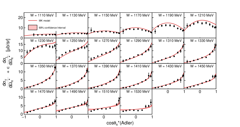
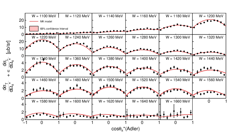
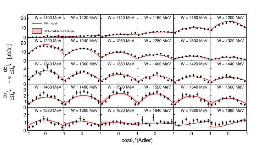
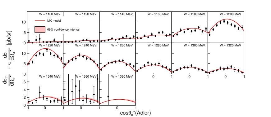
Figures 1, 2, 3 and 4 show some of the fit results for different Q2=0.4superscript𝑄20.4Q^{2}=0.4, 0.52, 0.65, 0.9 GeV, with exclusive electron-induced reactions data within 1σ1𝜎1\sigma error band, where the reduced χ2=2.32superscript𝜒22.32\chi^{2}=2.32.

Refer to caption
Figure 1: Fit results for dσTdΩπ+ϵdσLdΩπ𝑑subscript𝜎𝑇𝑑subscriptsuperscriptΩ𝜋italic-ϵ𝑑subscript𝜎𝐿𝑑subscriptsuperscriptΩ𝜋\frac{d\sigma_{T}}{d\Omega^{\ast}_{\pi}}+\epsilon\frac{d\sigma_{L}}{d\Omega^{\ast}_{\pi}} at Q2=0.4(GeV/c)2superscript𝑄20.4superscriptGeV𝑐2Q^{2}=0.4~{}(\text{GeV}/c)^{2} and Ee=1.515subscript𝐸𝑒1.515E_{e}=1.515 GeV for epenπ+𝑒𝑝𝑒𝑛superscript𝜋ep\rightarrow en\pi^{+} channel from the MK model. Best values are shown as the solid red line with 68%percent6868\% confidence interval.
Refer to caption
Figure 2: Fit results for dσTdΩπ+ϵdσLdΩπ𝑑subscript𝜎𝑇𝑑subscriptsuperscriptΩ𝜋italic-ϵ𝑑subscript𝜎𝐿𝑑subscriptsuperscriptΩ𝜋\frac{d\sigma_{T}}{d\Omega^{\ast}_{\pi}}+\epsilon\frac{d\sigma_{L}}{d\Omega^{\ast}_{\pi}} at Q2=0.52(GeV/c)2superscript𝑄20.52superscriptGeV𝑐2Q^{2}=0.52~{}(\text{GeV}/c)^{2} and Ee=1.645subscript𝐸𝑒1.645E_{e}=1.645 GeV for epepπ0𝑒𝑝𝑒𝑝superscript𝜋0ep\rightarrow ep\pi^{0} channel from the MK model. Best values are shown as the solid red line with 68%percent6868\% confidence interval.
Refer to caption
Figure 3: Fit results for dσTdΩπ+ϵdσLdΩπ𝑑subscript𝜎𝑇𝑑subscriptsuperscriptΩ𝜋italic-ϵ𝑑subscript𝜎𝐿𝑑subscriptsuperscriptΩ𝜋\frac{d\sigma_{T}}{d\Omega^{\ast}_{\pi}}+\epsilon\frac{d\sigma_{L}}{d\Omega^{\ast}_{\pi}} at Q2=0.65(GeV/c)2superscript𝑄20.65superscriptGeV𝑐2Q^{2}=0.65~{}(\text{GeV}/c)^{2} and Ee=2.445subscript𝐸𝑒2.445E_{e}=2.445 GeV for epepπ0𝑒𝑝𝑒𝑝superscript𝜋0ep\rightarrow ep\pi^{0} channel from the MK model. Best values are shown as the solid red line with 68%percent6868\% confidence interval.
Refer to caption
Figure 4: Fit results for dσTdΩπ+ϵdσLdΩπ𝑑subscript𝜎𝑇𝑑subscriptsuperscriptΩ𝜋italic-ϵ𝑑subscript𝜎𝐿𝑑subscriptsuperscriptΩ𝜋\frac{d\sigma_{T}}{d\Omega^{\ast}_{\pi}}+\epsilon\frac{d\sigma_{L}}{d\Omega^{\ast}_{\pi}} at Q2=0.9(GeV/c)2superscript𝑄20.9superscriptGeV𝑐2Q^{2}=0.9~{}(\text{GeV}/c)^{2} and Ee=1.645subscript𝐸𝑒1.645E_{e}=1.645 GeV for epepπ0𝑒𝑝𝑒𝑝superscript𝜋0ep\rightarrow ep\pi^{0} channel from the MK model. Best values are shown as the solid red line with 68%percent6868\% confidence interval.

The fit results show that the best form factors for the resonances with spin-3/2 are:

C3(p)superscriptsubscript𝐶3𝑝\displaystyle C_{3}^{(p)} =\displaystyle= A(1k2/MV2)211k2/DMV2𝐴superscript1superscript𝑘2superscriptsubscript𝑀𝑉2211superscript𝑘2𝐷superscriptsubscript𝑀𝑉2\displaystyle\frac{A}{(1-k^{2}/M_{V}^{2})^{2}}\frac{1}{1-k^{2}/DM_{V}^{2}}
C4(p)superscriptsubscript𝐶4𝑝\displaystyle C_{4}^{(p)} =\displaystyle= B(1k2/MV2)211k2/DMV2𝐵superscript1superscript𝑘2superscriptsubscript𝑀𝑉2211superscript𝑘2𝐷superscriptsubscript𝑀𝑉2\displaystyle\frac{B}{(1-k^{2}/M_{V}^{2})^{2}}\frac{1}{1-k^{2}/DM_{V}^{2}}
C5(p)superscriptsubscript𝐶5𝑝\displaystyle C_{5}^{(p)} =\displaystyle= C(1k2/MV2)2,𝐶superscript1superscript𝑘2superscriptsubscript𝑀𝑉22\displaystyle\frac{C}{(1-k^{2}/M_{V}^{2})^{2}}, (8)

while for resonances with spin-1/2 the following form factors are proposed:

g1(p)superscriptsubscript𝑔1𝑝\displaystyle g_{1}^{(p)} =\displaystyle= A(1k2/MV2)2[1Bln(1k21GeV2)]𝐴superscript1superscript𝑘2superscriptsubscript𝑀𝑉22delimited-[]1𝐵1superscript𝑘21superscriptGeV2\displaystyle\frac{A}{(1-k^{2}/M_{V}^{2})^{2}}\left[1-B\ln\left(1-\frac{k^{2}}{1\text{GeV}^{2}}\right)\right]
g2(p)superscriptsubscript𝑔2𝑝\displaystyle g_{2}^{(p)} =\displaystyle= C(1k2/MV2)2.𝐶superscript1superscript𝑘2superscriptsubscript𝑀𝑉22\displaystyle\frac{C}{(1-k^{2}/M_{V}^{2})^{2}}. (9)

where MV=0.84subscript𝑀𝑉0.84M_{V}=0.84. The best fit form-factor for resonances P33(1600)subscript𝑃331600P_{33}(1600), S31(1620)subscript𝑆311620S_{31}(1620) and F15(1680)subscript𝐹151680F_{15}(1680) are:

FVsubscript𝐹𝑉\displaystyle F_{V} =\displaystyle= A(1k2MV2)2(1k2M2)n/2.𝐴superscript1superscript𝑘2superscriptsubscript𝑀𝑉22superscript1superscript𝑘2superscript𝑀2𝑛2\displaystyle A\left(1-\frac{k^{2}}{M_{V}^{2}}\right)^{-2}\left(1-\frac{k^{2}}{M^{2}}\right)^{n/2}. (10)

In all defined form factors, A B C and D are the free parameters that were fit to the data and their best values are listed in Table 3.

Table 3: Fit result for resonance form factor
Resonance A B C D
P33(1232)subscript𝑃331232P_{33}(1232) -2.028 1.813 -0.17 4.73
P11(1440)subscript𝑃111440P_{11}(1440) 1.685 2.547 0.494
D13(1520)subscript𝐷131520D_{13}(1520) -3.689 3.687 -0.72 1.065
S11(1535)subscript𝑆111535S_{11}(1535) 2.529 1.093 0.449
P33(1600)subscript𝑃331600P_{33}(1600) 0.807
S31(1620)subscript𝑆311620S_{31}(1620) 1.510
F15(1680)subscript𝐹151680F_{15}(1680) 1.155
Refer to caption
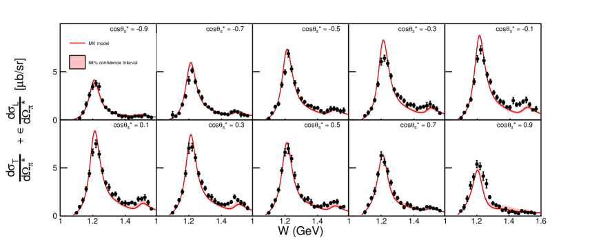
Figure 5: Comparison of the MK model with electron scattering data for different cosθπsubscriptsuperscript𝜃𝜋\cos\theta^{\ast}_{\pi} in the at Q2=1.15(GeV/c)2superscript𝑄21.15superscriptGeV𝑐2Q^{2}=1.15~{}(\text{GeV}/c)^{2} and Ee=2.445subscript𝐸𝑒2.445E_{e}=2.445 GeV for epepπ0𝑒𝑝𝑒𝑝superscript𝜋0ep\rightarrow ep\pi^{0} channel. The predictions of MK model are shown as the solid red lines with 68%percent6868\% confidence interval and the reduced χ2=3.979superscript𝜒23.979\chi^{2}=3.979. Date is from reference [15].

The proposed form factors for the proton in nonresonant interactions are very similar to the one in the original MK model [17]:

F1(p)superscriptsubscript𝐹1𝑝\displaystyle F_{1}^{(p)} =\displaystyle= 11+τ[1+τ1+λnτ(0.59+λnμpτ)]GE11𝜏delimited-[]1𝜏1subscript𝜆𝑛𝜏0.59subscript𝜆𝑛subscript𝜇𝑝𝜏subscript𝐺𝐸\displaystyle\frac{1}{1+\tau}\left[1+\frac{\tau}{1+\lambda_{n}\tau}\left(0.59+\lambda_{n}\mu_{p}\tau\right)\right]G_{E}
μpF2(p)subscript𝜇𝑝superscriptsubscript𝐹2𝑝\displaystyle\mu_{p}F_{2}^{(p)} =\displaystyle= 11+τ[μp1+2.2τ1+λnτ]GE11𝜏delimited-[]subscript𝜇𝑝12.2𝜏1subscript𝜆𝑛𝜏subscript𝐺𝐸\displaystyle\frac{1}{1+\tau}\left[\mu_{p}-1+\frac{2.2\tau}{1+\lambda_{n}\tau}\right]G_{E} (11)

with two adjustable parameters β1subscript𝛽1\beta_{1} and β2subscript𝛽2\beta_{2} in:

GEsubscript𝐺𝐸\displaystyle G_{E} =\displaystyle= (11k2/β1MV2)2superscript11superscript𝑘2subscript𝛽1superscriptsubscript𝑀𝑉22\displaystyle\left(\frac{1}{1-k^{2}/\beta_{1}M_{V}^{2}}\right)^{2}
τ𝜏\displaystyle\tau =\displaystyle= β2k2/4M2subscript𝛽2superscript𝑘24superscript𝑀2\displaystyle-\beta_{2}k^{2}/4M^{2} (12)

where β1=0.896subscript𝛽10.896\beta_{1}=0.896 and β2=2.15subscript𝛽22.15\beta_{2}=2.15333 Fvir(W)=8.09W341.68W2+66.34W32.5733subscript𝐹𝑣𝑖𝑟𝑊8.09superscript𝑊341.68superscript𝑊266.34𝑊32.5733F_{vir}(W)=8.09W^{3}-41.68W^{2}+66.34W-32.5733 (for 1.3 GeVW<1.6 GeV1.3 GeV𝑊1.6 GeV1.3\text{ GeV}\leq W<1.6\text{ GeV}).

IV Results for electron-induced data

Figure 5 shows the MK model predictions for different pion angles and hadronic invariant mass at Q2=1.15(GeV/c)2superscript𝑄21.15superscriptGeV𝑐2Q^{2}=1.15~{}(\text{GeV}/c)^{2} where it is outside the kinematic region of the fitted data in our analysis (Q2<0.9(GeV/c)2superscript𝑄20.9superscriptGeV𝑐2Q^{2}<0.9~{}(\text{GeV}/c)^{2}). The data shows the single π0superscript𝜋0\pi^{0} production measurement for the different pion polar angles (in the hadronic rest frame) in terms of the invariant mass.

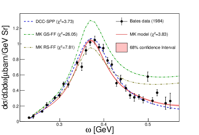
The MK model prediction can also be compared with inclusive electron scattering data. However it is important to note that the MK model can only predict a single pion in the final state while the data is the measurements of one or more pions in the final state. Therefore they are not identical, however at low (ω𝜔\omega, W𝑊W) only a single pion can be produced in the final states, for example when Ee<1subscript𝐸𝑒1E_{e}<1 GeV or when W<1.4𝑊1.4W<1.4 GeV.

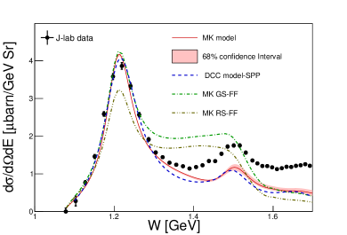
Figure 6 shows the inclusive electron-proton differential cross section in terms of energy transferred (ω𝜔\omega) at Ee=0.73subscript𝐸𝑒0.73E_{e}=0.73 GeV, where exact agreement with data is expected. On the other hand, Fig. 7 shows the same measurement at higher energy (Ee=3.04subscript𝐸𝑒3.04E_{e}=3.04 GeV) where good agreements is expected in the ΔΔ\Delta region. To show the MK model improvements, the predictions of original MK model with the RS and the GS form-factors are displayed. The DCC model prediction for SPP are also presented. In Figure 6 where the data and the models are identical, the reduced χ2superscript𝜒2\chi^{2} are added to the legend which shows the MK and the DCC models have similar agreements with data. This also indicates that the MK model is significantly improved as χ2superscript𝜒2\chi^{2} is reduced from 26.05 to 3.83.

Refer to caption
Figure 6: Inclusive differential cross section data in terms of energy transferred in the lab frame from reference [18] at Ee=0.73subscript𝐸𝑒0.73E_{e}=0.73 GeV and θe=37.1subscript𝜃𝑒superscript37.1\theta_{e}=37.1^{\circ} (Q20.11(GeV/c)2similar-tosuperscript𝑄20.11superscriptGeV𝑐2Q^{2}\sim 0.11(\text{GeV}/c)^{2}). Updated MK model shown as the solid red lines with 68%percent6868\%confidence interval while the original MK model with GS form-factors (GS-FF) and RS form-factors (RS-FF) are shown in dashed-dotted lines. DCC model [13] prediction for SPP is showed with dashed blue line.
Refer to caption
Figure 7: Inclusive differential cross section data from [19] at Ee=3.04subscript𝐸𝑒3.04E_{e}=3.04 GeV and θe=12subscript𝜃𝑒superscript12\theta_{e}=12^{\circ} (Q20.170.36(GeV/c)2similar-tosuperscript𝑄20.170.36superscriptGeV𝑐2Q^{2}\sim 0.17-0.36(\text{GeV}/c)^{2}). Updated MK model shown as the red lines with 68%percent6868\% confidence interval while the original MK model with GS form-factors (GS-FF) and RS form-factors (RS-FF) are shown in dashed-dotted lines. DCC model [13] prediction for SPP is showed with dashed blue line.

V conclusion

In this work the vector current form-factors of the MK model were improved by introducing new helicity amplitudes for resonances in the first and the second resonance regions. The free parameters of the model are fit to exclusive electron scattering data to constrain the vector form factors of resonances (up to W=1.68𝑊1.68W=1.68 GeV) and the proton in the nonresonant interaction and evaluated the total uncertainty on cross-sections prediction.

The goodness-of-fit of the model to the data shows that the pre-fit model covers the data. Further validation of the constrained model against inclusive electron scattering data sets demonstrates the robustness of the constrained model and its predictive power.

Acknowledgements.
I would like to express my special thanks to Philip Rodrigues who provided insight and expertise that greatly assisted the research. I would also like to thank Satoshi Nakamura, Lukas Koch and Daniel Cherdack for their comments that greatly improved the results and manuscript.
I am extremely grateful to Dave Wark, Kevin Mc Farland, and FNAL for being a constant source of encouragement and support.

Appendix A

The V-A helicity amplitudes of MK model is defined in reference [1], however the helicity amplitudes of vector current are given in Table 4 for convenience.

Table 4: Vector helicity amplitudes of resonant interaction.
λ2subscript𝜆2\lambda_{2} λ1subscript𝜆1\lambda_{1} F~λ2λ1eL(θ,ϕ)superscriptsubscript~𝐹subscript𝜆2subscript𝜆1subscript𝑒𝐿𝜃italic-ϕ\tilde{F}_{\lambda_{2}\lambda_{1}}^{e_{L}}(\theta,\phi) F~λ2λ1eR(θ,ϕ)superscriptsubscript~𝐹subscript𝜆2subscript𝜆1subscript𝑒𝑅𝜃italic-ϕ\tilde{F}_{\lambda_{2}\lambda_{1}}^{e_{R}}(\theta,\phi)
12121212
missing-subexpression
missing-subexpression1212missing-subexpression1212
\begin{aligned} &\scalebox{0.001}{~{}}\\ &\frac{1}{2}\\[7.0pt] -&\frac{1}{2}\\[7.0pt] &\frac{1}{2}\\[7.0pt] -&\frac{1}{2}\end{aligned}
12121212
missing-subexpression
missing-subexpression12missing-subexpression121212
\begin{aligned} &\scalebox{0.001}{~{}}\\ &\frac{1}{2}\\[7.0pt] &\frac{1}{2}\\[7.0pt] -&\frac{1}{2}\\[7.0pt] -&\frac{1}{2}\end{aligned}
±j2j+12𝒟j(R)f3V(R(I,j=l±12))d3212j(θ)e2iϕj2j+12𝒟j(R)f3V(R(I,j=l±12))d3212j(θ)eiϕj2j+12𝒟j(R)f1V(R(I,j=l±12))d1212j(θ)eiϕj2j+12𝒟j(R)f1V(R(I,j=l±12))d1212j(θ)
missing-subexpression
plus-or-minussubscript𝑗2𝑗12superscript𝒟𝑗𝑅subscriptsuperscript𝑓𝑉3𝑅𝐼𝑗plus-or-minus𝑙12subscriptsuperscript𝑑𝑗3212𝜃superscript𝑒2𝑖italic-ϕmissing-subexpressionsubscript𝑗2𝑗12superscript𝒟𝑗𝑅subscriptsuperscript𝑓𝑉3𝑅𝐼𝑗plus-or-minus𝑙12subscriptsuperscript𝑑𝑗3212𝜃superscript𝑒𝑖italic-ϕminus-or-plussubscript𝑗2𝑗12superscript𝒟𝑗𝑅subscriptsuperscript𝑓𝑉1𝑅𝐼𝑗plus-or-minus𝑙12subscriptsuperscript𝑑𝑗1212𝜃superscript𝑒𝑖italic-ϕsubscript𝑗2𝑗12superscript𝒟𝑗𝑅subscriptsuperscript𝑓𝑉1𝑅𝐼𝑗plus-or-minus𝑙12subscriptsuperscript𝑑𝑗1212𝜃
\begin{aligned} &\scalebox{0.001}{~{}}\\ \pm&\sum_{j}\frac{2j+1}{\sqrt{2}}\mathcal{D}^{j}(R)~{}f^{V}_{-3}(R(I,j=l\pm\frac{1}{2}))~{}d^{j}_{\frac{3}{2}\frac{1}{2}}(\theta)e^{-2i\phi}\\ &\sum_{j}\frac{2j+1}{\sqrt{2}}\mathcal{D}^{j}(R)~{}f^{V}_{-3}(R(I,j=l\pm\frac{1}{2}))~{}d^{j}_{\frac{3}{2}-\frac{1}{2}}(\theta)e^{-i\phi}\\ \mp&\sum_{j}\frac{2j+1}{\sqrt{2}}\mathcal{D}^{j}(R)~{}f^{V}_{-1}(R(I,j=l\pm\frac{1}{2}))~{}d^{j}_{\frac{1}{2}\frac{1}{2}}(\theta)e^{-i\phi}\\ -&\sum_{j}\frac{2j+1}{\sqrt{2}}\mathcal{D}^{j}(R)~{}f^{V}_{-1}(R(I,j=l\pm\frac{1}{2}))~{}d^{j}_{\frac{1}{2}-\frac{1}{2}}(\theta)\\ \end{aligned}
j2j+12𝒟j(R)f1V(R(I,j=l±12))d1212j(θ)±j2j+12𝒟j(R)f1V(R(I,j=l±12))d1212j(θ)eiϕj2j+12𝒟j(R)f3V(R(I,j=l±12))d3212j(θ)eiϕ±j2j+12𝒟j(R)f3V(R(I,j=l±12))d3212j(θ)e2iϕ
missing-subexpression
subscript𝑗2𝑗12superscript𝒟𝑗𝑅subscriptsuperscript𝑓𝑉1𝑅𝐼𝑗plus-or-minus𝑙12subscriptsuperscript𝑑𝑗1212𝜃plus-or-minussubscript𝑗2𝑗12superscript𝒟𝑗𝑅subscriptsuperscript𝑓𝑉1𝑅𝐼𝑗plus-or-minus𝑙12subscriptsuperscript𝑑𝑗1212𝜃superscript𝑒𝑖italic-ϕsubscript𝑗2𝑗12superscript𝒟𝑗𝑅subscriptsuperscript𝑓𝑉3𝑅𝐼𝑗plus-or-minus𝑙12subscriptsuperscript𝑑𝑗3212𝜃superscript𝑒𝑖italic-ϕplus-or-minussubscript𝑗2𝑗12superscript𝒟𝑗𝑅subscriptsuperscript𝑓𝑉3𝑅𝐼𝑗plus-or-minus𝑙12subscriptsuperscript𝑑𝑗3212𝜃superscript𝑒2𝑖italic-ϕ
\begin{aligned} &\scalebox{0.01}{~{}}\\ -&\sum_{j}\frac{2j+1}{\sqrt{2}}\mathcal{D}^{j}(R)~{}f^{V}_{-1}(R(I,j=l\pm\frac{1}{2}))~{}d^{j}_{\frac{1}{2}-\frac{1}{2}}(\theta)\\ \pm&\sum_{j}\frac{2j+1}{\sqrt{2}}\mathcal{D}^{j}(R)~{}f^{V}_{-1}(R(I,j=l\pm\frac{1}{2}))~{}d^{j}_{\frac{1}{2}\frac{1}{2}}(\theta)e^{i\phi}\\ -&\sum_{j}\frac{2j+1}{\sqrt{2}}\mathcal{D}^{j}(R)~{}f^{V}_{-3}(R(I,j=l\pm\frac{1}{2}))~{}d^{j}_{\frac{3}{2}-\frac{1}{2}}(\theta)e^{i\phi}\\ \pm&\sum_{j}\frac{2j+1}{\sqrt{2}}\mathcal{D}^{j}(R)~{}f^{V}_{-3}(R(I,j=l\pm\frac{1}{2}))~{}d^{j}_{\frac{3}{2}\frac{1}{2}}(\theta)e^{2i\phi}\end{aligned}
F~λ2λ1e(θ,ϕ)superscriptsubscript~𝐹subscript𝜆2subscript𝜆1subscript𝑒𝜃italic-ϕ\tilde{F}_{\lambda_{2}\lambda_{1}}^{e_{-}}(\theta,\phi) F~λ2λ1e+(θ,ϕ)superscriptsubscript~𝐹subscript𝜆2subscript𝜆1subscript𝑒𝜃italic-ϕ\tilde{F}_{\lambda_{2}\lambda_{1}}^{e_{+}}(\theta,\phi)
12121212
missing-subexpression
missing-subexpression1212missing-subexpression1212
\begin{aligned} &\scalebox{0.001}{~{}}\\ &\frac{1}{2}\\[7.0pt] -&\frac{1}{2}\\[7.0pt] &\frac{1}{2}\\[7.0pt] -&\frac{1}{2}\end{aligned}
12121212
missing-subexpression
missing-subexpression12missing-subexpression121212
\begin{aligned} &\scalebox{0.001}{~{}}\\ &\frac{1}{2}\\[7.0pt] &\frac{1}{2}\\[7.0pt] -&\frac{1}{2}\\[7.0pt] -&\frac{1}{2}\end{aligned}
|𝐤|k2j2j+12𝒟j(R)f0+V()(R(I,j=l±12))d1212j(θ)eiϕ±|𝐤|k2j2j+12𝒟j(R)f0+V()(R(I,j=l±12))d1212j(θ)±|𝐤|k2j2j+12𝒟j(R)f0+V()(R(I,j=l±12))d1212j(θ)|𝐤|k2j2j+12𝒟j(R)f0+V()(R(I,j=l±12))d1212j(θ)eiϕ
missing-subexpression
missing-subexpression𝐤superscript𝑘2subscript𝑗2𝑗12superscript𝒟𝑗𝑅subscriptsuperscript𝑓𝑉limit-from0𝑅𝐼𝑗plus-or-minus𝑙12subscriptsuperscript𝑑𝑗1212𝜃superscript𝑒𝑖italic-ϕplus-or-minus𝐤superscript𝑘2subscript𝑗2𝑗12superscript𝒟𝑗𝑅subscriptsuperscript𝑓𝑉limit-from0𝑅𝐼𝑗plus-or-minus𝑙12subscriptsuperscript𝑑𝑗1212𝜃plus-or-minus𝐤superscript𝑘2subscript𝑗2𝑗12superscript𝒟𝑗𝑅subscriptsuperscript𝑓𝑉limit-from0𝑅𝐼𝑗plus-or-minus𝑙12subscriptsuperscript𝑑𝑗1212𝜃𝐤superscript𝑘2subscript𝑗2𝑗12superscript𝒟𝑗𝑅subscriptsuperscript𝑓𝑉limit-from0𝑅𝐼𝑗plus-or-minus𝑙12subscriptsuperscript𝑑𝑗1212𝜃superscript𝑒𝑖italic-ϕ
\begin{aligned} &\scalebox{0.05}{~{}}\\ &\frac{|\mathbf{k}|}{\sqrt{-k^{2}}}\sum_{j}\frac{2j+1}{\sqrt{2}}\mathcal{D}^{j}(R)~{}f^{V(-)}_{0+}(R(I,j=l\pm\frac{1}{2}))~{}d^{j}_{\frac{1}{2}\frac{1}{2}}(\theta)e^{-i\phi}\\ \pm&\frac{|\mathbf{k}|}{\sqrt{-k^{2}}}\sum_{j}\frac{2j+1}{\sqrt{2}}\mathcal{D}^{j}(R)~{}f^{V(-)}_{0+}(R(I,j=l\pm\frac{1}{2}))~{}d^{j}_{\frac{1}{2}-\frac{1}{2}}(\theta)\\ \pm&\frac{|\mathbf{k}|}{\sqrt{-k^{2}}}\sum_{j}\frac{2j+1}{\sqrt{2}}\mathcal{D}^{j}(R)~{}f^{V(-)}_{0+}(R(I,j=l\pm\frac{1}{2}))~{}d^{j}_{\frac{1}{2}-\frac{1}{2}}(\theta)\\ -&\frac{|\mathbf{k}|}{\sqrt{-k^{2}}}\sum_{j}\frac{2j+1}{\sqrt{2}}\mathcal{D}^{j}(R)~{}f^{V(-)}_{0+}(R(I,j=l\pm\frac{1}{2}))~{}d^{j}_{\frac{1}{2}\frac{1}{2}}(\theta)e^{i\phi}\end{aligned}
|𝐤|k2j2j+12𝒟j(R)f0+V(+)(R(I,j=l±12))d1212j(θ)eiϕ±|𝐤|k2j2j+12𝒟j(R)f0+V(+)(R(I,j=l±12))d1212j(θ)±|𝐤|k2j2j+12𝒟j(R)f0+V(+)(R(I,j=l±12))d1212j(θ)|𝐤|k2j2j+12𝒟j(R)f0+V(+)(R(I,j=l±12))d1212j(θ)eiϕ
missing-subexpression
missing-subexpression𝐤superscript𝑘2subscript𝑗2𝑗12superscript𝒟𝑗𝑅subscriptsuperscript𝑓𝑉limit-from0𝑅𝐼𝑗plus-or-minus𝑙12subscriptsuperscript𝑑𝑗1212𝜃superscript𝑒𝑖italic-ϕplus-or-minus𝐤superscript𝑘2subscript𝑗2𝑗12superscript𝒟𝑗𝑅subscriptsuperscript𝑓𝑉limit-from0𝑅𝐼𝑗plus-or-minus𝑙12subscriptsuperscript𝑑𝑗1212𝜃plus-or-minus𝐤superscript𝑘2subscript𝑗2𝑗12superscript𝒟𝑗𝑅subscriptsuperscript𝑓𝑉limit-from0𝑅𝐼𝑗plus-or-minus𝑙12subscriptsuperscript𝑑𝑗1212𝜃𝐤superscript𝑘2subscript𝑗2𝑗12superscript𝒟𝑗𝑅subscriptsuperscript𝑓𝑉limit-from0𝑅𝐼𝑗plus-or-minus𝑙12subscriptsuperscript𝑑𝑗1212𝜃superscript𝑒𝑖italic-ϕ
\begin{aligned} &\scalebox{0.05}{~{}}\\ &\frac{|\mathbf{k}|}{\sqrt{-k^{2}}}\sum_{j}\frac{2j+1}{\sqrt{2}}\mathcal{D}^{j}(R)~{}f^{V(+)}_{0+}(R(I,j=l\pm\frac{1}{2}))~{}d^{j}_{\frac{1}{2}\frac{1}{2}}(\theta)e^{-i\phi}\\ \pm&\frac{|\mathbf{k}|}{\sqrt{-k^{2}}}\sum_{j}\frac{2j+1}{\sqrt{2}}\mathcal{D}^{j}(R)~{}f^{V(+)}_{0+}(R(I,j=l\pm\frac{1}{2}))~{}d^{j}_{\frac{1}{2}-\frac{1}{2}}(\theta)\\ \pm&\frac{|\mathbf{k}|}{\sqrt{-k^{2}}}\sum_{j}\frac{2j+1}{\sqrt{2}}\mathcal{D}^{j}(R)~{}f^{V(+)}_{0+}(R(I,j=l\pm\frac{1}{2}))~{}d^{j}_{\frac{1}{2}-\frac{1}{2}}(\theta)\\ -&\frac{|\mathbf{k}|}{\sqrt{-k^{2}}}\sum_{j}\frac{2j+1}{\sqrt{2}}\mathcal{D}^{j}(R)~{}f^{V(+)}_{0+}(R(I,j=l\pm\frac{1}{2}))~{}d^{j}_{\frac{1}{2}\frac{1}{2}}(\theta)e^{i\phi}\end{aligned}

References

  • Kabirnezhad [2018] M. Kabirnezhad, Phys. Rev. D 97, 013002 (2018).
  • Rein and Sehgal [1981] D. Rein and L. M. Sehgal, Annals Phys. 133, 79 (1981).
  • Rein [1987] D. Rein, Z. Phys. C 35, 43 (1987).
  • Adler [1968] S. L. Adler, Annals Phys. 50, 189 (1968).
  • Hernandez et al. [2007] E. Hernandez, J. Nieves, and M. Valverde, Phys. Rev. D 76, 033005 (2007).
  • Sato et al. [2003] T. Sato, D. Uno, and T. S. H. Lee, Phys. Rev. C 67, 065201 (2003).
  • Yao et al. [2019] D.-L. Yao, L. Alvarez-Ruso, and M. Vicente Vacas, Phys. Lett. B 794, 109 (2019)arXiv:1901.00773 [hep-ph] .
  • Gonz lez-Jim nez et al. [2019] R. Gonz lez-Jim nez, A. Nikolakopoulos, N. Jachowicz, and J. Ud as, Phys. Rev. C 100, 045501 (2019).
  • Amaro et al. [2019] J. Amaro, M. Barbaro, J. Caballero, R. Gonz lez-Jim nez, G. Megias, and I. Ruiz Simo,   (2019), arXiv:1912.10612 [nucl-th] .
  • Hayato [2009] Y. Hayato, Acta Phys. Polon. B 40, 2477 (2009).
  • Andreopoulos and et al. [2010] C. Andreopoulos and et al., Nucl. Instrum. Meth. A 614, 87 (2010).
  • Lalakulich et al. [2006] O. Lalakulich, E. A. Paschos, and G. Piranishvili, Phys. Rev. D 74, 014009 (2006).
  • Nakamura et al. [2015] S. X. Nakamura, H. Kamano, and T. Sato, Phys. Rev. D 92, 074024 (2015).
  • Graczyk and Sobczyk [2008] K. M. Graczyk and J. T. Sobczyk, Phys. Rev. D 77, 053001 (2008).
  • Joo and et al. [CLAS Collaboration] [2002] K. Joo and et al. [CLAS Collaboration], Phys. Rev. lett. 88, 122001 (2002).
  • Egiyan and et al. [CLAS Collaboration] [2006] H. Egiyan and et al. [CLAS Collaboration], Phys. Rev. C 73, 025204 (2006).
  • Galster et al. [1971] S. Galster, H. Klein, J. Moritz, K. H. Schmidt, D. Wegener, and J. Bleckwenn, Nucl. Phys. B 32, 221 (1971).
  • O’Connell et al. [1984] J. O’Connell et al., Phys. Rev. Lett. 53, 1627 (1984).
  • [19]  Preliminary results from JLab E00-002, C. Keppel and M. I. Niculescu, spokespersons. Data files can be obtained at https://hallcweb.jlab.org/resdata/database.