The Power of Connection:
Leveraging Network Analysis
to Advance Receivable Financing

Abstract

Receivable financing is the process whereby cash is advanced to firms against receivables their customers have yet to pay: a receivable can be sold to a funder, which immediately gives the firm cash in return for a small percentage of the receivable amount as a fee. Receivable financing has been traditionally handled in a centralized way, where every request is processed by the funder individually and independently of one another.

In this work we propose a novel, network-based approach to receivable financing, which enables customers of the same funder to autonomously pay each other as much as possible, and gives benefits to both the funder (reduced cash anticipation and exposure risk) and its customers (smaller fees and lightweight service establishment).

Our main contributions consist in providing a principled formulation of the network-based receivable-settlement strategy, and showing how to achieve all algorithmic challenges posed by the design of this strategy. We formulate network-based receivable financing as a novel combinatorial-optimization problem on a multigraph of receivables. We show that the problem is $\mathbf{NP}$-hard, and devise an exact branch-and-bound algorithm, as well as algorithms to efficiently find effective approximate solutions. Our more efficient algorithms are based on cycle enumeration and selection, and exploit a theoretical characterization in terms of a knapsack problem, as well as a refining strategy that properly adds paths between cycles. We also investigate the real-world issue of avoiding temporary violations of the problem constraints, and design methods for handling it.

An extensive experimental evaluation is performed on real receivable data. Results attest the good performance of our methods.

1 Introduction

The term receivable indicates a debt owed to a creditor, which the debtor has not yet paid for.

Receivable Financing (RF) is a service for creditors to fund cash flow by selling accounts receivables to a funder or financing company. The funder anticipates (a proportion of) the receivable amount to the creditor, deducting a percentage as a fee for the service.

Receivable financing mainly exists to shorten the waiting times of receivable payment. These typically range from 30 to 120 days, which means that businesses face a nervous wait as they cannot effectively plan ahead without knowing when their next payment is coming in. Cashing anticipated payment for a receivable gives a business instant access to a lump sum of capital, which significantly eases the cash-flow issues associated with receivables. Another pro is that funders typically manage credit control too, meaning that credit control is outsourced and creditors no longer need to chase up debtors for receivable payment.

RF has traditionally been provided by banks and financial institutions. Recently, digital platforms have emerged as well, e.g., BlueVine, Fundbox, C2FO, MarketInvoice. Nevertheless, while digital funders are rapidly growing, they are still far from saturating the commercial credit market.

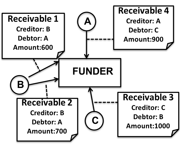
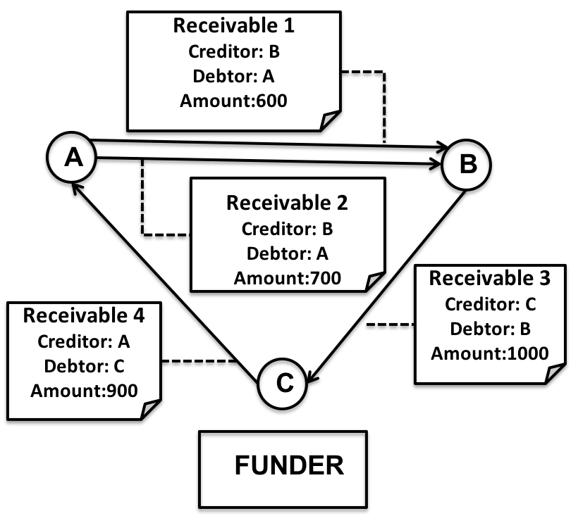
Figure 1: Client/server (left) vs. network-based (right) receivable financing. In the first case, the funder handles each request individually, paying a total amount of 3200. In the network-based scenario, customers are allowed to pay each other. Assume $A$, $B$, $C$ have $0$, $1000$, $0$ on their accounts, respectively. Then, $B$ has sufficient money to pay Receivable 3, which in turns makes $C$ have enough money to pay Receivable 4, and so on, until all receivables have been paid. This way no money is anticipated by the funder.

A novel, network-based perspective. Existing RF services employ an inherently client-server perspective: the funder, just like a centralized server, receives multiple funding requests, and processes each of them individually.

It is easy to observe that this strategy has an obvious limitation, i.e., it overlooks the fact that a set of receivables for which the RF service is simultaneously requested compose a network where a customer may act as the creditor or the debtor of different receivables. In this work we present a novel receivable-financing method, which leverages such a network perspective to enable an autonomous cash flow among customers. For instance, as shown in Figure 1, a network-based RF service might allow the funder to anticipate no money, while still having RF accomplished for all the receivables. A real scenario is clearly more complicated than the simple one depicted in the example. This means that the receivables that can be autonomously paid by the customers without involving the funder are typically only a subset of all the receivable which the RF service is requested for. The main goal in the design of network-based RF is therefore to select the largest-amount subset of receivables for which autonomous payment is possible.

Network-based RF provides noticeable advantages to both the funder and the customers. In fact, the funder can now entrust to the novel network-based settlement system the settlement of the receivable financing requests advanced by the customers who accept to enroll into it. The system takes care to enable autonomous payment of these receivables to the maximum extent possible. This means that the funder no longer needs to anticipate cash for each request, achieving a larger availability of liquidity, and a lower risk of incurring into payment delays or credit losses. The increased cash availability in turn allows the funder to devise proper marketing strategies to attract more customers to try the novel settlement service. Specifically, the funder offers the customers the benefit of a lower fee on each incoming deliverable. A further advantage for the customer is the easier access to the receivable financing service (in terms of both time and effort), which is enabled by the employment of lighter bureaucracy and risk-assessment rules.

A crucial aspect for the network-based RF service to work properly is to regulate it with to a do-ut-des mechanism, where customers accept to pay selected receivables, for which they act as a debtor, possibly earlier than they would do without the service. Our enrolling customer is warned that the system does not allow non-payments, and that when a receivable for which she plays as debtor is selected for settlement, its amount is automatically transferred to the creditor. However, the customer is informed that she also benefits from early payments, because the system ensures that they increase the chance for a debtor of subsequently acting as a creditor. Moreover, customers may preserve their freedom on how to handle payments, by choosing which requests to submit to the network-based system.

Challenges and contributions. In this work we tackle a real-world problem from a specific application domain, i.e., receivable financing, proposing a novel method, based on a network-perspective that – to the best of our knowledge – has never been employed for such a problem before. Effectively solving the network-based receivable-settlement problem requires non-trivial algorithmic and theoretic work. This paper focuses on the algorithmic challenges that arise amid the design of a such a network-based approach.

We observe that the set of receivables that are available for settlement at any day can be naturally modeled as a multigraph, whose nodes correspond to customers, and an arc from $u$ to $v$ represents a receivable having $u$ as a debtor and $v$ as a creditor. Such a multigraph is arc-weighted, with weights corresponding to receivable amounts, and node-attributed, as every node is assigned its account balance(s), as well as a floor and a cap, which serve the purpose of limiting the balance(s) of a node to stay within a reasonable range. We formulate network-based receivable settlement as a novel combinatorial-optimization problem on a multigraph of receivables, whose objective is to select a subset of arcs so as to maximize the total amount of the selected arcs, while also satisfying two constraints: ($i$) the balance of every node meets the corresponding floor-cap constraints, and ($ii$) every node within the output solution is the creditor of at least one output receivable and the debtor of at least one output receivable. We show that the problem is $\mathbf{NP}$-hard and devise both an exact algorithm and effective algorithms to find approximate solutions more efficiently. Our more efficient algorithms exploit the fact that a cycle of the input multigraph is guaranteed to satisfy one of the two problem constraints. For this reason, we formulate a further combinatorial-optimization problem, which identifies a subset of the cycles of the input multigraph, so as to maximize the total amount and keep the floor-cap constraints satisfied. Such a problem is shown to be $\mathbf{NP}$-hard too, and our most efficient algorithms find approximate solutions to it by exploiting a knapsack-like characterization, as well as a refining strategy that properly adds paths between the selected cycles. Orthogonally, we focus on a practical issue that may arise while implementing a network-based RF service in real-world systems: to minimize system re-engineering, it might be required for the money transfers underlying the settled receivables to be executed one at a time and without violating the problem constraints, not even temporarily. We devise proper strategies to handle such a real-world issue, by either redefining floor constraints, or taking a subset of the settled receivables and properly ordering them.

To summarize, the main contributions of this work are:

• We devise a novel, network-based approach to receivable financing (Section 2).

• We provide a principled formulation of the network-based receivable settlement strategy in terms of a novel optimization problem, i.e., Max-profit Balanced Settlement, while also showing the $\mathbf{NP}$-hardness of the problem (Section 3).

• We derive theoretical conditions to bound the objective-function value of a set of problem solutions, and employ them to design an exact branch-and-bound algorithm (Section 4.1).

• We define a further optimization problem, i.e., optimal selection of a subset of cycles, and characterize it in terms of $\mathbf{NP}$-hardness and as a Knapsack problem. Based on such an optimal-cycle-selection problem, we devise an efficient algorithm for the original Max-profit Balanced Settlement problem (Section 4.2).

• We also present a method to improve upon the cycle-selection-based algorithm by suitably adding paths between the selected cycles (Section 4.3). This algorithm and the branch-and-bound one are also combined into a further hybrid algorithm (Section 4.4).

• We handle the real-world scenario where temporary constraint violations are not allowed (Section 4.5).

• We present an extensive evaluation on a real dataset of receivables. Results demonstrate the effectiveness of the proposed methods in practice (Section 6).

In Section 5 we report implementation details, while Section 7 offers related work, and Section 8 draws conclusions.

This is a complete technical report that includes contents from [4] and [5].

2 Preliminaries

In this work we consider the following scenario. We focus on the customer basis $\mathcal{U}$ of a single funder (we assume the funder has no visibility on the customers of other funders). Customers in $\mathcal{U}$ submit RF requests to the funder. We denote by $\mathcal{R}$ the set of receivables submitted to the funder by its customers. The goal of the funder is to select a subset of $\mathcal{R}$ to be settled, by employing a network-based strategy, i.e., making the involved customers pay each other autonomously.

Receivables. Attributes of a receivable $R\in\mathcal{R}$ include:

• $amount(R)\in\mathds{R}$: amount of the receivable;

• $creditor(R)\in\mathcal{U}$: payee of the receivable;

• $debtor(R)\in\mathcal{U}$: payer of the receivable;

• $indate(R)$: date the receivable entered the system;

• $duedate(R)$: date on which the payment falls due;

• $life(R)\in\mathbb{N}$: the maximum number of days the network-based RF service is allowed to try to settle the receivable.

A receivable $R$ is said active for $creditor(R)$, and passive for $debtor(R)$.

Customers. Customers. Customers are assigned a dedicated account by the funder, which is used to pay passive receivables or get paid for active receivables. Moreover, customers may perform deposits/withdrawals on/from their account. Such operations trigger external money flows, which do not derive from receivable settlement. The desideratum to keep the system in a collaborative equilibrium is that, if a customer withdraws money from her account, this operation should not increase the customer’s marginal availability to cash in more receivables through the RF service. Conversely, if a customer deposits money on her account, this operation should obviously increase her ability to pay more receivables. To take into account these principles, we keep track of two different balances in the account of customer $u$, and require such balances to be limited by a floor and a cap (which are set on a customer basis during sign up). As a result, every customer $u\in\mathcal{U}$ is assigned the attributes:

• $bl_{r}(u)\in\mathds{R}$: receivable balance of $u$’s account, i.e., the sum of all receivables $u$ has got paid minus the sum of all receivables $u$ has paid through the RF service over the whole $u$’s lifetime;

• $bl_{a}(u)\in\mathds{R}$: actual balance of $u$’s account, corresponding to the receivable balance $bl_{r}(u)$, increased by money from deposit operations and decreased by withdrawals;

• $cap(u)\in\mathds{R}$: upper bound on the receivable balance of $u$’s account; requiring $bl_{r}(u)\leq cap(u)$ at any time avoids unbalanced situations where a customer utilizes the service only to get money without paying passive receivables;

• $fl(u)\in\mathds{R}$: lower bound on the actual balance of $u$’s account; typically, $fl(u)=0$, but in some cases negative values are allowed, meaning that some overdraft is tolerated.

TABLE I: List of frequent symbols.

symbol	definition
$\mathcal{G}\!=\!(\mathcal{V},\!\mathcal{E},\!w)$	input R-multigraph
$bl_{r}(u)$	receivable balance of $u$’s account ($u\in\mathcal{V}$)
$bl_{a}(u)$	actual balance of $u$’s account ($u\in\mathcal{V}$)
$cap(u)$	upper bound on $bl_{r}(u)$ ($u\in\mathcal{V}$)
$fl(u)$	lower bound on $bl_{a}(u)$ ($u\in\mathcal{V}$)
$\mathscr{C}$	set of cycles in $\mathcal{G}$
$C\in\mathscr{C}$	a cycle in $\mathscr{C}$
$\mathscr{P}_{ij}$	paths from a node in cycle $C_{i}$ to a node in cycle $C_{j}$
$\mathscr{P}_{max}$	max size of a path set in $\{\mathscr{P}_{ij}\}_{i,j}$
$L$;  $L_{p}$	max length of a cycle in $\mathscr{C}$;  max length of a path in $\mathscr{P}_{ij}$
$K;$ $K_{p}$	size of $\mathscr{C}$’s subset;  size of $\mathscr{P}_{ij}$’s subset (beam-search algorithms)
$\mathbf{CC}$	weakly connected components of $\mathcal{G}$
$H$	max size of a $\mathcal{G}$’s conn. component to run the exact algorithm on

Network-based RF in action. The execution flow of our service is as follows. A receivable $R$ is submitted by $creditor(R)$ to the netwok-based RF service. While submitting $R$, the creditor also sets $life(R)$, i.e., the maximum number of days $R$ can stay in the system: if $R$ has not been settled during that period, the creditor gets it back (and she may require to sell it to different financing services).

Once $R$ has been added to the system, $debtor(R)$ is asked to confirm if she agrees with paying $R$ anytime between $indate(R)$ and $duedate(R)$. If $debtor(R)$ gives her confirmation, it means that she accepts to pay $R$ possibly before its $duedate$. This is a crucial aspect in the design of network-based RF. In this regard, a specific mechanism is employed to maintain the desired equilibrium where customers autonomously pay each other as far as possible: the debtor must accept to pay a receivable before its $duedate$ to gain operability within the service, so as to get her (future) active receivables settled more easily. Indeed, according to the constraint $bl_{r}(u)\leq cap(u)$, the more the receivables paid by $u$ through the network-based RF service, the further $bl_{r}(u)$ remains from $cap(u)$ and the higher the chance for $u$ to have her active receivables paid.

After confirmation by $debtor(R)$, $R$ becomes part of the set $\mathcal{R}$ of receivables that the system will attempt to settle (according to the method(s) presented in Sections 3-4). If the system is not able to settle $R$ during the period $[indate(R),\min\{indate(R)+life(R),duedate(R)\}]$, $creditor(R)$ gets the receivable back. Otherwise, $amount(R)$ is withdrawn from the $debtor(R)$’s account and put to the $creditor(R)$’s account. Without loss of generality, we assume that the settlement fee of receivable $R$ is paid by $creditor(R)$ to the funder of the RF service through a different channel. As better explained in Section 3, a receivable $R$ can be selected for settlement only if it complies with the economic conditions of $debtor(R)$’s (and $creditor(R)$’s) account (and some other global constraints are satisfied, see Problem 1). This prevents the system from being affected by insolvencies.

​​​​​​​​​​	​​​​​​
​​​​​​​​​​(a) Day 1	​​​​​​(b) Day 2

Figure 2: An instance of Max-profit Balanced Settlement (Problem 1). Nodes are assigned balances (in this example $bl_{r}$ = $bl_{a}$), and $floor$-$cap$ ranges (square brackets). Arcs are labeled with the amount of the corresponding receivables. Day 1: the arcs depicted with full lines form the optimal solution. No other arcs can be selected. In fact, adding $(\mathrm{E},\mathrm{C})$ and $(\mathrm{C},\mathrm{B})$ to the solution would violate $\mathrm{C}$’s and $\mathrm{E}$’s $floor$ constraint, while adding $(\mathrm{D},\mathrm{A})$ would violate $\mathrm{D}$’s $floor$ constraint. Day 2: receivables present in the system corresponds to the ones not settled at Day 1, along with the two new ones depicted with dotted lines (i.e., $(\mathrm{A},\mathrm{E})$ and $(\mathrm{C},\mathrm{A})$). The optimal solution at Day 2 is an empty set. In fact, the only way to have Problem  1’s Constraint (2) satisfied would be selecting $(\mathrm{A},\mathrm{E})$, $(\mathrm{E},\mathrm{C})$, and $(\mathrm{C},\mathrm{A})$ altogether. However, this is not possible as it would not comply with $\mathrm{E}$’s $cap$ constraint.

3 Problem Definition

A network-based RF service requires the design of a proper strategy to select a subset of receivables to be settled. Here we assume receivable settlement works on a daily basis, running offline at the end of a working day $t$, and taking as input receivables that are valid at time $t$, i.e., $\mathcal{R}(t)=\{R\in\mathcal{R}\mid t\in[indate(R),$ $\min\{indate(R)$ $+life(R),duedate(R)\}]\}$. This scenario induces a multigraph, where arcs correspond to receivables, and nodes to customers. This multigraph, termed R-multigraph, is directed, weighted, and node-attributed:

Definition 1 (R-multigraph)

Given a set $\mathcal{R}(t)$ of receivables active at time $t$, the R-multigraph induced by $\mathcal{R}(t)$ is a triple $\mathcal{G}=(\mathcal{V},\mathcal{E},w)$, where $\mathcal{V}$ is a set of nodes, $\mathcal{E}$ is a multiset of ordered pairs of nodes, i.e., arcs, and $w:\mathcal{E}\rightarrow\mathds{R}^{+}$ is a function assigning (positive real) weights to arcs. Each arc $(u,v)\in\mathcal{E}$ models the case “$u$ pays $v$”, i.e., it corresponds to a receivable $R$ where $u=debtor(R)$, $v=creditor(R)$, and $w(u,v)=amount(R)$. Each node $v\in\mathcal{V}$ is assigned attributes $bl_{r}(u)$, $bl_{a}(u)$, $cap(u)$, and $fl(u)$.

The objective in our network-based settlement is to select a set of receivables, i.e., arcs of the R-multigraph $\mathcal{G}$, so as to maximize the total amount. This is a desideratum for both the funder and its customers. A larger amount of settled receivables brings more profit to the founder, and also larger savings for the customers, who – in the absence of this service – would be forced to pay for more expensive (traditional) alternatives. The identified receivables should satisfy two constraints for every customer $u$ spanned by them: (1) the resulting $bl_{r}(u)$ and $bl_{a}(u)$ should be within $cap(u)$ and $fl(u)$ (i.e., $bl_{r}(u)\leq cap(u)$, $bl_{a}(u)\geq fl(u)$), and (2) $u$ should be the payer of at least one selected receivable and the payee of at least another selected receivable. Constraint (2) arises due to a specific marketing choice, i.e., preventing a customer from only paying receivables in a given day. This is based on the idea that showing clients that any day they pay a receivable, they also receive at least one payment as creditors, may crucially help increase their appreciation and engagement with the service. Moreover, preventing a customer from only paying receivables serves the aim of ensuring the aforementioned do-ut-des principle.

The above desiderata are formalized into the following combinatorial-optimization problem, while Figure 2 depicts a (toy) problem instance.

Problem 1 (Max-profit Balanced Settlement)

Given an R-multigraph $\mathcal{G}\!=\!(\mathcal{V},\mathcal{E},w)$, find

$$\mathcal{E}^{*} = \arg\max_{\hat{\mathcal{E}}\subseteq\mathcal{E}}\ \ {\displaystyle\sum_{e\in\hat{\mathcal{E}}}}w(e)\qquad\mbox{subject to}$$

$$\!\!\!\!\!\!\!\!\!\!\!\!\!\!\!\!\!\!\!\!\!\!\!\!\!\!\!\!\!\!\!\!\Big{(}\!\!\!\!\!\!\sum_{(v,u)\in\hat{\mathcal{E}}}\!\!\!\!\!w(v,u)\!-\!\!\!\!\!\!\!\sum_{(u,v)\in\hat{\mathcal{E}}}\!\!\!\!\!w(u,v)\!\Big{)}\!\!\in\!\!\left[fl(u)\!-\!bl_{a}(u),cap(u)\!-\!bl_{r}(u)\right]\!,\quad\$$ (2)

$$\!\!\!\!\!\!\!\!\!\!\!\!\!\!\!\!\!\!\!\!\!\!\!\!\!\!\!\!\!\!\!\!|\{(u,v)\mid(u,v)\in\hat{\mathcal{E}}\}|\geq 1\!,\mbox{ and }|\{(v,u)\mid(v,u)\in\hat{\mathcal{E}}\}|\geq 1\!,$$

$\forall u\in\mathcal{V}(\hat{\mathcal{E}})=\{u\in\mathcal{V}\mid(u,v)\in\hat{\mathcal{E}}\vee(v,u)\in\hat{\mathcal{E}}\}$.

Theorem 1

Problem 1 is $\mathbf{NP}$-hard.

Proof:

We reduce from the well-known $\mathbf{NP}$-hard Subset Sum problem [15]: given a set $S$ of positive real numbers and a further real number $B>\min\{x\mid x\in S\}$, find a subset $S^{*}\subseteq S$ such that the sum of the numbers in $S^{*}$ is maximum and no more than $B$. Given an instance $\langle S=\{x_{1},\ldots,x_{k}\},B\rangle$ of Subset Sum, we construct a Max-profit Balanced Settlement instance composed of a multigraph $\mathcal{G}=(\mathcal{V},\mathcal{E},w)$ having two nodes, i.e., $u$ and $v$, one arc from $v$ to $u$ with weight equal to some positive real number $\epsilon<\min\{x\mid x\in S\}$, and as many additional arcs from $u$ to $v$ as the numbers in $S$, with the weight on each arc $e_{i}$ from $u$ to $v$ being equal to the corresponding number $x_{i}\in S$. Moreover, we let $u$ and $v$ have the following attributes: $bl_{r}(u)=bl_{a}(u)=0$, $cap(u)=\epsilon$, $fl(u)=-\sum_{(u,v)\in\mathcal{E}}w(u,v)$, $bl_{r}(v)=bl_{a}(v)=\epsilon$, $cap(v)=B$, and $fl(v)=-\epsilon$. The optimal solution $\mathcal{E}^{*}$ for the Max-profit Balanced Settlement instance $\mathcal{G}$ possesses the following features:

• $\mathcal{E}^{*}\neq\emptyset$, as there exists at least one non-empty feasible solution whose objective function value is larger than the empty solution, e.g., the solution $\{e_{min},(v,u)\}$, where $e_{min}$ $=\arg\min_{i\in[1..k]}w(e_{i})$ (as $w(v,u)=\epsilon<\min_{i\in[1..k]}w(e_{i})$ by construction).

• Arc $(v,u)$ will necessary be part of $\mathcal{E}^{*}$, otherwise Constraint (2) in Problem 1 would be violated.

• Apart from $(v,u)$, $\mathcal{E}^{*}$ will contain all those arcs $(u,v)$ that ($i$) fulfill Constraint (2) in Problem 1, and ($ii$) the sum of their weights is maximized. The constraints to be satisfied on node $u$ are:

  $$\vspace{-2mm}\ \ \ \textstyle w(v,u)-\sum_{(u,v)\in\mathcal{E}^{*}}w(u,v)\in[fl(u)-bl_{a}(u),cap(u)-bl_{r}(u)],$$

  that is $\epsilon-\sum_{(u,v)\in\mathcal{E}^{*}}w(u,v)\in\left[-\sum_{(u,v)\in\mathcal{E}}w(u,v),\epsilon\right]$, which is always satisfied, as $\epsilon\in(0,\min_{(u,v)\in\mathcal{E}}w(u,v))$.

  The constraints to be satisfied on node $v$ are instead:

  $$\!\!\!\!\!\!\!\!\!\!\!\!\textstyle\quad\qquad\sum_{(u,v)\in\mathcal{E}^{*}}w(u,v)-w(v,u)\in[fl(v)-bl_{a}(v),cap(v)-bl_{r}(v)],$$

  that is $\sum_{(u,v)\in\mathcal{E}^{*}}w(u,v)-\epsilon\in[-2\epsilon,B-\epsilon]$. The constraint $\sum_{(u,v)\in\mathcal{E}^{*}}$ $\!w(u,v)\!-\!\epsilon\!\geq\!-2\epsilon$ is always satisfied, as all $w(u,v)$ and $\epsilon$ are $\geq 0$. The constraint $\sum_{(u,v)\in\mathcal{E}^{*}}w(u,v)-\epsilon\leq B-\epsilon$ corresponds to $\sum_{(u,v)\in\mathcal{E}^{*}}w(u,v)\leq B$, i.e., the Subset Sum constraint.

As a result, the optimal $\mathcal{E}^{*}$ of the constructed Max-profit Balanced Settlement instance contains arcs whose sum of weights is maximum and $\leq B$, which corresponds to the optimal solution to the original Subset Sum instance. The theorem follows. ∎

4 Algorithms

4.1 Exact algorithm

The first proposed algorithm for Max-profit Balanced Settlement is a branch-and-bound exact algorithm, dubbed Settle-bb.

Search space. Given an R-multigraph $\mathcal{G}=(\mathcal{V},\mathcal{E},w)$, the search space of Max-profit Balanced Settlement corresponds to the set $2^{\mathcal{E}}$ of all possible (multi)subsets of arcs. The Settle-bb algorithm represents this search space as a binary tree $\mathcal{T}$ with $|\mathcal{E}|\!+\!1$ levels, where each level (except for the root one) logically represents an arc $e\in\mathcal{E}$ for which a decision has to be taken, i.e., include the arc or not in the output solution (Figure 3). Correspondence between arcs and levels comes from some ordering on the arcs (e.g., by non-increasing weight, as in Section 4.4). A path from the root to a leaf represents a complete individual solution $\hat{\mathcal{E}}\in 2^{\mathcal{E}}$ (where a decision has been taken for all arcs). A non-leaf tree-node represents a set of solutions: those corresponding to all possible decisions for the arcs not in the path from the root to that non-leaf node.

Search-space exploration. The Settle-bb algorithm explores the tree-like search space (according to some visiting strategy, e.g., bfs or dfs) by exploiting a lower bound and an upper bound on the set of all solutions identified by a non-leaf tree-node it has visited, and keeping track of the largest lower-bound among all the ones computed so far. Whenever the upper bound of a tree-node is smaller than the largest so-far lower bound, that node and the whole subtree rooted in it can safely be discarded. The visit stops when all tree-nodes have been visited or pruned, and the optimal solution $\mathcal{E}^{*}$ is selected among all survivor leaves, specifically as the one satisfying all the constraints of Max-profit Balanced Settlement and exhibiting the maximum objective-function value. Note that, during the visit of the search space, intermediate solutions whose partial decisions make them (temporarily) infeasible are not discarded, because such solutions may become feasible later on. The general scheme of Settle-bb is outlined as Algorithm 1. A specific visiting strategy of the search space (e.g., bfs or dfs) can be implemented by properly defining the way of choosing the next tree-node to be processed (Line 4). A crucial point in Settle-bb is the definition of lower bound and upper bound. We discuss this in the remainder of the subsection.

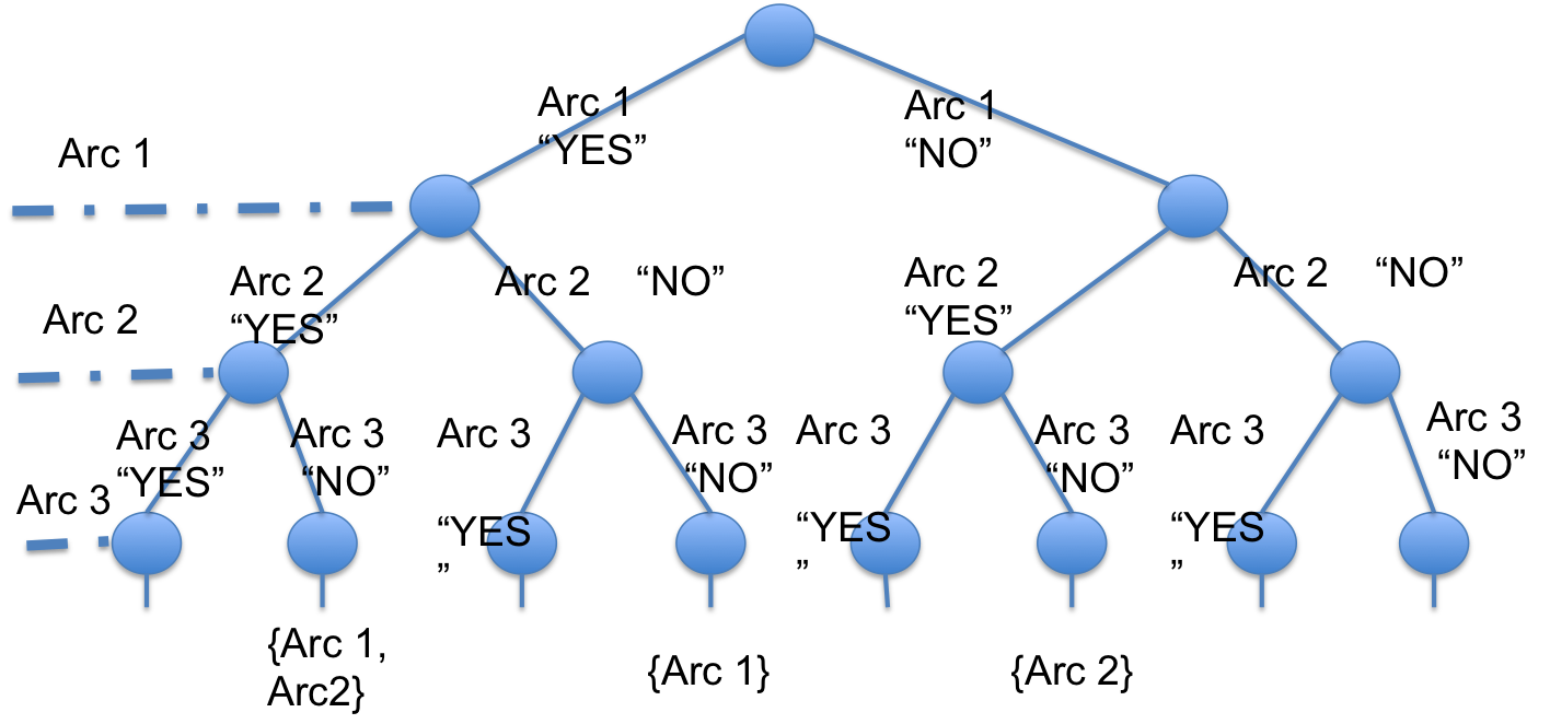
Figure 3: Tree-like representation of the Max-profit Balanced Settlement search space considered in the Settle-bb algorithm.

Algorithm 1 Settle-bb

0:  An R-multigraph $\mathcal{G}=(\mathcal{V},\mathcal{E},w)$

0:  A multiset $\mathcal{E}^{*}\subseteq\mathcal{E}$

1:  $\mathcal{T}:=\mbox{tree-like representation of }2^{\mathcal{E}}$

2:  $\mathcal{X}\leftarrow\{\mbox{root of }\mathcal{T}\}$,   $LB_{max}\leftarrow 0$

3:  while $\mathcal{X}\mbox{ contains some non-leaf tree-nodes}$ do

4:     $X\leftarrow\mbox{extract (and remove) a non-leaf tree-node from }\mathcal{X}$

5:     $UB_{X}\leftarrow\mbox{upper bound on the solutions spanned by $X$}${Algortihm 3}

6:     if $UB_{X}\geq LB_{max}$ then

7:        $LB_{X}\leftarrow\mbox{lower bound on the solutions spanned by $X$}${Algorithm 2}

8:        if $LB_{X}=UB_{X}$ then

9:           $\mathcal{E}^{*}\leftarrow arcs(X)$ and stop the algorithm

10:        end if

11:        $LB_{max}\leftarrow\max\{LB_{max},LB_{X}\}$

12:        add all $X$’s children to $\mathcal{X}$

13:     end if

14:  end while

15:  $\mathcal{L}\leftarrow\{\mbox{leaf }X\!\in\!\mathcal{X}\!\mid\!\mbox{$arcs(X)$ meet Problem~{}\ref{problem:balancestatic}'s constraints}\}$

16:  $\mathcal{E}^{*}\leftarrow\operatorname*{arg\,max}_{arcs(X):X\in\mathcal{L}}\sum_{e\in arcs(X)}w(e)$

Lower bound. For a tree-node $X$ at level $i$ of $\mathcal{T}$, let $\mathcal{E}_{X}$ denote the arcs for which a decision has been taken, i.e., arcs corresponding to all levels from the root to level $i$. Let also $\mathcal{E}_{X}$ be partitioned into $\mathcal{E}^{+}_{X}$ and $\mathcal{E}^{-}_{X}$, i.e., arcs included and not included in the current (partial) solution. A lower bound on the solutions spanned by (the subtree rooted in) $X$ can be defined by computing any feasible solution $\hat{\mathcal{E}}$ to Max-profit Balanced Settlement, subject to the additional constraint of containing all arcs in $\mathcal{E}^{+}_{X}$ and no arcs in $\mathcal{E}^{-}_{X}$.

To compute such a feasible solution, we aim at finding the set $\mathscr{C}$ of cycles of the multigraph induced by the arc set $\mathcal{E}\setminus\mathcal{E}^{-}_{X}$, and greedily selects cycles based on their amount, as long as they meet Constraint (2) of Max-profit Balanced Settlement. The intuition behind this strategy is twofold. First, a solution composed of a set of cycles always satisfies the other constraint of the problem, as every node of a cycle has at least one incoming arc and one outgoing arc. Moreover, cycle enumeration is a well-known problem, for which a variety of algorithms exists. As a trade-off between effectiveness, efficiency and simplicity, we employ a variant of the classic Johnson’s algorithm [14], in particular the version that works on multigraphs [12].

More in detail, the algorithm at hand is dubbed Settle-bb-lb and outlined as Algorithm 2. To guarantee the inclusion of the arcs $\mathcal{E}_{X}^{+}$, the greedy cycle-selection step (Lines 8–11) is preceded by a covering phase (Lines 3–7), whose goal is to find a first subset $\hat{\mathscr{C}}\subseteq\mathscr{C}$ of cycles that ($i$) cover all arcs in $\mathcal{E}_{X}^{+}$, i.e., $\mathcal{E}_{X}^{+}\subseteq\bigcup_{C\in\hat{\mathscr{C}}}C$, ($ii$) maximize the total amount of the cycle set, i.e., $\sum_{e\in\bigcup_{C\in\hat{\mathscr{C}}}C}w(e)$, and ($iii$) remain feasible for Max-profit Balanced Settlement. This corresponds to a variant of the well-known Weighted Set Cover problem, where $\mathcal{E}_{X}^{+}$ represents the universe of elements, while the cycles in $\mathscr{C}$ represent the covering sets. The covering phase of Settle-bb-lb is therefore tackled by adapting the classic greedy $(1+\log|\mathcal{E}_{X}^{+}|)$-approximation algorithm [7] for Weighted Set Cover, which iteratively selects the set minimizing the ratio between the set cost and the number of uncovered elements within that set, until all elements have been covered. Our adaptation consists in ($i$) defining the cost of a set as the inverse of the amount of the corresponding cycle (computed by discarding arcs already part of the output solution), and ($ii$) checking whether the Max-profit Balanced Settlement constraints are satisfied while selecting a cycle. In the event that not all arcs in $\mathcal{E}_{X}^{+}$ have been covered, the algorithm returns an empty set (and the lower bound used in Settle-bb is set to zero).

Algorithm 2 Settle-bb-lb

0:  An R-multigraph $\mathcal{G}=(\mathcal{V},\mathcal{E},w)$, two multisets $\mathcal{E}_{X}^{+}\subseteq\mathcal{E}$, $\mathcal{E}_{X}^{-}\subseteq\mathcal{E}$

0:  A multiset $\hat{\mathcal{E}}\subseteq\mathcal{E}\setminus\mathcal{E}^{-}_{X}$

1:  $\mathscr{C}\leftarrow\mbox{cycles of multigraph }\mathcal{G}^{-}=(\mathcal{V},\mathcal{E}\setminus\mathcal{E}_{X}^{-},w)${cf. [12]}

2:  $\hat{\mathcal{E}}\leftarrow\emptyset$,   $\hat{\mathscr{C}}\leftarrow\emptyset$

3:  while $\mathscr{C}\neq\emptyset\wedge\mathcal{E}^{+}_{X}\nsubseteq\hat{\mathcal{E}}$ do

4:     $\mathscr{C}\leftarrow\{\mbox{$C\in\mathscr{C}\mid\hat{\mathcal{E}}\cup C$ meets Constraint~{}(\ref{eq:prob1constraint1}) of Problem~{}\ref{problem:balancestatic}}\}$

5:     $C\leftarrow\mbox{cycle in $\mathscr{C}$ minimizing $[|C\!\cap\!(\mathcal{E}^{+}_{X}\setminus\hat{\mathcal{E}})|\!\sum_{e\in C\setminus\hat{\mathcal{E}}}w(e)]^{-1}$}$

6:     $\hat{\mathscr{C}}\leftarrow\hat{\mathscr{C}}\cup\{C\}$,   $\mathscr{C}\leftarrow\mathscr{C}\setminus\{C\}$,   $\hat{\mathcal{E}}\leftarrow\hat{\mathcal{E}}\cup C$

7:  end while

8:  while $\mathscr{C}\neq\emptyset$ do

9:     $\mathscr{C}\leftarrow\{\mbox{$C\in\mathscr{C}\mid\hat{\mathcal{E}}\cup C$ meets Constraint~{}(\ref{eq:prob1constraint1}) of Problem~{}\ref{problem:balancestatic}}\}$

10:     $C\leftarrow\mbox{cycle in $\mathscr{C}$ maximizing $\sum_{e\in C\setminus\hat{\mathcal{E}}}w(e)$}$

11:     $\mathscr{C}\leftarrow\mathscr{C}\setminus\{C\}$,   $\hat{\mathcal{E}}\leftarrow\hat{\mathcal{E}}\cup C$

12:  end while

13:  if $\mathcal{E}^{+}_{X}\nsubseteq\hat{\mathcal{E}}$ then

14:     $\hat{\mathcal{E}}\leftarrow\emptyset$

15:  end if

Time complexity: The running time of Settle-bb-lb is dominated by cycle enumeration (Line 2), as the number of cycles in a (multi)graph can be exponential. In our context this is however not blocking: as it is unlikely that the problem constraints are satisfied on long cycles, we employ a simple yet effective workaround of detecting cycles up to a certain size $L$. The complexity of the remaining steps is as follows. The covering phase (Lines 3–6) can be implemented by using a priority queue with logarithmic-time insertion/extraction. It comprises: ($i$) computing set-cover score and checking the problem constraints for all cycles ($\mathcal{O}(L~{}\!|\mathscr{C}|)$ time); ($ii$) adding/extracting cycles to/from the queue ($\mathcal{O}(|\mathscr{C}|\log|\mathscr{C}|)$ time); ($iii$) once a cycle $C$ has been processed, updating the score of all cycles sharing some edges with $C$ ($\mathcal{O}(L~{}\!|\mathscr{C}|\log|\mathscr{C}|)$ time, as each cycle is updated at most $L$ times, and, for every time, it should be removed from the queue and re-added with updated score). Hence, the covering phase takes $\mathcal{O}(L~{}\!|\mathscr{C}|\log|\mathscr{C}|)$ time. In greedy selection (Lines 7–11) cycles are processed one by one in non-increasing amount order, and added to the solution after checking (in $\mathcal{O}(L)$ time) the problem constraints. This yields a $\mathcal{O}(|\mathscr{C}|~{}\!(\log|\mathscr{C}|+L))$ time.

Upper bound. The Settle-bb upper bound lies on a relaxation of Max-profit Balanced Settlement where Constraint (2) is discarded and arcs are allowed to be selected fractionally:

Problem 2 (Relaxed Settlement)

Given an R-multigraph $\mathcal{G}=(\mathcal{V},\mathcal{E},w)$, find $\mbox{ }\{x_{e}\in[0,1]\}_{e\in\mathcal{E}}$ so as to

$$\begin{array}[]{rl}\mbox{Maximize}&\sum_{e\in\mathcal{E}}x_{e}w(e)\\ \mbox{subject to}&\big{(}\sum_{e=(v,u)\in\mathcal{E}}x_{e}w(e)-\sum_{e=(u,v)\in\mathcal{E}}x_{e}w(e)\big{)}\\ &\in\left[fl(u)\!-\!bl_{a}(u),cap(u)\!-\!bl_{r}(u)\right],\ \ \forall u\in\mathcal{V}\end{array}$$

The desired upper bound relies on an interesting characterization of Relaxed Settlement as a network-flow problem. As a major result in this regard, we show that solving Relaxed Settlement on multigraph $\mathcal{G}$ is equivalent to solving the well-established Min-Cost Flow problem [1] on an ad-hoc modified version of $\mathcal{G}$. We start by recalling the Min-Cost Flow problem:

Problem 3 (Min-Cost Flow [1])

Given a simple directed graph $G=(V,E)$, a cost function $c:E\rightarrow\mathds{R}$, lower-bound and upper-bound functions $\lambda:E\rightarrow\mathds{R}$, $\mu:E\rightarrow\mathds{R}$, and a supply/demand function $b:V\rightarrow\mathds{R}$, find a flow $f:E\rightarrow\mathds{R}$ so as to

$$\begin{array}[]{rl}\mbox{Minimize}&\!\!\sum_{e\in E}c(e)f(e)\\ \mbox{subject to}&\!\!\lambda(e)\leq f(e)\leq\mu(e),\ \ \forall e\in E\\ &\!\!\!\!\!\!\!\!\!\!\!\!\!\!\!\!\!\!\!\sum_{u:(v,u)\in E}f(v,u)\!-\!\sum_{u:(u,v)\in E}f(u,v)=b(u),\forall u\in V\end{array}$$

The modified version of $\mathcal{G}$ considered in this context is as follows:

Definition 2 (R-flow graph)

The R-flow graph $\mathcal{G}_{f}=(\mathcal{V}_{f},\mathcal{E}_{f},w_{f})$ of an R-multigraph $\mathcal{G}=(\mathcal{V},\mathcal{E},w)$ is a simple weighted directed graph where:

• All arcs $(u,v)\in\mathcal{E}$ between the same pair of nodes are collapsed into a single one, and the weight $w_{f}(u,v)$ is set to $\sum_{(u,v)\in\mathcal{E}}w(u,v)$;

• $\mathcal{V}_{f}=\mathcal{V}\cup\{\tilde{s},\tilde{t}\}$, i.e., the node set of $\mathcal{G}_{f}$ is composed of all nodes of $\mathcal{G}$ along with two dummy nodes $\tilde{s}$ and $\tilde{t}$;

• $\mathcal{E}_{f}=\mathcal{E}\cup\{(\tilde{s},u)\mid u\in\mathcal{V}\}\cup\{(u,\tilde{t})\mid u\in V\}\cup\{(\tilde{t},\tilde{s})\}$, i.e., the arc set of $\mathcal{G}_{f}$ is composed of ($i$) all (collapsed) arcs of $\mathcal{G}$, ($ii$) for each node $u\in\mathcal{V}$, a dummy arc $(\tilde{s},u)$ with weight $w_{f}(\tilde{s},u)\!=\!bl_{a}(u)\!-\!fl(u)$ and a dummy arc $(u,\tilde{t})$ with weight $w_{f}(u,\tilde{t})\!=\!cap(u)\!-\!bl_{r}(u)$, and ($iii$) a dummy arc $(\tilde{t},\tilde{s})$ with weight $w_{f}(\tilde{t},\tilde{s})\!=\!\infty$.

The main result for the computation of the desired upper bound is stated in the next theorem and corollary:

Theorem 2

Given an R-multigraph $\mathcal{G}=(\mathcal{V},\mathcal{E},w)$, let $\mathcal{G}_{f}=(\mathcal{V}_{f},\mathcal{E}_{f},w_{f})$ be the R-flow graph of $\mathcal{G}$. Let also cost, lower-bound, upper-bound and supply/demand functions $c:\mathcal{E}_{f}\rightarrow\mathds{R}$, $\lambda:\mathcal{E}_{f}\rightarrow\mathds{R}$, $\mu:\mathcal{E}_{f}\rightarrow\mathds{R}$ and $b:\mathcal{V}_{f}\rightarrow\mathds{R}$ be defined as:

• $\lambda(e)=0$, $\mu(e)=w_{f}$,  $\forall e\in\mathcal{E}_{f}$;

• $c(\tilde{t},\tilde{s})=0$, and $c(\tilde{s},u)=c(u,\tilde{t})=0$,  $\forall u\in\mathcal{V}_{f}$;

• $c(e)=-1$,  $\forall e\in\mathcal{E}_{f}\cap\mathcal{E}$;

• $b(u)=0$,  $\forall u\in\mathcal{V}_{f}$.

It holds that solving Min-Cost Flow on input $\langle\mathcal{G}_{f},c,\lambda,\mu,b\rangle$ is equivalent to solving Relaxed Settlement on input $\mathcal{G}$.

Proof:

As $c(e)=-1$, if $e\in\mathcal{E}$, $c(e)=0$, otherwise, and $\forall e\in\mathcal{E}:0\leq f(e)\leq w(e)$, the objective function of Min-Cost Flow on $\mathcal{G}_{f}$ can be rewritten as $\min\sum_{e\in\mathcal{E}}-f(e)$, which is equivalent to the objective $\max\sum_{e\in\mathcal{E}}x_{e}w(e)$ ($x_{e}\in[0,1]$) of Relaxed Settlement on $\mathcal{G}$. For the cap-floor constraints, the conservation of flows ensures for any solution to Min-Cost Flow on $\mathcal{G}_{f}$:

$$\begin{array}[]{l}\forall u\in\mathcal{V}:\\ \sum_{(v,u)\in\mathcal{E}}\!f(v,u)\!+\!f(\tilde{s},u)\!-\!\sum_{(u,v)\!\in\mathcal{E}}\!f(u,v)\!-\!f(u,\tilde{t})\!=\!b(u)\!=\!0\\ \!\!\!\Leftrightarrow\!\forall u\!\in\!V\!:\!\!\sum_{(v,u)\in\mathcal{E}}f(v,u)-\sum_{(u,v)\in\mathcal{E}}f(u,v)=f(u,\tilde{t})-f(\tilde{s},u).\end{array}$$

As $f(\tilde{s},u)\in[f_{min}(\tilde{s},u),f_{max}(\tilde{s},u)]=[0,bl_{a}(u)\!-\!fl(u)]$ and $f(u,\tilde{t})\in[f_{min}(u,\tilde{t}),f_{max}(u,\tilde{t})]=[0,cap(u)\!-\!bl_{r}(u)]$, then:

$$\begin{array}[]{l}\forall u\in\mathcal{V}:\sum_{(v,u)\in\mathcal{E}}f(v,u)-\sum_{(u,v)\in\mathcal{E}}f(u,v)\\ =f(u,\tilde{t})-f(\tilde{s},u)\leq f_{max}(u,\tilde{t})-f_{min}(\tilde{s},u)\\ =cap(u)-bl_{r}(u),\end{array}$$

and

$$\begin{array}[]{l}\forall u\in\mathcal{V}:\sum_{(v,u)\in\mathcal{E}}f(v,u)-\sum_{(u,v)\in\mathcal{E}}f(u,v)\\ =f(u,\tilde{t})-f(\tilde{s},u)\geq f_{min}(u,\tilde{t})-f_{max}(\tilde{s},u)\\ =fl(u)-bl_{a}(u).\end{array}$$

Overall, it is therefore guaranteed that $\forall u\in\mathcal{V}$:

$$\sum_{(v,u)\in\mathcal{E}}\!\!\!f(v,u)-\!\!\!\!\sum_{(u,v)\in\mathcal{E}}\!\!f(u,v)\in[fl(u)-bl_{a}(u),cap(u)-bl_{r}(u)],$$

i.e., the floor-cap constraints in Relaxed Settlement. ∎

Corollary 1

Given an R-multigraph $\mathcal{G}$, the solution to Max-profit Balanced Settlement on $\mathcal{G}$ is upper-bounded by the solution to Min-Cost Flow on the input $\langle\mathcal{G}_{f},c,\lambda,\mu,b\rangle$ of Theorem 2.

Proof:

Immediate as, according to Theorem 2, the solution to Min-cost Flow on input $\langle\mathcal{G}_{f},c,\lambda,\mu,b\rangle$ corresponds to the optimal solution to a relaxed version of the Max-profit Balanced Settlement problem on the original R-multigraph $\mathcal{G}$. ∎

Algorithm 3 Settle-bb-ub

0:  An R-multigraph $\mathcal{G}=(\mathcal{V},\mathcal{E},w)$, two multisets $\mathcal{E}_{X}^{+}\subseteq\mathcal{E}$, $\mathcal{E}_{X}^{-}\subseteq\mathcal{E}$

0:  A real number $UB_{X}$

1:  $\!\mathcal{G}^{-}:=(\mathcal{V},\mathcal{E}\setminus\mathcal{E}_{X}^{-},w)$

2:  $UB_{X}\!\leftarrow\!\mbox{solve {Min-Cost Flow} applying Theorem~{}\ref{theorem:flow}}$ on $\mathcal{G}^{-}\!$ and forcing flow $f(e)=w(e)$, $\forall e\in\mathcal{E}_{X}^{+}$; return $-\!1$ if no admissible solution exists

Corollary 1 is exploited for upper-bound computation as in Algorithm 3. To handle the arcs to be discarded ($\mathcal{E}^{-}$) and included ($\mathcal{E}^{+}$), Algorithm 3 removes all arcs $\mathcal{E}^{-}$ from the multigraph, and asks for a Min-Cost Flow solution where the flow on every arc $e\in E^{+}$ is forced to be $w(e)$. If no solution satisfying such a requirement exists, no admissible solution to Max-profit Balanced Settlement exists in the entire subtree rooted in the target tree-node $X$. In this case the returned upper bound is $-1$, and the subtree rooted in $X$ is pruned by the Settle-bb algorithm. We solve Min-Cost Flow with the well-established Cost Scaling algorithm [10], which has $\mathcal{O}(|\mathcal{E}|~{}\!(|\mathcal{V}|\log|\mathcal{V}|)~{}\!\log(|\mathcal{V}|~{}\!w_{max}))$ time complexity, where $w_{max}=\max_{e\in\mathcal{E}}w(e)$. This also corresponds to the time complexity of the entire upper-bound computation method.

4.2 Beam-search algorithm

Being Max-profit Balanced Settlement $\mathbf{NP}$-hard, the exact Settle-bb algorithm cannot handle large R-multigraphs. We thus design an alternative algorithm that finds approximate solutions and can run on larger instances. To this end, we exploit the idea of enumerating all cycles in the input multigraph, and selecting a subset of them while keeping the constraints satisfied. The intuition behind this strategy is twofold. First, a solution composed of a set of cycles always satisfies the other constraint of the problem, as every node of a cycle has at least one incoming arc and one outgoing arc. Also, cycle enumeration is a well-established problem, for which a variety of algorithms exist. As a trade-off between effectiveness, efficiency and simplicity, in this work we employ a variant of the Johnson’s algorithm [14] that works on multigraphs [12].

Optimal cycle selection. For a principled cycle selection, we focus on the problem of seeking cycles that satisfy the constraints in Problem 1 and exhibit maximum total amount:

Problem 4 (Optimal Cycle Selection)

​​​Given an R-multigraph $\mathcal{G}\!=\!(\mathcal{V},\mathcal{E},w)$ and a set $\mathscr{C}$ of cycles in $\mathcal{G}$, find a subset $\mathscr{C}^{*}\!\subseteq\!\mathscr{C}$ so that:

$$\vspace{-1mm}\begin{array}[]{rl}\!\!\!\!\!\!\!\!\!\!\!\!\mathscr{C}^{*}=&\!\!\!\arg\max_{\hat{\mathscr{C}}\subseteq\mathscr{C}}\sum_{e\in\mathcal{E}(\hat{\mathscr{C}})}w(e)\\ \!\!\!\!\!\!\!\!\!\!\!\!\mbox{subject to}&\!\!\!\mbox{$\mathcal{E}(\hat{\mathscr{C}})\!=\!\bigcup_{C\in\hat{\mathscr{C}}}C$ meets Constraint~{}(\ref{eq:prob1constraint1}) in Problem~{}\ref{problem:balancestatic}}.\end{array}$$

Theorem 3

Problem 4 is $\mathbf{NP}$-hard.

Proof:

We reduce from Maximum Independent Set [8], which asks for a maximum-sized subset of vertices in a graph no two of which are adjacent. Given a graph $G=(V,E)$ instance of Maximum Independent Set, we construct an instance $\langle\mathcal{G},\mathscr{C}\rangle$ of Optimal Cycle Selection as follows. For a vertex $u\in V$, let $N(u)=\{v\mid(u,v)\in E\}$, $d_{u}=|N(u)|$, $d_{max}=\max_{u\in V}d_{u}$. Without loss of generality, we assume that $\forall u\in V:d_{u}>0$. First, we let the node set $\mathcal{V}$ of $\mathcal{G}$ contain: ($i$) a pair of nodes $\langle u^{\prime},u^{\prime\prime}\rangle$ for every vertex $u\in V$, ($ii$) a node $uv$ for each $(u,v)\in E$. Let also $\mathcal{V}$ follow a global ordering. For each $u\in V$, we create a cycle $C_{u}=c_{1}\rightarrow c_{2}\rightarrow\cdots\rightarrow c_{d_{u}+2}\rightarrow c_{1}$ in $\mathcal{G}$, where $c_{1}=u^{\prime}$, $c_{2}=u^{\prime\prime}$, and all other nodes $c_{i}:i>2$ correspond to nodes $\{uv\in\mathcal{V}\mid v\in N(u)\}$, ordered as picked above. The arc weights of $C_{u}$ are defined as follows:

• $w(c_{1},c_{2})=1+\frac{3}{2}[d_{max}(d_{max}+1)-d_{u}(d_{u}+1)]$,

• $w(c_{i},c_{i+1})=d_{u}+i-2$, $\forall i\in[2..d_{u}+1]$,

• $w(c_{d_{u}+2},c_{1})=2d_{u}$.

Finally, we set

• $bl_{r}(x)=bl_{a}(x)=0$,  $cap(x)=+\infty$,  $\forall x\in\mathcal{V}$,

• $fl(u^{\prime})=fl(u^{\prime\prime})=-\infty$, $\forall u^{\prime},u^{\prime\prime}$,

• $fl(uv)=-1$, $\forall uv$,

and the input cycles $\mathscr{C}$ equal to $\{C_{u}\mid u\in V\}$. It holds that:

1. $\mathcal{G}$ has $2|V|\!+\!|E|$ nodes and $\sum_{u\in V^{\prime}}(d_{u}\!+\!2)=2(|V|\!+\!|E|)$ arcs, taking polynomial space and construction time in the $G$’s size.

2. All cycles in $\mathscr{C}$ are arc-disjoint with respect to each other.

3. Every cycle $C_{u}\in\mathscr{C}$ has the same total amount, which is equal to $1+\frac{3}{2}[d_{max}(d_{max}+1)-d_{u}(d_{u}+1)]$ $+\sum_{i=0}^{d_{u}}(d_{u}+i)$ $=1+\frac{3}{2}[d_{max}(d_{max}\!+\!1)-d_{u}(d_{u}\!+\!1)]+\frac{3}{2}d_{u}(d_{u}+1)$ $\!=\!1+\frac{3}{2}d_{max}(d_{max}\!+\!1)$.

4. Selecting any two cycles $C_{u},C_{v}\in\mathscr{C}$ such that $u$ and $v$ are adjacent in $G$, violates the constraint on $fl(uv)$ (as $bl_{a}(uv)$ will result to be $bl_{a}(uv)=-2<fl(uv)=-1)$).

Based on (b) and (c), any cycle brings the same gain to the objective. Thus, solving Optimal Cycle Selection on $\langle\mathcal{G},\mathscr{C}\rangle$ corresponds to selecting the maximum number of cycles in $\mathscr{C}$ so that cap-floor constraints are met. Combined with (d), solving Optimal Cycle Selection on $\langle\mathcal{G},\mathscr{C}\rangle$ is equivalent to selecting the maximum number of vertices in $G$ no two of which are adjacent. ∎

Algorithm 4 Settle-beam

0:  R-multigraph $\mathcal{G}=(\mathcal{V},\mathcal{E},w)$,  integer $K$

0:  Multiset $\mathcal{E}^{*}\subseteq\mathcal{E}$

1:  $\mathcal{E}^{*}\leftarrow\emptyset$

2:  $\mathscr{C}\leftarrow\mbox{cycles of }\mathcal{G}$ {[12]}

3:  while $\mathscr{C}\neq\emptyset$ do

4:     $\mathscr{C}^{\prime}\leftarrow\mbox{$K$-sized subset of $\mathscr{C}$ by {Greedy} {Max Cover}}${[13]}

5:     $\mathscr{C}^{\prime}_{2}\leftarrow\{\{C_{i},C_{j}\}\!\mid\!C_{i},C_{j}\in\mathscr{C}^{\prime}\}$

6:     for all $\{C_{i},C_{j}\}\in\mathscr{C}^{\prime}_{2}$ do

7:        $C_{ij}\leftarrow C_{i}\cup C_{j}$

8:        process all $C\!\in\!\mathscr{C}^{\prime}\!\setminus\!\{C_{i},C_{j}\}$ one by one, by non-increasing $\omega(\cdot)$ score (Eq.(3)); add $C$ to $C_{ij}$ if $C_{ij}\cup C\cup\mathcal{E}^{*}$ is feasible for Problem 4

9:     end for

10:     $\mathcal{E}^{*}\leftarrow\mathcal{E}^{*}\cup\arg\max_{C_{ij}\in\mathscr{C}^{\prime}_{2}}\sum_{e\in C_{ij}}w(e)$

11:     $\mathscr{C}\leftarrow\mathscr{C}\setminus(\mathscr{C}^{\prime}\cup\{C\in\mathscr{C}\mid C\cap\mathcal{E}^{*}=C\})$

12:  end while

Characterization as a Knapsack problem. As Optimal Cycle Selection is $\mathbf{NP}$-hard, we focus on designing effective approximated solutions. To this end, we show an intriguing connection with the following variant of the well-known Knapsack problem:

Problem 5 (Set Union Knapsack [11])

Let $U=\{x_{1},\ldots,x_{h}\}$ be a universe of elements, $\mathcal{S}=\{S_{1},\ldots,S_{k}\}$ be a set of items, where $S_{i}\subseteq U$, $\forall i\in[1..k]$, $p:\mathcal{S}\rightarrow\mathds{R}$ be a profit function for items in $\mathcal{S}$, and $q:U\rightarrow\mathds{R}$ be a cost function for elements in $U$. For any $\hat{\mathcal{S}}\subseteq\mathcal{S}$ define also: $U(\hat{\mathcal{S}})=\bigcup_{S\in\hat{\mathcal{S}}}S$, $P(\hat{\mathcal{S}})=\sum_{S\in\hat{\mathcal{S}}}p(S)$, and $Q(\hat{\mathcal{S}})=\sum_{x\in U(\hat{\mathcal{S}})}q(x)$. Given a real number $B\in\mathds{R}$, Set Union Knapsack finds  $\mathcal{S}^{*}=\arg\max_{\hat{\mathcal{S}}\subseteq\mathcal{S}}P(\hat{\mathcal{S}})\ \ \mbox{s.t.}\ \ Q(\hat{\mathcal{S}})\leq B.$

A simple variant of Set Union Knapsack arises when both costs and budget constraint are $d$-dimensional:

Problem 6 (Multidimensional Set Union Knapsack)

Given $U$, $\mathcal{S}$, $p$ as in Problem 5, a $d$-dimensional cost function $q:U\rightarrow\mathds{R}^{d}$, and a $d$-dimensional vector $\mathbf{B}\in\mathds{R}^{d}$, find $\mathcal{S}^{*}=\arg\max_{\hat{\mathcal{S}}\subseteq\mathcal{S}}P(\hat{\mathcal{S}})$ $\mbox{s.t.}\ \ \mathbf{Q}(\hat{\mathcal{S}})\leq\mathbf{B},$ where $\mathbf{Q}(\hat{\mathcal{S}})=\sum_{x\in U(\hat{\mathcal{S}})}q(x)$.

We observe that an instance of Optimal Cycle Selection can be transformed into an instance of Multidimensional Set Union Knapsack so that every feasible solution for the latter instance is also a feasible solution for the original Optimal Cycle Selection instance. We let the arcs $\mathcal{E}$ represent elements, cycles $\mathscr{C}$ represent items, and define $2|\mathcal{V}|$ costs/budgets for each element (arc), so as to match the cap-floor constraints on every node ($|\mathcal{V}|$ costs/budgets for cap- and floor-related constraints each). Formally:

Theorem 4

Given an R-multigraph $\mathcal{G}=(\mathcal{V},\mathcal{E},w)$ and a set $\mathscr{C}$ of cycles in $\mathcal{G}$, let $\langle U,\mathcal{S},p,q,\mathbf{B}\rangle$ be an instance of Multidimensional Set Union Knapsack defined as follows:

• $U=\mathcal{E}$;  $\mathcal{S}=\mathscr{C}$;  $\forall C\in\mathscr{C}:p(C)=\sum_{e\in C}w(e)$;

• $\forall(u_{i},u_{j})\!\in\!\mathcal{E}:q(u_{i},u_{j})\!=\![\mathbf{q}^{+}(u_{i},u_{j})~{}\!\mathbf{q}^{-}(u_{i},u_{j})]\!\in\!\mathds{R}^{2|\mathcal{V}|}$, where

  • $\mathbf{q}^{+}(u_{i},u_{j})=[q^{+}_{k}(u_{i},u_{j})]_{k=1}^{|\mathcal{V}|}$, with $q^{+}_{i}(u_{i},u_{j})=-w(u_{i},u_{j})$, $q^{+}_{j}(u_{i},u_{j})=w(u_{i},u_{j})$, and $q^{+}_{k}(u_{i},u_{j})=0$, for $k\neq i,j$;

  • $\mathbf{q}^{-}(u_{i},u_{j})=[q^{-}_{k}(u_{i},u_{j})]_{k=1}^{|\mathcal{V}|}$, with $q^{-}_{i}(u_{i},u_{j})=w(u_{i},u_{j})$,
    $q^{-}_{j}(u_{i},u_{j})~{}=~{}-w(u_{i},u_{j})$, and $q^{-}_{k}(u_{i},u_{j})=0$, for $k\neq i,j$;

• $\mathbf{B}:=[\mathbf{B}^{+}\ \mathbf{B}^{-}]\in\mathds{R}^{2|\mathcal{V}|}$, where

  • $\mathbf{B}^{+}=[cap(u_{1})-bl_{r}(u_{1}),\ldots,cap(u_{n})-bl_{r}(u_{n})]$;

  • $\mathbf{B}^{-}=[bl_{a}(u_{1})-fl(u_{1}),\ldots,bl_{a}(u_{n})-fl(u_{n})]$.

It holds that any feasible solution for Multidimensional Set Union Knapsack on input $\langle U,\mathcal{S},p,q,\mathbf{B}\rangle$ is a feasible solution for Optimal Cycle Selection on input $\langle\mathcal{G},\mathscr{C}\rangle$.

Proof:

(Sketch) It suffices to show that the constraints of Multidimensional Set Union Knapsack on $\langle U,\mathcal{S},p,q,\mathbf{B}\rangle$ correspond to cap-floor constraints of Optimal Cycle Selection on $\langle\mathcal{G},\mathscr{C}\rangle$. This can be achieved by simple math on $\mathbf{q}^{+}$​​, $\mathbf{q}^{-}$​​, $\mathbf{B}^{+}$​​, $\mathbf{B}^{-}$​​. ∎

Putting it all together. Motivated by Theorem 4, we devise an algorithm to approximate Optimal Cycle Selection inspired by Arulselvan’s algorithm for Set Union Knapsack [3], which achieves a $1\!-\!e^{-1/f_{max}}$ approximation guarantee, where $f_{max}$ is the maximum number of items in which an element is present. Arulselvan’s algorithm considers all subsets of 2 items whose weighted union is within the budget $B$. Then, it augments each subset with items $S_{i}$ added one by one in the decreasing order of an ad-hoc-defined score, as long as the inclusion of $S_{i}$ complies with the budget constraint $B$. The score exploited for item processing is directly proportional to the profit of $S_{i}$ and inversely proportional to the frequency of $S_{i}$’s elements within the entire item set $\mathcal{S}$. The highest-profit one of such augmented subsets is returned as output.

The ultimate Settle-beam algorithm (Algorithm 4) combines the ideas behind Arulselvan’s algorithm with the beam-search paradigm and a couple of adaptations to make it suitable for our context. Particularly, the adaptations are as follows. ($i$) We extend Arulselvan’s algorithm so as to handle a Multidimensional Set Union Knapsack problem instance derived from the input Optimal Cycle Selection instance as stated in Theorem 4 (trivial extension). ($ii$) We define the score of a cycle $C\in\mathscr{C}$ as:

$$\omega(C)=\frac{\sum_{e\in C}w(e)}{\sum_{e\in C}\frac{w(e)}{f(e)}},\ \mbox{where }f(e)=|\{C\in\mathscr{C}:e\in C\}|,\vspace{-1mm}$$ (3)

whose rationale is to consider the total cycle amount, penalized by a term accounting for the frequency of an arc within the whole cycle set $\mathscr{C}$. The idea is that frequent arcs contribute less to the objective function, which is defined on the union of the arcs of all selected cycles (see Problem 4). Finally, ($iii$) to overcome the expensive pairwise cycle enumeration and augmentation of all 2-sized cycle sets with all other cycles, we adopt a beam-search methodology to reduce the cycles to be considered. We first select a subset $\mathscr{C}^{\prime}\subseteq\mathscr{C}$ of cycles of size $K\leq|\mathscr{C}|$ whose union arc set exhibits the maximum amount, and use $\mathscr{C}^{\prime}$ for both pairwise cycle computation and augmentation. We repeat the procedure (by selecting a further $K$-sized subset of $\mathscr{C}\setminus\mathscr{C}^{\prime}$) until $\mathscr{C}$ has become empty.

Time complexity. As far as cycle enumeration, the considerations made for Algorithm 2 (Section 4.1) remain valid here too. The complexity of the remaining main steps is as follows. Denoting by $L$ the maximum size of a cycle in $\mathscr{C}$, the greedy Max Cover algorithm on input $\mathscr{C}^{\prime}$ (Line 4) takes $\mathcal{O}(L~{}\!K\log K)$ time. All feasible cycle pairs (Line 5) can be computed in $\mathcal{O}(L~{}\!K^{2})$ time, while augmentation of all such pairs (Lines 6–8) takes $\mathcal{O}(L~{}\!K^{3})$ time. All these steps are repeated $\mathcal{O}(\frac{|\mathscr{C}|}{K})$ times. The overall time complexity is $\mathcal{O}(L~{}\!K^{2}~{}\!|\mathscr{C}|)$.

Algorithm 5 Settle-path

0:  R-multigraph $\mathcal{G}=(\mathcal{V},\mathcal{E},w)$,  two integers $K,K_{p}$

0:  Multiset $\mathcal{E}^{*}\subseteq\mathcal{E}$

1:  $\mathscr{C}^{*}\leftarrow$ cycles of $\mathcal{G}$ selected by Algorithm 4

2:  $\mathcal{E}^{*}\leftarrow\bigcup_{C\in\mathscr{C}^{*}}C$

3:  for all $C_{i},C_{j}\in\mathscr{C}^{*}$ do

4:     $\mathscr{P}_{ij}\leftarrow$ paths from a node in $C_{i}$ to a node in $C_{j}${[12]}

5:     $\mathscr{P}_{ij}^{*}\leftarrow$ paths selected by Algorithm 4 on input $\langle\mathcal{G},K_{p}\rangle$ and setting $\mathscr{C}:=\mathscr{P}_{ij}$ at Line 2

6:     $\mathcal{E}^{*}\leftarrow\mathcal{E}^{*}\cup\bigcup_{P\in\mathscr{P}^{*}_{ij}}P$

7:  end for

4.3 Adding paths between cycles

An interesting insight on cycle-based solutions to Max-profit Balanced Settlement is that they can be improved by looking for paths connecting two selected cycles. An approach based on this observation is particularly appealing as adding a path between two cycles keeps the cycle constraint of our problem (i.e., Constraint (2) in Problem 1) satisfied, therefore one has only to focus on the floor-cap constraint while checking admissibility of paths.

Within this view, we propose a refinement of the Settle-beam algorithm where, for every pair $C_{i},C_{j}$ of selected cycles, we ($i$) compute paths $\mathscr{P}_{ij}$ from a node in $C_{i}$ to a node in $C_{j}$, and ($ii$) take a subset $\mathscr{P}^{*}_{ij}\subseteq\mathscr{P}_{ij}$ such that the total amount $\sum_{e\in P,P\in\mathscr{P}^{*}_{ij}}w(e)$ is as large as possible and adding $\mathscr{P}^{*}_{ij}$ to the initial Max-profit Balanced Settlement solution still meets the cap-floor constraints. We dub this algorithm Settle-path and outline it as Algorithm 5. To compute a path set $\mathscr{P}_{ij}$, we employ a simple variant of the (multigraph version of the) well-known Johnson’s algorithm [12], where we make the underlying backtracking procedure start from nodes in $C_{i}$ and yield a solution (i.e., a path) every time it encounters a node in $C_{j}$. The selection of $\mathscr{P}^{*}_{ij}\subseteq\mathscr{P}_{ij}$ can be accomplished by running either a standard greedy method (as in Algorithm 2 in the first version of our work [4]), or Algorithm 4 (with the modification that the set $\mathscr{C}$ at Line 2 corresponds to $\mathscr{P}_{ij}$).

The running time of Settle-path is expected to be dominated by the various path-enumeration steps. As far as the remaining steps, the worst case corresponds to employing Algorithm 4 for both cycle- and path-selection, which leads to an overall time complexity of $\mathcal{O}(LK^{2}|\mathscr{C}|+|\mathscr{C}^{*}|^{2}L_{p}K_{p}^{2}|\mathscr{P}_{max}|)$, where $L_{p}$ and $K_{p}$ are two integers playing the same roles as $L$ and $K$, respectively, in Algorithm 4 when run on path sets, and $\mathscr{P}_{max}=\operatorname*{arg\,max}_{\mathscr{P}\in\{\mathscr{P}_{ij}\}_{i,j}}|\mathscr{P}|$.

4.4 Hybrid algorithm

The Max-profit Balanced Settlement problem can be solved by running any of the algorithms presented in Sections 4.1–4.3 on each weakly connected component of the input R-multigraph separately, and then taking the union of all partial solutions. Based on this straightforward observation, we ultimately propose a hybrid algorithm, which runs the exact Settle-bb algorithm on the smaller connected components and the Settle-beam or Settle-path algorithm on the remaining ones.

Our hybrid algorithm is outlined as Algorithm 6: we term it either Settle-h or Settle-h-path, depending on whether it is equipped with Settle-beam or Settle-path, respectively.

Algorithm 6 Settle-h/Settle-h-path

0:  R-multigraph $\mathcal{G}=(\mathcal{V},\mathcal{E},w)$,  three integers $H,K,K_{p}$

0:  Multiset $\mathcal{E}^{*}\subseteq\mathcal{E}$

1:  $\mathcal{E}^{*}\leftarrow\emptyset$,   $\mathbf{CC}\leftarrow\mbox{weakly connected components of }\mathcal{G}$

2:  for all $G\in\mathbf{CC}$ s.t. $|arcs(G)|\leq H$ do

3:     $\mathcal{E}^{*}\leftarrow\mathcal{E}^{*}\cup$ Settle-bb on input $G${Section 4.1}

4:  end for

5:  for all $G\in\mathbf{CC}$ s.t. $|arcs(G)|>H$ do

6:     $\mathcal{E}^{*}\leftarrow\mathcal{E}^{*}\cup$ Settle-beam or Settle-path on input $\langle G,K,K_{p}\rangle${Algorithms 4–5}

7:  end for

4.5 Temporary constraint violation

Given a set $\mathcal{E}^{*}$ of receivables selected for settlement, the eventual step of our network-based RF service is, for every receivable $R\in\mathcal{E}^{*}$, to transfer $amount(R)$ from $debtor(R)$’s account to $creditor(R)$’s account. A typical desideratum from big (financial) institutions is that these money transfers happen by exploiting procedures and software solutions already in place within the institution, in order to minimize the effort in system re-engineering. For instance, our partner institution required to interpret money transfers as a sequence of standard bank transfers. To accomplish this, money transfers have to typically be executed one at a time, meaning that some constraints in Problem 1 might be temporarily violated. As an example, look at Figure 2 and assume the money transfer corresponding to the receivable from D to E is the first one to be executed: this would lead to the temporary violation of D’s floor constraint. In real scenarios constraint violation might not be allowed, not even temporarily. In banks, for instance, a floor-constraint violation corresponds to an overdraft on a bank account, which, even if it lasts a few milliseconds only, would anyway cause that account being charged. Another motivation may be simply that existing systems do not accept any form of temporary violation.

Motivated by the above, here we devise solutions to the temporary-constraint-violation issue. In particular, we focus on floor constraints only, as temporary violation of cap constraints or cycle constraints is not really critical. We propose two solutions: the first one is based on a clever redefinition of floor values, while the second one consists in properly selecting and ordering a subset of the arcs that were originally identified for settlement. The details of both solutions are reported next.

Redefining floor values. The first proposal to handle temporary constraint violation is based on the following result: properly redefining floor values leads to output solutions to Max-profit Balanced Settlement containing only receivables that do not violate the original floor constraints, regardless of the ordering with which the corresponding money transfers are executed. Specifically, given a set $\mathcal{E}^{*}\subseteq\mathcal{E}$ of arcs in a Max-profit Balanced Settlement solution, for every node $u\in\mathcal{V}(\mathcal{E}^{*})$, let $in(u,\mathcal{E}^{*})=\sum_{v:(v,u)\in\mathcal{E}^{*}}w(v,u)$ and $out(u,\mathcal{E}^{*})=\sum_{v:(u,v)\in\mathcal{E}^{*}}w(u,v)$ denote the total amount received and paid by $u$ within $\mathcal{E}^{*}$, respectively. Let also $ub_{in}(u)$ denote an upper bound on the amount $in(u,\mathcal{E}^{*})$ that $u$ can receive in any possible solution $\mathcal{E}^{*}$. Our first observation is that, by setting $fl(u)=ub_{in}(u)$, $\forall u\in\mathcal{V}(\mathcal{E}^{*})$, no customer $u$ will ever pay a total amount larger than her current $bl_{a}(u)$ balance availability $bl_{a}(u)$ in any Max-profit Balanced Settlement solution, i.e., it would be guaranteed that, for all solutions $\mathcal{E}^{*}$ and all $u\in\mathcal{V}(\mathcal{E}^{*})$, $bl_{a}(u)\geq out(u,\mathcal{E}^{*})$. In fact, for all solutions $\mathcal{E}^{*}$ it holds that:

$$in(u,\mathcal{E}^{*})-out(u,\mathcal{E}^{*})+bl_{a}(u)\ \geq\ fl(u)=ub_{in}(u)$$ (4)

$$\Leftrightarrow bl_{a}(u)-out(u,\mathcal{E}^{*})\ \geq\ ub_{in}(u)-in(u,\mathcal{E}^{*})\ \geq\ 0$$

$$\Rightarrow bl_{a}(u)\ \geq\ out(u,\mathcal{E}^{*}).$$

Now, the key question is how to define $ub_{in}(u)$. A simple way would be setting it to the $u$’s in-degree. Another option consists in defining it based on the cap constraint:

$$cap(u)\ \geq\ in(u,\mathcal{E}^{*})\!-\!out(u,\mathcal{E}^{*})\!+\!bl_{r}(u)$$

$$\Rightarrow cap(u)\ \geq\ in(u,\mathcal{E}^{*})\!-\!bl_{a}(u)\!+\!bl_{r}(u)\quad\mbox{\{Equation~{}(\ref{eqtmp1})\}}$$

$$\Leftrightarrow in(u)\ \leq\ cap(u)\!+\!bl_{a}(u)\!-\!bl_{r}(u).$$

Combining the two options, we ultimately define

$$\!ub_{in}\!(u)\!=\!\min\!\Big{\{}\!{\textstyle\sum_{v:(v,u)\in\mathcal{E}}\!w(v,\!u),cap(u)\!+\!bl_{a}\!(u)\!-\!bl_{r}\!(u)}\!\Big{\}}\!.\!\!\!\!\!$$ (5)

Algorithm 7 Redefine-Floors

0:  R-multigraph $\mathcal{G}=(\mathcal{V},\mathcal{E},w)$,  two integers $H,K$

0:  List $\mathcal{E}^{*}\subseteq\mathcal{E}$

1:  $\mathcal{E}^{*}\leftarrow[~{}\!]$

2:  repeat

3:     $\widehat{\mathcal{E}}\leftarrow$ a solution to Problem 1 on input $\langle\mathcal{G},H,K\rangle$, with floors set as $fl(u)=ub_{in}(u)$, $\forall u\in\mathcal{V}${Equation (5)}

4:     order $\widehat{\mathcal{E}}$ in some way and append it to $\mathcal{E}^{*}$

5:     remove all arcs in $\widehat{\mathcal{E}}$ from $\mathcal{G}$

6:     for all $u\in\mathcal{V}(\widehat{\mathcal{E}})$ do

7:        $\Delta(u)\leftarrow\sum_{v:(v,u)\in\widehat{\mathcal{E}}}w(v,u)-\sum_{v:(u,v)\in\widehat{\mathcal{E}}}w(u,v)$

8:        $bl_{r}(u)\leftarrow bl_{r}(u)+\Delta(u)$,  $bl_{a}(u)\leftarrow bl_{a}(u)+\Delta(u)$

9:     end for

10:  until $\mathcal{E}=\emptyset\ \vee\ \widehat{\mathcal{E}}=\emptyset$

To summarize, our first strategy to handle temporary constraint violation consists in computing a solution $\mathcal{E}^{*}$ to Max-profit Balanced Settlement with a floor constraint $fl(u)=ub_{in}(u)$ (Equation (5)), for all $u$. Based on the above arguments, $\mathcal{E}^{*}$ guarantees no temporary floor-constraint violation, independently of the execution order of the corresponding money transfers. As a refinement, one can run this method iteratively, i.e., removing the arcs yielded at any iteration and computing a new solution on the remaining graph. The overall solution is the union of all partial solutions, and the arcs are ordered based on the iterations: money transfers corresponding to arcs computed in earlier iterations should be executed before the ones in later iterations (while arc ordering within the same iteration does not matter). This method is outlined as Algorithm 7.

Algorithm 8 Select-and-Order

0:  R-multigraph $\mathcal{G}=(\mathcal{V},\mathcal{E},w)$,  two integers $H,K$

0:  List $\mathcal{E}^{*}\subseteq\mathcal{E}$

1:  $\mathcal{E}^{*}\leftarrow[~{}\!]$;   $i\leftarrow 1$

2:  repeat

3:     $\mathcal{E}^{+}\leftarrow\emptyset$

4:     for all $u\in\mathcal{V}(\mathcal{E})$ do

5:        $\mathcal{E}_{u}\leftarrow$ a subset of $\{(u,v)\mid(u,v)\in\mathcal{E}\}$ s.t. $bl_{a}(u)-\sum_{e\in\mathcal{E}_{u}}w(e)\geq fl(u)$, $\forall(u,v)\in\mathcal{E}_{u}:w(u,v)+bl_{r}(v)\leq cap(v)$, and $\sum_{e\in\mathcal{E}_{u}}w(e)$ is maximized

6:        $\mathcal{E}^{+}\leftarrow\mathcal{E}^{+}\cup\mathcal{E}_{u}$

7:     end for

8:     set $ts(e)=i$, $\forall e\in\mathcal{E}^{+}$

9:     order $\mathcal{E}^{+}$ in some way and append it to $\mathcal{E}^{*}$

10:     for all $u\in\mathcal{V}(\mathcal{E}^{+})$ do

11:        $\Delta(u)\leftarrow\sum_{v:(v,u)\in\mathcal{E}^{+}}w(v,u)-\sum_{v:(u,v)\in\mathcal{E}^{+}}w(u,v)$

12:        $bl_{r}(u)\leftarrow bl_{r}(u)+\Delta(u)$,  $bl_{a}(u)\leftarrow bl_{a}(u)+\Delta(u)$

13:     end for

14:     $\mathcal{E}\leftarrow\mathcal{E}\setminus\mathcal{E}^{+}$;   $i\leftarrow i+1$

15:  until $\mathcal{E}^{+}=\emptyset$

16:  $\mathcal{E}^{-}\leftarrow\emptyset$

17:  repeat

18:     $\mathcal{E}^{-}\leftarrow\mathcal{E}^{*}\setminus\{$arcs of the (1,1)-D-core of $\mathcal{E}^{*}\}${[9]}

19:     for all $(u,v)\in\mathcal{E}^{-}$ do

20:        $\mathcal{E}^{-}_{uv}\leftarrow\{(u,v)\}$;   $X\leftarrow\{(u,v)\}$

21:        while $X\neq\emptyset$ do

22:           $\widehat{X}\leftarrow\emptyset$

23:           for all $(x,y)\in X$ do

24:              $\widehat{X}\leftarrow\widehat{X}\cup\{(y,z)\in\mathcal{E}^{*}\mid ts(y,z)=ts(x,y)+1\}$

25:           end for

26:           $X\leftarrow\widehat{X}$;   $\mathcal{E}^{-}_{uv}\leftarrow\mathcal{E}^{-}_{uv}\cup X$

27:        end while

28:        remove all arcs in $\mathcal{E}^{-}_{uv}$ from $\mathcal{E}^{*}$

29:     end for

30:  until $\mathcal{E}^{-}=\emptyset$

TABLE II: Size of the input R-multigraphs extracted from the real dataset considered in the experiments (algorithm: Settle-h).

dataset	span	size	Worst scenario				Normal scenario				Best scenario
			cap $<\infty$		cap $=\infty$		cap $<\infty$		cap $=\infty$		cap $<\infty$		cap $=\infty$
			avg	max	avg	max	avg	max	avg	max	avg	max	avg	max
$Log_{15}$	2015/16	#nodes	$40\,810$	$58\,390$	$40\,810$	$58\,380$	$62\,890$	$82\,930$	$62\,870$	$82\,900$	$80\,260$	$97\,400$	$80\,230$	$97\,380$
		#arcs	$41\,720$	$69\,270$	$41\,670$	$69\,180$	$76\,490$	$116\,000$	$76\,310$	$115\,600$	$111\,100$	$149\,300$	$110\,700$	$148\,500$
$Log_{17}$	2017/18	#nodes	$50\,563$	$77\,323$	$50\,548$	$77\,280$	$77\,134$	$105\,671$	$77\,082$	$105\,627$	$97\,888$	$121\,274$	$97\,789$	$121\,244$
		#arcs	$51\,708$	$132\,944$	$51\,600$	$132\,786$	$92\,560$	$215\,913$	$92\,025$	$215\,078$	$132\,564$	$278\,246$	$131\,325$	$276\,497$

Taking a subset of arcs and properly ordering them. Our second solution to overcome temporary constraint violation consists in selecting a subset of the arcs that were originally identified for settlement, and ordering them, so as to guarantee that ($i$) executing the corresponding money transfers according to that ordering is free from constraint violations, and ($ii$) the arc subset still satisfies Max-profit Balanced Settlement’s constraints. While doing so, the objective remains maximizing the total amount of the arcs in the subset.

More specifically, the algorithm at hand (Algorithm 8) consists of two phases, i.e., arc selection (Lines 2–13) and arc removal (Lines 14–25). Arc selection aims at identifying, for every node $u$, the best (in terms of overall amount) subset $\mathcal{E}_{u}$ of arcs outgoing from $u$ whose total amount complies with $u$’s floor constraint, and such that no arc $(u,v)\in\mathcal{E}_{u}$ leads to the violation of $v$’s cap constraint (Line 5). This corresponds to (a simple variant of) the Subset Sum problem, which is known to be $\mathbf{NP}$-hard [15]. For nodes with small-sized out-neighborhood, the problem might even be solved optimally, by brute-force. Alternatively, for nodes with larger out-neighborhoods, an approximated solution can be computed by adopting some existing approximation algorithms for Subset Sum. Once such $\mathcal{E}_{u}$ subsets, for all $u\in\mathcal{V}(\mathcal{E})$, have been identified, all arcs within such $\mathcal{E}_{u}$ sets are appended to the output $\mathcal{E}^{*}$ list, with their timestamp set as equal to the current $i$ (Lines 7–8), and the balances of the corresponding nodes are updated (Lines 9–11). As the selection of some arcs during a certain iteration may increase the balance of some nodes, and, thus, enable the selection of further arcs in the next iterations, the arc-selection phase is repeated until no new arc is selected in the current iteration.

The (temporary) list of arcs that has been built during arc selection guarantees that the floor-cap constraints of every selected node are still satisfied. Moreover, if the corresponding money transfers are executed following the ordering of the list, it is also ensured that no floor constraint will ever be violated. On the other hand, the current solution may violate the second constraint of the Max-profit Balanced Settlement problem, i.e., the one that every node within the solution has at least one incoming arc and at least one outgoing arc. Hence, the algorithm has also an arc-removal phase, where those arcs $\mathcal{E}^{-}$ that are not part of the (1,1)-D-core [9] of the subgraph induced by the current solution are discarded (Line 16), and arcs that have been selected “thanks to” such discarded arcs are (iteratively) removed too (Lines 17–24). Arc removal is iteratively repeated until an empty $\mathcal{E}^{-}$ set has been built step, as removing arcs in one iteration may cause further constraint violations.

5 Implementation

Here we provide some insights for a correct and/or efficient implementation of the proposed algorithms.

As a first observation, all algorithms can benefit from a preprocessing step, where nodes with no incoming or outgoing arcs are filtered out of the input R-multigraph. In fact, the removal of those nodes is safe as they certainly violate Constraint (2) in our Max-profit Balanced Settlement problem. Such a filtering may be exploited recursively, as the removal of those nodes may cause further nodes to have no incoming/outgoing arcs. Ultimately, the overall procedure corresponds to extracting what in the literature is referred to as the $(1,1)$-D-core  [9] of the input R-multigraph.

Another general preprocessing consists in preventively filtering nodes based on their values of $bl_{a}$ and $bl_{r}$. Specifically, given an R-multigraph $\mathcal{G}=(\mathcal{V},\mathcal{E},w)$ and a node $u\in\mathcal{V}$, the difference in $bl_{r}(u)$ induced by any solution to Max-profit Balanced Settlement is lower-bounded and upper-bounded by $LB(u)=\min_{(v,u)\in\mathcal{E}}w(v,u)-\sum_{(u,v)\in\mathcal{E}}w(u,v)$ and $UB(u)=\sum_{(v,u)\in\mathcal{E}}w(v,u)-\min_{(u,v)\in\mathcal{E}}w(u,v)$, respectively. Therefore, a node $u\in\mathcal{V}$ cannot be part of any solution to Max-profit Balanced Settlement (and, thus, it can safely be discarded) if $UB(u)\leq fl(u)-bl_{a}(u)$, or $LB(u)\geq cap(u)-bl_{r}(u)$

As far as the search-space exploration in Settle-bb (Section 4.1), we process the arcs in non-increasing amount order. The reason is that arcs with larger amount are likely to contribute more to the optimal solution. In terms of visiting strategy, we experimented with both bfs and dfs, observing no substantial difference between the two.

Finally, in Settle-beam (Algorithm 4) we compute the set $\mathscr{C}^{\prime}_{2}$ of (admissible) cycle pairs (Line 5) as follows. Let $\mathscr{C}^{\prime}$ (Line 4) be partitioned into $\mathscr{C}^{\prime}_{adm}$ (admissible cycles) and $\mathscr{C}^{\prime}_{\neg adm}$ (non-admissible cycles). For all $C\in\mathscr{C}^{\prime}$, let $\mathscr{C}^{\prime}_{adm}(C)=\{C^{\prime}\in\mathscr{C}^{\prime}_{+}\setminus\{C\}\mid C\cap C^{\prime}\neq\emptyset\}$ and $\mathscr{C}^{\prime}_{\neg adm}(C)=\{C^{\prime}\in\mathscr{C}^{\prime}_{\neg adm}\setminus\{C\}\mid C\cap C^{\prime}\neq\emptyset\}$. The set $\mathscr{C}^{\prime}_{2}$ is computed as (starting with $\mathscr{C}^{\prime}_{2}\!=\!\emptyset$):

  for all $C\in\mathscr{C}^{\prime}_{adm}$ do

     for all $C^{\prime}\!\in\!\mathscr{C}^{\prime}_{adm}(C)\!\cup\!\mathscr{C}^{\prime}_{\neg adm}(C)$ s.t. $C\!\cup\!C^{\prime}$ is admissible do

        $\mathscr{C}^{\prime}_{2}\leftarrow\mathscr{C}^{\prime}_{2}\cup\{\{C,C^{\prime}\}\}$

     end for

     for all $C^{\prime}\in\mathscr{C}^{\prime}_{adm}\setminus\mathscr{C}^{\prime}_{adm}(C)$ s.t. $C\cup C^{\prime}$ is admissible do

        $\mathscr{C}^{\prime}_{2}\leftarrow\mathscr{C}^{\prime}_{2}\cup\{\{C,C^{\prime}\}\}$

     end for

  end for

  for all $C\in\mathscr{C}^{\prime}_{\neg adm}$ do

     for all $C^{\prime}\!\in\!\mathscr{C}^{\prime}_{adm}(C)\!\cup\!\mathscr{C}^{\prime}_{\neg adm}(C)$ s.t. $C\!\cup\!C^{\prime}$ is admissible do

        $\mathscr{C}^{\prime}_{2}\leftarrow\mathscr{C}^{\prime}_{2}\cup\{\{C,C^{\prime}\}\}$

     end for

  end for

The rationale is that, for any $C\in\mathscr{C}^{\prime}_{adm}$, there is no need to consider any $C^{\prime}\in\mathscr{C}^{\prime}_{\neg adm}\setminus\mathscr{C}^{\prime}_{\neg adm}(C)$, as an admissible cycle $C$ cannot be admissible if coupled with a non-admissible cycle that does not overlap with $C$. Similarly, for any $C\in\mathscr{C}^{\prime}_{\neg adm}$, there is no need to consider any $C^{\prime}\in\mathscr{C}^{\prime}_{adm}\setminus\mathscr{C}^{\prime}_{adm}(C)$ or any $C^{\prime}\in\mathscr{C}^{\prime}_{\neg adm}\setminus\mathscr{C}^{\prime}_{\neg adm}(C)$, as a non-admissible cycle $C$ cannot become admissible if coupled with any other cycle that does not overlap with $C$.

6 Experiments

Datasets. We tested the performance of our algorithms on a random sample of two real datasets provided by UniCredit, a noteworthy pan-European commercial bank. The first sample ($Log_{15}$) spans one year in 2015-16, while the second, more recent sample ($Log_{17}$) spans one year in 2017-18. Both datasets roughly include 5M receivables and 400K customers. Obviously, we worked on an anonymized version of the logs: the datasets contain sensitive information – such as the identity of the customers, and other personal data – that cannot be publicly disclosed, and was also made inaccessible to us.

Customers’ attributes. We set customers’ attributes by computing statistics on a training prefix of 3 months,

The initial actual balance $bl_{a}(u)$ of a customer $u$ was set equal to the average absolute daily difference between the total amount of her passive receivables and the total amount of her active receivables, computed over the days when such a difference yielded a negative value. The rationale is that in those days the customer would have needed further liquidity in addition to that provided by incoming receivables, to finalize the payment of the receivables where she acted as the debtor. Based on the assumption that real customers would try a new service with a limited initial cash deposit, we also imposed an initial upper bound of $50K$ euros on the actual balance of customers.

We set the $cap$ of a customer to be either ($i$) finite, and, specifically, equal to her average daily incoming amount in the training data (using the average $cap$ of all customers as the default value for customers with no incoming payments in the training interval), or ($ii$) $cap=\infty$: here, accounts were allowed to grow arbitrarily.

Finally, we set $fl(u)=0$, for each customer $u$. The heuristics we use are the result of several discussions with marketing experts of our partner institution.

Simulation. We defined 6 simulation settings:

1. Finite CAP. Let $fcap(u)$ be the finite value of the $cap$ of a customer $u$ computed as above. We considered 3 scenarios:

   • ​​Worst: $life(R)\!=\!5,\forall R\!\in\!\mathcal{R};cap(u)\!=\!fcap(u),\!\forall u\!\in\!\mathcal{U}$;

   • ​​Normal: $life(R)\!=\!10,\forall R\!\in\!\mathcal{R};cap(u)\!=\!2fcap(u),\!\forall u\!\in\!\mathcal{U}$;

   • ​​Best: $life(R)\!=\!15,\forall R\!\in\!\mathcal{R};cap(u)\!=\!3fcap(u),\!\forall u\!\in\!\mathcal{U}$;

2. CAP $=\infty$. We considered Worst, Normal, and Best scenarios here too, with $life$ values equal to the corresponding finite-CAP cases, but we set $cap(u)=\infty$, $\forall u\in\mathcal{U}$.

Such settings identify different sets of valid receivables for a day, and yield different multigraphs. Table II reports on the sizes of the multigraphs extracted from the selected datasets (by using the Settle-h algorithm to settle receivables at any day of the simulation). It can be observed that more complex scenarios clearly lead to larger graphs. Conversely, as the $cap$ goes from $<\!\!\infty$ to $\infty$ (in the same scenario), graphs get smaller. This is motivated as $cap\!<\!\infty$ represents a tighter constraint for receivable settlement, i.e., more receivables not settled any day which will be included in the input graph of the next day.

Assessment criteria. We measure the performance of the algorithms in terms of the total amount of the receivables selected for settlement. This metric provides direct evidence of the benefits for both the funder and the customers: the greater the amount, the less liquidity the funder has to anticipate, and the smaller the fees for customers.

Parameters. Unless otherwise specified, all experiments refer to $L=15$ (maximum length of a cycle), $L_{p}=15$ (maximum length of a path between cycles), $H=20$ (size of a connected component to be handled with the exact Settle-bb algorithm), and $K=K_{p}=1\,000$ (size of the subset of cycles to be used in every iteration of the Settle-beam algorithm and the Settle-path algorithm, respectively). These values were chosen experimentally, i.e., by verifying the limits that our implementation could handle, with a good tradeoff between effectiveness and efficiency.

Testing environment. All algorithms were implemented in Scala (v. 2.12). Experiments were run on an i9 Intel 7900x 3.3GHz, 128GB RAM machine.

6.1 Results on $Log_{15}$

Table III shows the results of our experiments on the $Log_{15}$ dataset, where we compared our ultimate proposal, i.e., Settle-h (Algorithm 6), against the simple greedy-cycle-selection Settle-bb-lb algorithm (Algorithm 2), and the beam-search Settle-beam algorithm (Algorithm 4). Clearly, the exact Settle-bb (Algorithm 1) could not afford the size of the real graphs involved in our experiments. However, we recall that it is part of Settle-h, where it is employed to handle the smaller connected components. To get an idea of its performance, one can thus resort to the comparison Settle-h vs. Settle-beam.

For each scenario, we split the dataset into 3-month periods, to have a better understanding of the performance on a quarterly basis, and speed up the evaluation by parallelizing the computations on different quarters. For each scenario/quarter pair, we report: total amount (euros) of the settled receivables, per-day running time (seconds) averaged across all days in the quarter, total number of settled receivables, and number of distinct customers involved in at least a daily solution. For Settle-h we also report the percentage gain on the total amount with respect to the competitors.

Settle-h outperforms both the other methods in terms of settled amount. In the finite-$cap$, worst scenario, the gain of Settle-h over Settle-bb-lb is $150\%$ on average, with a maximum of $460\%$. As for infinite $cap$, Settle-h yields avg gain over Settle-bb-lb of $70\%$, $28\%$, and $30.6\%$ in the three scenarios. The superiority of Settle-h is confirmed over the other competing method, Settle-beam: the average gain is $139\%$, $45\%$, and $33\%$ in the finite-$cap$ scenarios, and $37\%$, $16\%$, and $9\%$ in the infinite-$cap$ cases, with maximum gain of $392\%$. This attests the relevance of employing the exact algorithm even only on small components. In one quarter Settle-beam and Settle-h perform the same: the corresponding graph has no small components where the exact solution improves upon Settle-beam.

TABLE III: Experimental results: proposed Settle-h algorithm vs. simpler methods. #R: total number of settled receivables. #C: number of distinct customers involved in at least a daily solution. $Log_{15}$ dataset.

		Settle-bb-lb				Settle-beam				Settle-h
sce-	quar-	amount	time (s)	#R	#C	amount	time (s)	#R	#C	amount	%gain vs.	%gain vs.	time (s)	#R	#C
nario	ter										S-bb-lb	S-beam
W	$Q_{1}$	$95\,397\,950$	$1.78$	$1827$	$859$	$79\,014\,431$	$3.93$	$2532$	$939$	$146\,703\,722$	$53.78$	$85.67$	$3.54$	$3330$	$1208$
	$Q_{2}$	$121\,680\,562$	$1.80$	$1798$	$863$	$111\,184\,064$	$9.22$	$2222$	$891$	$157\,007\,283$	$29.03$	$41.21$	$9.45$	$3263$	$1248$
cap:	$Q_{3}$	$52\,232\,665$	$1.93$	$2066$	$987$	$59\,767\,431$	$14.39$	$2730$	$1034$	$82\,875\,118$	$58.67$	$38.66$	$14.47$	$3619$	$1318$
$<\infty$	$Q_{4}$	$46\,457\,493$	$1.93$	$1862$	$950$	$52\,872\,191$	$16.49$	$2499$	$987$	$260\,196\,811$	$460.08$	$392.12$	$13.72$	$3296$	$1254$
N	$Q_{1}$	$162\,215\,076$	$2.73$	$4535$	$1986$	$146\,759\,007$	$99.09$	$6673$	$2269$	$221\,401\,342$	$36.49$	$50.86$	$75.18$	$7951$	$2685$
	$Q_{2}$	$151\,707\,991$	$2.83$	$4305$	$1975$	$133\,556\,473$	$47.52$	$5906$	$2141$	$168\,556\,675$	$11.11$	$26.21$	$48.14$	$7080$	$2548$
cap:	$Q_{3}$	$143\,547\,779$	$3.01$	$5093$	$2200$	$158\,408\,830$	$76.15$	$7319$	$2464$	$208\,011\,456$	$44.91$	$31.31$	$113.72$	$8172$	$2730$
$<\infty$	$Q_{4}$	$149\,813\,738$	$3.01$	$5137$	$2296$	$162\,254\,519$	$104.73$	$7459$	$2603$	$277\,568\,569$	$85.28$	$71.07$	$117.45$	$8551$	$2941$
B	$Q_{1}$	$229\,604\,568$	$7.63$	$7443$	$3115$	$263\,379\,260$	$172.09$	$11\,045$	$3566$	$270\,221\,655$	$17.69$	$2.60$	$158.36$	$12\,004$	$3957$
	$Q_{2}$	$195\,171\,304$	$4.00$	$7183$	$3108$	$208\,162\,233$	$133.60$	$10\,364$	$3506$	$251\,353\,161$	$28.79$	$20.75$	$143.71$	$11\,669$	$3917$
cap:	$Q_{3}$	$236\,195\,806$	$9.73$	$8397$	$3516$	$264\,654\,596$	$193.91$	$12\,564$	$4000$	$314\,861\,548$	$33.31$	$18.97$	$205.36$	$13\,486$	$4333$
$<\infty$	$Q_{4}$	$210\,056\,244$	$8.92$	$9094$	$3801$	$234\,928\,905$	$212.45$	$13\,184$	$4259$	$449\,862\,686$	$114.16$	$91.49$	$239.25$	$14\,360$	$4620$
W	$Q_{1}$	$194\,399\,317$	$2.56$	$2863$	$1275$	$215\,249\,395$	$110.43$	$5418$	$1535$	$295\,595\,794$	$52.06$	$37.33$	$143.39$	$6528$	$1872$
	$Q_{2}$	$215\,635\,790$	$2.30$	$2939$	$1283$	$263\,672\,222$	$124.54$	$5285$	$1490$	$319\,804\,764$	$48.31$	$21.29$	$125.16$	$6724$	$1918$
cap:	$Q_{3}$	$206\,616\,203$	$12.06$	$3329$	$1371$	$262\,778\,883$	$343.81$	$6876$	$1718$	$302\,740\,733$	$46.52$	$15.21$	$354.13$	$8290$	$2116$
$\infty$	$Q_{4}$	$216\,264\,862$	$2.56$	$3224$	$1383$	$286\,859\,858$	$287.28$	$6034$	$1685$	$504\,402\,450$	$133.23$	$75.84$	$304.92$	$7241$	$1992$
N	$Q_{1}$	$553\,364\,544$	$64.58$	$7131$	$2836$	$660\,907\,304$	$1168.95$	$15\,323$	$3761$	$779\,733\,449$	$40.91$	$17.98$	$1006.17$	$17\,082$	$4268$
	$Q_{2}$	$643\,722\,123$	$6.67$	$6742$	$2736$	$663\,873\,349$	$618.98$	$14\,570$	$3507$	$784\,314\,578$	$21.84$	$18.14$	$690.14$	$16\,761$	$4133$
cap:	$Q_{3}$	$693\,852\,990$	$29.03$	$7999$	$3034$	$743\,945\,529$	$1159.27$	$17\,390$	$4143$	$827\,346\,450$	$19.24$	$11.21$	$1329.80$	$19\,544$	$4701$
$\infty$	$Q_{4}$	$751\,368\,135$	$30.81$	$8289$	$3189$	$855\,932\,063$	$757.85$	$17\,666$	$4155$	$987\,866\,224$	$31.48$	$15.41$	$865.92$	$19\,576$	$4718$
B	$Q_{1}$	$916\,036\,152$	$8.35$	$11\,246$	$4231$	$1\,110\,498\,564$	$866.00$	$23\,055$	$5353$	$1\,172\,926\,462$	$28.04$	$5.62$	$988.04$	$24\,811$	$5917$
	$Q_{2}$	$1\,028\,777\,612$	$26.28$	$10\,937$	$4159$	$1\,275\,000\,083$	$842.56$	$23\,235$	$5333$	$1\,565\,296\,054$	$52.15$	$22.77$	$1182.68$	$25\,469$	$5901$
cap:	$Q_{3}$	$1\,329\,747\,599$	$54.87$	$13\,271$	$4830$	$1\,489\,713\,871$	$993.90$	$27\,404$	$6130$	$1\,489\,713\,871$	$12.03$	$0$	$1101.04$	$27\,404$	$6130$
$\infty$	$Q_{4}$	$1\,270\,225\,872$	$22.05$	$13\,337$	$4835$	$1\,524\,865\,674$	$904.29$	$26\,177$	$5781$	$1\,657\,784\,888$	$30.51$	$8.72$	$886.05$	$27\,746$	$6239$

Concerning running times, the fastest method is the simplest one, i.e., Settle-bb-lb: in the finite-$cap$ cases it takes on average $10s$. The proposed Settle-h takes from $3.5s$ to $22mins$, remaining perfectly compliant with the settings of the service being built, which computes solutions offline, at the end of each day. Settle-h is comparable to Settle-beam, due to the fact that the computation on large components dominates.

Scalability. To test the scalability of Settle-h, we considered the finite-cap, normal scenario and randomly sampled segments of data corresponding to $5$, $10$, $15$, $30$, $60$, and $90$ days. We collapsed the set of receivables of each segment into one single R-multigraph, and ran Settle-h on it, setting $L=10$ and $K=100$. The goal of this experiment was to assess the running time of Settle-h on larger graphs. Table IV reports the outcome of this experiment, showing, for each segment, size of the R-multigraph, settled amount, and running time (in seconds). Note that amounts in Table III are generally larger than those reported here. The two experiments are not comparable in terms of amount, as Table III reports amounts summed over all time instants of a quarter, each expanded to a window of 5, 10 or 15 days depending on the $life$ parameter. Running time is instead comparable up to the segments of 15 days, because the first table reports average per-day running time. Indeed, when up to $15$ days are considered, the achieved times are consistent with those reported before. On a period of $30$ days, the algorithm is still very efficient, taking slightly more than a minute. The running time increases on the two larger segments: the algorithm employs less than one hour on the two-month segment, and around $7.5$ hours on the three-month one. Albeit the cost increase is remarkable, note that the network-based RF service is designed to function offline, at the end of each working day. In this setting even the larger times reported would be acceptable. Moreover, given that the service works on a daily basis, the realistic data sizes that Settle-h is required to handle, are those of the previous experiment. Finally, the tested implementation is sequential. It can be improved by parallelizing the computation on the connected components of the input multigraph.

TABLE IV: Scalability of the proposed Settle-h algorithm
($Log_{15}$ dataset).

days	nodes	arcs	amount	time (s)
$5$	$15\,983$	$14\,466$	$185\,959$	$1$
$10$	$41\,088$	$43\,244$	$873\,317$	$4$
$15$	$68\,183$	$85\,454$	$3\,471\,960$	$17$
$30$	$106\,167$	$183\,570$	$16\,151\,068$	$65$
$60$	$143\,989$	$377\,635$	$38\,063\,145$	$3291$
$90$	$168\,861$	$600\,172$	$73\,101\,255$	$27\,504$

6.2 Results on $Log_{17}$

In the following we discuss the results obtained on the $Log_{17}$ dataset, which we used to investigate aspects that were not part of the previous evaluation, namely comparison against a baseline, and assessment of the path-selection methodology and the approaches for avoiding temporary constraint violation. In the following sets of experiments we picked Settle-h as our reference algorithm, as the previous assessment (on $Log_{15}$) showed that it corresponds to our best cycle-selection-based method.

Comparison against a baseline. Whilst we are not aware of any external method, as this is (to the best of our knowledge) the first attempt to exploit the receivable network to optimize RF, we define a possible baseline for the proposed algorithm(s) as follows. We start from a solution $\mathcal{E}^{*}=\mathcal{E}$ composed of all the arcs of the input multigraph, and, as long as $\mathcal{E}^{*}$ violates some Problem 1’s constraints, we iteratively: ($i$) remove arcs from $\mathcal{E}^{*}$ in non-decreasing amount order, until Constraint (2) in Problem 1 is satisfied; ($ii$) extract the $(1,1)$-D-core from the subgraph induced by $\mathcal{E}^{*}$ (to satisfy Constraint (2) in Problem 1). In Table V we compare this baseline, dubbed RFB, and Settle-h. We split the $Log_{17}$ dataset into 3-month periods, to have an understanding of the performance on a quarterly basis, and speed up the evaluation by parallelizing on different quarters. For each quarter, parameter-configuration, and algorithm, we report: total amount (euros) of the settled receivables, number of settled receivables (#R), and number of distinct customers involved in a daily solution (#C). The main observation here is that the baseline achieves a consistent loss ($70\%$–$100\%$) against Settle-h in all quarters and scenarios: this confirms the strength of the proposed algorithm.

TABLE V: Comparing best cycle-based algorithm (Settle-h) vs. RFB baseline in terms of (1) total amount (euros) of settled receivables, (2) total number of settled receivables (#R), and (3) number of distinct customers involved in at least a daily solution (#C). $Log_{17}$ dataset.

quar-	sce-	Settle-h			RFB
ter	nario	amount	#R	#C	amount	#R	#C
$Q_{1}$	W	$208\,452\,169$	$2045$	$853$	$75\,871\,408$	$8$	$6$
$Q_{2}$		$133\,998\,727$	$2482$	$933$	$28\,759\,273$	$4$	$3$
$Q_{3}$	cap:	$250\,919\,555$	$2445$	$1007$	$57\,472\,835$	$4$	$3$
$Q_{4}$	$<\!\!\infty$	$435\,864\,820$	$2678$	$1019$	$128\,409\,243$	$8$	$3$
$Q_{1}$	N	$100\,052\,350$	$3582$	$1578$	$0$	$0$	$0$
$Q_{2}$		$210\,803\,336$	$5054$	$1832$	$0$	$0$	$0$
$Q_{3}$	cap:	$181\,024\,199$	$5069$	$2083$	$0$	$0$	$0$
$Q_{4}$	$<\!\!\infty$	$405\,407\,829$	$5171$	$1998$	$68\,940\,677$	$4$	$3$
$Q_{1}$	B	$128\,172\,168$	$5369$	$2347$	$0$	$0$	$0$
$Q_{2}$		$223\,972\,720$	$7429$	$2740$	$0$	$0$	$0$
$Q_{3}$	cap:	$138\,227\,899$	$7934$	$3262$	$0$	$0$	$0$
$Q_{4}$	$<\!\!\infty$	$380\,133\,762$	$7786$	$2968$	$0$	$0$	$0$
$Q_{1}$	W	$250\,919\,555$	$4474$	$1504$	$75\,871\,408$	$8$	$6$
$Q_{2}$		$374\,766\,629$	$5194$	$1525$	$28\,759\,273$	$4$	$3$
$Q_{3}$	cap:	$300\,021\,017$	$5321$	$1603$	$57\,472\,835$	$4$	$3$
$Q_{4}$	$\infty$	$516\,434\,249$	$6896$	$1645$	$128\,409\,243$	$8$	$3$
$Q_{1}$	N	$395\,904\,601$	$9373$	$3012$	$0$	$0$	$0$
$Q_{2}$		$555\,117\,105$	$11\,712$	$3270$	$0$	$0$	$0$
$Q_{3}$	cap:	$471\,313\,548$	$14\,342$	$3888$	$0$	$0$	$0$
$Q_{4}$	$\infty$	$679\,395\,059$	$15\,319$	$3581$	$189\,533\,414$	$26$	$15$
$Q_{1}$	B	$552\,458\,593$	$14\,314$	$4566$	$0$	$0$	$0$
$Q_{2}$		$699\,245\,106$	$19\,557$	$5519$	$0$	$0$	$0$
$Q_{3}$	cap:	$544\,101\,823$	$22\,306$	$6078$	$0$	$0$	$0$
$Q_{4}$	$\infty$	$907\,115\,932$	$23\,606$	$5881$	$120\,592\,737$	$22$	$15$

TABLE VI: Evaluating path selection: comparing the best cycle-based algorithm, Settle-h, to the two path-based algorithms ($Log_{17}$ dataset).

			Settle-h		Settle-h-path-g			Settle-h-path-s
cap	sce-	quar-	time	amount	time	amount	%gain vs	time	amount	%gain vs	%gain vs
	nario	ter	(s)		(s)		Settle-h	(s)		Settle-h-path-g	Settle-h
$<\!\!\infty$	W	$Q_{1}$	$4$	$208\,452\,169$	$4$	$206\,122\,369$	$-1$	$54$	$208\,658\,217$	$1$	$0.1$
		$Q_{2}$	$6$	$133\,998\,727$	$6$	$142\,880\,339$	$7$	$38$	$139\,157\,842$	$-3$	$3.9$
		$Q_{3}$	$5$	$250\,919\,555$	$4$	$251\,236\,654$	$0$	$18$	$251\,689\,885$	$0$	$0.3$
		$Q_{4}$	$6$	$435\,864\,820$	$6$	$436\,866\,648$	$0$	$54$	$437\,305\,782$	$0$	$0.3$
	N	$Q_{1}$	$8$	$100\,052\,350$	$8$	$171\,073\,852$	$71$	$375$	$130\,166\,286$	$-24$	$30.1$
		$Q_{2}$	$95$	$210\,803\,336$	$47$	$224\,572\,822$	$7$	$525$	$222\,848\,364$	$-1$	$5.7$
		$Q_{3}$	$13$	$181\,024\,199$	$14$	$187\,757\,266$	$4$	$429$	$215\,370\,572$	$15$	$19.0$
		$Q_{4}$	$23$	$405\,407\,829$	$38$	$425\,474\,537$	$5$	$448$	$413\,760\,885$	$-3$	$2.1$
	B	$Q_{1}$	$50$	$128\,172\,168$	$47$	$139\,304\,792$	$9$	$576$	$140\,389\,844$	$1$	$9.5$
		$Q_{2}$	$215$	$223\,972\,720$	$185$	$238\,760\,149$	$7$	$721$	$245\,781\,771$	$3$	$9.7$
		$Q_{3}$	$66$	$138\,227\,899$	$34$	$154\,369\,240$	$12$	$677$	$158\,211\,843$	$2$	$14.5$
		$Q_{4}$	$192$	$380\,133\,762$	$109$	$395\,718\,595$	$4$	$1150$	$392\,670\,886$	$-1$	$3.3$
$\infty$	W	$Q_{1}$	$20$	$374\,766\,629$	$7$	$401\,557\,792$	$7$	$256$	$407\,383\,061$	$1$	$8.7$
		$Q_{2}$	$169$	$226\,076\,200$	$122$	$250\,268\,430$	$11$	$330$	$264\,854\,214$	$6$	$17.2$
		$Q_{3}$	$17$	$300\,021\,017$	$17$	$317\,522\,710$	$6$	$300$	$316\,476\,954$	$0$	$5.5$
		$Q_{4}$	$98$	$516\,434\,249$	$101$	$540\,613\,736$	$5$	$214$	$543\,879\,376$	$1$	$5.3$
	N	$Q_{1}$	$246$	$395\,904\,601$	$162$	$434\,561\,172$	$10$	$1761$	$458\,001\,083$	$5$	$15.7$
		$Q_{2}$	$968$	$555\,117\,105$	$739$	$622\,621\,171$	$12$	$2023$	$624\,403\,545$	$0$	$12.5$
		$Q_{3}$	$573$	$471\,313\,548$	$505$	$516\,884\,575$	$10$	$1766$	$604\,594\,618$	$17$	$28.3$
		$Q_{4}$	$884$	$679\,395\,059$	$694$	$713\,902\,252$	$5$	$2279$	$727\,907\,790$	$2$	$7.1$
	B	$Q_{1}$	$804$	$552\,458\,593$	$634$	$602\,544\,685$	$9$	$3004$	$538\,053\,935$	$-11$	$-2.6$
		$Q_{2}$	$1604$	$699\,245\,106$	$1170$	$819\,639\,994$	$17$	$4822$	$727\,206\,932$	$-11$	$4$
		$Q_{3}$	$971$	$544\,101\,823$	$814$	$647\,240\,125$	$19$	$3430$	$685\,719\,252$	$6$	$26$
		$Q_{4}$	$1609$	$907\,115\,932$	$943$	$970\,525\,923$	$7$	$3360$	$963\,608\,594$	$-1$	$6.2$

TABLE VII: Evaluating method for avoiding temporary constraint violation (Algorithm: Settle-h; $cap<\infty$; $Log_{17}$ dataset)

quarter	scenario	amount
$Q_{1}$	W	$7\,836\,382$
$Q_{2}$		$10\,821\,713$
$Q_{3}$		$11\,026\,866$
$Q_{4}$		$18\,073\,953$
$Q_{1}$	N	$7\,836\,382$
$Q_{2}$.		$10\,821\,713$
$Q_{3}$		$11\,026\,866$
$Q_{4}$		$18\,073\,953$
$Q_{1}$	B	$7\,836\,382$
$Q_{2}$.		$10\,821\,713$
$Q_{3}$		$11\,026\,866$
$Q_{4}$		$18\,073\,953$

Evaluating path selection. A further experiment we carried out was on the impact of enriching a cycle-based solution by adding paths between cycles. To this end, we compared Settle-h to its path-selection version Settle-path. Specifically, we consider the two versions of Settle-path mentioned in Section 4.3: Settle-h-path-g, which performs a simple greedy path selection, and, Settle-h-path-s, which employs the more refined selection method in Algorithm 4. Both variants are based on the outline in Algorithm 5. The results of this experiment are in Table VI.

The main finding here is that our path-based algorithms outperform the best no-path method in all configurations (but one, where they however exhibit small losses, i.e., 1% and 2.6%). Settle-h-path-g achieves an average gain over Settle-h of, respectively, $1.5\%$, $21.8\%$ and $8\%$ in the finite-cap worst, normal, and best scenarios, and $7.3\%$, $9.3\%$, and $13\%$ in the infinite-cap worst, normal, and best cases. The average gain of Settle-h-path-s over Settle-h is, respectively, $1.2\%$, $14.2\%$, and $9.2\%$ in the finite-cap worst, normal, and best scenarios, and $9.2\%$, $15.9\%$, and $8.4\%$ in the infinite-cap worst, normal, and best cases. This attests the relevance of the idea of adding paths to the cycle-based solutions.

The two path-selection strategies are comparable: Settle-h-path-s wins in 12 configurations, with 5% avg gain, while Settle-h-path-g wins in 8 configurations, with 7% avg gain.

As for running time, Settle-h-path-g is comparable to Settle-h, and actually faster in $75\%$ of cases. The motivation may be that adding paths to a daily solution causes the algorithm to work on smaller graphs in the next days. As expected, Settle-h-path-s is instead consistently (about one order of magnitude) slower than Settle-h-path-g and Settle-h, due to its more sophisticated path-selection strategy.

Avoiding temporary constraint violation. We also tested the performance of Algorithm 7 for avoiding temporary constraint violation, employing the Settle-h algorithm and considering the finite-cap scenario. The results are reported in Table VII. We observe that, although the settled amount is expectedly less than its counterpart where temporary constraint violation is not addressed, this amount remains reasonably large, i.e., in the order of 1M/10M euros.

7 Related Work

The Max-profit Balanced Settlement problem that we study in this work is a novel contribution of ours [4, 5]. To the best of our knowledge, no previous work has ever adopted a similar, network-based formulation, neither for receivable financing, nor for other applications.

There are some problems falling into the same broad application domain, while still being clearly different from ours. The main goal of these problems is mainly to predict – based on historical data – whether a receivable will be paid, the date of the payment, and late-payment amounts. In this regard, Zeng et al. [22] devise (supervised) machine-learning models for invoice-payment outcomes, enabling customized actions tailored for invoices or customers. Kim et al.  [16] focus on debt collection via call centers, proposing machine-learning models for late-payment prediction and customer-scoring rules to assess the payment likelihood and the amount of late payments. Nanda [17] shows that historical data from account receivables helps mitigate the problem of outstanding receivables. Tater et al. [21] propose ensemble methods to predict the status of an invoice being affected by other invoices that are simultaneously being processed. Cheon and Shi [6] devise a customer-attribute-based neural-network architecture for predicting the customers who will pay their (outstanding) invoices with high probability. Appel et al. [2] present a prototype developed for a multinational bank, aimed to support invoice-payment prediction.

It is apparent that all those works do not share any similarity with our network-based formulation of receivable financing: our goal is to select a receivables according to a (novel) combinatorial-optimization problem that enables money circulation among customers, while the above works predict future outcomes on the payment of receivables. Such prediction problems cannot even be somehow auxiliary for our setting. In fact, as discussed in Section 2, our network-based receivable-financing service does not allow non-payments by design. Thus, in our context, asking whether payments will be accomplished or not is a meaningless question.

As far as our algorithmic solutions, all the references that inspired us are already reported in Section 4, where appropriate. Here, let us just discuss, for the interested reader, a couple of problems that share some marginal similarity with the proposed Max-profit Balanced Settlement problem. As testified by upper-bound derivation in the design of the exact algorithm, Max-profit Balanced Settlement resembles a network flow problem [1]. Among the numerous variants of this problem, the one perhaps closer to ours is Min-cost-flow-with-minimum-quantities [19], which introduces a constraint for having minimum-flow quantities on the arcs of the network. This constraint models the fact that in logistics networks one may require that at least a minimum quantity is produced at a site, or nothing at all. In our context minimum quantities are required because a receivable can only be paid entirely: fractional payment is not allowed. Nevertheless, Max-profit Balanced Settlement still differs from Min-cost-flow-with-minimum-quantities as it requires a different conservation-flow constraint (to properly handle cap and floor), and an additional constraint that each node in the solution has at least one incoming arc and one outgoing arc.

Another recent network-flow variant is Max-flow-problem-with-disjunctive-constraints [18], which introduces binary constraints on using certain arc pairs in a solution. The problem is applied to event-participant arrangement optimization [20] in event-based social networks, such as Meetup. Compared to that problem, our Max-profit Balanced Settlement requires different constraints on the arcs included in any feasible solution.

8 Conclusion

We have presented a novel, network-based approach to receivable financing. Our main contributions consist in a principled formulation and solution of such a novel service. We define and characterize a novel optimization problem on a network of receivables, and design both an exact algorithm, and more efficient, cycle-selection-based algorithms to solve the problem. We also improve basic cycle-based methods via proper selection of paths among identified cycles, and devise adaptations of our methods to real-world scenarios where temporary constraint violations are not allowed at any time instant. Experiments on real receivable data attest the good performance of our algorithms.

In the future we plan to incorporate predictive aspects in our methods, where recent history is considered instead of taking static decisions every day. We will also attempt to apply the lessons learned here to advance other financial services, e.g., receivable trading, or dynamic discounting.

References

- [1] R. K. Ahuja, T. L. Magnanti, and J. B. Orlin. Network Flows: Theory, Algorithms, and Applications. Prentice-Hall, Inc., 1993.
- [2] A. P. Appel, V. Oliveira, B. Lima, G. L. Malfatti, V. F. de Santana, and R. de Paula. Optimize cash collection: Use machine learning to predicting invoice payment. CoRR, abs/1912.10828, 2019.
- [3] A. Arulselvan. A note on the set union knapsack problem. Discr. Appl. Math., 169(Supplement C):214–218, 2014.
- [4] I. Bordino and F. Gullo. Network-based receivable financing. In CIKM, pages 2137–2145, 2018.
- [5] I. Bordino, F. Gullo, and G. Legnaro. Advancing receivable financing via a network-based approach. IEEE TNSE, 2020.
- [6] M. L. F. Cheong and W. SHI. Customer level predictive modeling for accounts receivable to reduce intervention actions. In ICDATA, pages 23–29, 2018.
- [7] V. Chvatal. A greedy heuristic for the set-covering problem. Math. Oper. Res., 4(3):233–235, 1979.
- [8] M. R. Garey and D. S. Johnson. Computers and Intractability: A Guide to the Theory of NP-Completeness. W. H. Freeman & Co., 1979.
- [9] C. Giatsidis, D. M. Thilikos, and M. Vazirgiannis. D-cores: Measuring collaboration of directed graphs based on degeneracy. In IEEE ICDM, pages 201–210, 2011.
- [10] A. Goldberg and R. Tarjan. Finding minimum-cost circulations by successive approximation. Math. Oper. Res., (15):430–466, 1990.
- [11] O. Goldschmidt, D. Nehme, and Y. Gang. Note: On the set-union knapsack problem. Nav. Res. Log., (41):833–842, 1994.
- [12] K. A. Hawick and H. James. Enumerating circuits and loops in graphs with self-arcs and multiple-arcs. In FCS, pages 14–20, 2008.
- [13] D. S. Hochbaum. Approximation algorithms for NP-hard problems. chapter Approximating Covering and Packing Problems: Set Cover, Vertex Cover, Independent Set, and Related Problems, pages 94–143. PWS Publishing Co., 1997.
- [14] D. B. Johnson. Finding all the elementary circuits of a directed graph. SIAM J. Comput., 4(1):77–84, 1975.
- [15] H. Kellerer, U. Pferschy, and D. Pisinger. Knapsack problems. Springer, 2004.
- [16] J. Kim and P. Kang. Late payment prediction models for fair allocation of customer contact lists to call center agents. Decision Support Systems, 85:84–101, 2016.
- [17] S. Nanda. Proactive collections management: Using artificial intelligence to predict invoice payment dates. Credit Research Foundation 1Q 2018 Credit & Financial Management Review, 2018.
- [18] U. Pferschy and J. Schauer. The maximum flow problem with disjunctive constraints. J. Comb. Opt., 26(1):109–119, 2013.
- [19] H. G. Seedig. Network Flow Optimization with Minimum Quantities, pages 295–300. Springer Berlin Heidelberg, 2011.
- [20] J. She, Y. Tong, L. Chen, and C. C. Cao. Conflict-aware event-participant arrangement and its variant for online setting. TKDE, 28(9):2281–2295, 2016.
- [21] T. Tater, S. Dechu, S. Mani, and C. Maurya. Prediction of invoice payment status in account payable business process. In Service-Oriented Computing, pages 165–180, 2018.
- [22] S. Zeng, P. Melville, C. A. Lang, I. M. Boier-Martin, and C. Murphy. Using predictive analysis to improve invoice-to-cash collection. In KDD, pages 1043–1050, 2008.