Attention-Based Neural Networks for Sentiment Attitude Extraction using Distant Supervision

Abstract.

In the sentiment attitude extraction task, the aim is to identify <<attitudes>> – sentiment relations between entities mentioned in text. In this paper, we provide a study on attention-based context encoders in the sentiment attitude extraction task. For this task, we adapt attentive context encoders of two types: (1) feature-based; (2) self-based. In our study, we utilize the corpus of Russian analytical texts RuSentRel and automatically constructed news collection RuAttitudes for enriching the training set. We consider the problem of attitude extraction as two-class (positive, negative) and three-class (positive, negative, neutral) classification tasks for whole documents. Our experiments with the RuSentRel corpus show that the three-class classification models, which employ the RuAttitudes corpus for training, result in 10% increase and extra 3% by $F1$, when model architectures include the attention mechanism. We also provide the analysis of attention weight distributions in dependence on the term type.

1. Introduction

Classifying relations between entities mentioned in texts remains one of the difficult tasks in natural language processing (NLP). The sentiment attitude extraction aims to seek for positive/negative relations between objects expressed as named entities in texts (Rusnachenko and Loukachevitch, 2018). For example, in Figure 1 named entities <<Russia>> and <<NATO>> have the negative attitude towards each other with additional indication of other named entities.

context	При этом МоскваwhiteМосква неоднократно подчеркивала, что ее активность на балтикеwhiteбалтике является ответом именно на действия НАТОwhiteНАТО и эскалацию враждебного подхода к РоссииwhiteРоссии вблизи ее восточных границ $\ldots$
	Meanwhile MoscowwhiteMoscow has repeatedly emphasized that its activity in the Baltic SeawhiteBaltic Sea is a response precisely to actions of NATOwhiteNATO and the escalation of the hostile approach to RussiawhiteRussia near its eastern borders $\ldots$
attitudes	NATO$\to$Russia: neg
	Russia$\to$NATO: neg

Figure 1. Example of a context with attitudes mentioned in it; named entities <<Russia>> and <<NATO>> have the negative attitude towards each other with additional indication of other named entities.

When extracting relations from texts, one encounters the complexity of the sentence structure; sentences can contain many named entity mentions; a single opinion might comprise several sentences.

This paper is devoted to study of models for targeted sentiment analysis with attention. The intuition exploited in the models with attentive encoders is that only some terms in the context are relevant for attitude indication. The interactions of words, not just their isolated presence, may reveal the specificity of contexts with attitudes of different polarities. We additionally used the distant supervision (DS) (Mintz et al., 2009) technique to fine-tune the attention mechanism by providing relevant contexts, with words that indicate the presence of attitude. Our contribution in this paper is three-fold:

• We apply attentive encoders based on (1) attitude participants and (2) context itself;

• We conduct the experiments on the RuSentRel (Loukachevitch and Levchik, 2016) collection using the distant supervision technique in the training process. The results demonstrate that the application of attention-based encoders enhance quality by 3% $F1$ in the three-class classification task;

• We provide an analysis of weight distribution to illustrate the influence of distant supervision onto informative terms selection.

2. Related Work

In previous works, various neural network approaches for targeted sentiment analysis were proposed. In (Rusnachenko and Loukachevitch, 2018) the authors utilize convolutional neural networks (CNN). Considering relation extraction as a three-scale classification task of contexts with attitudes in it, the authors subdivide each context into outer and inner (relative to attitude participants) to apply Piecewise-CNN (PCNN) (Zeng et al., 2015). The latter architecture utilizes a specific idea of the max-pooling operation. Initially, this is an operation, which extracts the maximal values within each convolution. However, for relation classification, it reduces information extremely rapid and blurs significant aspects of context parts. In case of PCNN, separate max-pooling operations are applied to outer and inner contexts. In the experiments, the authors revealed a fast training process and a slight improvement in the PCNN results in comparison to CNN.

In (Shen and Huang, 2016), the authors proposed an attention-based CNN model for semantic relation classification (Hendrickx et al., 2009). The authors utilized the attention mechanism to select the most relevant context words with respect to participants of a semantic relation. The architecture of the attention model is a multilayer perceptron (MLP), which calculates the weight of a word in context with respect to the entity. The resulting AttCNN model outperformed several CNN and LSTM based approaches with $2.6\mathchar 45\relax{}3.8\%$ by F1-measure.

In (Zhou et al., 2016; Yang et al., 2016), the authors experimented with self-based attention models, in which targets became adapted automatically during the training process. The authors considered the attention as context word quantification with respect to abstract targets. In (Yang et al., 2016), the authors brought a similar idea also onto the sentence level. The obtained hierarchical model was called as HAN.

In (Rusnachenko et al., 2019), authors apply distant supervision (DS) approach to developing an automatic collection for the sentiment attitude extraction task in the news domain. A combination of two labeling methods (1) pair-based and (2) frame-based were used to perform context labeling. The developed collection was called as RuAttitudes. Experimenting with the RuSentRel corpus, the authors consider the problem of sentiment attitude extraction as a two-class classification task and mention the 13.4% increase by $F1$ when models trained with an application of RuAttitudes over models which training relies on supervised learning.

For Russian, Archipenko et al. (Arkhipenko et al., 2016) compared neural architectures for entity-related tweet setiment classification; they found that the best results were obtained with the GRU neural model (Cho et al., 2014). The authors of (Rogers et al., 2018) annotated more than $31$ thousand social media posts in Russian with three sentiment categories and compared several baseline classification methods, obtaining the best results with a four-layer neural model with non-linear activations between layers. These results were improved in (Kuratov and Arkhipov, 2019), where the authors applied the BERT model trained on Russian data (RuBERT). Tutubalina et al. (Tutubalina et al., 2020) compared several neural network models to extract positive or negative adverse drug reactions in Russian social network texts.

3. Resources

In our study we utilize the following collections: (1) RuSentRel as a source of news texts with manually provided attitude labeling in it, and (2) automatically developed RuAttitudes collection, which addresses the lack of training examples in RuSentRel.

We also use two Russian sentiment resources: the RuSentiLex lexicon (Loukachevitch and Levchik, 2016), which contains words and expressions of the Russian language with sentiment labels and the RuSentiFrames lexicon (Rusnachenko et al., 2019), which provides several types of sentiment attitudes for situations associated with specific Russian predicates.

3.1. RuSentRel collection

We consider sentiment analysis of Russian analytical articles collected in the RuSentRel corpus (Loukachevitch and Rusnachenko, 2018). The corpus comprises texts in the international politics domain and contains a lot of opinions. The articles are labeled with annotations of two types: (1) the author’s opinion on the subject matter of the article; (2) the attitudes between the participants of the described situations. The annotation of the latter type includes 2000 relations across 73 large analytical texts. Annotated sentiments can be only positive or negative. Additionally, each text is provided with annotation of mentioned named entities. Synonyms and variants of named entities are also given, which allows not to deal with the coreference of named entities.

3.2. RuSentiFrames lexicon

The RuSentiFrames lexicon describes sentiments and connotations conveyed with a predicate in a verbal or nominal form (Rusnachenko et al., 2019), such as "осудить, улучшить, преувеличить" (to condemn, to improve, to exaggerate), etc. The structure of the frames in RuSentFrames comprises: (1) the set of predicate-specific roles; (2) frames dimensions such as the attitude of the author towards participants of the situation, attitudes between the participants, effects for participants. Currently, RuSentiFrames contains frames for more than 6 thousand words and expressions.

Frame	"Одобрить" (Approve)
roles	A0: who approves
	A1: what is approved
polarity	A0 $\to$ A1, pos, 1.0
	A1 $\to$ A0, pos, 0.7
effect	A1, pos, 1.0
state	A0, pos, 1.0
	A1, pos, 1.0

Table 1. Example description of frame <<Одобрить>> (Approve) in RuSentiLex lexicon.

In RuSentiFrames, individual semantic roles are numbered, beginning with zero. For a particular predicate entry, Arg0 is generally the argument exhibiting features of a Prototypical Agent, while Arg1 is a Prototypical Patient or Theme (Dowty, 1991). In the main part of the frame, the most applicable for the current study is the polarity of Arg0 with a respect to Arg1 (A0$\to$A1). Table 1 provides an example of frame "одобрить" (to approve).

3.3. RuAttitudes

The RuAttitudes (Rusnachenko et al., 2019) is a corpus of news texts automatically labeled using distant supervision approach. These are news stories from specialized political sites and Russian sites of world-known news agencies published in 2017. The news texts are annotated with attitudes between participants, which sentiments can be only positive or negative. In comparison with RuSentRel, the RuAttitudes corpus includes $14.6$ K attitudes gathered across $13.4$ K news texts.

Every news text is presented as a sequence of its contexts, where the first context is a news title and others are news content or sentences. For a particular news story, the RuAttitudes corpus keeps information of only those contexts, which has at least one attitude mentioned in it. Each context is presented as a sequence of words with named entities markup. According to Section 2, the authors considered an application of two factors (1) Pair-based and (2) Frame-based in order to define the fact of presence and sentiment polarity of an attitude, which is described by a pair of mentioned named entities.

title

Маккейн: СШАwhiteСШАe продолжатpos поддержкуpos ГрузииwhiteГрузииe

McCain: USAwhiteUSAe continuepos supportingpos GeorgiawhiteGeorgiae

$\downarrow$ USA$\to$Georgiapos

sentence: 5

<<СШАwhiteСШАe и далее продолжатpos поддержкуpos свободы, суверенитета и территориальной целостности ГрузииwhiteГрузииe в рамках международно признанных границ страны>>, – сказал он.

<<USAwhiteUSAe and in further continuepos supportpos freedom, sovereignty and territorial integrity GeorgiawhiteGeorgiae within the internationally recognized borders of the country>>, – he said.

$\downarrow$ USA$\to$Georgiapos

sentence: 11

29 декабря премьер-министр КвирикашвилиwhiteКвирикашвилиe сообщил, что правительство ГрузииwhiteГрузииe установило первые контакты с новой администрацией СШАwhiteСШАe.

29’th december prime-minister KvirikashviliwhiteKvirikashvilie reported, that the government of GeorgiawhiteGeorgiae has established first contacts with the new USAwhiteUSAe administration.

Figure 2. Example of news (#11323) description from RuAttitudes-1.1 collection illustrates the attitude USA$\to$Georgia_pos which is annotated by Frame-based and Pair-based factors in news title with the corresponding appearance of $\left<USA,Georgia\right>$ pair in the sentences (#5, #11) of news content.

Pair-based factor assumes to perform annotation using a list of entity pairs with preassigned sentiment polarities. In turn, Frame-based factor utilizes infomation from the RuSentiFrames lexicon (Section 3.2) in order to perform annotation. The context is retrieved in case when both factors are met. Due to the latter, it is worth to mention the specifics of the Frame-based factor. A pair of neighbour named entities is considered as having a sentiment attitude when a news title has the following structure:

SubjectwhiteSubject_e   $\ldots$   {frame${}_{{\texttt{A0}\to\texttt{A1}{}}}$}_k   $\ldots$   ObjectwhiteObject_e

where $k$ corresponds to the size of the non-empty set. The sentiment score is considered positive in the case when all the frame entries of the set are equally positive in terms of A0$\to$A1 polarity values. Otherwise, the sentiment is considered negative. The annotated attitude is then utilized in news content filtering. Sentences that has no subject and object entries of the related attitude are discarded. Figure 2 provides an example of a news text, in which attitude $\left<Georgia,USA\right>$ assumes to be annotated by Frame-based factor as positive: all the frames mentioned between attitude ends (to continue, to support) conveys the same positive sentiment value of A0$\to$A1 polarity.

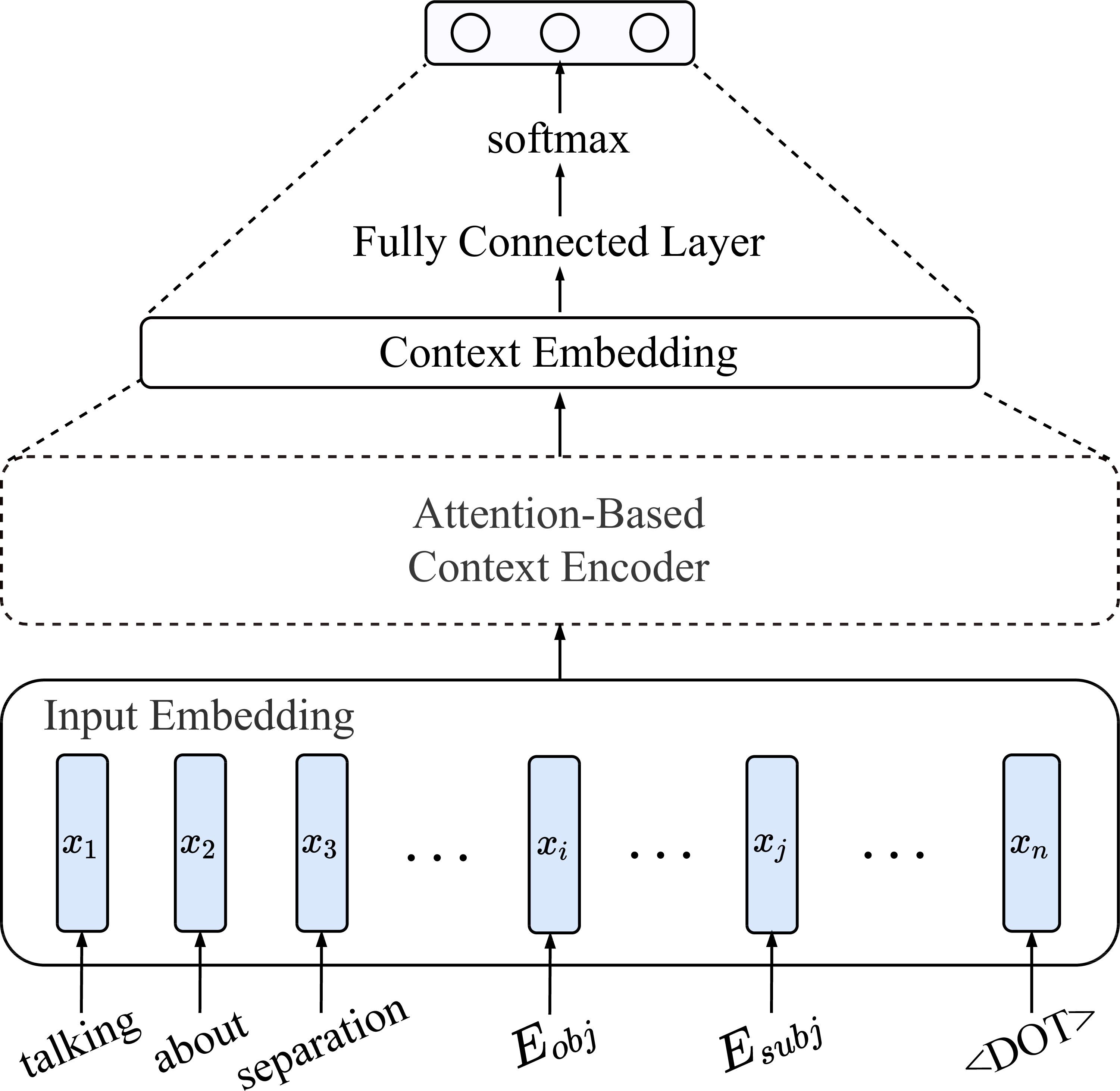
Figure 3. General, context-based 3-scale (positive, negative, neutral) classification model, with details on <<Attention-Based Context Encoder>> block in Section 5 and 6.

4. Model

In this paper, the problem of sentiment attitude extraction is treated as a classification task of two types: two-scale and three-scale. Given a pair of named entities, we predict a sentiment label of a pair, which could be as follows:

• sentiment, i.e. positive or negative (two-scale classification format);

• sentiment or neutral.

As the RuSentRel corpus provides opinions with positive or negative sentiment labels only (Section 3), we automatically added neutral sentiments for all pairs not mentioned in the annotation and co-occurred in the same sentences of the collection texts.

context

Говорить о разделении кавказского регионаwhiteкавказского региона из-за конфронтации РоссииwhiteРоссииobj и ТурцииwhiteТурцииsubj пока не приходится, хотя опасность есть.

Talking about the separation of the Caucasus regionwhiteCaucasus region due to the confrontation between RussiawhiteRussiaobj and TurkeywhiteTurkeysubj is not necessary, although there is a danger.

$\downarrow$

terms

Talking about the separation of the $\uline{\phantom{E}}\hbox to0.0pt{\hss\contour{white}{E}}$ due to the confrontationneg between $\uline{\phantom{E}}\hbox to0.0pt{\hss\contour{white}{E}}_{obj}$ and $\uline{\phantom{E}}\hbox to0.0pt{\hss\contour{white}{E}}_{subj}$ is not-necessaryneg <COMMA> although there is a danger <DOT>

Figure 4. An example of a context processing into a sequence of terms; attitude participants $\left<Russia,Turkey\right>$ and other mentioned entities become masked; frames are italic and optionally suffixed with the sentiment value of A0$\to$A1 polarity.

We consider a context as a text fragment that is limited by a single sentence and includes a pair of named entities. The general architecture is presented in Figure 3, where the sentiment could be extracted from the context. To present a context, we treat the original text as a sequence of terms $[t_{1},\ldots,t_{n{}}]$ limited by $n{}$, with the distance between attitude participants limited by $\eta{}$ terms. Each term belongs to one of the following groups: entities, frames, tokens, and words (if none of the prior has not been matched).

We use masked representation for attitude participants ($\uline{\phantom{E}}\hbox to0.0pt{\hss\contour{white}{E}}_{obj}$, $\uline{\phantom{E}}\hbox to0.0pt{\hss\contour{white}{E}}_{subj}$) and mentioned named entities ($\uline{\phantom{E}}\hbox to0.0pt{\hss\contour{white}{E}}$) to prevent models from capturing related information. To represent frames, we combine a frame entry with the corresponding A0$\to$A1 sentiment polarity value (and neutral if the latter is absent). We also invert sentiment polarity when an entry has "не" (not) preposition. The tokens group includes: punctuation marks, numbers, url-links. Each term of words is considered in a lemmatized form.

Figure 4 provides an example of a context processing into a sequence of input terms. All entries are encoded with the negative polarity A0$\to$A1: "конфронтация" (confrontation) has a negative polarity, and "не приходится" (not necessary) has a positive polarity of entry "necessary" which is inverted due to the "not" preposition.

To represent the context in a model, each term is embedded with a vector of fixed dimension. The sequence of embedded vectors $X{}=[x_{1},\ldots,x_{n{}}]$ is denoted as input embedding ($x_{i}\in\mathbb{R}^{m}{},i\in\overline{1..n{}}$). Sections 5 and 6 provide an encoder implementation in details. In particular, each encoder relies on input embedding and generates output embedded context vector $s{}$.

In order to determine a sentiment class by the embedded context $s{}$, we apply: (1) the hyperbolic tangent activation function towards $s{}$ and (2) transformation through the fully connected layer:

(1) $$r{}=W_{r}{}{}\cdot\tanh(s)+b_{r}{}{}$$

In Formula 1, $W_{r}{}{}\in\mathbb{R}^{|s{}|{}\times c{}}$ and $b_{r}{}{}\in\mathbb{R}^{c}{}$ correspond to the hidden states; $|s{}|{}$ correspond to the size of vector $s{}$, and $c{}\in\{2,3\}$ is a number of classes. Finally, the result $o=\sigma(r,c{})$ is an output vector of probabilities, which is computed by:

(2) $$\sigma(z,K{})_{i}{}=\frac{\exp(z_{i}{})}{\sum_{j=1}^{K{}}{\exp(z_{j})}}\hskip 28.45274ptz\in\mathbb{R}^{K{}}$$

5. Feature Attentive Context Encoders

In this section, we consider features as a significant for attitude identification context terms, towards which we would like to quantify the relevance of each term in the context. For a particular context, we select embedded values of the attitude participants ($\uline{\phantom{E}}\hbox to0.0pt{\hss\contour{white}{E}}_{obj}$, $\uline{\phantom{E}}\hbox to0.0pt{\hss\contour{white}{E}}_{subj}$).

Figure 5 illustrates a feature-based encoder  (Huang et al., 2016). In formulas 3–5, we describe the quantification process of a context embedding $X{}$ with respect to a particular feature $f\leavevmode\nobreak\ \in\leavevmode\nobreak\ F{}$. Given an $i$’th embedded term $x_{i}$, we concatenate its representation with $f$:

(3) $$h_{i}=\left[x_{i},f\right]$$

Figure 5. Feature-attentive context encoder architecture, based on AttCNN model (Huang et al., 2016).

The quantification of the relevance of $x_{i}$ with respect to $f$ is denoted as $u_{i}\leavevmode\nobreak\ \in\leavevmode\nobreak\ \mathbb{R}$ and calculated as follows:

(4) $$u_{i}=W_{a}\left(\tanh(W_{we}\cdot h_{i}+b_{we})\right)+b_{a}\hskip 14.22636pt$$

In Formula 4, $W_{we}\in\mathbb{R}^{2\cdot m\times\textbf{h}_{\textsc{mlp}}}$ and $W_{a}\in\mathbb{R}^{\textbf{h}_{\textsc{mlp}}{}}$ correspond to the weight and attention matrices respectively, and $\textbf{h}_{\textsc{mlp}}{}$ corresponds to the size of the hidden representation in the weight matrix. To deal with normalized weights within a context, we transform quantified values $u_{i}$ into probabilities $\alpha_{i}$ by Formula 2 as follows: $\alpha\leavevmode\nobreak\ =\leavevmode\nobreak\ \sigma(u,n{}$). We utilize Formula 5 to obtain attention-based context embedding $\hat{s}{}$ of a context with respect to feature $f$:

(5) $$\hat{s}{}=\sum_{i=1}^{n{}}x_{i}\cdot\alpha_{i}\hskip 28.45274pt\hat{s}{}\in\mathbb{R}^{m{}}$$

Applying Formula 5 towards each feature $f_{j}\in F{},\hskip 2.84544ptj\in\overline{1..k{}}$ results in vector $\{\hat{s}{}_{j}\}_{j=1}^{k{}}$. We use average-pooling to transform the latter sequence into single averaged vector $s_{f}{}\in\mathbb{R}^{m}{}$.

We also utilize a <<CNN encoder>> block (Figure 5) in order to compose the context representation $s_{cnn}{}$. The resulting context embedding vector $s{}$ is a concatenation of $s_{f}{}$ and $s_{cnn}{}$:

(6) $$s{}=[s_{f}{},s_{cnn}{}]$$

Structurally, a convolutional neural network based encoder is a sequence of the following transformations: convolutions and pooling. Figure 6 provides a detailed comparison between classic neural network (CNN, Figure 6(a)), and piecewise convolutional neural network (PCNN, Figure 6(b)).

Starting with the convolution operation, which remains equal across all the encoders of Figure 6, let $x_{a{}:b{}}$ is as consequent vectors concatenation from $a{}$’th till $b{}$’th positions. An application of ${\bf\omega}\in\mathbb{R}^{d},\hskip 2.84544pt(d=l{}\cdot m{})$ towards the concatenation $x_{a{}:b{}}$ is a sequence convolution by filter $\omega$, where $l{}$ is a filter window size, and $m{}$ corresponds to embedding vector size. For convolving calculation $c_{j{}}$ ($j{}\in\overline{1..n{}}{}$), we apply scalar multiplication as follows:

(7) $$c_{j{}}=\omega\cdot x_{j{}-l{}+1:j{}}$$

To get multiple feature combinations, a set of different filters $W\leavevmode\nobreak\ =\leavevmode\nobreak\ \{\omega_{1},\ldots,\omega_{t{}}\}{}$ has been applied towards $X{}$. This leads to a modified version of Formula 7 by introduced layer index $i{}$:

(8) $$c_{i{},j{}}=\omega_{i{}}\cdot x_{j{}-l{}+1:j{}}$$

Denoting ${\bf c}_{i}=\{c_{i,1},\ldots,c_{i,n}\}$ in Formula 8 we reduce the latter by index $j{}\in\overline{1..n{}}{}$ and compose a matrix $C{}\leavevmode\nobreak\ =\leavevmode\nobreak\ \{{\bf c}_{1},{\bf c}_{2},\ldots,{\bf c}_{t}\}{}$ which represents convolution matrix with shape $C{}\leavevmode\nobreak\ \in\leavevmode\nobreak\ \mathbb{R}^{n{}\times t{}}$.

Max-pooling is an operation that reduces values by keeping maximum. In original CNN architecture (Figure 6(a)), max pooling applies separately per each convolution layers ${\bf c}_{i{}}$, which results in ${\bf p}\leavevmode\nobreak\ \in\leavevmode\nobreak\ \mathbb{R}^{t{}}$. It reduces convolved information quite rapidly which is not appropriate for attitude classification task. To keep context features that are inside and outside of the attitude entities, authors (Zeng et al., 2015) perform piecewise max-pooling (Figure 6(b)). Given attitude entities as borders, we divide each ${\bf c}_{i{}}$ into inner, left and right segments $\{{\bf c}_{i{},1},{\bf c}_{i{},2},{\bf c}_{i{},3}\}$. Then max-pooling applies per each segment separately:

(9) $$p_{i{},q{}}=\max({\bf c}_{i{},q{}}),\hskip 5.69046pti{}\in\overline{1..t{}}{},\hskip 5.69046ptq{}\in\{1,2,3\}$$

Thus, for each ${\bf c}_{i{}}$ we have a set ${\bf p}_{i{}}\leavevmode\nobreak\ =\leavevmode\nobreak\ \{p_{i{},1},p_{i{},2},p_{i{},3}\}{}$. Concatenation of these sets for each layer $i{}$ results in ${\bf p}\in\mathbb{R}^{3t{}}$ and that is a result of piecewise max-pooling operation.

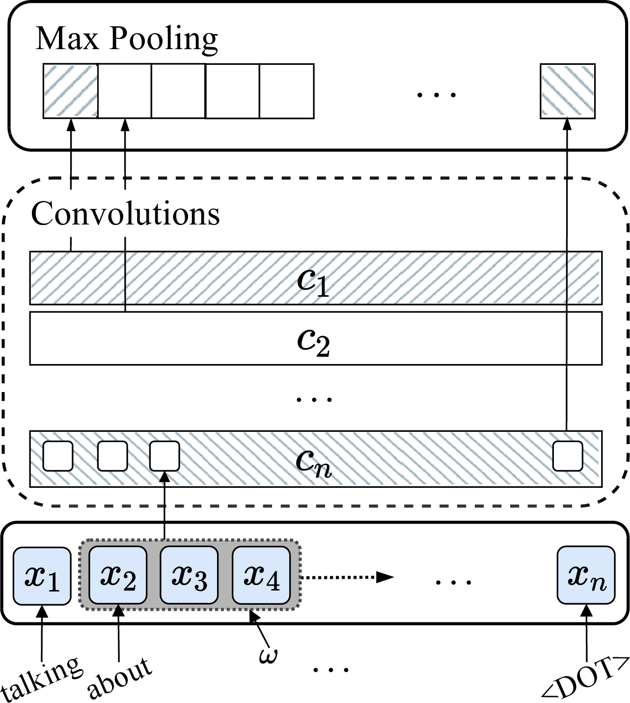
(a) CNN

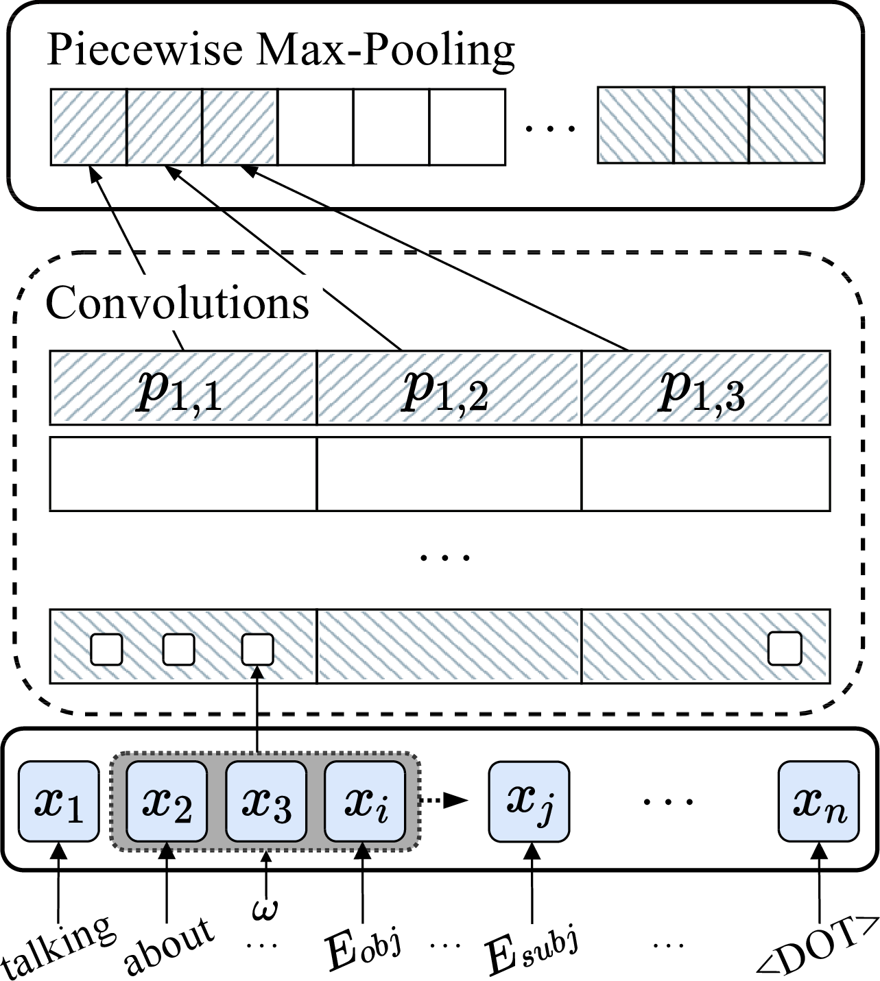
(b) PCNN (Zeng et al., 2015)

Figure 6. Comparison of CNN-based context encoders; $\omega$ corresponds to convolutional filter window, size of 3.

6. Self Attentive Context Encoders

In section 5 the application of attention in context embedding fully relies on the sequence of predefined features. The quantification of context terms is performed towards each feature. In turn, the self-attentive approach assumes to quantify a context with respect to an abstract parameter. Unlike quantification methods in feature-attentive embedding models, here the latter is replaced with a hidden state ($w$) which modified during the training process.

To learn the hidden term semantics for each input, we utilize the LSTM (Hochreiter and Schmidhuber, 1997) recurrent neural network architecture, which addresses learning long-term dependencies by avoiding gradient vanishing and expansion problems. The calculation $h_{t}$ of $t$’th embedded term $x_{t}$ is based on prior state $h_{t-1}$, where the latter acts as a parameter of auxiliary functions (Hochreiter and Schmidhuber, 1997). Figure 7 illustrates the attention-based sentence encoder architecture, builded on top of the BiLSTM – is a bi-directional LSTM to obtain a pair of sequences $\overrightarrow{h}$ and $\overleftarrow{h}$   ($\overrightarrow{h_{i}},\overleftarrow{h_{i}}\in\mathbb{R}^{\textbf{h}{}}$). The resulting context representation $H=[h_{1},\leavevmode\nobreak\ \ldots,\leavevmode\nobreak\ h_{n{}}]$ is composed as the concatenation of bi-directional sequences elementwise: $h_{i}=\overrightarrow{h_{i}}+\overleftarrow{h_{i}},\hskip 2.84544pti\in\overline{1..n{}}$. The quantification of hidden term representation $h_{i}\in\mathbb{R}^{2\cdot\textbf{h}{}}$ with respect to $w\in\mathbb{R}^{2\cdot\textbf{h}{}}$ is described in formulas 10-11.

(10) $$m_{i}=\tanh(h_{i})$$

(11) $$u_{i}=m_{i}^{T}\cdot w$$

Figure 7. Self-attentive context encoder architecture, with self-attention module of Att-BLSTM model (Zhou et al., 2016) over bi-directional LSTM encoder.

In order to deal with normalized weights, we transoform quantified values $u_{i}$ into $\alpha_{i}$ as follows: $\alpha=\sigma(u,n{})$ (Formula 2). The resulting context embedding vector $s{}$ is an activated weighted sum of each parameter of context hidden states:

(12) $$s{}=tanh(H\cdot\alpha)\hskip 28.45274pts{}\in\mathbb{R}^{2\cdot\textbf{h}{}}$$

7. Model Details

		Two-scale					Three-scale
Model	DS	$F1_{avg}$	$F1_{cv}^{1}$	$F1_{cv}^{2}$	$F1_{cv}^{3}$	$F1_{\textsc{test}{}}$	$F1_{avg}$	$F1_{cv}^{1}$	$F1_{cv}^{2}$	$F1_{cv}^{3}$	$F1_{\textsc{test}{}}$
Att-BLSTM	$\bullet$	0.667	0.71	0.62	0.67	0.68	0.332	0.36	0.33	0.31	0.38
BiLSTM	$\bullet$	0.653	0.70	0.60	0.66	0.70	0.312	0.34	0.31	0.29	0.39
Att-BLSTM		0.640	0.69	0.60	0.64	0.68	0.314	0.35	0.27	0.32	0.32
BiLSTM		0.632	0.66	0.63	0.61	0.67	0.286	0.32	0.26	0.28	0.34
AttPCNNe	$\bullet$	0.644	0.67	0.61	0.65	0.66	0.312	0.33	0.30	0.31	0.41
PCNN	$\bullet$	0.599	0.70	0.53	0.57	0.63	0.315	0.33	0.30	0.31	0.40
AttPCNNe		0.617	0.64	0.56	0.65	0.67	0.297	0.32	0.29	0.28	0.35
PCNN		0.608	0.62	0.58	0.63	0.66	0.285	0.29	0.27	0.30	0.32
AttCNNe	$\bullet$	0.631	0.64	0.64	0.62	0.66	0.316	0.35	0.29	0.30	0.41
CNN	$\bullet$	0.625	0.62	0.63	0.63	0.68	0.305	0.31	0.30	0.31	0.40
AttCNNe		0.636	0.66	0.64	0.61	0.62	0.270	0.33	0.23	0.25	0.30
CNN		0.553	0.60	0.56	0.51	0.59	0.274	0.30	0.26	0.26	0.31

Table 2. Experiment (Two-scale and Three-scale) context classification results by $F1$ measure over RuSentRel collection; all the models are separated into the following groups (from top to bottom): BiLSTM, PCNN, CNN; models that employ RuAttitudes in the training process (DS mode) are labeled with <<$\bullet$>>; columns related to result evaluation in each experiment (from left to right): (1) average value in CV-3 experiment ($F1_{avg}$) with results on each split ($F1_{cv}^{i},\hskip 2.84544pti\in\overline{1..3}$), (2) results on train/test separation ($F1_{\textsc{test}{}}{}$).

We provide embedding details of context term groups described in Section 4. For words and frames, we look up for vectors in precomputed and publicly available model $M_{word}$ based on news articles with window size of $20{}$, and vector size of $1000{}$. Each term that is not presented in model we treat as a sequence of parts ($n$-grams) and look up for related vectors in $M_{word}$ to complete an averaged vector. For a particular part, we start with trigrams ($n=3$) and decrease $n$ until the related $n$-gram is found. For masked entities ($\uline{\phantom{E}}\hbox to0.0pt{\hss\contour{white}{E}}$, $\uline{\phantom{E}}\hbox to0.0pt{\hss\contour{white}{E}}_{obj}$, $\uline{\phantom{E}}\hbox to0.0pt{\hss\contour{white}{E}}_{subj}$) and  tokens, each element embedded with a vector of size 1000; every vector is randomly initialized from a Gaussian distribution (Glorot and Bengio, 2010).

Each context term has been additionally expanded with the following parameters:

• Distance embedding (Rusnachenko and Loukachevitch, 2018) ($v_{\textsc{d}\mathchar 45\relax obj}$, $v_{\textsc{d}\mathchar 45\relax subj}$) – is vectorized distance in terms from attitude participants of entry pair ($\uline{\phantom{E}}\hbox to0.0pt{\hss\contour{white}{E}}_{obj}$ and $\uline{\phantom{E}}\hbox to0.0pt{\hss\contour{white}{E}}_{subj}$ respectively) to a given term;

• Closest to synonym distance embedding ($v_{\textsc{sd}\mathchar 45\relax obj}$, $v_{\textsc{sd}\mathchar 45\relax subj}$) is a vectorized absolute distance in terms from a given term towards the nearest entity, synonymous to $\uline{\phantom{E}}\hbox to0.0pt{\hss\contour{white}{E}}_{obj}$ and $\uline{\phantom{E}}\hbox to0.0pt{\hss\contour{white}{E}}_{subj}$;

• Part-of-speech embedding ($v_{\textsc{pos}}$) is a vectorized tag for words (for terms of other groups considering <<unknown>> tag);

• A0$\to$A1 polarity embedding ($v_{A0\to A1}$) is a vectorized <<positive>> or <<negative>> value for frame entries whose description in RuSentiFrames provides the corresponding polarity (otherwise considering <<neutral>> value); polarity is inverted when an entry has "не" (not) preposition.

7.1. Training

This process assumes hidden parameter optimization of a given model. We utilize an algorithm described in (Rusnachenko and Loukachevitch, 2018). The input is organized in minibatches, where each minibatch yields of $l{}$ bags. Each bag has a set of $t{}$ pairs $\left<X{}_{j},y_{j}\right>_{j=1}^{t{}}$, where each pair is described by an input embedding $X{}_{j}$ with the related label $y_{j}\in\mathbb{R}^{c}{}$. The training process is iterative, and each iteration includes the following steps in order to calculate vector $cost$ and perform hidden states update.

The first step assumes a minibatch composing, which is consist of $l{}$ bags of size $t{}$. Then we perform a forward propagation through the network which results in a vector (size of $q=l{}\cdot t{}$) of outputs $o_{k}\in\mathbb{R}^{c}{}$. In the third step we calculate cross entropy loss for an output vector as follows:

(13) $$L_{k}=\sum\limits_{j=1}^{c}{}\log p(y_{i}|o_{k,j};\theta),\hskip 2.84544ptk\in\overline{1..q}$$

In the final step we compose a $cost$ vector, where $i$’th component $cost_{i}$ ($i=\overline{1..l{}}$) corresponds to the maximal cross entropy loss within a related $i$’th bag:

(14) $$cost_{i}=\max\left[L_{(i-1)\cdot t}\hskip 2.84544pt..\hskip 2.84544ptL_{i\cdot t}\right)$$

7.2. Parameters settings

The minibatch size ($l{}$) is set to $2$, where contexts count per bag $t{}$ is set to $3$. All the contexts were limited by $n{}=50{}$ terms, with the distance between attitude participants limited to $\eta{}=10{}$ terms. For embedding parameters (Section 2) we use vectors with size of $5{}$. For CNN and PCNN context encoders, the size of convolutional window ($\omega$) and filters count (c) were set to $3$ and $300$ respectively. As for parameters related to sizes of hidden states in Sections 5 and 6: $\textbf{h}_{\textsc{mlp}}{}=10$, $\textbf{h}{}=128{}$. We utilize the AdaDelta optimizer with parameters $\rho=0.95$ and $\epsilon=10^{-6}$ (Zeiler, 2012). To prevent models from overfitting, we apply $dropout$ towards the output with keep probability set to $0.8$. For hidden state values initialization we utilize Xavier weight intializer (Glorot and Bengio, 2010).

8. Experiments

According to Section 4, we treat sentiment attitude extraction as a classification task of different scales of output classes. We train and evaluate all the models in the following experiments:

1. Two-scale (Rusnachenko et al., 2019), in which all the models have to predict a sentiment label of an attitude in context. It is important to note that for each document we consider only those attitudes that might be fitted in a context;

2. Three-scale (Rusnachenko and Loukachevitch, 2018), in which each model might classify a given context with an attitude in it as sentiment-oriented (positive/negative) or neutral.

It is worth to note that the evaluation process in case of Two-scale experiment assumes to treat only those pairs in comparison, which could be found within a context of the related document.

8.1. Datasets and Evaluation formats

The evaluation in experiments has been performed over the RuSentRel corpus, using the following formats:

1. CV-based format, in which it is supposed to utilize 3-fold cross-validation (CV); all folds are equal in terms of sentence count;

2. Fixed format, in which the predefined separation of documents onto train/test sets is considered.

For evaluating models in this task, we adopt macro-averaged F1-score ($F1$) over documents. F1-score is considered averaging of the positive and negative classes, which are most important in attitude analysis.

8.2. Model Comparisons and Training

In terms of architecture aspects, all the models differ only in sentence encoder implementation of a single context classification model (Figure 3). The list of the models selected for the experiments is as follows:

• CNN model with a classic convolutional neural network architecture (Figure 6(a));

• PCNN model, in which the encoder treats each convolution layer in parts, relatively to the attitude participants’ positions in the context (Figure 6(b));

• AttCNN_e, AttPCNN_e are models with feature attentive encoders (Section 5); <<e>> corresponds to the set of attitude participants ($\uline{\phantom{E}}\hbox to0.0pt{\hss\contour{white}{E}}_{obj}$, $\uline{\phantom{E}}\hbox to0.0pt{\hss\contour{white}{E}}_{subj}$).

• BiLSTM is a bi-directional LSTM (Hochreiter and Schmidhuber, 1997);

• Att-BLSTM model (Section 6);

For a particular model, the training (and related evaluation) process has been performed in the following modes:

1. DS, is an application of distant supervision, which is considered as a combination of RuSentRel and RuAttitudes collections;

2. SL, is supervised learning, using RuSentRel.

It is worth to clarify the details of the training set creation in DS mode depending on the evaluation formats (Section 8.1):

• For CV-based, in each split, the RuAttitudes collection is combined with each training block of the RuSentRel collection;

• For Fixed, the training set represents a combination of RuAttitudes with the train part.

We measure $F1$ on the training part every 10 epoch. The number of epochs was limited by 150. The training process terminates when $F1$ on the training part becomes greater than $0.85$.

8.3. Result Analysis

Table 2 provides the results in the experiments for models organized (and separated) into the following groups: CNN, PCNN, BiLSTM. To access the effectiveness of both an application of distant supervision in the training process (DS mode, marked with <<$\bullet$>> sign in Table 2) and attention-based encoders (prefixed with <<Att>>), we provide efficiency assessment in the following directions:

1. Application of DS mode for baselines;

2. Application of attention-based sentence encoders in DS mode.

		Two-scale			Three-scale
Ratio	Parameter	CNN	PCNN	BiLSTM	CNN	PCNN	BiLSTM
$E_{DS}$	$F1_{avg}$	0.13	$\cdot$	0.01	0.11	0.11	0.09
	$F1_{\textsc{test}{}}{}$	0.15	$\cdot$	0.04	0.29	0.25	0.15
$E_{DSA}$	$F1_{avg}$	0.01	0.08	0.02	0.04	$\cdot$	0.06
	$F1_{\textsc{test}{}}{}$	$\cdot$	0.05	$\cdot$	0.03	0.03	$\cdot$

Table 3. Calculated $E_{DS}$ and $E_{DSA}$ ratios in each experiment for CV-based ($F1_{avg}$) and Fixed ($F1_{\textsc{test}{}}{}$) evaluation formats; values below zero displayed as <<$\cdot$>>

To accomplish the comparison in a particular experiment, for each model we calculate the corresponding ratios by $F1_{avg}$ and $F1_{\textsc{test}{}}{}$:

• $E_{DS}$ – is the effectiveness of baseline models trained in DS mode over a related baseline that trained in SL mode;

• $E_{DSA}$ – is the effectiveness of models trained in DS mode with attention-based sentence encoder (prefixed with Att) over related baseline version.

Table 3 provides calculated ratios for the Two-scale and Three-scale experiments. The ratio calculation ($r$) for a result $A$ over a result $B$ performed as follows: $r=A/B-1$.

Analyzing results in the Two-scale experiment by $E_{DS}$ in Table 3, model AttCNN_e shows a significant increase in 13% and 15% in case of CV-based and Fixed evaluation formats respectively. An application of attention-based encoders does not illustrate an increase in result model quality, only 1% for AttCNN_e and 5-8% for AttPCNN_e. The highest result is obtained by the Att-BLSTM model with a 4% increase by $E_{DS}$.

As for the Three-scale experiment, it is also possible to investigate a significant increase by $E_{DS}$ with 10% in the CV-based evaluation mode and 15-29% on the test part (Fixed evaluation format). Utilizing attentive encoders in the models that employ RuAttitudes in training provides 3% results improvement according to $E_{DSA}$ ratio. The highest increase by $E_{DSA}$ is achieved by Att-BLSTM model with 6% when the model is evaluated in the CV-based format.

9. Analysis of Attention Weights

According to Section 3.3, one of the assumptions behind the distant supervision application for RuAttitudes collection developing is that the attitude might be conveyed by a frame of a certain sentiment polarity. For models of the Three-scale experiment with attention-based encoders (AttCNN_e, AttPCNN_e, Att-BLSTM), in this section, we analyze how contexts with sentiment and neutral attitudes affect on weight distribution in dependence on the term type.

Att-BLSTM (DS)
frames	nouns	prep	sentiment
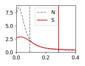
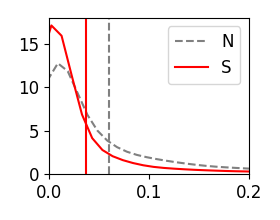
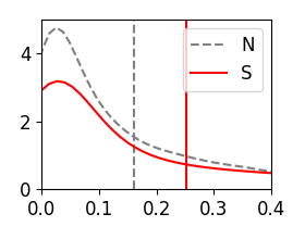
Att-BLSTM (SL)
frames	nouns	prep	sentiment
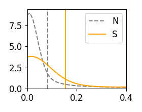
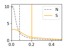
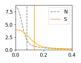
AttCNNe (DS)
frames	nouns	prep	sentiment
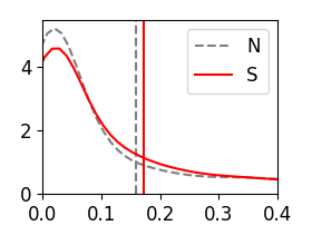
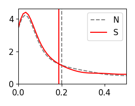
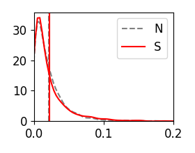
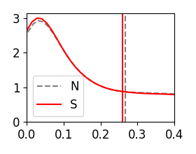
AttCNNe (SL)
frames	nouns	prep	sentiment

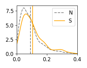
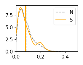
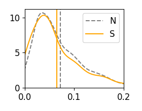
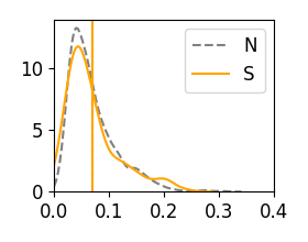
Figure 8. Kernel density estimations (KDE) of context-level weight distributions across neutral (N) and sentiment (S) context sets for models Att-BLSTM and AttCNN_e trained in different modes: distant supervision application (DS), and supervised learning only (SL); the probability range (x-axis) scale depends on the group of terms: $[0,0.4]$ (frames, sentiment), $[0,0.5]$ (nouns), and $[0,0.2]$ (prep); vertical lines indicate expected values of corresponding distributions.

Model	DS	$D_{F}$	$D_{N}$	$D_{P}$	$D_{S}$	$D_{V}$
Att-BLSTM	$\bullet$	0.29	0.23	0.26	0.14	0.17
Att-BLSTM		0.13	0.22	0.08	0.11	0.07
AttCNNe	$\bullet$	0.05	0.03	0.05	0.03	0.03
AttCNNe		0.09	0.07	0.09	0.07	0.07
AttPCNNe	$\bullet$	0.10	0.03	0.04	0.04	0.06
AttPCNNe		0.09	0.17	0.15	0.08	0.06

Table 4. Calculated statistics ($D_{*}$) from Kolmogorov-Smirnov test by following term groups: frames (F), nouns (N), prep (P), sentiment (S), and verbs (V); highest and second highest values per each category are bolded and underlined respectively.

Model	DS	$\Delta_{F}$	$\Delta_{N}$	$\Delta_{P}$	$\Delta_{S}$	$\Delta_{V}$
Att-BLSTM	$\bullet$	0.20	-0.09	-0.02	0.09	$\cdot$
Att-BLSTM		0.07	0.12	0.03	0.05	0.03
AttCNNe	$\bullet$	$\cdot$	$\cdot$	$\cdot$	$\cdot$	$\cdot$
AttCNNe		$\cdot$	$\cdot$	$\cdot$	$\cdot$	$\cdot$
AttPCNNe	$\bullet$	0.06	$\cdot$	$\cdot$	$\cdot$	$\cdot$
AttPCNNe		$\cdot$	-0.02	$\cdot$	$\cdot$	$\cdot$

Table 5. The difference in estimated values of $\rho_{\textsc{s}}$ and $\rho_{\textsc{n}}$ ($\Delta_{*{}}$) by following term groups: frames (F), nouns (N), prep (P), sentiment (S), and verbs (V); absolute max values by each term group are bolded; absolute values less or equal $0.1$ displayed as <<$\cdot$>>

Att-BLSTM (SL) (Original)

…

…

Att-BLSTM (SL)

…

…

Att-BLSTM (DS)

…

…

Figure 9. Weight distribution visualization on sentiment contexts for model Att-BLSTM, trained in different modes: supervised learning (SL), and with an application of distant supervision (DS); for visualization purposes, weight of each term is normalized by the maximum in context; frame entries (marked italic and bolded) appeared between masked attitude participants become greater weighted when training process employs RuAttitudes (DS mode).

The terms quantification process remains a significant part of each attention-based encoder. Being assigned and normalized, weights of every term in a context might be treated as probability weight distribution across all the terms appeared in a context.

The source of documents for contexts in this analysis is the test part of the RuSentRel collection (Section 8.1). We analyse the weight distribution of the frames group, declared in Section 4, across all input contexts. We additionally introduce a list of extra groups utilized in the analysis by separating the subset of words into prepositions (prep), terms appeared in RuSentiLex lexicon (sentiment, Section 3), nouns (nouns), and verbs (verbs). The contents of nouns and verbs is considered only for those entries that are not present in the RuSentiLex lexicon.

The context-level weight of a particular term group is a weighted sum of terms which both appear in the context and belong to the corresponding term group. For discrepancy analysis between sentiment and neutrally labeled contexts, we utilize distributions of context-levels weights across:

1. Sentiment contexts (S) – contexts, labeled with positive or negative labels;

2. Neutral contexts (N) – contexts, labeled as neutral.

Further, such weight distributions over sentiment and neutral contexts denoted as $\rho_{\textsc{s}}^{*{}}$ and $\rho_{\textsc{n}}^{*{}}$ respectively, where asterisk corresponds to the certain term group.

To reveal the difference between distributions, the statistics from Kolmogorov-Smirnov test was used (Massey Jr, 1951). In our analysis, the calculation of such statistics is considered to be performed between a pair of samples (tabulated distributions), where each sample is a sequence of term group probabilities within each context. It is worth to note that such tabulated distributions meet the criteria of the independence of values (weights) related to continious set. Considering the latter, we are able to switch from tabulated to the cumulative distributions as follows:

(15) $$\mathrm{F}^{*{}}_{\mathrm{X}}(x)=\mathrm{P}(\mathrm{X}<x)=\int_{-\infty}^{x}\rho^{*{}}_{\mathrm{X}}(t)dt$$

where $\mathrm{X}$ is related to the contexts set of a certain polarity (sentiment or neutral), i.e. $\mathrm{X}\in\{\textsc{S},\textsc{N}\},x\in[0,1]$. The Kolmogorov-Smirnov statistics (KS-statistics) represent the maximum of the absolute deviation between cumulative distributions $\mathrm{F}^{*{}}_{\textsc{S}}$ and $\mathrm{F}^{*{}}_{\textsc{N}}$:

(16) $$D_{*{}}=\sup_{x\in[0,1]}|\mathrm{F}^{*{}}_{\textsc{S}}(x)-\mathrm{F}^{*{}}_{\textsc{N}}(x)|$$

Table 4 provides the calculated KS-statistics (Formula 16) separately for each group of terms. Larger values by $D_{*{}}$ address on a greater difference in weights distribution between $\rho_{\textsc{s}}^{*{}}$ and $\rho_{\textsc{n}}^{*{}}$.

Another statistics that we utilize in analysis is a difference in estimated values of $\rho_{\textsc{s}}^{*{}}$ and $\rho_{\textsc{n}}^{*{}}$:

(17) $$\Delta_{*{}}=E(\rho_{\textsc{s}}^{*{}})-E(\rho_{\textsc{n}}^{*{}})$$

In addition to KS-statistics, the calculation of $\Delta_{*{}}$ provides the sign of the difference. Summarizing results of both statistics, we may conclude that among all the models presented in our analysis, only Att-BLSTM illustrates a significant difference between $\rho_{\textsc{n}}$ and $\rho_{\textsc{s}}$ across all the term groups. The comparative kernel density estimations of context weight distributions for Att-BLSTM and AttCNN_e is presented in Figure 8. In case of Att-BLSTM, application of RuAttitudes in training (DS mode) results in weights distribution biasing from nouns and prep onto terms of the frames and sentiment groups in sentiment contexts. The similar case is observed for AttCNN_e trained in DS mode: terms of frames and sentiment groups become more valuable equally in sentiment and neutral context sets. The assumption here is a structure of contexts in RuAttitudes (Section 3.3): all the contexts enriched with frames, appeared between attitude participants. Those cases where frames convey the presence of an attitude in context are presented in Figure 9. According to the provided examples for Att-BLSTM model, it is possible to investigate greater weighted frame entries when the training process of related model employs RuAttitudes.

Overall, the model Att-BLSTM stands out baselines and models with feature-based attention encoders (AttCNN_e, AttPCNN_e) both due to results (Section 8) and the greatest discrepancy between $\rho_{\textsc{s}}$ and $\rho_{\textsc{n}}$ across all the term groups presented in the analysis (Figure 8). We assume that the latter is achieved due to the following factors: (1) application of bi-directional LSTM encoder; (2) utilization of a single trainable vector ($w$) in the quantification process (Section 6) while the models of feature-based approach (Section 5, Formula 4) depend on fully-connected layers.

Conclusion

In this paper, we study the attention-based models, aimed to extract sentiment attitudes from analytical articles. We consider the problem of extraction as two-class and three-class classification tasks for whole documents. Depending on the task, the described models should classify a context with an attitude mentioned in it onto the following classes: positive or negative (two-class); positive, negative, or neutral (three-class).

We investigated two types of attention embedding approaches: (1) feature-based, (2) self-based. To fine-tune the attention mechanism, we utilized distant supervision technique by employing RuAttitudes collection in the training process.

We conducted experiments on Russian analytical texts of the RuSentRel corpus and provided analysis of the results. The affection of distant-supervision technique onto attention-based encoders was shown by the variety in weight distribution of certain term groups between sentiment and non-sentiment contexts. Utilizing the distant-supervision approach in training three-class classification models results in 10% improvement by $F1$ for architectures that do not employ attention module in context encoder. Replacing the latter with attention-based encoders provides the classification improvement by 3% $F1$.

In further work we plan to study application of language models for the presented tasks, as it continues the idea of attentive encoders application.

Acknowledgments

The reported study was funded by RFBR according to the research project № 20-07-01059.

References

- (1)
- Arkhipenko et al. (2016) K Arkhipenko, I Kozlov, J Trofimovich, K Skorniakov, A Gomzin, and D Turdakov. 2016. Comparison of neural network architectures for sentiment analysis of russian tweets. In Proceedings of international conference, computational linguistics and intellectual technologies.
- Cho et al. (2014) Kyunghyun Cho, Bart van Merriënboer, Caglar Gulcehre, Dzmitry Bahdanau, Fethi Bougares, Holger Schwenk, and Yoshua Bengio. 2014. Learning Phrase Representations using RNN Encoder–Decoder for Statistical Machine Translation. In Proceedings of the 2014 Conference on Empirical Methods in Natural Language Processing (EMNLP). 1724–1734.
- Dowty (1991) David Dowty. 1991. Thematic proto-roles and argument selection. language 67, 3 (1991), 547–619.
- Glorot and Bengio (2010) Xavier Glorot and Yoshua Bengio. 2010. Understanding the difficulty of training deep feedforward neural networks. In Proceedings of the thirteenth international conference on artificial intelligence and statistics. 249–256.
- Hendrickx et al. (2009) Iris Hendrickx, Su Nam Kim, Zornitsa Kozareva, Preslav Nakov, Diarmuid Ó Séaghdha, Sebastian Padó, Marco Pennacchiotti, Lorenza Romano, and Stan Szpakowicz. 2009. Semeval-2010 task 8: Multi-way classification of semantic relations between pairs of nominals. In Proceedings of the Workshop on Semantic Evaluations: Recent Achievements and Future Directions. 94–99.
- Hochreiter and Schmidhuber (1997) Sepp Hochreiter and Jürgen Schmidhuber. 1997. Long short-term memory. Neural computation 9, 8 (1997), 1735–1780.
- Huang et al. (2016) Xuanjing Huang et al. 2016. Attention-based convolutional neural network for semantic relation extraction. In Proceedings of COLING 2016, the 26th International Conference on Computational Linguistics: Technical Papers. 2526–2536.
- Kuratov and Arkhipov (2019) Yuri Kuratov and Mikhail Arkhipov. 2019. Adaptation of deep bidirectional multilingual transformers for russian language. arXiv preprint arXiv:1905.07213 (2019).
- Loukachevitch and Levchik (2016) Natalia Loukachevitch and Anatolii Levchik. 2016. Creating a general russian sentiment lexicon. In Proceedings of the Tenth International Conference on Language Resources and Evaluation (LREC’16). 1171–1176.
- Loukachevitch and Rusnachenko (2018) Natalia Loukachevitch and Nicolay Rusnachenko. 2018. Extracting sentiment attitudes from analytical texts. Proceedings of International Conference on Computational Linguistics and Intellectual Technologies Dialogue-2018 (arXiv:1808.08932) (2018), 459–468.
- Massey Jr (1951) Frank J Massey Jr. 1951. The Kolmogorov-Smirnov test for goodness of fit. Journal of the American statistical Association 46, 253 (1951), 68–78.
- Mintz et al. (2009) Mike Mintz, Steven Bills, Rion Snow, and Dan Jurafsky. 2009. Distant supervision for relation extraction without labeled data. In Proceedings of the Joint Conference of the 47th Annual Meeting of the ACL and the 4th International Joint Conference on Natural Language Processing of the AFNLP: Volume 2-Volume 2. Association for Computational Linguistics, 1003–1011.
- Rogers et al. (2018) Anna Rogers, Alexey Romanov, Anna Rumshisky, Svitlana Volkova, Mikhail Gronas, and Alex Gribov. 2018. Rusentiment: An enriched sentiment analysis dataset for social media in russian. In Proceedings of the 27th International Conference on Computational Linguistics. 755–763.
- Rusnachenko and Loukachevitch (2018) Nicolay Rusnachenko and Natalia Loukachevitch. 2018. Neural Network Approach for Extracting Aggregated Opinions from Analytical Articles. In International Conference on Data Analytics and Management in Data Intensive Domains. Springer, 167–179.
- Rusnachenko et al. (2019) Nicolay Rusnachenko, Natalia Loukachevitch, and Elena Tutubalina. 2019. Distant Supervision for Sentiment Attitude Extraction. Proceedings of the International Conference on Recent Advances in Natural Language Processing (RANLP 2019) (2019).
- Shen and Huang (2016) Yatian Shen and Xuanjing Huang. 2016. Attention-Based Convolutional Neural Network for Semantic Relation Extraction. In Proceedings of COLING 2016, the 26th International Conference on Computational Linguistics: Technical Papers. 2526–2536.
- Tutubalina et al. (2020) Elena Tutubalina, Ilseyar Alimova, Zulfat Miftahutdinov, Andrey Sakhovskiy, Valentin Malykh, and Sergey Nikolenko. 2020. The Russian Drug Reaction Corpus and Neural Models for Drug Reactions and Effectiveness Detection in User Reviews. arXiv preprint arXiv:2004.03659 (2020).
- Yang et al. (2016) Zichao Yang, Diyi Yang, Chris Dyer, Xiaodong He, Alex Smola, and Eduard Hovy. 2016. Hierarchical attention networks for document classification. In Proceedings of the 2016 conference of the North American chapter of the association for computational linguistics: human language technologies. 1480–1489.
- Zeiler (2012) Matthew D Zeiler. 2012. ADADELTA: an adaptive learning rate method. arXiv preprint:1212.5701 (2012).
- Zeng et al. (2015) Daojian Zeng, Kang Liu, Yubo Chen, and Jun Zhao. 2015. Distant supervision for relation extraction via piecewise convolutional neural networks. In Proceedings of the 2015 Conference on Empirical Methods in Natural Language Processing. 1753–1762.
- Zhou et al. (2016) Peng Zhou, Wei Shi, Jun Tian, Zhenyu Qi, Bingchen Li, Hongwei Hao, and Bo Xu. 2016. Attention-based bidirectional long short-term memory networks for relation classification. In Proceedings of the 54th annual meeting of the association for computational linguistics (volume 2: Short papers). 207–212.