Inference in Stochastic Epidemic Models via Multinomial Approximations

Abstract

We introduce a new method for inference in stochastic epidemic models which uses recursive multinomial approximations to integrate over unobserved variables and thus circumvent likelihood intractability. The method is applicable to a class of discrete-time, finite-population compartmental models with partial, randomly under-reported or missing count observations. In contrast to state-of-the-art alternatives such as Approximate Bayesian Computation techniques, no forward simulation of the model is required and there are no tuning parameters. Evaluating the approximate marginal likelihood of model parameters is achieved through a computationally simple filtering recursion. The accuracy of the approximation is demonstrated through analysis of real and simulated data using a model of the 1995 Ebola outbreak in the Democratic Republic of Congo. We show how the method can be embedded within a Sequential Monte Carlo approach to estimating the time-varying reproduction number of COVID-19 in Wuhan, China, recently published by Kucharski et al. (2020).

1 Introduction

Compartmental models are used for predicting the scale and duration of epidemics, estimating epidemiological parameters such as reproduction numbers, and guiding outbreak control measures (Brauer, 2008; O’Neill, 2010; Kucharski et al., 2020). They are increasingly important because they allow joint modelling of disease dynamics and multimodal data, such as medical test results, cell phone and transport flow data (Rubrichi et al., 2018; Wu et al., 2020), census and demographic information (Prem et al., 2020). However, statistical inference in stochastic variants of compartmental models is a major computational challenge (Bretó, 2018). The likelihood function for model parameters is usually intractable because it involves summation over a prohibitively large number of configurations of latent variables representing counts of subpopulations in disease states which cannot be observed directly.

This has lead to the recent development of sophisticated computational methods for approximate inference involving various forms of stochastic simulation (Funk and King, 2020). Examples include Approximate Bayesian Computation (ABC) (Kypraios et al., 2017; McKinley et al., 2018; Brown et al., 2018, 2016), Data Augmentation Markov Chain Monte Carlo (MCMC) (Lekone and Finkenstädt, 2006), Particle Filters (Murray et al., 2018), Iterated Filtering (Stocks, 2019), and Synthetic Likelihood (Fasiolo et al., 2016). These methods continue to have real public health impact, for example the ABSEIR R package of Brown et al. (2018) features in the current UK COVID-19 surveillance protocols (de Lusignan et al., 2020). However the intricacy of these methods, their substantial computational cost arising from use of stochastic simulation, and their dependence on tuning parameters are obstacles to their wider use and scalability. The present work addresses the challenge of finding alternative inference techniques which are computationally simple and easy to use.

Contributions

We introduce a new approach to inference in compartmental epidemic models which:

• applies to a class of finite population, partially observed, discrete-time, stochastic models. In contrast to ODE models, these models can account for statistical variability in disease dynamics;

• allows approximate evaluation of the likelihood function for model parameters, and filtering and smoothing for compartment occupation numbers, without any stochastic simulation or algorithm tuning parameters, in contrast to state-of-the-art techniques such as ABC;

• revolves around a computationally simple filtering recursion. The resulting likelihood and smoothing approximations can be combined with e.g., MCMC or Expectation Maximization techniques for parameter estimation;

• is shown to recover ground truth parameter values from synthetic data, and to compare favourably against Data Augmentation MCMC (Lekone and Finkenstädt, 2006), ABC using the ABSEIR R package (Brown et al., 2018) and ODE (Chowell et al., 2004) alternatives analyzing real Ebola outbreak data under a model from Lekone and Finkenstädt (2006);

• is used to extend a method of Kucharski et al. (2020) for estimating the time-varying reproduction number of COVID-19 in Wuhan, China, from an ODE compartmental model to a stochastic model.

2 Preliminaries

2.1 Difficulties of inference in stochastic compartmental models

We use the well-known Susceptible-Exposed-Infective-Recovered (SEIR) model as a simple running example. The new methods we propose are applied to more realistic and complex models in section 5.

SEIR example.

The discrete-time stochastic SEIR model is:

$$\begin{split}&S_{t+1}=S_{t}-B_{t},\\ &E_{t+1}=E_{t}+B_{t}-C_{t},\\ &I_{t+1}=I_{t}+C_{t}-D_{t},\\ &R_{t+1}=R_{t}+D_{t},\end{split}$$ (1)

with conditionally independent, binomially-distributed random variables:

$$\begin{split}&B_{t}\sim\mathrm{Bin}(S_{t},1-e^{-h\beta I_{t}/n})\\ &C_{t}\sim\mathrm{Bin}(E_{t},1-e^{-h\rho}),\\ &D_{t}\sim\mathrm{Bin}(I_{t},1-e^{-h\gamma}),\end{split}$$ (2)

where $h>0$ is a time-step size, $\beta,\rho,\gamma$ are model parameters, and the process is initialized with nonnegative integers in each of the compartments $(S_{0},E_{0},I_{0},R_{0})$ such that $S_{0}+E_{0}+I_{0}+R_{0}=n$ and $n$ is the total population size. The interpretation of $\beta$ is the rate at which an interaction between a susceptible individual and the infective proportion of the population results in the disease being passed to that individual. The mean exposure and infective periods are respectively $1/\rho$ and $1/\gamma$. The sequence $(S_{t},E_{t},I_{t},R_{t})_{t\geq 0}$ is a Markov chain.

In practice, one typically observes times series of count data associated with some subset of the compartments, perhaps subject to random error, or under-reporting. Given such data, evaluating the likelihood function of the model parameters and initial condition requires the variables associated with unobserved compartments to be marginalized out. In general this is infeasible for models with anything but a small population size $n$ and a small number of compartments.

Stochastic compartmental models also commonly arise in the form of continuous-time pure jump Markov processes, in which transitions of individuals between compartments occur in an asynchronous manner (Bretó, 2018). Likelihood-based inference for such processes is similarly intractable in general. There are rigorous limit theorems which link continuous time Markov process compartmental models to deterministic ODE models in the large population limit, e.g., Kurtz (1970, 1971); Roberts et al. (2015). However the precise nature of the asymptotic is somewhat subtle and not always meaningful in practice: the supplementary materials includes a simple example in which a stochastic model exhibits substantial statistical variation even when the population size is $10^{7}$, and the corresponding ODE limit is pathological. Thus, ODE models are no substitute for stochastic models.

2.2 Notation

In the remainder of the paper, bold upper-case and bold lower-case characters are respectively matrices and column vectors, e.g., $\mathbf{A}$ and $\mathbf{b}$, with generic elements $a^{(i,j)}$ and $b^{(i)}$. The length-$m$ column vector of 1’s is denoted $\mathbf{1}_{m}$. A vector is called a probability vector if its elements are nonnegative and sum to $1$. A matrix is called row-stochastic if its elements are nonnegative and its row sums are all $1$. The indicator function is denoted $\mathbb{I}[\cdot]$. The element-wise product of matrices is denoted $\mathbf{A}\circ\mathbf{B}$ and the outer product of vectors is denoted $\mathbf{a}\otimes\mathbf{b}$. Element-wise natural logarithm and factorial are denoted $\log\mathbf{A}$ and $\mathbf{A}!$. For positive integers $m$ and $n$, define $\mathcal{C}_{m}\coloneqq\{1,\ldots,m\}$ and $\mathcal{S}_{m,n}\coloneqq\{\mathbf{x}=[x^{(1)}\,\cdots\,x^{(m)}]^{\mathrm{T}}:x^{(i)}\geq 0,i=1,\ldots,m;\sum_{i=1}^{m}x^{(i)}=n\}$. For $\mathbf{x}\in\mathcal{S}_{m,n}$, define $\bm{\eta}(\mathbf{x})\coloneqq[x^{(1)}/n\,\cdots\,x^{(m)}/n]^{\mathrm{T}}$. For a matrix $\mathbf{P}$ (resp. a vector $\bm{\pi}$) with nonnegative elements summing to $1$, $\mathrm{Mult}(n,\mathbf{P})$ (resp. $\mathrm{Mult}(n,\bm{\pi})$) denotes the distribution of the random matrix (resp. vector) whose elements are the incidence counts obtained from sampling $n$ times with replacement according to $\mathbf{P}$ (resp. $\bm{\pi}$). This is the usual definition of a multinomial distribution.

3 Model

3.1 A class of compartmental models specified by the transition probabilities of individuals

The general model we consider is defined by: $m$, the number of compartments; $n$, the total population size; a length-$m$ probability vector $\bm{\pi}_{0}$; and for each $t\geq 1$, a mapping from length-$m$ probability vectors to $m\times m$ row-stochastic matrices, $\bm{\eta}\mapsto\mathbf{K}_{t,\bm{\eta}}$. The population at time $t\geq 0$ is a set of $n$ random variables $\{\xi_{t}^{(1)},\ldots,\xi_{t}^{(n)}\}$, each valued in $\mathcal{C}_{m}$. The counts of individuals in each of the $m$ compartments at time $t$ are collected in a vector $\mathbf{x}_{t}=[x_{t}^{(1)}\cdots x_{t}^{(m)}]^{\mathrm{T}}\in\mathcal{S}_{m,n}$, $x_{t}^{(i)}\coloneqq\sum_{j=1}^{n}\mathbb{I}[\xi_{t}^{(j)}=i]$. For $t\geq 1$ let $\mathbf{Z}_{t}$ be the $m\times m$ matrix with elements $z_{t}^{(i,j)}\coloneqq\sum_{k=1}^{n}\mathbb{I}[\xi_{t-1}^{(k)}=i,\xi^{(k)}_{t}=j]$, which counts the individuals transitioning from compartment $i$ at $t-1$ to $j$ at $t$.

The sequence $\{\xi_{t}^{(1)},\ldots,\xi_{t}^{(n)}\}_{t\geq 0}$ is constructed to be a Markov chain: the members of the initial population $\{\xi_{0}^{(1)},\ldots,\xi_{0}^{(n)}\}$ are i.i.d. with $p(\xi_{0}^{(i)}=j)=\bm{\pi}_{0}^{(j)}$, and given $\{\xi_{t-1}^{(1)},\ldots,\xi_{t-1}^{(n)}\}$, $\{\xi_{t}^{(1)},\ldots,\xi_{t}^{(n)}\}$ are conditionally independent, with $\xi_{t}^{(i)}$ drawn from the $\xi_{t-1}^{(i)}$’th row of $\mathbf{K}_{t,\bm{\eta}(\mathbf{x}_{t-1})}$. It follows from this prescription that the sequence of matrices $(\mathbf{Z}_{t})_{t\geq 0}$ is also a Markov chain. Indeed, conditional on $\mathbf{Z}_{t-1}$, and hence automatically on $\mathbf{x}_{t-1}$ since $\mathbf{Z}_{t}\mathbf{1}_{m}=\mathbf{x}_{t-1}$, the rows of $\mathbf{Z}_{t}$ are independent, and the distribution of the $i$th row of $\mathbf{Z}_{t}$ is $\mathrm{Mult}(x_{t-1}^{(i)},\mathbf{K}_{t,\bm{\eta}(\mathbf{x}_{t-1})}^{(i,\cdot)})$, where $\mathbf{K}_{t,\bm{\eta}(\mathbf{x}_{t-1})}^{(i,\cdot)}$ is the $i$th row of $\mathbf{K}_{t,\bm{\eta}(\mathbf{x}_{t-1})}$. Moreover, noting $\mathbf{1}_{m}^{\mathrm{T}}\mathbf{Z}_{t}=\mathbf{x}_{t}^{\mathrm{T}}$, we observe $(\mathbf{x}_{t})_{t\geq 0}$ is also a Markov chain, but we shall not need an explicit formula for its transition probabilities.

SEIR example

The SEIR model in (1)-(2) is equivalent to taking $m=4$,

$$\left(\mathbf{K}_{t,\bm{\eta}}\right)^{(i,j)}=\begin{cases}e^{-h\beta\eta^{(3)}}&i=j=1\\ 1-e^{-h\beta\eta^{(3)}}&i=1\text{ and }j=2\\ e^{-h\rho}&i=j=2\\ 1-e^{-h\rho}&i=2\text{ and }j=3\\ e^{-h\gamma}&i=j=3\\ 1-e^{-h\gamma}&i=3\text{ and }j=4\\ 1&i=j=4\\ 0&\text{otherwise}\end{cases}$$ (3)

for all $t\geq 1$, and identifying $[x_{t}^{(1)}\,x_{t}^{(2)}\,x_{t}^{(3)}\,x_{t}^{(4)}]^{\mathrm{T}}$ with respectively the counts of susceptible, exposed, infective and recovered individuals at time $t$.

We consider two observation models.

3.2 Observations derived from $(\mathbf{x}_{t})_{t\geq 1}$

In this scenario, the observation at time $t\geq 1$ is a length-$m$ vector $\mathbf{y}_{t}$ with elements $y_{t}^{(i)}$ which are conditionally independent given $\mathbf{x}_{t}$, and:

$$y_{t}^{(i)}\sim\mathrm{Bin}(x_{t}^{(i)},q_{t}^{(i)}).$$ (4)

We shall collect the parameters $q_{t}^{(i)}\in[0,1]$ in a length-$m$ vector $\mathbf{q}_{t}$. When conducting likelihood-based inference for $\mathbf{x}_{t}$ using this model, if $y_{t}^{(i)}$ is a missing observation, then in the likelihood function associated with (4) one should take $y_{t}^{(i)}$ to be $0$, set $q_{t}^{(i)}=0$.

3.3 Observations derived from $(\mathbf{Z}_{t})_{t\geq 1}$

In this scenario, the observation at time $t\geq 1$ is a $m\times m$ matrix $\mathbf{Y}_{t}$ with elements $y_{t}^{(i,j)}$ which are conditionally independent given $\mathbf{Z}_{t}$, and:

$$y_{t}^{(i,j)}\sim\mathrm{Bin}(z_{t}^{(i,j)},q_{t}^{(i,j)}).$$ (5)

The parameters $q_{t}^{(i,j)}\in[0,1]$ from (5) are collected into a $m\times m$ matrix $\mathbf{Q}_{t}$. Missing data are handled by putting a $0$ in place of the missing $y_{t}^{(i,j)}$ and setting $q_{t}^{(i,j)}=0$.

SEIR example

In practice, one typically observes, at each time step, counts of new infectives rather than the total number of infectives, subject to some random under-reporting or missing data. How can such data be represented in the model? Due to the definition of $\mathbf{Z}_{t}$, the number of new infectives at time $t$ is exactly $z_{t}^{(2,3)}$, since the only way an individual can transition to being infective (compartment 3) is by first being exposed (compartment 2). Therefore in this case $y_{t}^{(2,3)}$ following (5) is a count of newly infectives at time $t$, subject to binomial random under-reporting with parameter $q_{t}^{(2,3)}$, as required.

4 Inference

We now introduce our methods for approximating the so-called filtering distributions and marginal likelihoods $p(\mathbf{x}_{t}|\mathbf{y}_{1:t})$, $p(\mathbf{y}_{1:t})$ and $p(\mathbf{Z}_{t}|\mathbf{Y}_{1:t})$, $p(\mathbf{Y}_{1:t})$ under respectively the observation models of sections 3.2 and 3.3. These quantities are at the core of smoothing and parameter estimation techniques demonstrated in section 5 and detailed in the supplementary materials.

For the observation model of section 3.2, note that $(\mathbf{x}_{t},\mathbf{y}_{t})_{t\geq 1}$ is a hidden Markov model, and in principle the filtering distributions can be computed through a two-step recursion:

$$p(\mathbf{x}_{t-1}|\mathbf{y}_{1:t-1})\stackrel{{\scriptstyle\mathrm{prediction}}}{{\longrightarrow}}p(\mathbf{x}_{t}|\mathbf{y}_{1:t-1})\stackrel{{\scriptstyle\mathrm{update}}}{{\longrightarrow}}p(\mathbf{x}_{t}|\mathbf{y}_{1:t}).$$ (6)

However in practice, the summations involved in the ‘prediction’ and ‘update’ operations are prohibitively expensive since they involve summing over all possible values of $\mathbf{x}_{t-1}$ and $\mathbf{x}_{t}$.

4.1 Approximating the prediction operation

For each $\mathbf{x}=[x^{(1)}\,\cdots\,x^{(m)}]^{\mathrm{T}}\in\mathcal{S}_{m,n}$ and length-$m$ probability vector $\bm{\eta}$, let $M_{t}(\mathbf{x},\bm{\eta},\cdot)$ be the probability mass function on $\mathcal{S}_{m,n}$ of $(\mathbf{1}_{m}^{\mathrm{T}}\mathbf{Z})^{\mathrm{T}}$, where $\mathbf{Z}$ is a random $m\times m$ matrix whose rows are independent, and whose $i$th row has distribution $\mathrm{Mult}(x^{(i)},\mathbf{K}_{t,\bm{\eta}}^{(i,\cdot)})$. So by construction $M_{t}(\mathbf{x}_{t-1},\bm{\eta}(\mathbf{x}_{t-1}),\mathbf{x}_{t})$ is the probability transition function for the Markov chain $(\mathbf{x}_{t})_{t\geq 0}$ defined in section 3.1. Thus the prediction operation in (6) can be written in terms of $M_{t}$:

$$\begin{split}&p(\mathbf{x}_{t}|\mathbf{y}_{1:t-1})=\sum_{\mathbf{x}_{t-1}\in\mathcal{S}_{m,n}}p(\mathbf{x}_{t-1}|\mathbf{y}_{1:t-1})p(\mathbf{x}_{t}|\mathbf{x}_{t-1})\\ &=\sum_{\mathbf{x}_{t-1}\in\mathcal{S}_{m,n}}p(\mathbf{x}_{t-1}|\mathbf{y}_{1:t-1})M_{t}(\mathbf{x}_{t-1},\bm{\eta}(\mathbf{x}_{t-1}),\mathbf{x}_{t}).\end{split}$$ (7)

Our approximation to this operation is as follows: assuming we have already obtained a multinomial distribution approximation to $p(\mathbf{x}_{t-1}|\mathbf{y}_{1:t-1})$, then in (7) we replace $p(\mathbf{x}_{t-1}|\mathbf{y}_{1:t-1})$ by this multinomial distribution, and replace the vector $\bm{\eta}(\mathbf{x}_{t-1})$ by its expectation under this multinomial distribution. This results in a multinomial distribution approximation to $p(\mathbf{x}_{t}|\mathbf{y}_{1:t-1})$. The following lemma formalizes this recipe.

Lemma 1.

If for a given length-$m$ probability vector $\bm{\pi}$, $\mu(\cdot)$ is the probability mass function on $\mathcal{S}_{m,n}$ associated with $\mathrm{Mult}(n,\bm{\pi})$ and $\mathbb{E}_{\mu}[\bm{\eta}(\mathbf{x})]$ is the expected value of $\bm{\eta}(\mathbf{x})$ when $\mathbf{x}\sim\mu$, then $\sum_{\mathbf{x}\in\mathcal{S}_{m,n}}\mu(\mathbf{x})M_{t}(\mathbf{x},\mathbb{E}_{\mu}[\bm{\eta}(\mathbf{x})],\cdot)$ is the probability mass function associated with $\mathrm{Mult}(n,\bm{\pi}^{\mathrm{T}}\mathbf{K}_{t,\bm{\pi}})$.

The proof is given in the supplementary materials.

4.2 Approximating the update operation

The update operation in (6) is:

$$\begin{split}&p(\mathbf{x}_{t}|\mathbf{y}_{1:t})=\frac{p(\mathbf{y}_{t}|\mathbf{x}_{t})p(\mathbf{x}_{t}|\mathbf{y}_{1:t-1})}{p(\mathbf{y}_{t}|\mathbf{y}_{1:t-1})},\\ &p(\mathbf{y}_{t}|\mathbf{y}_{1:t-1})=\sum_{\mathbf{x}_{t}\in\mathcal{S}_{m,n}}p(\mathbf{y}_{t}|\mathbf{x}_{t})p(\mathbf{x}_{t}|\mathbf{y}_{1:t-1}),\end{split}$$ (8)

which has the interpretation of a Bayes’ rule update applied to $p(\mathbf{x}_{t}|\mathbf{y}_{1:t-1})$. Assuming we have already obtained a multinomial distribution approximation to $p(\mathbf{x}_{t}|\mathbf{y}_{1:t-1})$, our approximation to the update operation is to substitute this multinomial distribution in place of $p(\mathbf{x}_{t}|\mathbf{y}_{1:t-1})$ in (8), resulting in a shifted-multinomial distribution whose mean vector is used to define a multinomial distribution approximation to $p(\mathbf{x}_{t}|\mathbf{y}_{1:t})$. The following lemma formalizes this recipe.

Lemma 2.

Suppose that $\mathbf{x}\sim\mathrm{Mult}(n,\bm{\pi})$ for a given length-$m$ probability vector $\bm{\pi}$, and assume that given $\mathbf{x}$, $\mathbf{y}$ is a vector with conditionally independent elements distributed: $y^{(i)}\sim\mathrm{Bin}(x^{(i)},q^{(i)})$. Then the conditional distribution of $\mathbf{x}$ given $\mathbf{y}$ is equal to that of $\mathbf{y}+\mathbf{x}^{\star}$, where

$$\mathbf{x}^{\star}\sim\mathrm{Mult}\left(n-\mathbf{1}_{m}^{\mathrm{T}}\mathbf{y},\dfrac{\bm{\pi}\circ(\mathbf{1}_{m}-\mathbf{q})}{1-\bm{\pi}^{\mathrm{T}}\mathbf{q}}\right)$$ (9)

with $\mathbf{q}=[q^{(1)}\,\cdots\,q^{(m)}]^{\mathrm{T}}$, and the conditional mean of $\mathbf{x}$ given $\mathbf{y}$ is:

$$\mathbb{E}[\mathbf{x}|\mathbf{y}]=y+(n-\mathbf{1}_{m}^{\mathrm{T}}\mathbf{y})\left(\dfrac{\bm{\pi}\circ(\mathbf{1}_{m}-\mathbf{q})}{1-\bm{\pi}^{\mathrm{T}}\mathbf{q}}\right).$$ (10)

Moreover, the marginal distribution of $\mathbf{y}$ has probability mass function given by:

$$\begin{split}\log p(\mathbf{y})&=\log(n!)+\mathbf{y}^{\mathrm{T}}(\log\bm{\pi}+\log\mathbf{q})-\mathbf{1}_{m}^{\mathrm{T}}\log(\mathbf{y}!)\\ &+(n-\mathbf{1}_{m}^{\mathrm{T}}\mathbf{y})\log(1-\bm{\pi}^{\mathrm{T}}\mathbf{q})-\log((n-\mathbf{1}_{m}^{\mathrm{T}}\mathbf{y})!),\end{split}$$ (11)

with the convention $0\log 0\equiv 0$.

The proof is given in the supplementary materials.

4.3 Multinomial filtering

Putting together the results of lemma 1 and lemma 2 in a recursive fashion leads us to algorithm 1; line 3 is motivated by lemma 1, line 4 is motivated by (9)-(10).

Algorithm 1 Multinomial filtering with observations derived from $(\mathbf{x}_{t})_{t\geq 1}$

1:initialize $\bm{\pi}_{0|0}\leftarrow\bm{\pi}_{0}$

2:for $t\geq 1$ do

3:     $\bm{\pi}_{t|t-1}\leftarrow(\bm{\pi}_{t-1|t-1}^{\mathrm{T}}\mathbf{K}_{t,\bm{\pi}_{t-1|t-1}})^{\mathrm{T}}$

4:     $\bm{\pi}_{t|t}\leftarrow\dfrac{\mathbf{y}_{t}}{n}+\left(1-\dfrac{\mathbf{1}_{m}^{\mathrm{T}}\mathbf{y}_{t}}{n}\right)\dfrac{\bm{\pi}_{t|t-1}\circ(\mathbf{1}_{m}-\mathbf{q}_{t})}{1-\bm{\pi}_{t|t-1}^{\mathrm{T}}\mathbf{q}_{t}}$

5:     $\log w_{t}\leftarrow\log(n!)+\mathbf{y}_{t}^{\mathrm{T}}(\log\bm{\pi}_{t|t-1}+\log\mathbf{q}_{t})-\mathbf{1}_{m}^{\mathrm{T}}\log(\mathbf{y_{t}}!)+(n-\mathbf{1}_{m}^{\mathrm{T}}\mathbf{y}_{t})\log(1-\bm{\pi}_{t|t-1}^{\mathrm{T}}\mathbf{q}_{t})-\log((n-\mathbf{1}_{m}^{\mathrm{T}}\mathbf{y}_{t})!)$

6:end for

One may take as output from algorithm 1 the approximations:

$$\begin{split}&p(\mathbf{x}_{t}|\mathbf{y}_{1:t-1})\approx\mathrm{Mult}(n,\bm{\pi}_{t|t-1}),\\ &p(\mathbf{x}_{t}|\mathbf{y}_{1:t})\stackrel{{\scriptstyle d}}{{\approx}}\mathbf{y}_{t}+\mathbf{x}_{t}^{\star},\end{split}$$ (12)

where the $\stackrel{{\scriptstyle d}}{{\approx}}$ term indicates approximation of $p(\mathbf{x}_{t}|\mathbf{y}_{1:t})$ by the distribution of the sum of $\mathbf{y}_{t}$ (regarded as a constant) and a random variable $\mathbf{x}_{t}^{\star}$ which is defined to have distribution:

$$\mathbf{x}_{t}^{\star}\sim\mathrm{Mult}\left(n-\mathbf{1}_{m}^{\mathrm{T}}\mathbf{y}_{t},\dfrac{\bm{\pi}_{t|t-1}\circ(\mathbf{1}_{m}-\mathbf{q}_{t})}{1-\bm{\pi}_{t|t-1}^{\mathrm{T}}\mathbf{q}_{t}}\right).$$ (13)

In view of (11), the quantities $w_{t}$ computed in algorithm 1 can be used to approximate the marginal likelihood as follows:

$$p(\mathbf{y}_{1:t})=p(\mathbf{y}_{1})\prod_{s=2}^{t}p(\mathbf{y}_{s}|\mathbf{y}_{1:s-1})\approx\prod_{s=1}^{t}w_{s}.$$ (14)

Now turning to the observation model from section 3.3 and noting that $(\mathbf{Z}_{t},\mathbf{Y}_{t})_{t\geq 1}$ is a hidden Markov model, we approximate the recursion:

$$p(\mathbf{Z}_{t-1}|\mathbf{Y}_{1:t-1})\stackrel{{\scriptstyle\mathrm{prediction}}}{{\longrightarrow}}p(\mathbf{Z}_{t}|\mathbf{Y}_{1:t-1})\stackrel{{\scriptstyle\mathrm{update}}}{{\longrightarrow}}p(\mathbf{Z}_{t}|\mathbf{Y}_{1:t}).$$ (15)

Many details are similar to those above so are given in the supplementary materials. The counterpart of algorithm 1 is algorithm 2, from which one may take the approximations:

$$\begin{split}&p(\mathbf{Z}_{t}|\mathbf{Y}_{1:t-1})\approx\mathrm{Mult}(n,\mathbf{P}_{t|t-1}),\\ &p(\mathbf{Z}_{t}|\mathbf{Y}_{1:t})\stackrel{{\scriptstyle d}}{{\approx}}\mathbf{Y}_{t}+\mathbf{Z}_{t}^{\star},\end{split}$$ (16)

where

$$\mathbf{Z}_{t}^{\star}\sim\mathrm{Mult}\left(n-\mathbf{1}_{m}^{\mathrm{T}}\mathbf{Y}_{t}\mathbf{1}_{m},\dfrac{\mathbf{P}_{t|t-1}\circ(\mathbf{1}_{m}\otimes\mathbf{1}_{m}-\mathbf{Q}_{t})}{1-\mathbf{1}_{m}^{\mathrm{T}}(\mathbf{P}_{t|t-1}\circ\mathbf{Q}_{t})\mathbf{1}_{m}}\right).$$ (17)

The marginal likelihood is approximated using the same formula as in (14) but with the $w_{t}$’s computed as per algorithm 2.

Algorithm 2 Multinomial filtering with observations derived from $(\mathbf{Z}_{t})_{t\geq 1}$

1:initialize $\bm{\pi}_{0|0}\leftarrow\bm{\pi}_{0}$

2:for $t\geq 1$ do

3:     $\mathbf{P}_{t|t-1}\leftarrow(\bm{\pi}_{t-1|t-1}\otimes\mathbf{1}_{m})\circ\mathbf{K}_{t,\bm{\pi}_{t-1|t-1}}$

4:     $\mathbf{P}_{t|t}\leftarrow\dfrac{\mathbf{Y}_{t}}{n}+\dfrac{\mathbf{P}_{t|t-1}\circ(\mathbf{1}_{m}\otimes\mathbf{1}_{m}-\mathbf{Q}_{t})}{1-\mathbf{1}_{m}^{\mathrm{T}}(\mathbf{P}_{t|t-1}\circ\mathbf{Q}_{t})\mathbf{1}_{m}}-\left(\dfrac{\mathbf{1}_{m}^{\mathrm{T}}\mathbf{Y}_{t}\mathbf{1}_{m}}{n}\right)\dfrac{\mathbf{P}_{t|t-1}\circ(\mathbf{1}_{m}\otimes\mathbf{1}_{m}-\mathbf{Q}_{t})}{1-\mathbf{1}_{m}^{\mathrm{T}}(\mathbf{P}_{t|t-1}\circ\mathbf{Q}_{t})\mathbf{1}_{m}}$

5:     $\log w_{t}\leftarrow\log(n!)+\mathbf{1}_{m}^{\mathrm{T}}(\mathbf{Y}_{t}\circ\log\mathbf{P}_{t|t-1})\mathbf{1}_{m}+\mathbf{1}_{m}^{\mathrm{T}}(\mathbf{Y}_{t}\circ\log\mathbf{Q}_{t})\mathbf{1}_{m}-\mathbf{1}_{m}^{\mathrm{T}}\log(\mathbf{Y}_{t}!)\mathbf{1}_{m}+(n-\mathbf{1}_{m}^{\mathrm{T}}\mathbf{Y}_{t}\mathbf{1}_{m})\log(1-\mathbf{1}_{m}^{\mathrm{T}}(\mathbf{P}_{t|t-1}\circ\mathbf{Q}_{t})\mathbf{1}_{m})-\log((n-\mathbf{1}_{m}^{\mathrm{T}}\mathbf{Y}_{t}\mathbf{1}_{m})!)$

6:     $\bm{\pi}_{t|t}\leftarrow(\mathbf{1}_{m}^{\mathrm{T}}\mathbf{P}_{t|t})^{\mathrm{T}}$

7:end for

4.4 Computational cost

The computational cost of algorithms 1 and 2 is independent of the overall population size $n$, except through factorial terms such as $\log(n!)$ and $\log((n-\mathbf{1}_{m}^{\mathrm{T}}\mathbf{y})!)$. However these terms do not depend on the model parameters $\mathbf{K}_{t,\bm{\eta}}$, $\mathbf{q}_{t}$ etc., so can be pre-computed or even not computed at all if the approximate marginal likelihood needs to be evaluated only up to a constant of proportionality independent of model parameters. Leaving these factorial terms out the worst case costs of algorithms 1 and 2 are therefore respectively $\mathcal{O}(tm^{2})$ and $\mathcal{O}(tm^{3})$. Costs may be substantially lower in practice as $\mathbf{K}_{t,\bm{\eta}}$ and $\mathbf{q}_{t}$ are typically sparse. Similar observations hold for the smoothing algorithms.

This compares to $O(tmf(n))$ to simulate $(\mathbf{x}_{t})_{t\geq 0}$ from the model where $f(n)$ is the complexity of sampling from $\mathrm{Bin}(n,p)$, assuming no more than two non-zero entries in each row of $\mathbf{K}_{t,\bm{\eta}}$. A larger number of non-zero entries would imply a higher cost. Such a simulation is necessary (but usually not sufficient) to approximately evaluate the likelihood in ABSEIR (Brown et al., 2018). The worst case is $f(n)=O(n)$, but modest improvements are available if one accepts ‘with high probability’ performance measures (Farach-Colton and Tsai, 2015). The worst case time complexity of the Data Augmentation MCMC method (Lekone and Finkenstädt, 2006) is also linear in $n$. Whilst the wall-clock time of any given algorithm is of course heavily dependent on exactly how it is implemented, these considerations suggest that the proposed methods will have attractive computational costs in many applications, where $m$ is often many orders of magnitude smaller than $n$

5 Numerical results

Additional details of models, data sources, algorithms, prior distributions, hyper-parameter settings, further numerical results and tutorials are given in the supplementary materials.

5.1 The 1995 Ebola outbreak in the Democratic Republic of Congo

We analyzed simulated and real data under a discrete-time SEIR model used by Lekone and Finkenstädt (2006) to investigate the impact of control interventions on the 1995 outbreak of Ebola in the Democratic Republic of Congo. Our experiments follow closely those in Lekone and Finkenstädt (2006) to allow comparisons with their Data Augmentation MCMC method. We also include comparisons to the ABC method from the ABSEIR R package (Brown et al., 2018), and results of least-squares fitting of an ODE model from Chowell et al. (2004) which Lekone and Finkenstädt (2006) used as a benchmark.

The model of Lekone and Finkenstädt (2006) is the same as the SEIR model in (1) with $h=1$, except that $\beta$ is replaced by a time-varying parameter $\beta_{t}=\beta$ for $t<t_{\star}$ and $\beta_{t}=\beta e^{-\lambda(t-t_{\star})}$ for $t\geq t_{\star}$ where $t_{\star}$ is the time at which control measures began. Thus $\mathbf{K}_{t,\bm{\eta}}$ is as in (3) but with $\beta$ replaced by this $\beta_{t}$. Also following Lekone and Finkenstädt (2006), the data consist of daily counts of new cases (i.e. new infectives) and new deaths (i.e. new removals). In Lekone and Finkenstädt (2006) it was assumed these counts are observed directly, subject to known proportions of missing data. We consider a slightly more general observation model as per section 3.3 with $q_{t}^{(i,j)}=0$ for all $(i,j)$ except $(2,3)$ and $(3,4)$, and where $q_{t}^{(2,3)}$ and $q_{t}^{(3,4)}$ are treated as constant-in-$t$ but otherwise unknown and to be estimated.

Synthetic data

Using the following settings from Lekone and Finkenstädt (2006): $(\beta,\lambda,\rho,\gamma)=(0.2,0.2,0.2,0.143)$, $S_{0}=5,364,500$, $E_{0}=1$, $I_{0}=R_{0}=0$, $t_{\star}=130$ , plus $q_{t}^{(2,3)}=291/316$ and $q_{t}^{(3,4)}=236/316$ for all $t\geq 1$ informed by realistic proportions of non-missing data (Lekone and Finkenstädt, 2006), we simulated the epidemic from the model until extinction, which took $175$ time steps. Table 1 shows MLE’s from an EM algorithm which uses our approximate filtering and smoothing methods, and marginal posterior means and standard deviations estimated using a Metropolis-within-Gibbs MCMC algorithm which incorporates our approximate marginal likelihood, under three sets of prior distributions over $(\beta,\lambda,\rho,\gamma)$ labelled ‘vague’, ‘informative’ and ‘noncentered’ by Lekone and Finkenstädt (2006). The basic reproduction number is $R_{0}=\beta/\gamma$. The results show accurate recovery of the true parameter values.

Table 1: Parameter estimation for synthetic data under the Ebola model using our EM and MCMC methods under three sets of prior distributions specified by Lekone and Finkenstädt (2006). For the MCMC results, the posterior means is reported as the point estimate and the numbers in parentheses are posterior standard deviations.

Parameter	$\mathbf{\beta}$	$\mathbf{\lambda}$	$\mathbf{\rho}$	$\mathbf{\gamma}$	$\mathbf{q^{(2,3)}}$	$\mathbf{q^{(3,4)}}$	$\mathbf{R_{0}}$
True value	0.2	0.2	0.2	0.143	0.92	0.75	1.40
MLE (EM-alg.)	0.20	0.18	0.21	0.139	1.00	0.81	1.44
MCMC (vague)	0.23 (0.028)	0.21 (0.080)	0.22 (0.076)	0.173 (0.024)	0.81 (0.140)	0.66 (0.119)	1.31 (0.088)
MCMC (infor.)	0.22 (0.020)	0.22 (0.065)	0.20 (0.035)	0.162 (0.017)	0.83 (0.130)	0.67 (0.112)	1.34 (0.082)
MCMC (noncent.)	0.32 (0.048)	0.35 (0.101)	0.17 (0.031)	0.256 (0.049)	0.79 (0.147)	0.64 (0.125)	1.28 (0.084)

Table 2: Parameter estimation for the real Ebola data. Numbers in parentheses in column 5 are standard errors, for all other columns they are posterior standard deviations. For columns 2,3,4,6 the parameter estimates are posterior means. For each of $\beta$, $\lambda$, and $1/\rho$ the pairs of estimates in column 1 were obtained from the respective bi-modal posteriors by applying $k$-means clustering, with $k=2$, to the MCMC output.

Parameter	$\mathbf{\beta}$	$\mathbf{\lambda}$	$\mathbf{1/\rho}$	$\mathbf{1/\gamma}$	$\mathbf{q^{(2,3)}}$	$\mathbf{q^{(3,4)}}$	$\mathbf{R_{0}}$
Our MCMC method vague prior	0.36 (0.049) 0.22 (0.025)	0.32 (0.140) 0.05 (0.008)	10.39 (1.554) 1.86 (0.487)	6.17 (1.042)	0.44 (0.103)	0.36 (0.088)	2.18 (0.227) 1.42 (0.102)
Our MCMC method informative prior	0.26 (0.033)	0.12 (0.064)	6.07 (1.919)	6.86 (0.834)	0.50 (0.109)	0.41 (0.093)	1.64 (0.696)
(Lekone and Finkenstädt, 2006) vague prior	0.24 (0.020)	0.16 (0.009)	9.43 (0.620)	5.71 (0.548)	_	_	1.38 (0.127)
(Lekone and Finkenstädt, 2006) informative prior	0.21 (0.017)	0.15 (0.010)	10.11 (0.713)	6.52 (0.564)	_	_	1.36 (0.128)
ODE + least squares (Chowell et al., 2004)	0.33 (0.006)	0.98 (unknown)	5.30 (0.230)	5.61 (0.190)	_	_	1.83 (0.060)
ABC ABSEIR (Brown et al., 2018)	0.3 (0.088)	0.36 (0.325)	7.91 (2.703)	15.01 (32.863)	_	_	3.66 (6.592)

Real data

We analyzed the same real Congo Ebola data as in Lekone and Finkenstädt (2006). Table 2 shows several interesting findings. 1) The results from our methods are generally closer to those from the Data Augmentation MCMC sampler of Lekone and Finkenstädt (2006) than those from the ABC method of Brown et al. (2018); the former targets the true posterior distribution whilst the latter does so only approximately. 2) Under the ‘vague’ prior our method finds bi-modal posteriors for $\beta$, $\lambda$, and $1/\rho$. For $\beta$, one of the modes roughly matches the posterior mean obtained using Lekone and Finkenstädt (2006) whilst the other is more similar to the least-squares estimate from Chowell et al. (2004); we conjecture that our MCMC sampler has better mixing than that of Lekone and Finkenstädt (2006), allowing it to find these two modes. 3) We can report estimates for $q^{(2,3)}$ and $q^{(3,4)}$, whilst the other methods do not. Figure 1 shows posterior and posterior-predictive distributions for the counts of new infectives each day. The former estimates for the true numbers which gave rise to the under-reported data, whilst the latter shows coverage of the data hence a good model fit (Gelman et al., 1996).

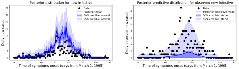
Figure 1: Analysis of real Ebola data with our method. Posterior smoothing distributions for the number of new infectives per day and posterior predictive distributions for the associated observations, i.e., subject to under-reporting. Control measures were introduced on day 70.

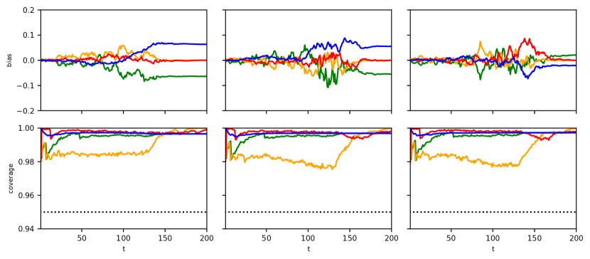
Figure 2: Empirical bias and empirical coverage of nominal $95\%$-credible intervals from $2\times 10^{4}$ simulations over $200$ time steps of the Ebola model. Columns from left to right: $n=5\times 10^{2},5\times 10^{4},5\times 10^{6}$. Top row: bias, bottom row: coverage. Red, yellow, blue, green correspond to $x_{t}^{(i)}$, $i=1,2,3,4$, i.e. susceptible, exposed, infective, recovered.

5.2 Accuracy: filtering bias and credible interval coverage

The purpose of this subsection is to study the accuracy of the approximate filtering distributions obtained from algorithm 2 when applied to the Ebola model described in subsection 5.1. The ground truth parameter values $(\beta,\lambda,\rho,\gamma)$ in the synthetic data experiment were taken together with $q_{t}^{(2,3)}=291/316$, $q_{t}^{(3,4)}=236/316$. We considered three population sizes $n=5\times 10^{2},5\times 10^{4},5\times 10^{6}$, and in each case the initial distribution was $\bm{\pi}_{0}=[1-1/n,1/n,0,0]^{\mathrm{T}}$. For each value of $n$, we simulated $2\times 10^{4}$ data sets from the model, each over $200$ time steps.

To assess accuracy we considered bias and credible-interval coverage. For the former we calculated the empirical bias associated with the mean vector of the approximation to $p(\mathbf{x}_{t}|\mathbf{Y}_{1:t})$ obtained from algorithm 2 as an estimator of $\mathbf{x}_{t}$. For the latter we calculated the empirical coverage of the nominal $95\%$-credible interval for the marginal over each $x_{t}^{(i)}$, $i=1,2,3,4$. For the true (i.e. approximation-free) filtering distributions, asymptotically in the number of simulated data sets the bias would be zero and the coverage would be $95\%$.

Figure 2 shows that for all three values of $n$, the bias at every time step and for every compartment is less than $0.1$ in magnitude. This shows the approximation is very accurate: the true values of $x_{t}^{(i)}$, $i=1,2,3,4$ are always integers, and a bias less than $0.5$ in magnitude means that, on average, if the estimated number of individuals is rounded to the nearest integer, the true number of individuals is recovered. The credible interval coverage reported in figure 2 shows that the approximate filtering distributions tend to over-represent uncertainty: the empirical coverage at all time steps for all compartments of the nominal $95\%$ interval is is between $97\%$ and $100\%$. The bias and coverage appear robust to population size.

Figure 3: Results for the COVID-19 model using our methods. Red line is date at which travel restrictions were introduced. Top: estimated reproduction number. Middle row: estimated daily new confirmed cases in Wuhan (left) and internationally (right), both with in-sample data by date of symptom onset. Bottom row, left: estimated new symptomatic but possibly unconfirmed cases (left axis) and out-of-sample new confirmed cases data (right axis); right: estimated confirmed international cases by date of confirmation, and out-of-sample data.

5.3 Estimating the time-varying reproduction number of COVID-19 in Wuhan, China

A compartmental model for estimating the time-varying reproduction number of COVID-19 in Wuhan, China, has recently been published in Kucharski et al. (2020). The model has 15 compartments: susceptibles in Wuhan become exposed and either stay in Wuhan or depart internationally, then in either case pass through further stages being exposed, infective, symptomatic and confirmed. The transmission rate is modelled as time-varying $(\beta_{t})_{t\geq 0}$, a-priori by a geometric random walk, and $\beta_{t}$ is considered proportional to the reproductive number $R_{t}$. Kucharski et al. (2020) proposed a Sequential Monte Carlo (SMC) algorithm to estimate $(R_{t})_{t\geq 0}$ which weights samples of $(\beta_{t})_{t\geq 0}$ by the likelihood of the associated ODE solution under a Poisson observation model. Our methods can be used to replace their ODE model with a discrete-time stochastic version of the compartmental model, and with their Poisson model replaced our binomial observation model from section 3.3. Our version of the SMC algorithm weights samples of $(\beta_{t})_{t\geq 0}$ by their approximate marginal likelihoods, computed using our multinomial filtering techniques. We jointly analyzed two of three data sets from Kucharski et al. (2020): daily counts of new infectives by date of symptom onset in Wuhan, and internationally exported from Wuhan.

Figure 3 shows our results in the format of Kucharski et al. (2020). Compared to results obtained using their ODE model (see supplementary material), our estimates of $R_{t}$ are generally lower, and closer $1$ for the period after travel restrictions are introduced; and our credible intervals for the in-sample plots are generally wider, reflecting the stochastic nature of our compartmental model. In the bottom two plots our posteriors are mostly concentrated on lower values than those from the method of Kucharski et al. (2020).

Acknowledgements

Nick Whiteley was supported by a Turing Fellowship from the Alan Turing Institute, GW4 and Jean Golding Institute seed-corn funding and thanks Lawrence Murray for discussions about epidemic models. Lorenzo Rimella was supported the Alan Turing Institute PhD Enrichment Scheme.

Appendix A Reader’s guide to the appendices

Appendix B discusses some of the shortcomings of deterministic compartmental models, expanding on the discussion in section 2.1. Appendix C contains proofs of lemmas 1 and 2, plus corresponding results and proofs for the observation model from section 3.3, and derivation of smoothing algorithms. Appendix D provides additional details and numerical results for the Ebola example in section 5.1. Additional details and numerical results for the COVID-19 example in section 5.3 are given in appendix E.

Appendix B Stochastic vs. deterministic SEIR models

Perhaps the most widely applied formulation of a compartmental model is as a system of ordinary differential equations.

SEIR example.

For a population of size $n$, the SEIR ODE model is:

$$\frac{\mathrm{d}S}{\mathrm{d}t}=-\frac{\beta SI}{n},\qquad\frac{\mathrm{d}E}{\mathrm{d}t}=\frac{\beta SI}{n}-\rho E,\qquad\frac{\mathrm{d}I}{\mathrm{d}t}=\rho E-\gamma I,\qquad\frac{\mathrm{d}R}{\mathrm{d}t}=\gamma I,$$ (18)

initialized with nonnegative integers in each of the compartments $(S_{0},E_{0},I_{0},R_{0})$ such that $S_{0}+E_{0}+I_{0}+R_{0}=n$.

The most obvious drawback of ODE models is that, once model parameters and the initial population are fixed, any discrepancy between observed data and the solution of the ODE has to be explained as observation error, which is a serious restriction from a modelling point of view. In practice one can try to estimate unknown parameters and/or the initial condition by numerically minimizing this discrepancy, e.g. under squared error loss. Standard errors for parameter estimates can be derived using asymptotic theory for nonlinear least squares, but calculation of them in practice involves numerical differentiation of the ODE solution flow w.r.t. parameters [Chowell et al., 2004]. When a probabilistic observation model is specified, Bayesian approaches allow for uncertainty quantification over parameters via posterior distributions, but evaluating the likelihood function for model parameters still involves numerical solution of the ODE.

Figure 4 shows simulation output for the proportion of infective individuals in the discrete-time SEIR model with $n=10^{2},10^{3},10^{5},10^{7}$ and initial conditions $(S_{0},E_{0},I_{0},R_{0})=(n-1,1,0,0)$, with $\beta=0.8$, $\rho=1/9$ and $\gamma=0.2$. It is evident that the sample paths become smoother as $n$ grows, but there is still substantial variability across sample paths even with $n=10^{7}$. This can be explained by the fact that since $(E_{0},I_{0})=(1,0)$ independently of $n$, the numbers of exposed and infective individuals in the first few time periods of the epidemic are typically very small, despite the fact that the overall population size may be large, and the statistical variability associated with these small numbers has a lasting effect on the overall timing of the outbreak.

To explain how this relates to ODE limits, for $n\geq 1$ and initial proportions of the population $(s_{0},e_{0},i_{0},r_{0})$, i.e., $s_{0}+e_{0}+i_{0}+r_{0}=1$, let us write $\mathcal{D}_{n}(s_{0},e_{0},i_{0},r_{0})$ for the collection of ODEs in (18) together with the initial condition $(ns_{0},ne_{0},ni_{0},nr_{0})$. It can be checked by substitution that $t\mapsto(S_{t},E_{t},I_{t},R_{t})$ is a solution of $\mathcal{D}_{1}(s_{0},e_{0},i_{0},r_{0})$ if and only if $t\mapsto(nS_{t},nE_{t},nI_{t},nR_{t})$ is a solution of $\mathcal{D}_{n}(s_{0},e_{0},i_{0},r_{0})$. Thus we see that $n$ plays a trivial role in the ODE model: it is just a scaling factor for the solution.

The limit theorems of Kurtz [1970, 1971] applied in this situation pertain to the probabilistic convergence on a finite time-window as $n\to\infty$ of the path of the continuous-time SEIR Markov process with initial condition $(S_{0},E_{0},I_{0},R_{0})=(n-1,1,0,0)$ and compartment counts normalized by $n$, to the solution of $\mathcal{D}_{1}(s_{0},e_{0},i_{0},r_{0})$, where $(s_{0},e_{0},i_{0},r_{0})=\lim_{n\to\infty}(n-1,1,0,0)/n=(1,0,0,0)$. However in the solution of $\mathcal{D}_{1}(1,0,0,0)$, the exposed and infective compartments are always empty, i.e. an epidemic never occurs. This can be reconciled with figure 4 by observing that there the peak in the number of infectives typically occurs later as $n$ grows: the limiting $n\to\infty$ case is that in which a peak never occurs.

This illustrates that sequences of well-behaved stochastic models can have ODE limits which are unrealistic to the point of being pathological, and therefore these limits are not always a sensible justification for using ODE models.

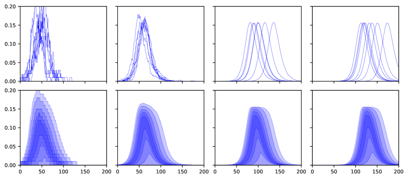
Figure 4: Proportion of infective individuals against time in simulations from the discrete-time stochastic SEIR model with $\beta=0.8$, $\rho=1/5$, $\gamma=1/9$ and $h=1$ over $200$ time steps. Columns left to right: $n=10^{2},10^{3},10^{5},10^{7}$ and initial conditions $(S_{0},E_{0},I_{0},R_{0})=(n-1,1,0,0)$. Top row: 10 realizations from the model. Bottom row: at each time step shaded regions indicate percentile intervals of the form $[\alpha,1-\alpha]\times 100\%$, for $\alpha=0.05,0.1,0.2,0.3,0.4$ estimated from $10^{4}$ realizations from the model.

Appendix C Supplementary information about multinomial filtering and smoothing

C.1 Proofs of Lemmas 1 and 2

Proof of Lemma 1.

Since $\mu$ is the probability mass function associated with $\mathrm{Mult}(n,\bm{\pi})$, $\mathbb{E}_{\mu}[\bm{\eta}(\mathbf{x})]=\bm{\pi}$, so we need to prove that $\sum_{\mathbf{x}\in\mathcal{S}_{m,n}}\mu(\mathbf{x})M_{t}(\mathbf{x},\bm{\pi},\cdot)$ is the probability mass function associated with $\mathrm{Mult}(n,\bm{\pi}^{\mathrm{T}}\mathbf{K}_{t,\bm{\pi}})$. We shall achieve this using the unique characterization of the probability mass function by its moment generating function.

With $\mathbf{x}\sim\mu$, let $\widetilde{\mathbf{x}}\sim M_{t}(\mathbf{x},\bm{\pi},\cdot)$, so by construction $\sum_{\mathbf{x}\in\mathcal{S}_{m,n}}\mu(\mathbf{x})M_{t}(\mathbf{x},\bm{\pi},\cdot)$ is the marginal probability mass function of $\widetilde{\mathbf{x}}$. Therefore by the definition of $M_{t}$ in section 4.1, $\widetilde{\mathbf{x}}=(\mathbf{1}_{m}^{\mathrm{T}}\mathbf{Z})^{\mathrm{T}}$, where the rows of $\mathbf{Z}$ are conditionally independent given $\mathbf{x}$, and the conditional distribution of the $i$th row of $\mathbf{Z}$ given $\mathbf{x}$ is $\mathrm{Mult}(x^{(i)},\mathbf{K}_{t,\bm{\pi}}^{(i,\cdot)})$. Using these facts, the moment generating function of $\widetilde{\mathbf{x}}$ can be written:

$$\mathbb{E}\left[\exp(\widetilde{\mathbf{x}}^{\mathrm{T}}\mathbf{b})\right] =\mathbb{E}\left[\exp(\mathbf{1}_{m}^{\mathrm{T}}\mathbf{Z}\mathbf{b})\right]$$

$$=\mathbb{E}\left[\exp\left(\sum_{i,j=1}^{m}Z^{(i,j)}b^{(j)}\right)\right]$$

$$=\mathbb{E}\left[\mathbb{E}\left[\left.\exp\left(\sum_{i,j=1}^{m}Z^{(i,j)}b^{(j)}\right)\right|\mathbf{x}\right]\right]$$

$$=\mathbb{E}\left[\prod_{i=1}^{m}\mathbb{E}\left[\left.\exp\left(\sum_{j=1}^{m}Z^{(i,j)}b^{(j)}\right)\right|x^{(i)}\right]\right].$$ (19)

Now we use the fact that, again by definition of $M_{t}$, $\mathbb{E}\left[\left.\exp\left(\sum_{j=1}^{m}Z^{(i,j)}b^{(j)}\right)\right|x^{(i)}\right]$ is the m.g.f. of $\text{Mult}(x^{(i)},\mathbf{K}_{t,\bm{\pi}}^{(i,\cdot)})$, where $\mathbf{K}_{t,\bm{\pi}}$ has elements $k_{t,\bm{\pi}}^{(i,j)}$, i.e. :

$$\mathbb{E}\left[\left.\exp\left(\sum_{j=1}^{m}Z^{(i,j)}b^{(j)}\right)\right|x^{(i)}\right]=\left(\sum_{j=1}^{m}k_{t,\bm{\pi}}^{(i,j)}e^{b^{(j)}}\right)^{x^{(i)}}.$$

Substituting this into (19) and then using $\mathbf{x}\sim\mu=\text{Mult}(n,\bm{\mathbf{\pi}})$,

$$\mathbb{E}\left[\exp(\widetilde{\mathbf{x}}^{\mathrm{T}}\mathbf{b})\right] =\mathbb{E}\left[\prod_{i=1}^{m}\mathbb{E}\left[\left.\exp\left(\sum_{j=1}^{m}Z^{(i,j)}b^{(j)}\right)\right|x^{(i)}\right]\right]=\mathbb{E}\left[\prod_{i=1}^{m}\left(\sum_{j=1}^{m}k_{t,\bm{\pi}}^{(i,j)}e^{b^{(j)}}\right)^{x^{(i)}}\right]$$

$$=\sum_{(x^{(1)},\ldots,x^{(m)})\in\mathcal{S}_{m,n}}n!\prod_{i=1}^{m}\frac{(\pi^{(i)})^{x^{(i)}}}{x^{(i)}!}\left(\sum_{j=1}^{m}k_{t,\bm{\pi}}^{(i,j)}e^{b^{(j)}}\right)^{x^{(i)}}$$

$$=\sum_{(x^{(1)},\ldots,x^{(m)})\in\mathcal{S}_{m,n}}n!\prod_{i=1}^{m}\frac{1}{x^{(i)}!}\left(\sum_{j=1}^{m}\pi^{(i)}k_{t,\bm{\pi}}^{(i,j)}e^{b^{(j)}}\right)^{x^{(i)}}$$

$$=\left(\sum_{i=1}^{m}\sum_{j=1}^{m}\pi^{(i)}k_{t,\bm{\pi}}^{(i,j)}e^{b^{(j)}}\right)^{n}=\left(\sum_{j=1}^{m}(\bm{\pi}^{\mathrm{T}}\mathbf{K}_{t,\bm{\pi}})^{(j)}e^{b^{(j)}}\right)^{n},$$

where the penultimate equality holds by the multinomial theorem. The proof is completed by noticing that $\left(\sum_{j=1}^{m}(\bm{\pi}^{\mathrm{T}}\mathbf{K}_{t,\bm{\pi}})^{(j)}e^{b^{(j)}}\right)^{n}$ is the moment generating function of $\text{Mult}(n,\bm{\pi}^{\mathrm{T}}\mathbf{K}_{t,\bm{\pi}})$. ∎

Proof of Lemma 2.

Under the distributional assumptions in the statement of the lemma, for $\mathbf{x}\in\mathcal{S}_{m,n}$,

$$p(\mathbf{x})=\frac{n!}{\prod_{j=1}^{m}x^{(j)}!}\prod_{j=1}^{m}(\pi^{(j)})^{x^{(j)}},$$

and for $0\leq y^{(j)}\leq x^{(j)},\,j=1,\ldots,m$,

$$p(\mathbf{y}|\mathbf{x})=\prod_{j=1}^{m}\frac{x^{(j)}!}{y^{(j)}!(x^{(j)}-y^{(j)})!}(q^{(j)})^{y^{(j)}}(1-q^{(j)})^{x^{(j)}-y^{(j)}}.$$

Therefore

$$p(\mathbf{x},\mathbf{y})=n!\prod_{j=1}^{m}\frac{(\pi^{(j)})^{x^{(j)}}(q^{(j)})^{y^{(j)}}(1-q^{(j)})^{x^{(j)}-y^{(j)}}}{y^{(j)}!(x^{(j)}-y^{(j)})!},$$ (20)

and

$$p(\mathbf{y}) =\sum_{\{x^{(j)}:x^{(j)}\geq y^{(j)},\sum_{j}x^{(j)}=n\}}n!\prod_{j=1}^{m}\frac{(\pi^{(j)})^{x^{(j)}}(q^{(j)})^{y^{(j)}}(1-q^{(j)})^{x^{(j)}-y^{(j)}}}{y^{(j)}!(x^{(j)}-y^{(j)})!}$$

$$=n!\left(\prod_{j=1}^{m}\frac{(q^{(j)})^{y^{(j)}}(\pi^{(j)})^{y^{(j)}}}{y^{(j)}!}\right)$$

$$\qquad\times\sum_{\{x^{(j)}:x^{(j)}\geq y^{(j)},\sum_{j}x^{(j)}=n\}}\left(\prod_{j=1}^{m}\frac{(\pi^{(j)})^{x^{(j)}-y^{(j)}}(1-q^{(j)})^{x^{(j)}-y^{(j)}}}{(x^{(j)}-y^{(j)})!}\right)$$

$$=n!\left(\prod_{j=1}^{m}\frac{(q^{(j)})^{y^{(j)}}(\pi^{(j)})^{y^{(j)}}}{y^{(j)}!}\right)\frac{\left(\sum_{j=1}^{m}\pi^{(j)}(1-q^{(j)})\right)^{n-\sum_{j=1}^{m}y^{(j)}}}{(n-\sum_{j=1}^{m}y^{(j)})!},$$ (21)

where the final equality holds by the multinomial theorem. Dividing (20) by (21) gives

$$p(\mathbf{x}|\mathbf{y}) =\left(n-\sum_{j=1}^{m}y^{(j)}\right)!\prod_{j=1}^{m}\frac{1}{(x^{(j)}-y^{(j)})!}\left(\frac{\pi^{(j)}(1-q^{(j)})}{\sum_{i=1}^{m}\pi^{(i)}(1-q^{(i)})}\right)^{x^{(j)}-y^{(j)}},$$

which is the probability mass function of $\mathbf{y}+\mathbf{x}^{\star}$ given in the statement of the lemma. ∎

Remark 1.

The probability mass function in (21) has the interpretation of being a multinomial distribution over $n+1$ compartments, where the count variable associated with the $(m+1)$th compartment is $n-\sum_{j=1}^{m}y^{(j)}$.

C.2 Approximating the prediction and update operations for $(\mathbf{Z}_{t},\mathbf{Y}_{t})_{t\geq 1}$

Algorithm 2 is derived from lemma 3 and 4. Given $\mathbf{Z}$ and $\bm{\eta}$, let $\overline{M}_{t}(\mathbf{Z},\bm{\eta},\cdot)$ be the probability mass function of a random $m\times m$ matrix, say $\widetilde{\mathbf{Z}}$, such that $\mathbf{1}_{m}^{\mathrm{T}}\mathbf{Z}=(\widetilde{\mathbf{Z}}\mathbf{1}_{m})^{\mathrm{T}}$ with probability $1$, and such that given the row-sums $\widetilde{\mathbf{Z}}\mathbf{1}_{m}$, rows of $\widetilde{\mathbf{Z}}$ are independent and the conditional distribution of the $i$th row is $\mathrm{Mult}(x^{(i)},\mathbf{K}_{t,\bm{\eta}}^{(i,\cdot)})$ where $\mathbf{x}^{\mathrm{T}}=\mathbf{1}_{m}^{\mathrm{T}}\mathbf{Z}$. So by construction $\overline{M}_{t}(\mathbf{Z}_{t-1},\bm{\eta}(\mathbf{1}_{m}^{\mathrm{T}}\mathbf{Z}_{t-1}),\mathbf{Z}_{t})$ gives the transition probabilities of the Markov chain $(\mathbf{Z}_{t})_{t\geq 1}$ defined in section 3.1.

Lemma 3.

If for a given $m\times m$ matrix $\mathbf{P}$, $\overline{\mu}$ is the probability mass function associated with $\mathrm{Mult}(n,\mathbf{P})$ and $\mathbb{E}_{\overline{\mu}}[\bm{\eta}(\mathbf{1}_{m}^{\mathrm{T}}\mathbf{Z})]$ is the expected value of $\mathbf{1}_{m}^{\mathrm{T}}\mathbf{Z}$ when $\mathbf{Z}\sim\mathrm{Mult}(n,\mathbf{P})$, then $\sum_{\mathbf{Z}}\overline{\mu}(\mathbf{Z})\overline{M}_{t}(\mathbf{Z},\mathbb{E}_{\overline{\mu}}[\bm{\eta}(\mathbf{1}_{m}^{\mathrm{T}}\mathbf{Z})],\cdot)$ is the probability mass function associated with $\mathrm{Mult}(n,(\bm{\pi}\otimes\mathbf{1}_{m})\circ\mathbf{K}_{t,\bm{\pi}})$ where $\bm{\pi}^{\mathrm{T}}=\mathbf{1}_{m}^{\mathrm{T}}\mathbf{P}$.

Proof.

The proof is similar to the proof of Lemma 1, so some steps and commentary are omitted. Note $\mathbb{E}_{\overline{\mu}}[\bm{\eta}((\mathbf{1}_{m}^{\mathrm{T}}\mathbf{Z})^{\mathrm{T}})]=(\mathbf{1}_{m}^{\mathrm{T}}\mathbf{P})^{\mathrm{T}}=\bm{\pi}$, and let $\widetilde{\mathbf{Z}}\sim\overline{M}(\mathbf{Z},\bm{\pi},\cdot)$. The moment generating function of $\mathbf{\widetilde{Z}}$ is:

$$\mathbb{E}[\exp(\mathbf{1}_{m}^{\mathrm{T}}(\mathbf{\widetilde{Z}}\circ\mathbf{B})\mathbf{1}_{m})] =\mathbb{E}\left[\prod_{i=1}^{m}\exp\left(\sum_{j=1}^{m}\widetilde{z}^{(i,j)}b^{(i,j)}\right)\right]$$

$$=\mathbb{E}\left[\mathbb{E}\left[\left.\prod_{i=1}^{m}\exp\left(\sum_{j=1}^{m}\widetilde{z}^{(i,j)}b^{(i,j)}\right)\right|\mathbf{Z}\right]\right]$$

$$=\mathbb{E}\left[\prod_{i=1}^{m}\mathbb{E}\left[\left.\exp\left(\sum_{j=1}^{m}\widetilde{z}^{(i,j)}b^{(i,j)}\right)\right|(\mathbf{1}_{m}^{\mathrm{T}}\mathbf{Z})^{(i)}\right]\right]$$

$$=\mathbb{E}\left[\prod_{i=1}^{m}\left(\sum_{j=1}^{m}k_{t,\bm{\pi}}^{(i,j)}b^{(i,j)}\right)^{(\mathbf{1}_{m}^{\mathrm{T}}\mathbf{Z})^{(i)}}\right]$$

$$=n!\sum_{(x^{(1)},\ldots,x^{(m)})\in\mathcal{S}_{m,n}}\prod_{i=1}^{m}\frac{(\pi^{(i)})^{x^{(i)}}}{x^{(i)}!}\left(\sum_{j=1}^{m}k_{t,\bm{\pi}}^{(i,j)}e^{b^{(i,j)}}\right)^{x^{(i)}}$$

$$=\left(\sum_{i=1}^{m}\sum_{j=1}^{m}\pi^{(i)}k_{t,\bm{\pi}}^{(i,j)}e^{b^{(i,j)}}\right)^{n}.$$

∎

Lemma 4.

Suppose that $\mathbf{Z}\sim\mathrm{Mult}(n,\mathbf{P})$ for a given $m\times m$ matrix $\mathbf{P}$, and given $\mathbf{Z}$, $\mathbf{Y}$ is a matrix with conditionally independent entries distributed: $y^{(i,j)}\sim\mathrm{Bin}(z^{(i,j)},q^{(i,j)})$. Then the conditional distribution of $\mathbf{Z}$ given $\mathbf{Y}$ is equal to that of $\mathbf{Y}+\mathbf{Z}^{\star}$ where

$$\mathbf{Z}^{\star}\sim\mathrm{Mult}\left(n-\mathbf{1}_{m}^{\mathrm{T}}\mathbf{Y}\mathbf{1}_{m},\frac{\mathbf{P}\circ(\mathbf{1}_{m}\otimes\mathbf{1}_{m}-\mathbf{Q})}{1-\mathbf{1}_{m}^{\mathrm{T}}(\mathbf{P}\circ\mathbf{Q})\mathbf{1}_{m}}\right)$$

and

$$\mathbb{E}\left[\mathbf{Z}|\mathbf{Y}\right]=\mathbf{Y}+(n-\mathbf{1}_{m}^{\mathrm{T}}\mathbf{Y}\mathbf{1}_{m})\frac{\mathbf{P}\circ(\mathbf{1}_{m}\otimes\mathbf{1}_{m}-\mathbf{Q})}{1-\mathbf{1}_{m}^{\mathrm{T}}(\mathbf{P}\circ\mathbf{Q})\mathbf{1}_{m}}.$$

Moreover

$$\log p(\mathbf{Y})=\log(n!)+\mathbf{1}_{m}^{\mathrm{T}}(\mathbf{Y}\circ\log\mathbf{P})\mathbf{1}_{m}+\mathbf{1}_{m}^{\mathrm{T}}(\mathbf{Y}\circ\log\mathbf{Q})\mathbf{1}_{m}-\mathbf{1}_{m}^{\mathrm{T}}\log(\mathbf{Y}!)\mathbf{1}_{m}$$

$$\qquad+(n-\mathbf{1}_{m}^{\mathrm{T}}\mathbf{Y}\mathbf{1}_{m})\log(1-\mathbf{1}_{m}^{\mathrm{T}}(\mathbf{P}\circ\mathbf{Q})\mathbf{1}_{m})-\log((n-\mathbf{1}_{m}^{\mathrm{T}}\mathbf{Y}\mathbf{1}_{m})!).$$

The proof is very similar to the proof of Lemma 2 so is omitted.

C.3 Smoothing with the observation model from section 3.2

Assuming that algorithm 1 has already been run up to a given time $t$, our objective in this section is to derive algorithm 3, from which we take the approximations:

$$p(\mathbf{x}_{s}|\mathbf{y}_{1:t})\approx\mathrm{Mult}(n,\bm{\pi}_{s|t}),\qquad p(\mathbf{Z}_{s}|\mathbf{y}_{1:t})\approx\mathrm{Mult}(n,(\mathbf{1}_{m}\otimes\bm{\pi}_{s|t})\circ\mathbf{L}_{s-1}^{\mathrm{T}}).$$

Algorithm 3 Multinomial smoothing with observations derived from $(\mathbf{x}_{t})_{t\geq 1}$

1:for $s=t-1,\ldots,0$ do

2:     let $\mathbf{L}_{s}$ be the matrix with elements $l_{s}^{(i,j)}\leftarrow\pi_{s|s}^{(j)}\,k_{s+1,\bm{\pi}_{s|s}}^{(j,i)}/(\bm{\pi}_{s|s}^{\mathrm{T}}\mathbf{K}_{s+1,\bm{\pi}_{s|s}})^{(i)}$

3:     $\bm{\pi}_{s|t}\leftarrow(\bm{\pi}_{s+1|t}^{\mathrm{T}}\mathbf{L}_{s})^{\mathrm{T}}$

4:end for

We start by considering the identities:

$$p(\mathbf{x}_{0:t}|\mathbf{y}_{1:t})=p(\mathbf{x}_{t}|\mathbf{y}_{1:t})\prod_{s=0}^{t-1}p(\mathbf{x}_{s}|\mathbf{x}_{s+1},\mathbf{y}_{1:s})$$

$$p(\mathbf{x}_{s}|\mathbf{x}_{s+1},\mathbf{y}_{1:s})=\frac{p(\mathbf{x}_{s}|\mathbf{y}_{1:s})p(\mathbf{x}_{s+1}|\mathbf{x}_{s})}{p(\mathbf{x}_{s+1}|\mathbf{y}_{1:s})}$$ (22)

$$p(\mathbf{x}_{s+1}|\mathbf{y}_{1:s})=\sum_{\mathbf{x}_{s}\in\mathcal{S}_{m,n}}p(\mathbf{x}_{s}|\mathbf{y}_{1:s})p(\mathbf{x}_{s+1}|\mathbf{x}_{s}),$$

with the conventions $p(\mathbf{x}_{0}|\mathbf{x}_{1},\mathbf{y}_{1:0})\equiv p(\mathbf{x}_{0}|\mathbf{x}_{1})$, $p(\mathbf{x}_{0}|\mathbf{y}_{1:0})\equiv p(\mathbf{x}_{0})$. The smoothing distributions $p(\mathbf{x}_{s}|\mathbf{y}_{1:t})$, $s=0,\ldots,t$, satisfy the ‘backward’ recursion.

$$\sum_{\mathbf{x}_{s+1}\in\mathcal{S}_{m,n}}p(\mathbf{x}_{s+1}|\mathbf{y}_{1:t})p(\mathbf{x}_{s}|\mathbf{x}_{s+1},\mathbf{y}_{1:s})=p(\mathbf{x}_{s}|\mathbf{y}_{1:t}).$$ (23)

All these formulae are standard identities for hidden Markov models [Briers et al., 2010].

In order to approximate (23) we approximate each of the terms $p(\mathbf{x}_{s}|\mathbf{x}_{s+1},\mathbf{y}_{1:s})$. Consider first the numerator in (22). Recall from section 4.1 that the transition probabilities of the $(\mathbf{x}_{s})_{s\geq 0}$ process can be written in terms of $(M_{s})_{s\geq 1}$, so:

$$p(\mathbf{x}_{s}|\mathbf{y}_{1:s})p(\mathbf{x}_{s+1}|\mathbf{x}_{s})=p(\mathbf{x}_{s}|\mathbf{y}_{1:s})M_{s+1}(\mathbf{x}_{s},\bm{\eta}(\mathbf{x}_{s}),\mathbf{x}_{s+1}).$$ (24)

We replace $p(\mathbf{x}_{s}|\mathbf{y}_{1:s})$ in (24) by its multinomial approximation $\mathrm{Mult}(n,\bm{\pi}_{s|s})$ obtained using algorithm 1, and replace $\bm{\eta}(\mathbf{x}_{s})$ in (24) by its expected value under this multinomial distribution, i.e. $\bm{\pi}_{s|s}$, to give

$$p(\mathbf{x}_{s}|\mathbf{x}_{s+1},\mathbf{y}_{1:s})\approx\frac{\mu_{s|s}(\mathbf{x}_{s})M_{s+1}(\mathbf{x}_{s},\bm{\pi}_{s|s},\mathbf{x}_{s+1})}{\sum_{\mathbf{z}\in\mathcal{S}_{m,n}}\mu_{s|s}(\mathbf{z})M_{s+1}(\mathbf{z},\bm{\pi}_{s|s},\mathbf{x}_{s+1})},$$ (25)

where $\mu_{s|s}(\cdot)$ is the probability mass function associated with $\mathrm{Mult}(n,\bm{\pi}_{s|s})$.

Lemma 5.

With $\mathbf{x}_{s+1}$ considered fixed, the function which maps $\mathbf{x}_{s}$ to the right hand side of (25) is the probability mass function associated with $\mathbf{1}_{m}^{\mathrm{T}}\widetilde{\mathbf{Z}}$, where $\widetilde{\mathbf{Z}}$ is an $m\times m$ random matrix whose $i$th row has distribution $\mathrm{Mult}(x_{s+1}^{(i)},\mathbf{L}_{s}^{(i,\cdot)})$ and $\mathbf{L}_{s}$ is the row-stochastic matrix with entries

$$l_{s}^{(i,j)}=\frac{\pi_{s|s}^{(j)}\,k_{s+1,\bm{\pi}_{s|s}}^{(j,i)}}{(\bm{\pi}_{s|s}^{\mathrm{T}}\mathbf{K}_{s+1,\bm{\pi}_{s|s}})^{(i)}},$$

where $k_{s+1,\bm{\pi}_{s|s}}^{(i,j)}$ are the elements of $\mathbf{K}_{s+1,\bm{\pi}_{s|s}}$.

Proof.

Recalling the definition of $M_{s+1}$ from section 4.1, the numerator in (25) is:

$$\mu_{s|s}(\mathbf{x}_{s})M_{s+1}(\mathbf{x}_{s},\bm{\pi}_{s|s},\mathbf{x}_{s+1})$$

$$=\left(n!\prod_{i=1}^{m}\frac{(\pi_{s|s}^{(i)})^{x_{s}^{(i)}}}{x_{s}^{(i)}!}\right)\left(\sum_{\mathbf{Z}\in\mathcal{T}_{m,n}(\mathbf{x}_{s},\mathbf{x}_{s+1})}\prod_{i=1}^{m}x_{s}^{(i)}!\prod_{j=1}^{m}\frac{(k_{s+1,\bm{\pi}_{s|s}}^{(i,j)})^{z^{(i,j)}}}{z^{(i,j)}!}\right)$$

$$=n!\left(\prod_{i=1}^{m}(\pi_{s|s}^{(i)})^{x_{s}^{(i)}}\right)\sum_{\mathbf{Z}\in\mathcal{T}_{m,n}(\mathbf{x}_{s},\mathbf{x}_{s+1})}\prod_{i,j=1}^{m}\frac{(k_{s+1,\bm{\pi}_{s|s}}^{(i,j)})^{z^{(i,j)}}}{z^{(i,j)}!}$$

$$=n!\sum_{\mathbf{Z}\in\mathcal{T}_{m,n}(\mathbf{x}_{s},\mathbf{x}_{s+1})}\prod_{i,j=1}^{m}\frac{(\pi_{s|s}^{(i)})^{z^{(i,j)}}(k_{s+1,\bm{\pi}_{s|s}}^{(i,j)})^{z^{(i,j)}}}{z^{(i,j)}!},$$ (26)

where $\mathcal{T}_{m,n}(\mathbf{x}_{s},\mathbf{x}_{s+1})$ is the set of $m\times m$ matrices, say $\mathbf{Z}$, with nonnegative entries such that $\mathbf{Z}\mathbf{1}_{m}=\mathbf{x}_{s}$, $(\mathbf{1}_{m}^{\mathrm{T}}\mathbf{Z})=\mathbf{x}_{s+1}^{\mathrm{T}}$, and $\mathbf{1}_{m}^{\mathrm{T}}\mathbf{Z}\mathbf{1}_{m}=n$.

Now in order to derive an expression for the the denominator in (25), observe that (26) can be disintegrated to give:

$$n!\prod_{i,j=1}^{m}\frac{(\pi_{s|s}^{(i)})^{z^{(i,j)}}(k_{s+1,\bm{\pi}_{s|s}}^{(i,j)})^{z^{(i,j)}}}{z^{(i,j)}!},$$

which is the probability mass function of $\mathbf{Z}\sim\mathrm{Mult}(n,(\bm{\pi}_{s|s}\otimes\mathbf{1}_{m})\circ\mathbf{K}_{s+1,\bm{\pi}_{s|s}})$. Therefore using the fact the marginal of this multinomial distribution over $\mathbf{1}_{m}^{\mathrm{T}}\mathbf{Z}$ is $\mathrm{Mult}(n,\bm{\pi}_{s|s}^{\mathrm{T}}\mathbf{K}_{s+1,\bm{\pi}_{s|s}})$, the denominator in (25) is

$$\sum_{\mathbf{x}_{s}\in\mathcal{S}_{m,n}}\mu_{s|s}(\mathbf{x}_{s})M_{s+1}(\mathbf{x}_{s},\bm{\pi}_{s|s},\mathbf{x}_{s+1})=n!\prod_{j=1}^{m}\frac{((\bm{\pi}_{s|s}^{\mathrm{T}}\mathbf{K}_{s+1,\bm{\pi}_{s|s}})^{(j)})^{x_{s+1}^{(j)}}}{x_{s+1}^{(j)}!}.$$ (27)

Dividing (26) by (27) gives:

$$\sum_{\mathbf{Z}\in\mathcal{T}_{m,n}(\mathbf{x}_{s},\mathbf{x}_{s+1})}\prod_{i=1}^{m}x_{s+1}^{(j)}!\prod_{j=1}^{m}\left(\frac{\pi_{s|s}^{(i)}\,k_{s+1,\bm{\pi}_{s|s}}^{(i,j)}}{(\bm{\pi}_{s|s}^{\mathrm{T}}\mathbf{K}_{s+1,\bm{\pi}_{s|s}})^{(j)}}\right)^{z^{(i,j)}}\frac{1}{z^{(i,j)}!}.$$

Re-writing this sum with the change of variable $\widetilde{\mathbf{Z}}\coloneqq\mathbf{Z}^{\mathrm{T}}$ and interchanging $i$ and $j$ yields the result.

∎

Now considering (23) and the approximation (25), define the probability mass functions:

$$\mu_{s|t}(\mathbf{x}_{s})\coloneqq\sum_{\mathbf{x}_{s+1}\in\mathcal{S}_{m,n}}\mu_{s+1|t}(\mathbf{x}_{s+1})\frac{\mu_{s|s}(\mathbf{x}_{s})M_{s+1}(\mathbf{x}_{s},\bm{\pi}_{s|s},\mathbf{x}_{s+1})}{\sum_{\mathbf{z}\in\mathcal{S}_{m,n}}\mu_{s|s}(\mathbf{z})M_{s+1}(\mathbf{z},\bm{\pi}_{s|s},\mathbf{x}_{s+1})},\quad s<t,$$

recalling from (25) that $\mu_{t|t}(\cdot)$ is the probability mass function associated with $\mathrm{Mult}(n,\bm{\pi}_{t|t})$.

Lemma 6.

For $0\leq s\leq t$, $\mu_{s|t}(\cdot)$ is the probability mass function associated with $\mathrm{Mult}(n,\bm{\pi}_{s|t})$, where $\bm{\pi}_{s|t}$ is computed as per algorithm 3.

Proof.

The result can be proved by induction. The induction is initialized using the fact that $\mu_{t|t}(\cdot)$ is by definition the probability mass function associated with $\mathrm{Mult}(n,\bm{\pi}_{t|t})$, and then proceeds by combining the result of lemma 5 with moment generating function techniques similar to those used in the proof of lemma 1. The details are omitted to avoid repetition. ∎

C.4 Smoothing with the observation model from section 3.3

Assuming algorithm 2 has already been run up to a given time $t$, our objective in this section is to derive algorithm 4, from which we take the approximation:

$$p(\mathbf{Z}_{s}|\mathbf{y}_{1:t})\approx\mathrm{Mult}(n,\mathbf{P}_{s|t}).$$

Algorithm 4 Multinomial smoothing with observations derived from $(\mathbf{Z}_{t})_{t\geq 1}$

1:for $s=t-1,\ldots,1$ do

2:     $\bm{\pi}_{s|t}\leftarrow\mathbf{P}_{s+1|t}\mathbf{1}_{m}$

3:     let $\overline{\mathbf{L}}_{s}$ be the matrix with elements $\overline{l}_{s}^{(i,j)}\leftarrow p_{s|s}^{(j,i)}/\pi_{s|s}^{(i)}$

4:     $\mathbf{P}_{s|t}\leftarrow(\mathbf{1}_{m}\otimes\bm{\pi}_{s|t})\circ\overline{\mathbf{L}}_{s}^{\mathrm{T}}$

5:end for

In algorithm 4, $p_{s|s}^{(i,j)}$ are the elements of $\mathbf{P}_{s|s}$ and $\pi_{s|s}^{(i)}$ are the elements of $\bm{\pi}_{s|s}\coloneqq(\mathbf{1}_{m}^{\mathrm{T}}\mathbf{P}_{s|s})^{\mathrm{T}}$, with $\mathbf{P}_{s|s}$ computed in algorithm 2.

Similarly to section C.3, to derive our approximations we start from the fact that $(\mathbf{Z}_{t},\mathbf{Y}_{t})_{t\geq 1}$ is a hidden Markov model, and consider the identities:

$$p(\mathbf{Z}_{1:t}|\mathbf{Y}_{1:t})=p(\mathbf{Z}_{t}|\mathbf{Y}_{1:t})\prod_{s=1}^{t-1}p(\mathbf{Z}_{s}|\mathbf{Z}_{s+1},\mathbf{Y}_{1:s})$$

$$p(\mathbf{Z}_{s}|\mathbf{Z}_{s+1},\mathbf{Y}_{1:s})=\frac{p(\mathbf{Z}_{s}|\mathbf{Y}_{1:s})p(\mathbf{Z}_{s+1}|\mathbf{Z}_{s})}{p(\mathbf{Z}_{s+1}|\mathbf{Y}_{1:s})}$$ (28)

$$p(\mathbf{Z}_{s+1}|\mathbf{Y}_{1:s})=\sum_{\mathbf{Z}_{s}}p(\mathbf{Z}_{s}|\mathbf{Y}_{1:s})p(\mathbf{Z}_{s+1}|\mathbf{Z}_{s}).$$

The backward recursion is in this case:

$$\sum_{\mathbf{Z}_{s+1}}p(\mathbf{Z}_{s+1}|\mathbf{Y}_{1:t})p(\mathbf{Z}_{s}|\mathbf{Z}_{s+1},\mathbf{Y}_{1:s})=p(\mathbf{Z}_{s}|\mathbf{Y}_{1:t}).$$ (29)

Writing $\overline{\mu}_{s|s}(\cdot)$ for the probability mass function associated with $\mathrm{Mult}(n,\mathbf{P}_{s|s})$, our approximation to (28) is:

$$p(\mathbf{Z}_{s}|\mathbf{Z}_{s+1},\mathbf{Y}_{1:s})\approx\frac{\overline{\mu}_{s|s}(\mathbf{Z}_{s})\overline{M}_{s+1}(\mathbf{Z}_{s},\bm{\pi}_{s|s},\mathbf{Z}_{s+1})}{\sum_{\widetilde{\mathbf{Z}}}\overline{\mu}_{s|s}(\widetilde{\mathbf{Z}})\overline{M}_{s+1}(\widetilde{\mathbf{Z}},\bm{\pi}_{s|s},\mathbf{Z}_{s+1})}.$$ (30)

where $\overline{M}_{s+1}$ was introduced in section C.2 and in the setting of (30) has the explicit formula:

$$\overline{M}_{s+1}(\mathbf{Z}_{s},\bm{\pi}_{s|s},\mathbf{Z}_{s+1})=\mathbb{I}[\mathbf{1}_{m}^{\mathrm{T}}\mathbf{Z}_{s}=(\mathbf{Z}_{s+1}\mathbf{1}_{m})^{\mathrm{T}}]\left(\prod_{j=1}^{m}(\mathbf{Z}_{s+1}\mathbf{1}_{m})^{(j)}!\prod_{\ell=1}^{m}\frac{\left(k_{s+1,\bm{\pi}_{s|s}}^{(j,\ell)}\right)^{z_{s+1}^{(j,\ell)}}}{z_{s+1}^{(j,\ell)}!}\right).$$

Lemma 7.

With $\mathbf{Z}_{s+1}$ considered fixed, the function which maps $\mathbf{Z}_{s}$ to the right hand side of (30) is the probability mass function such that the columns of $\mathbf{Z}_{s}$ are independent and the distribution of the $i$th column is $\mathrm{Mult}((\mathbf{Z}_{s+1}\mathbf{1}_{m})^{(i)},\overline{\mathbf{L}}_{s}^{(i,\cdot)})$, where $\overline{\mathbf{L}}_{s}$ is the row-stochastic matrix with entries

$$\overline{l}_{s}^{(i,j)}=p_{s|s}^{(j,i)}/\pi_{s|s}^{(i)}$$

where $p_{s|s}^{(i,j)}$ are the elements of $\mathbf{P}_{s|s}$, and $\pi_{s|s}^{(i)}$ are the elements of $\bm{\pi}_{s|s}\coloneqq(\mathbf{1}_{m}^{\mathrm{T}}\mathbf{P}_{s|s})^{\mathrm{T}}$ with $\mathbf{P}_{s|s}$ computed in algorithm 2.

Proof.

For the numerator in (30) is

$$\overline{\mu}_{s|s}(\mathbf{Z}_{s})\overline{M}_{s+1}(\mathbf{Z}_{s},\bm{\pi}_{s|s},\mathbf{Z}_{s+1})$$

$$=\left(n!\prod_{i,j=1}^{m}\frac{(p_{s|s}^{(i,j)})^{z_{s}^{(i,j)}}}{z_{s}^{(i,j)}!}\right)\mathbb{I}[\mathbf{1}_{m}^{\mathrm{T}}\mathbf{Z}_{s}=(\mathbf{Z}_{s+1}\mathbf{1}_{m})^{\mathrm{T}}]$$

$$\quad\times\left(\prod_{j=1}^{m}(\mathbf{Z}_{s+1}\mathbf{1}_{m})^{(j)}!\prod_{\ell=1}^{m}\frac{\left(k_{s+1,\bm{\pi}_{s|s}}^{(j,\ell)}\right)^{z_{s+1}^{(j,\ell)}}}{z_{s+1}^{(j,\ell)}!}\right),$$ (31)

and for the denominator in (30),

$$\sum_{\mathbf{Z}_{s}}\overline{\mu}_{s|s}(\mathbf{Z}_{s})\overline{M}_{s+1}(\mathbf{Z}_{s},\bm{\pi}_{s|s},\mathbf{Z}_{s+1})$$

$$=\left(n!\prod_{j=1}^{m}\frac{(\pi_{s|s}^{(j)})^{(\mathbf{Z}_{s+1}\mathbf{1}_{m})^{(j)}}}{(\mathbf{Z}_{s+1}\mathbf{1}_{m})^{(j)}!}\right)\left(\prod_{j=1}^{m}(\mathbf{Z}_{s+1}\mathbf{1}_{m})^{(j)}!\prod_{\ell=1}^{m}\frac{\left(k_{s+1,\bm{\pi}_{s|s}}^{(j,\ell)}\right)^{z_{s+1}^{(j,\ell)}}}{z_{s+1}^{(j,\ell)}!}\right),$$ (32)

where the equality in (32) holds by combining (31) with the fact that the marginal of $\overline{\mu}_{s|s}$ over $\mathbf{1}_{m}^{\mathrm{T}}\mathbf{Z}_{s}$ is $\mathrm{Mult}(n,\mathbf{1}_{m}^{\mathrm{T}}\mathbf{P}_{s|s})=\mathrm{Mult}(n,\bm{\pi}_{s|s})$.

Dividing (31) by (32) results in

$$\mathbb{I}[\mathbf{1}_{m}^{\mathrm{T}}\mathbf{Z}_{s}=(\mathbf{Z}_{s+1}\mathbf{1}_{m})^{\mathrm{T}}]\prod_{j=1}^{m}(\mathbf{Z}_{s+1}\mathbf{1}_{m})^{(j)}!\prod_{i=1}^{m}\left(\frac{p_{s|s}^{(i,j)}}{\pi_{s|s}^{(j)}}\right)^{z_{s}^{(i,j)}!}\frac{1}{z_{s}^{(i,j)}!},$$ (33)

where $p_{s|s}^{(i,j)}$ are the elements of $\mathbf{P}_{s|s}$, $\overline{\mathbf{L}}_{s}$ is the matrix with elements $\overline{l}_{s}^{(i,j)}=p_{s|s}^{(j,i)}/\pi_{s|s}^{(i)}$.∎

Now considering (29) and the approximation (30), define the probability mass functions:

$$\overline{\mu}_{s|t}(\mathbf{Z}_{s})\coloneqq\sum_{\mathbf{Z}_{s+1}}\overline{\mu}_{s+1|t}(\mathbf{Z}_{s+1})\frac{\overline{\mu}_{s|s}(\mathbf{Z}_{s})\overline{M}_{s+1}(\mathbf{Z}_{s},\bm{\pi}_{s|s},\mathbf{Z}_{s+1})}{\sum_{\widetilde{\mathbf{Z}}}\overline{\mu}_{s|s}(\widetilde{\mathbf{Z}})\overline{M}_{s+1}(\widetilde{\mathbf{Z}},\bm{\pi}_{s|s},\mathbf{Z}_{s+1})},\quad s<t,$$ (34)

where $\overline{\mu}_{t|t}(\cdot)$ is defined to be the probability mass function associated with $\mathrm{Mult}(n,\mathbf{P}_{t|t})$.

Lemma 8.

For $0\leq s\leq t$, $\overline{\mu}_{s|t}(\cdot)$ is the probability mass function associated with $\mathrm{Mult}(n,\mathbf{P}_{s|t})$, where $\mathbf{P}_{s|t}$ is computed as per algorithm 4.

Proof.

The proof is by induction for $s=t,t-1,\ldots$, initialized using the fact that $\overline{\mu}_{t|t}(\cdot)$ is defined to be the probability mass function associated with $\mathrm{Mult}(n,\mathbf{P}_{t|t})$, and for the induction step plugging (33), which is an explicit expression for the right hand side of (30), into (34), and using the fact the marginal of $\overline{\mu}_{s+1|t}(\mathbf{Z}_{s+1})$ over $\mathbf{Z}_{s+1}\mathbf{1}_{m}$ is $\mathrm{Mult}(n,\mathbf{P}_{s+1|t}\mathbf{1}_{m})$. ∎

Appendix D Ebola example: further details and numerical results

In this section we provide more information about the numerical results from section 5.1 in the main part of the paper.

D.1 Model

The model from Lekone and Finkenstädt [2006] is a discrete-time stochastic SEIR model with time varying $\beta$. $\mathbf{K}_{t,\bm{\eta}}$ is as in (3) with $h=1$ and with $\beta$ replaced by

$$\beta_{t}=\begin{cases}\beta&t<t_{\star}\\ \beta e^{-\lambda(t-t_{\star})}&t\geq t_{\star}\end{cases},$$ (35)

where $t_{\star}$ has the interpretation as the day on which control measures were introduced. Following Lekone and Finkenstädt [2006], the initial distribution was fixed to $\bm{\pi}_{0}=[1-1/n,1/n,0,0]^{\mathrm{T}}$ with $n=5,364,501$. The observation model from section 3.3 was used with $q_{t}^{(i,j)}=0$ for all $t$ and all $(i,j)$ except $(2,3)$ and $(3,4)$, and where $q_{t}^{(2,3)}\equiv q^{(2,3)}$ and $q_{t}^{(3,4)}\equiv q^{(3,4)}$ are treated as constant-in-$t$ and to be estimated. The parameters of the model are thus:

$$\Theta=(\beta,\lambda,\rho,\gamma,q^{(2,3)},q^{(3,4)}).$$

D.2 Details of the EM algorithm

In numerical experiments we found that a robust approach to approximate maximum likelihood estimation of $\Theta$ was to take a profile-likelihood approach using an EM algorithm: 1) choose a grid of values for $(\beta,\lambda)$; 2) for each point on this grid, say $(\hat{\beta},\hat{\lambda})$, run an EM algorithm to approximately maximize $p(\mathbf{Y}_{1:t}|\hat{\beta},\hat{\lambda},\rho,\gamma,q^{(2,3)},q^{(3,4)})$ with respect to $(\rho,\gamma,q^{(2,3)},q^{(3,4)})$ then evaluate the marginal likelihood at the resulting parameter values using algorithm 2; 3) maximize over the grid.

The EM component of this procedure follows the usual steps for a hidden Markov model [Cappé et al., 2006], so we just provide an outline. One step of the EM procedure is as follows: given $\Theta$ one performs forward filtering using algorithm 2 then backward smoothing using algorithm 4 resulting in $(\mathbf{P}_{s|t})_{s\leq t}$. The expected complete data log-likelihood is then maximized with respect to the parameters of interest. It turns out that for the Ebola model, the maximization steps for $(\rho,\gamma,q^{(2,3)},q^{(3,4)})$ have closed-form solutions, leading to the update equations:

$$\rho\leftarrow\log\left(1+\frac{\sum_{s=1}^{t}p_{s|t}^{(2,3)}}{\sum_{s=1}^{t}p_{s|t}^{(2,2)}}\right),\qquad\gamma\leftarrow\log\left(1+\frac{\sum_{s=1}^{t}p_{s|t}^{(3,4)}}{\sum_{s=1}^{t}p_{s|t}^{(3,4)}}\right),$$

$$q^{(2,3)}\leftarrow 1\wedge\frac{\sum_{s=1}^{t}y_{s}^{(2,3)}/n}{p_{s|t}^{(2,3)}},\qquad q^{(3,4)}\leftarrow 1\wedge\frac{\sum_{s=1}^{t}y_{s}^{(3,4)}/n}{p_{s|t}^{(3,4)}},$$

where $p_{s|t}^{(i,j)}$ are the elements of $\mathbf{P}_{s|t}$.

D.3 Details of the MCMC algorithm

We implemented a Metropolis-within-Gibbs MCMC algorithm targeting the approximate posterior distribution $\widehat{p}(\Theta|\mathbf{Y}_{1:t})\propto\widehat{p}(\mathbf{Y}_{1:t}|\Theta)p(\Theta)$, where $\widehat{p}(\mathbf{Y}_{1:t}|\Theta)$ is the approximate marginal likelihood computed using algorithm 2, and

$$p(\Theta)=p(\beta)p(\lambda)p(\rho)p(\gamma)p(q^{(2,3)})p(q^{(3,4)}).$$

We considered the three sets of Gamma prior distributions over $\beta,\lambda,\rho,\gamma$ specified in section 3.3 of Lekone and Finkenstädt [2006] and referred to as ‘vague’, ‘informative’ and ‘non-centered’. The priors $p(q^{(2,3)}),p(q^{(3,4)}))$ were taken to be uniform densities on $[0,1]$.

Gaussian random walk proposals were applied to each parameter, with variances manually tuned to give acceptance rates between $20\%$ and $40\%$ [Roberts et al., 2001].

D.4 Synthetic data: supplementary plots for our MCMC method

To generate the data we used the following parameter values from Lekone and Finkenstädt [2006]:

$$\beta=0.2,\quad\lambda=0.2,\quad\rho=0.2,\quad\gamma=0.143,\quad t_{\star}=130,$$ (36)

together with $q^{(2,3)}=291/316$ and $q^{(3,4)}=236/316$. The data are shown in figure 5.

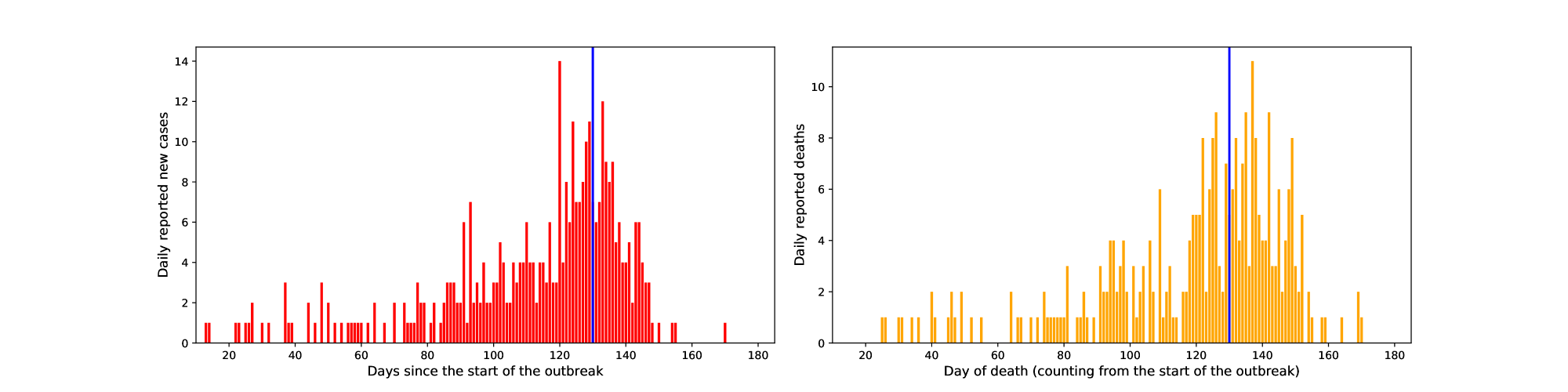
Figure 5: Synthetic data $(y_{t}^{(2,3)})_{t\geq 1}$, which are daily numbers of reported new cases, and $(y_{t}^{(3,4)})_{t\geq 1}$, which are the daily numbers of reported new deaths, simulated from the Ebola model of Lekone and Finkenstädt [2006]. Blue lines indicate the day $t_{\star}=130$ at which control measures were introduced.

Figures 6 and 7 show traceplots and histograms of the MCMC output from which the point estimates and posterior standard deviations in table 1 were calculated. The MCMC chain was run for $5\times 10^{5}$ iterations, the first $10^{5}$ iterations were discarded for burn-in, and the remaining samples thinned to result in a sample size of $10^{4}$.

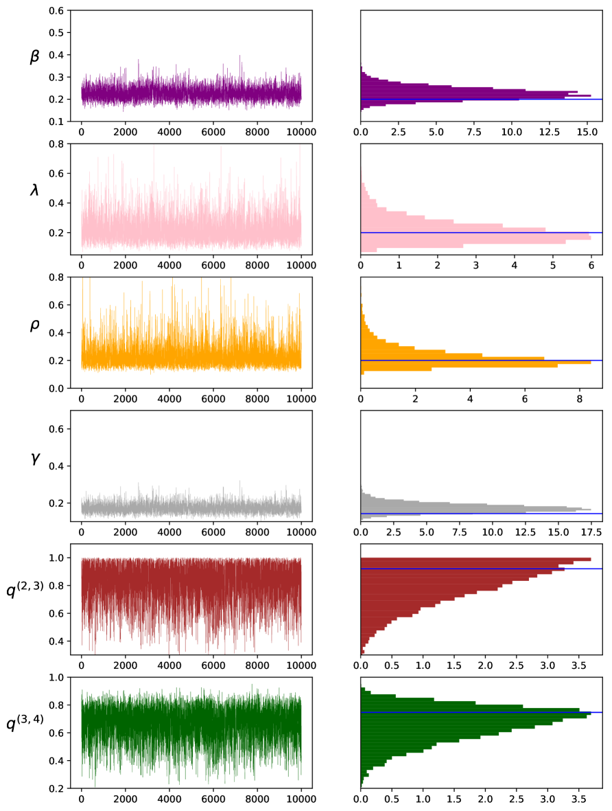
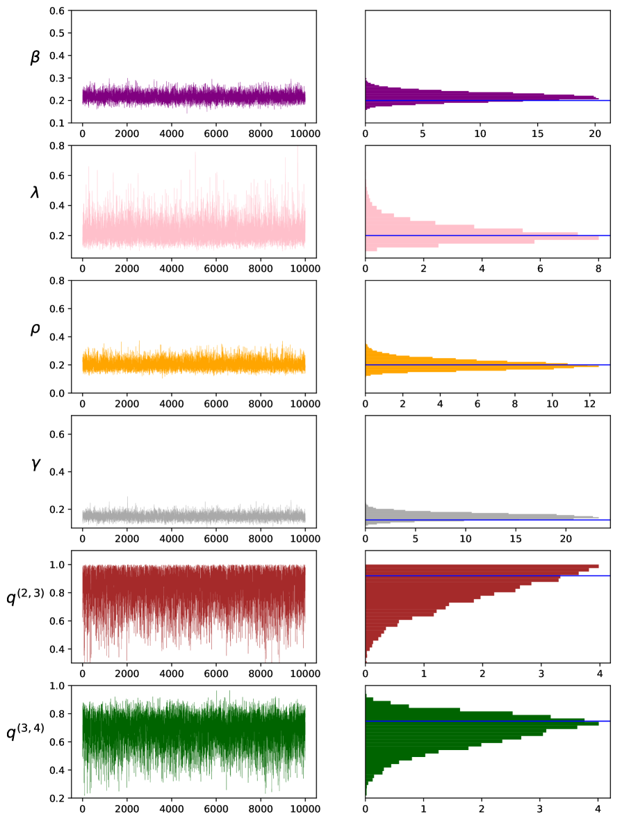
Figure 6: Traceplots and histograms for our MCMC method applied to synthetic data from the Ebola model, with the ‘vague’ set of priors (left) and the ‘informative’ set of priors (right) specified by Lekone and Finkenstädt [2006]. Blue lines show true parameter values.

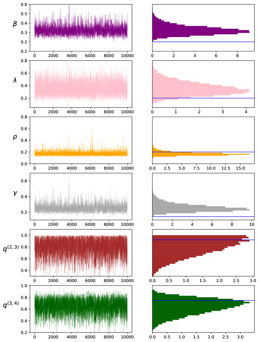
Figure 7: Traceplots and histograms for our MCMC method applied to synthetic data from the Ebola model, with the ‘noncentered’ set of priors specified by Lekone and Finkenstädt [2006]. Blue lines show true parameter values.

D.5 Real data: supplementary plots and further details for our MCMC method

The data are shown in figure 8. Traceplots and histograms for our MCMC method are displayed in figure 9, we considered only the ‘vague’ and ‘uninformative’ sets of priors.

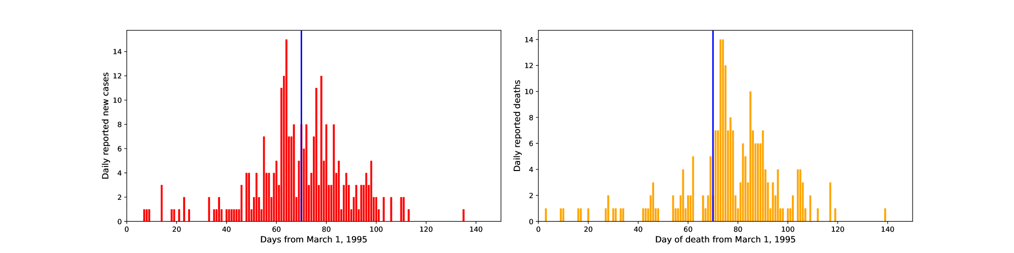
Figure 8: Data from the 1995 Ebola outbreak in the Democratic Republic of Congo per day from March 1, 1995 to July 16, 1995. Blue lines indicate the 9th of May when control measurements were introduced.

It can be observed that the posteriors over $\beta,\lambda,\rho$ appear to be bimodal under the ‘vague’ prior. According to this observation, we separated the MCMC samples out by applying the $k$-means algorithm to the marginal samples for $\rho$. Qualitatively, this identifies:

1. a mode with big $\beta$, big $\lambda$ and small $\rho$;

2. a mode with small $\beta$, small $\lambda$ and big $\rho$.

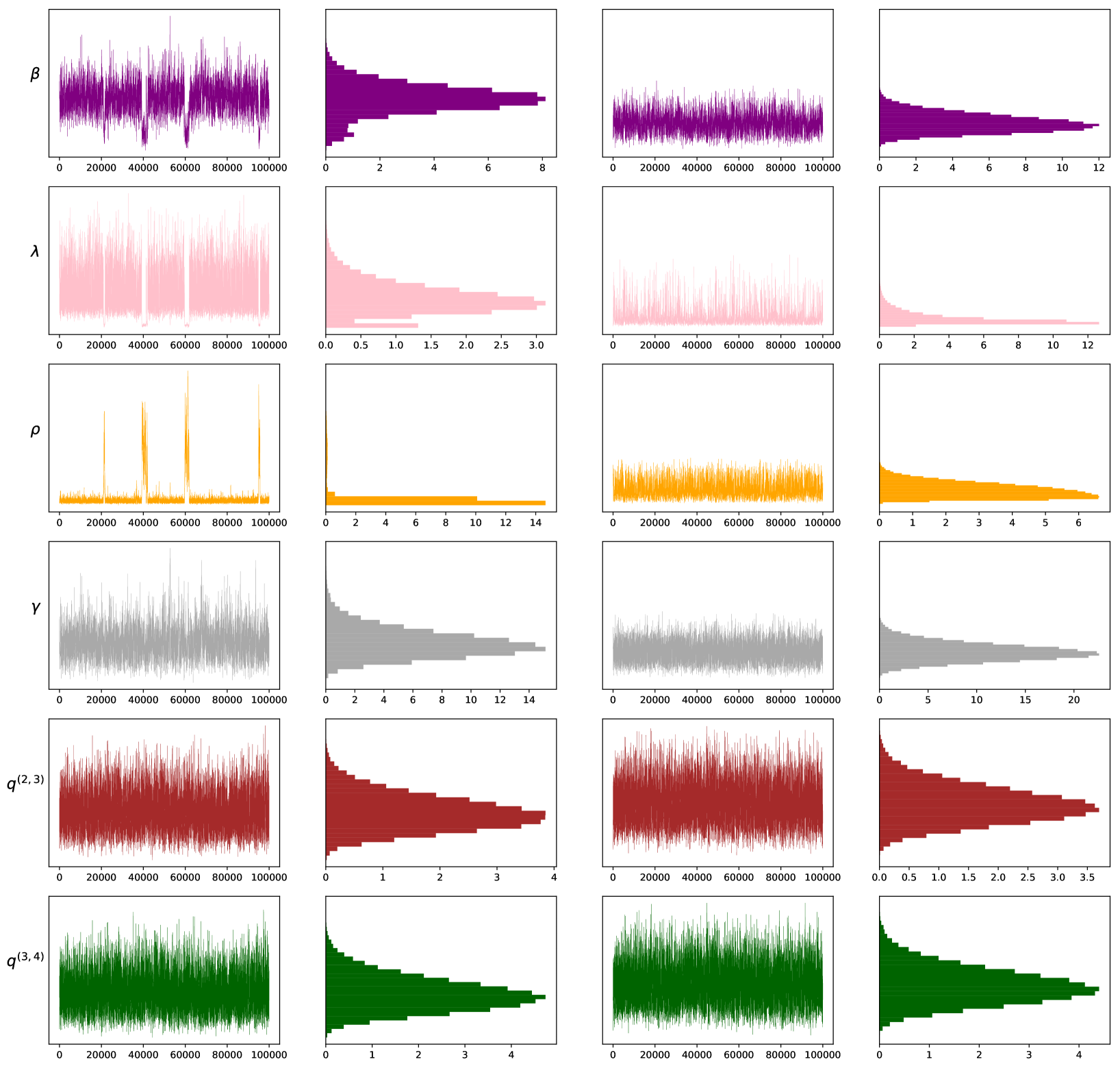
Figure 9: Traceplots and histogram for the MCMC on the Ebola data.

This can be interpreted in terms of two alternative explanations of the observed data: the first one consists of a big initial growth of the epidemic (big $\beta$) with a slow transition to the infective state (small $\rho$), followed by an effective intervention (big $\lambda$) that slows down the spread of the virus; the second one is essentially the opposite, a small initial growth of the epidemic (small $\beta$) with a fast transition to the infective state (big $\rho$), followed by mild control measures (small $\lambda$). Posterior means and standard deviations are reported in Table 2, along with the values for the Data Augmentation MCMC method of Chowell et al. [2004], and the least-squares method of Lekone and Finkenstädt [2006]. For the ABSEIR ABC method of Brown et al. [2016] we obtained the estimates ourselves by running the code available at http://grantbrown.github.io/ABSEIR/vignettes/Kikwit.html.

Observe that the estimate for $\beta$ from Lekone and Finkenstädt [2006] is close to our first mode while that from Chowell et al. [2004] is closer to our second mode. We conjecture that the analyses in these works were each exploring only a single combination of parameters and excluding the other, and we conjecture that our MCMC method mixes more quickly than that of Lekone and Finkenstädt [2006].

Appendix E COVID-19 example: further details and numerical results

E.1 Model

We consider the following discrete-time, stochastic version of the ODE model from Kucharski et al. [2020].

• $S_{t}$ is the number of susceptible individuals in Wuhan (compartment 1);

• $E^{(1,W)}_{t},E^{(2,W)}_{t}$ are the numbers of exposed individuals in Wuhan in the first and second stage of the incubation period (compartments 2&3);

• $I^{(1,W)}_{t},I^{(2,W)}_{t}$ are the numbers of infective individuals in Wuhan in the first and second stage of the disease (compartments 3&4);

• $E^{(1,T)}_{t},E^{(2,T)}_{t}$ are the numbers of individuals who were initially exposed whilst in Wuhan and subsequently travelled to other countries, in their first and second stage of the incubation period (compartments 5&6);

• $I^{(1,T)}_{t},I^{(2,T)}_{t}$ are the numbers of infective individuals who were initially exposed whilst in Wuhan and subsequently travelled to other countries, in their first and second stage of the disease (compartments 7&8);

• $R_{t}$ is the number of removed individuals (compartment 9).

The evolution of the compartments is as follows:

$$S_{t+1}=S_{t}-B^{(1,W)}_{t}-B^{(1,T)}_{t},$$ (37)

$$E^{(1,W)}_{t+1}=E^{(1,W)}_{t}+B^{(1,W)}_{t}-B^{(2,W)}_{t},$$ (38)

$$E^{(2,W)}_{t+1}=E^{(2,W)}_{t}+B^{(2,W)}_{t}-C^{(1,W)}_{t},$$ (39)

$$I^{(1,W)}_{t+1}=I^{(1,W)}_{t}+C^{(1,W)}_{t}-C^{(2,W)}_{t},$$ (40)

$$I^{(2,W)}_{t+1}=I^{(2,W)}_{t}+C^{(2,W)}_{t}-D^{W}_{t},$$ (41)

$$E^{(1,T)}_{t+1}=E^{(1,T)}_{t}+B^{(1,T)}_{t}-B^{(2,T)}_{t},$$ (42)

$$E^{(2,T)}_{t+1}=E^{(2,T)}_{t}+B^{(2,T)}_{t}-C^{(1,T)}_{t},$$ (43)

$$I^{(1,T)}_{t+1}=I^{(1,T)}_{t}+C^{(1,T)}_{t}-C^{(2,T)}_{t},$$ (44)

$$I^{(2,T)}_{t+1}=I^{(2,T)}_{t}+C^{(2,T)}_{t}-D^{T}_{t},$$ (45)

$$R_{t+1}=R_{t}+D^{(W)}_{t}+D^{(T)}_{t},$$ (46)

where:

$$\left[\begin{array}[]{c}B_{t}^{(1,W)}\\ B_{t}^{(1,T)}\\ S_{t}-B_{t}^{(1,W)}-B_{t}^{(1,T)}\end{array}\right]\sim\mathrm{Mult}\left(S_{t},\left[\begin{array}[]{c}(1-f_{t})p_{t}\\ f_{t}p_{t}\\ 1-p_{t}\end{array}\right]\right),$$

$$B^{(2,W)}_{t}\sim\mathrm{Bin}\left(E^{(1,W)}_{t},p_{C}\right),\quad B^{(2,T)}_{t}\sim\mathrm{Bin}\left(E^{(1,T)}_{t},p_{C}\right),$$ (47)

$$C^{(1,W)}_{t}\sim\mathrm{Bin}\left(E^{(2,W)}_{t},p_{C}\right),\quad C^{(1,T)}_{t}\sim\mathrm{Bin}\left(E^{(2,T)}_{t},p_{C}\right),$$ (48)

$$C^{(2,W)}_{t}\sim\mathrm{Bin}\left(I^{(1,W)}_{t},p_{R}\right),\quad C^{(2,T)}_{t}\sim\mathrm{Bin}\left(I^{(1,T)}_{t},p_{R}\right),$$ (49)

$$D^{(W)}_{t}\sim\mathrm{Bin}\left(I^{(2,W)}_{t},p_{R}\right),\quad D^{(T)}_{t}\sim\mathrm{Bin}\left(I^{(2,T)}_{t},p_{R}\right),$$ (50)

with

$$p_{t}=1-e^{-h\beta_{t}({I^{(1,W)}_{t}+I^{(2,W)}_{t}})/{n}},\quad p_{C}=1-e^{-h2\rho},\quad p_{R}=1-e^{-h2\gamma},$$ (51)

where $f_{t}$ is the fraction of cases that depart from Wuhan to other countries at time $t$. The ODE model of Kucharski et al. [2020] incorporates a a number of other compartments which are used to accumulate the numbers of individuals which have passed through certain states, but which otherwise do not play an active role in the model, hence we do not specify them here.

The time-varying transmission rate $(\beta_{t})_{t\geq 0}$ follows a log-normal random walk:

$$\beta_{t+1}=\beta_{t}\exp(V_{t}),\qquad V_{t}\sim\mathcal{N}(0,\sigma_{V}^{2}).$$

The observations consist of the new infectives in Wuhan, $y_{t}^{(3,4)}$, and internationally, $y_{t}^{(7,8)}$, at each time step, subject to random under-reporting:

$$y_{t}^{(3,4)}\sim\mathrm{Bin}\left(C_{t}^{(1,W)},q^{(W)}\right),\quad y_{t}^{(7,8)}\sim\mathrm{Bin}\left(C_{t}^{(1,T)},q^{(T)}\right).$$ (52)

E.2 Data and Parameter settings

The series $(y_{t}^{(3,4)})_{t\geq 0}$ and $(y_{t}^{(7,8)})_{t\geq 0}$, i.e. the reported numbers of new infectives in Wuhan and internationally, constitute two of the three data sets considered for inference by Kucharski et al. [2020]. They additionally considered a third data set consisting of information about prevalence of infections on evacuation flights. We exclude this prevalence data from our analysis, since the structure of the observation model required fall outside the class of models we consider in this paper.

We set $f_{t},n,\rho,\gamma$ to the same values used in Kucharski et al. [2020], including the fact that $f_{t}$ is set to zero after the date when travel restrictions were introduced. We estimated $q^{(W)}=0.00175,q^{(T)}=0.8$ via approximate maximum likelihood over a grid. We set $h=1$.

E.3 Implementation

We based our implementation directly on the R code accompanying Kucharski et al. [2020], which is available at https://github.com/adamkucharski/2020-ncov/.

We also re-ran the experiments reported in Kucharski et al. [2020] using their method, but excluding the evacuation flight data mentioned above. This allows for like-for-like comparisons of our results with theirs - see below.

E.4 Inference

Algorithm 5 Particle filter and backward sampler for COVID-19 application

1:initialize $\bm{\pi}^{(i)}_{0|0}\leftarrow\bm{\pi}_{0}$,  $\beta_{0}^{(i)}=\beta_{0},\quad\text{for }i=1,\dots,n_{\mathrm{part}}$

2:for $s=1$ to $t$ do

3:     for $i=1$ to $n_{\mathrm{part}}$ do

4:          $\beta_{s}^{(i)}\leftarrow\beta_{s-1}^{(i)}\exp(V^{(i)}),\quad V^{(i)}\sim\mathrm{N}(0,\sigma_{V}^{2})$

5:         $\mathbf{P}_{s|s-1}^{(i)}\leftarrow(\bm{\pi}^{(i)}_{s-1|s-1}\otimes\mathbf{1}_{m})\circ\mathbf{K}_{t,\bm{\pi}^{(i)}_{s-1|s-1},\beta_{t}^{(i)}}$

6:         $\mathbf{P}^{(i)}_{s|s}\leftarrow\dfrac{\mathbf{Y}_{s}}{n}+\left(1-\dfrac{\mathbf{1}_{m}^{\mathrm{T}}\mathbf{Y}_{s}\mathbf{1}_{m}}{n}\right)\dfrac{\mathbf{P}^{(i)}_{s|s-1}\circ(\mathbf{1}_{m}\otimes\mathbf{1}_{m}-\mathbf{Q}_{s})}{1-\mathbf{1}_{m}^{\mathrm{T}}(\mathbf{P}^{(i)}_{s|s-1}\circ\mathbf{Q}_{s})\mathbf{1}_{m}}$

7:         $\log w_{s}^{(i)}\leftarrow\log(n!)+\mathbf{1}_{m}^{\mathrm{T}}(\mathbf{Y}_{s}\circ\log\mathbf{P}^{(i)}_{s|s-1})\mathbf{1}_{m}+\mathbf{1}_{m}^{\mathrm{T}}(\mathbf{Y}_{s}\circ\log\mathbf{Q}_{s})\mathbf{1}_{m}-\mathbf{1}_{m}^{\mathrm{T}}\log(\mathbf{Y}_{s}!)\mathbf{1}_{m}$

8:        $+(n-\mathbf{1}_{m}^{\mathrm{T}}\mathbf{Y}_{s}\mathbf{1}_{m})\log(1-\mathbf{1}_{m}^{\mathrm{T}}(\mathbf{P}^{(i)}_{s|s-1}\circ\mathbf{Q}_{s})\mathbf{1}_{m})-\log((n-\mathbf{1}_{m}^{\mathrm{T}}\mathbf{Y}_{s}\mathbf{1}_{m})!)$

9:         $\bm{\pi}^{(p)}_{s|s}\leftarrow(\mathbf{1}_{m}^{\mathrm{T}}\mathbf{P}^{(i)}_{s|s})^{\mathrm{T}}$

10:     end for

11:     $\bar{w}_{s}^{(i)}\leftarrow w^{(s)}_{i}/\sum_{j}w^{(j)}_{s},\quad i=i,\dots,n_{\mathrm{part}}$

12:     resample $\{\beta_{s}^{(i)},\bm{\pi}^{(i)}_{s|s}\}_{i=1}^{n_{\mathrm{part}}}$ according to $\{\bar{w}^{(i)}_{s}\}_{i=1}^{n_{\mathrm{part}}}$ and keep track of ancestors in $\bm{a}_{s}=[a_{s}^{(1)}\,\cdots\,a_{s}^{(n_{\mathrm{parts}})}]^{\mathrm{T}}$

13:end for

14:

15:sample $\zeta$ according to $\{\bar{w}^{(i)}_{t}\}_{i=1}^{n_{\mathrm{part}}}$

16:$\tilde{\bm{\pi}}_{{t}|{t}}\leftarrow\bm{\pi}_{{t}|{t}}^{(\zeta)}$,  $\tilde{\mathbf{P}}_{{t}|{t}}\leftarrow\mathbf{P}_{{t}|{t}}^{(\zeta)}$,  $\tilde{\beta}_{t}\leftarrow\beta_{t}^{(\zeta)}$

17:sample $\tilde{\mathbf{Z}}_{t}$ from $\mathrm{Mult}(n,\tilde{\mathbf{P}}_{{t}|{t}})$

18:for $s=t-1,\ldots,1$ do

19:     $\tilde{\bm{\pi}}_{s|{t}}\leftarrow\tilde{\mathbf{P}}_{s+1|{t}}\mathbf{1}_{m}$

20:     $\zeta\leftarrow a_{s}^{(\zeta)}$,  $\tilde{\bm{\pi}}_{s|s}\leftarrow\bm{\pi}_{s|s}^{(\zeta)}$,  $\tilde{\mathbf{P}}_{s|s}\leftarrow\mathbf{P}_{s|s}^{(\zeta)}$,  $\tilde{\beta}_{s}\leftarrow\beta_{s}^{(\zeta)}$

21:     Let $\overline{\mathbf{L}}_{s}$ be the matrix with elements $\overline{l}_{s}^{(i,j)}\leftarrow\tilde{p}_{s|s}^{(j,i)}/\tilde{\pi}_{s|s}^{(i)}$

22:     for $i=1,\ldots,m$ do

23:         sample $\tilde{\mathbf{Z}}^{(\cdot,i)}_{s}$ from $\mathrm{Mult}((\tilde{\mathbf{Z}}_{s+1}\mathbf{1}_{m})^{(i)},\overline{\mathbf{L}}_{s}^{(i,\cdot)})$

24:     end for

25:     $\tilde{\mathbf{P}}_{s|t}\leftarrow(\mathbf{1}_{m}\otimes\tilde{\bm{\pi}}_{s|t})\circ\overline{\mathbf{L}}_{s}^{\mathrm{T}}$

26:end forreturn $\{\tilde{\beta}_{s},\tilde{\mathbf{P}}_{s|t},\tilde{\mathbf{Z}}_{s}\}_{s=1}^{t}$

Algorithm 5 is based directly on the Sequential Monte Carlo algorithm of Kucharski et al. [2020], incorporates our discrete-time stochastic model instead of their ODE model. The first stage consists of a particle filter where for time step $s$, the $i$th of $n_{\mathrm{part}}$ particles consists of $\beta_{s}^{(i)}$ and $\mathbf{P}_{s|s}^{(i)}$, and the unnormalized importance weight $w_{s}^{(i)}$ is computed similarly to algorithm 2. The second stage samples from the smoothing distribution of $\beta_{s}$ by tracing back the ancestors of a selected particle - see [Andrieu et al., 2010] for details of the role of ancestors in resampling. In addition backward steps as in algorithm 4 compute the corresponding smoothing distribution over $\mathbf{Z}_{s}$, for $s=t,\ldots,1$.

E.5 Results

The effective sample size for algorithm 5 and the SMC method of Kucharski et al. [2020] applied to the same data are reported in figure 10.

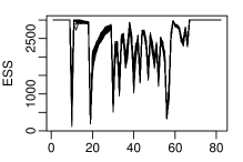
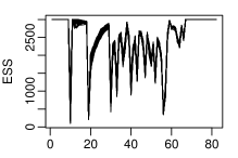
Figure 10: Effective sample size for algorithm 5 on the left, and for the the particle filter of Kucharski et al. [2020] on the right. Remark that we exclude the evacuation flights data from Kucharski et al. [2020] from the latter to make a fair comparison with our model.

We followed the procedure of Kucharski et al. [2020] in producing the remainder of our results: we ran the algorithm $100$ times with $n_{\mathrm{part}}=3\times 10^{3}$, resulting in 100 samples of $\{\tilde{\beta}_{s},\tilde{\mathbf{P}}_{s|t},\tilde{\mathbf{Z}}_{s}\}_{s=1}^{t}$ (we note that more sophisticated approaches to particle smoothing are available in the literature, but we did not use them in order to make fair comparisons with results from Kucharski et al. [2020] ). Based on these sample we then report in figure 3, in the main paper, the mean and credible intervals associated with the following 5 quantities (from Kucharski et al. [2020]). Below $\kappa$ is the rate of reporting, we used the same numerical value as in Kucharski et al. [2020], and $F^{(W)}$ and $F^{(T)}$ are auxiliary compartments.

1. The time-varying reproduction number $R_{s}=\tilde{\beta}_{s}/\gamma$ for $s=1,\dots,t$;

2. The new confirmed cases by date of onset in Wuhan and China $\tilde{y}^{(3,4)}_{s}$ for $s=1,\dots,t$:

   $$\hat{z}_{s}\sim\mathrm{Bin}\left(n,\tilde{p}^{(3,4)}_{s|t}\right)\quad\text{and}\quad\tilde{y}^{(3,4)}_{s}\sim\mathrm{Bin}\left(\hat{z}_{s},q^{(W)}\right).$$ (53)

3. The new confirmed cases by date of onset internationally $\tilde{y}^{(7,8)}_{s}$ for $s=1,\dots,t$:

   $$\hat{z}_{s}\sim\mathrm{Bin}\left(n,\tilde{p}^{(7,8)}_{s|t}\right)\quad\text{and}\quad\tilde{y}^{(7,8)}_{s}\sim\mathrm{Bin}\left(\hat{z}_{s},q^{(T)}\right).$$ (54)

4. The new confirmed cases by date in Wuhan $\Delta\widetilde{Conf}^{(W)}_{s}$ for $s=1,\dots,t$:

   $$\tilde{F}^{(W)}_{0}=0,$$ (55)

   $$\Delta\tilde{F}^{(W)}_{s}\sim\mathrm{Bin}\left(\tilde{z}_{s}^{(3,4)},1-e^{-e^{-\gamma\kappa}}\right),\quad\Delta\widetilde{Conf}^{(W)}_{s}\sim\mathrm{Bin}\left(\tilde{F}^{(W)}_{s},1-e^{-\kappa}\right),$$ (56)

   $$\tilde{F}^{(W)}_{s+1}=\tilde{F}^{(W)}_{s}+\Delta\tilde{F}^{(W)}_{s}-\Delta\widetilde{Conf}^{(W)}_{s}.$$ (57)

5. The new confirmed cases by date internationally $\Delta\widetilde{Conf}^{(T)}_{s}$ for $s=1,\dots,t$:

   $$\tilde{F}^{(T)}_{0}=0,$$ (58)

   $$\Delta\tilde{F}^{(T)}_{s}\sim\mathrm{Bin}\left(\tilde{z}_{s}^{(7,8)},1-e^{-e^{-\gamma\kappa}}\right),\quad\Delta\widetilde{Conf}^{(T)}_{s}\sim\mathrm{Bin}\left(\tilde{F}^{(T)}_{s},1-e^{-\kappa}\right),$$ (59)

   $$\tilde{F}^{(T)}_{s+1}=\tilde{F}^{(T)}_{s}+\Delta\tilde{F}^{(T)}_{s}-\Delta\widetilde{Conf}^{(T)}_{s}.$$ (60)

Figure 11 shows the results for the SMC algorithm Kucharski et al. [2020] applied to the same data as our method, i.e. with the evacuation flights data left out of the analysis. Therefore figure 11 can be compared directly against our figure 3 - see discussion in the main part of the paper.

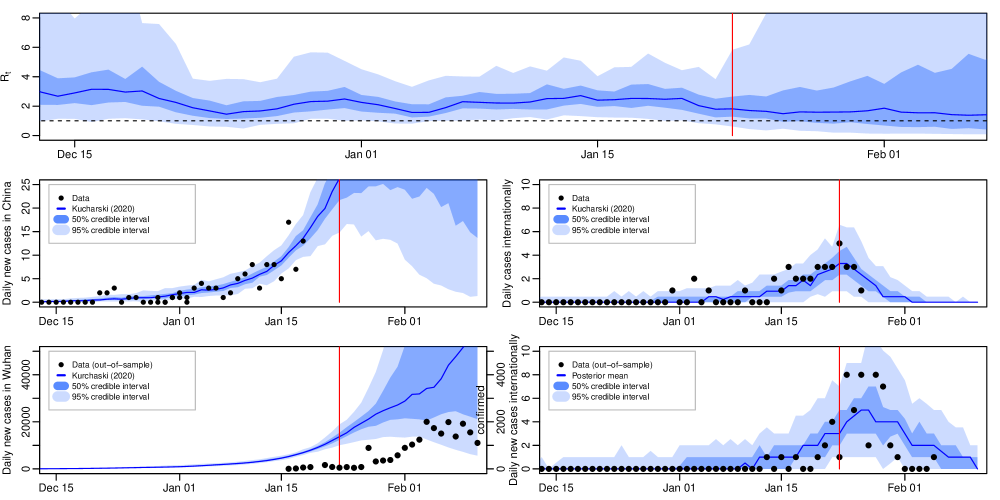
Figure 11: Results for the COVID-19 model using Kucharski et al. [2020] methods without rescue flights data. Red line is date at which travel restrictions were introduced. Top: estimated reproduction number. Middle row: estimated daily new confirmed cases in Wuhan (left) and internationally (right), both with in-sample data by date of symptom onset. Bottom row, left: estimated new symptomatic but possibly unconfirmed cases (left axis) and out-of-sample new confirmed cases data (right axis); right: estimated confirmed international cases by date of confirmation, and out-of-sample data.

References

- Andrieu et al. (2010) Christophe Andrieu, Arnaud Doucet, and Roman Holenstein. Particle markov chain monte carlo methods. Journal of the Royal Statistical Society: Series B (Statistical Methodology), 72(3):269–342, 2010.
- Brauer (2008) Fred Brauer. Compartmental models in epidemiology. Springer, 2008.
- Bretó (2018) Carles Bretó. Modeling and inference for infectious disease dynamics: a likelihood-based approach. Statistical Science: a review journal of the Institute of Mathematical Statistics, 33(1):57–69, 2018.
- Briers et al. (2010) Mark Briers, Arnaud Doucet, and Simon Maskell. Smoothing algorithms for state–space models. Annals of the Institute of Statistical Mathematics, 62(1):61, 2010.
- Brown et al. (2016) Grant D Brown, Jacob J Oleson, and Aaron T Porter. An empirically adjusted approach to reproductive number estimation for stochastic compartmental models: A case study of two Ebola outbreaks. Biometrics, 72(2):335–343, 2016.
- Brown et al. (2018) Grant D Brown, Aaron T Porter, Jacob J Oleson, and Jessica A Hinman. Approximate Bayesian Computation for spatial SEIR(S) epidemic models. Spatial and Spatio-temporal Epidemiology, 24:27–37, 2018.
- Cappé et al. (2006) Olivier Cappé, Eric Moulines, and Tobias Rydén. Inference in hidden Markov models. Springer Science & Business Media, 2006.
- Chowell et al. (2004) Gerardo Chowell, Nick W Hengartner, Carlos Castillo-Chavez, Paul W Fenimore, and Jim Michael Hyman. The basic reproductive number of Ebola and the effects of public health measures: the cases of Congo and Uganda. Journal of Theoretical Biology, 229(1):119–126, 2004.
- de Lusignan et al. (2020) Simon de Lusignan, Jamie Lopez Bernal, Maria Zambon, Oluwafunmi Akinyemi, Gayatri Amirthalingam, Nick Andrews, Ray Borrow, Rachel Byford, André Charlett, Gavin Dabrera, et al. Emergence of a novel coronavirus (COVID-19): protocol for extending surveillance used by the Royal College of general practitioners research and surveillance centre and public health England. JMIR Public Health and Surveillance, 6(2):e18606, 2020.
- Farach-Colton and Tsai (2015) Martín Farach-Colton and Meng-Tsung Tsai. Exact sublinear binomial sampling. Algorithmica, 73(4):637–651, 2015.
- Fasiolo et al. (2016) Matteo Fasiolo, Natalya Pya, and Simon N Wood. A comparison of inferential methods for highly nonlinear state space models in ecology and epidemiology. Statistical Science, 31(1):96–118, 2016.
- Funk and King (2020) Sebastian Funk and Aaron A King. Choices and trade-offs in inference with infectious disease models. Epidemics, 30:100383, 2020.
- Gelman et al. (1996) Andrew Gelman, Xiao-Li Meng, and Hal Stern. Posterior predictive assessment of model fitness via realized discrepancies. Statistica Sinica, 6(4):733–760, 1996.
- Kucharski et al. (2020) Adam J Kucharski, Timothy W Russell, Charlie Diamond, Yang Liu, John Edmunds, Sebastian Funk, Rosalind M Eggo, Fiona Sun, Mark Jit, James D Munday, et al. Early dynamics of transmission and control of COVID-19: a mathematical modelling study. The Lancet Infectious Diseases, 20(5):553–558, 2020.
- Kurtz (1970) Thomas G Kurtz. Solutions of ordinary differential equations as limits of pure jump Markov processes. Journal of Applied Probability, 7(1):49–58, 1970.
- Kurtz (1971) Thomas G Kurtz. Limit theorems for sequences of jump Markov processes approximating ordinary differential processes. Journal of Applied Probability, 8(2):344–356, 1971.
- Kypraios et al. (2017) Theodore Kypraios, Peter Neal, and Dennis Prangle. A tutorial introduction to Bayesian inference for stochastic epidemic models using Approximate Bayesian Computation. Mathematical Biosciences, 287:42–53, 2017.