Resonances in pulsatile channel flow with an elastic wall

Abstract

Interactions between fluids and elastic solids are ubiquitous in application ranging from aeronautical and civil engineering to physiological flows. Here we study the pulsatile flow through a two-dimensional Starling resistor as a simple model for unsteady flow in elastic vessels. We numerically solve the equations governing the flow and the large-displacement elasticity and show that the system responds as a forced harmonic oscillator with non-conventional damping. We derive an analytical prediction for the amplitude of the oscillatory wall deformation, and thus the conditions under which resonances occur or vanish.

Flow-induced pressure fluctuations acting on elastic structures can excite large-amplitude oscillations – the most famous example being the catastrophic failure of the Tacoma-Narrows bridge Billah and Scanlan (1991). In physiology, fluid-structure interaction is associated with cardiovascular disease Ku (1997), but it also helps regulate the blood supply to internal organs Shapiro (1977) and return blood to the heart during diastole Casey and Hart (2008). Physiological flows are extremely complex and feature a large variability across individuals, which prevents accurate predictions even with state-of-the-art computational methods Valen-Sendstad et al. (2018). Therefore there has been a desire to study the key physical mechanisms in simpler setups Heil and Hazel (2011). The Starling resistor Knowlton and Starling (1912); Conrad (1969) is a canonical system that has been widely used to investigate the nonlinearly coupled dynamics of fluid flow and the deformation of elastic vessels. The setup consists of an elastic tube mounted between two rigid pipes in a pressurized chamber (or its two-dimensional analogue, the collapsible channel shown in Fig. 1).

In Starling resistors the flow is typically driven by a constant pressure drop between inlet and outlet. For this case, rich nonlinear phenomena, such as flow limitation Kamm and Shapiro (1979) and self-excited oscillations Conrad (1969); Jensen and Heil (2003); Bertram (2008); Stewart et al. (2009), have been observed. By contrast, studies of pulsatile flows through elastic tubes and channels Conrad (1969); Low and Chew (1991); Tubaldi et al. (2016); Tsigklifis and Lucey (2017); Stelios et al. (2019); Amabili et al. (2020a) are comparatively scarce despite the pulsatile nature of blood flows. A notable exception is Amabili et al.’s recent study Amabili et al. (2020b) in which part of an excised human aorta was mounted between two rigid pipes and subjected to physiological pulsatile pressure and flow rates.

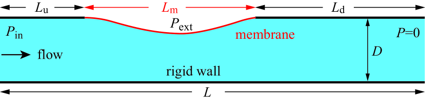
Figure 1: (Color online) Sketch of fluid flow in a collapsible channel. A pulsatile pressure $P_{\text{in}}$ of mean $P_{0}$ and frequency $\Omega$ drives fluid of kinematic viscosity $\nu$ and density $\rho$ through a channel of total length $L$ and width $D$. The lower channel wall is rigid, whereas a pre-stressed, elastic membrane of length $L_{\text{m}}$ is clamped between two rigid segments at the upper wall and is pressurized by an external pressure $P_{\text{ext}}$. The upstream and downstream segments have lengths $L_{\text{u}}$ and $L_{\text{d}}$, respectively.

In this Letter we show that pulsatile flow in a two-dimensional collapsible channel exhibits strong resonances, reminiscent of a forced damped harmonic oscillator. Guided by this observation, we develop a simple mathematical model which successfully predicts the resonances, the phase lag between the amplitude and the imposed pressure, and also the conditions under which resonances vanish.

We consider a fluid of kinematic viscosity $\nu$ and density $\rho$, whose motion is governed by the incompressible Navier–Stokes equations

$$\dfrac{\partial{\bf u}}{\partial t}+{\bf u}\cdot\nabla{\bf u}=-\nabla p+\nabla^{2}{\bf u},\quad\nabla\cdot{\bf u}=0.$$ (1)

Here and elsewhere all lengths are scaled on the channel height, $D$, and time, $t$, on the timescale for viscous diffusion, $D^{2}/\nu$. The fluid velocity ${\bf u}$ is non-dimensionalized on $\nu/D$ and the pressure, $p$, on $\rho\nu^{2}/D^{2}$. We set the pressure at the downstream end of the channel to zero and drive the flow by setting the dimensionless pressure at the upstream end to

$$p=p_{\rm in}(t)=12\mathit{Re}\,l\left(1+A\sin\,(\alpha^{2}\,t)\right),$$ (2)

where $l=L/D$. The dimensionless forcing frequency $\alpha^{2}=\Omega D^{2}/\nu$ ($\Omega$ is the dimensional frequency and $\alpha$ the Womersley number) characterizes the ratio of the timescale for viscous diffusion to the period of the imposed pressure pulsation; $A$ is the amplitude of the oscillatory component of the pressure relative to the steady one. The Reynolds number $\mathit{Re}=D{\cal U}/\nu$ is defined with the mean speed of the Poiseuille flow generated by a steady pressure drop $P_{0}$ in the undeformed channel, ${\cal U}=P_{0}D^{2}/(12\rho\nu L)$. The boundary conditions for the velocity are no-slip on the walls, and parallel flow is assumed at the inflow and outflow boundaries.

We model the elastic segment of the wall as a thin, massless membrane (of dimensional thickness $\mathfrak{h}$ and Young’s modulus $E$, subject to a dimensional pre-stress $\Sigma_{0}$) which deforms in response to the combined effects of the external pressure and the fluid stresses. The resulting traction vector acting on the membrane, non-dimensionalized on the pre-stress $\Sigma_{0}$, is given by

$${\bf f}=-p_{\text{ext}}{\bf n}+\frac{1}{T}\left[p{\bf n}-\left(\nabla{\bf u}+(\nabla{\bf u})^{\rm T}\right)\cdot{\bf n}\right],$$ (3)

where ${\bf n}$ is the outer normal to the membrane, $p_{\text{ext}}=P_{\text{ext}}/\Sigma_{0}$ and the superscript ^T denotes the transpose of a matrix. The parameter $T=\Sigma_{0}\,D^{2}/(\rho\nu^{2})$ represents the ratio of the pre-stress to the fluid pressure and is a measure of the tension in the bounding membrane. We parametrize the shape of the membrane by a dimensionless Lagrangian coordinate $\xi$ so that the position vector to a material point in the membrane is given by ${\bf R}(\xi,t)={\bf r}(\xi)+{\bf d}(\xi,t)$. Here ${\bf r}(\xi)=[\xi,1]^{\rm T}$ defines the undeformed configuration and ${\bf d}(\xi,t)$ is the displacement vector. The membrane deformation is governed by the principle of virtual displacements

$$\int_{0}^{l_{\text{m}}}\left((\sigma_{0}+\gamma)\delta\gamma+\frac{1}{12}h^{2}\kappa\,\delta\kappa-\frac{\sigma_{0}\Lambda}{h}\ {\bf f}\cdot\delta{\bf R}\right)d\xi=0,$$ (4)

where $h=\mathfrak{h}/D$ is the dimensionless thickness of the membrane, $\sigma_{0}=\Sigma_{0}/E$ the dimensionless pre-stress, $\gamma=\partial d_{x}/\partial{\xi}+\frac{1}{2}[(\partial d_{x}/\partial{\xi})^{2}+(\partial d_{y}/\partial{\xi})^{2}]$ is a measure of the extensional strain, and $\kappa=[(\partial^{2}d_{y}/\partial{\xi^{2}})(1+\partial d_{x}/\partial{\xi})-(\partial^{2}d_{y}/\partial{{\xi}^{2}})(\partial d_{y}/\partial{\xi})]/\Lambda$ provides a measure of the bending deformation, with $\Lambda=[(1+\partial d_{x}/\partial\xi)^{2}+(\partial d_{y}/\partial{\xi})^{2}]^{1/2}$. Both measures are fully geometrically nonlinear. The only linearization occurs in the assumption of incrementally linear Hookean behavior in the constitutive equation, which is based on the assumption that the pre-stress is much larger than the stresses induced by the actual deformation, $\sigma_{0}\gg 1$.

We solved the time-dependent fully-coupled fluid-structure interaction problem with the open-source library oomph-lib Heil and Hazel (2006). All simulations shown here were performed with $A=1$, $h=0.01$, $l_{\text{m}}=L_{\text{m}}/D=10$, $l_{\text{u}}=L_{\rm u}/D=5$ and $l_{\text{d}}=L_{\text{d}}/D=10$.

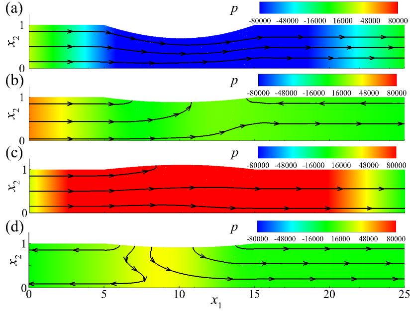
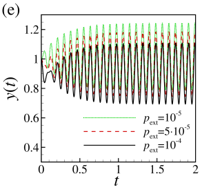
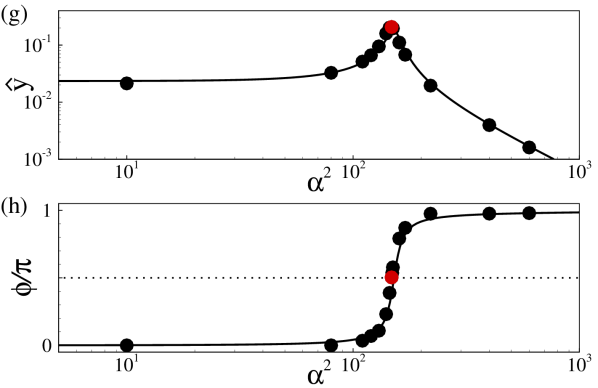
Figure 2: (Color online) (a)-(d) Pressure contours and streamlines at four equally-spaced instants throughout the period of the oscillation for $\alpha^{2}=148$, $\mathit{Re}=100$, $\sigma_{0}=10^{3}$, $T=10^{9}$ and $p_{\text{ext}}=10^{-4}$ after the decay of the initial transients. (e) Time trace of the vertical displacement of the membrane mid-point, $y(t)$, at the same parameters as (a-d) except for three different external pressures ($p_{\text{ext}}=10^{-5}$, $5\cdot 10^{-5}$ and $10^{-4}$). (f) The same data of (e) after subtracting the time-averaged displacements, $\overline{y}$, following the decay of the initial transients ($\overline{y}=1.017,0.965,0.900$, respectively). (g) The oscillation amplitude and (h) the corresponding phase lag between response and forcing as a function of $\alpha^{2}$, where the red dots mark the case for (a)–(d) and the horizontal dotted line marks $\phi=\pi/2$. All other parameters are as in (a)–(d).

We started the simulations from an initial condition in which the membrane is undeformed and the velocity field is steady Poiseuille flow. Following the decay of initial transients the system settles into a time-periodic motion with the period of the forcing, $2\pi/\alpha^{2}$. The snapshots in Figs. 2(a-d) show that the inward wall motion displaces a significant amount of fluid from the central region of the channel and thus creates strong sloshing flows which are superimposed on the pressure-driven pulsatile flow. These are reminiscent of the flows observed in a study of self-excited oscillations in collapsible channels Jensen and Heil (2003).

We characterize the dynamics of the system by monitoring the vertical displacement of the membrane at its midpoint, $y(t)$. Fig. 2(e) shows time traces of this quantity for a range of external pressures. In Fig. 2(f) we plot the same data but subtract the time-average displacement $\overline{y}$ following the decay of the initial transients (whose duration is of the order of the viscous time unit, $D^{2}/\nu$). We observe that the amplitude of the steady-state oscillations, $\widehat{y}$, is approximately independent of the external pressure (and from now on we set $p_{\text{ext}}=10^{-4}$). Fig. 2(g) shows that the amplitude of the oscillations, $\widehat{y}$, exhibits a sharp maximum at a specific forcing frequency, $\alpha^{2}_{\rm max}$. Furthermore, the phase lag $\phi$ between the displacement $y(t)$ and the forcing pressure $p_{\rm in}(t)$ displays a $90^{\circ}$ phase shift when the amplitude reaches its maximum; see Fig. 2(h).

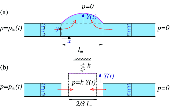
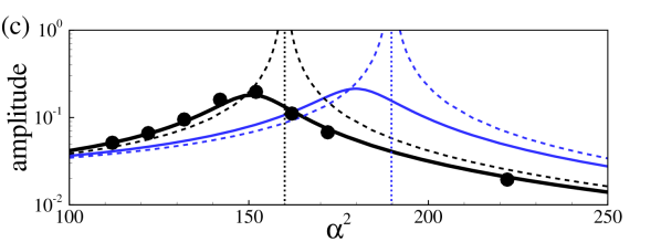
Figure 3: (Color online) (a)–(b) Sketch of the model. (c) Oscillation amplitude against $\alpha^{2}$ from the model at $Re=100$, $\sigma_{0}=10^{3}$, $T=10^{9}$, where the solid and the dashed lines denote the viscous and the inviscid prediction, and black and blue correspond to $\beta=0.25$ and $\beta=0$. The black symbols show the results from the simulations (as in Fig. 2(g), with some symbols omitted for clarity). The dotted lines mark the corresponding eigenfrequencies.

To elucidate the mechanism responsible for this behavior we will now develop a simple theoretical model that describes the response of the collapsible channel to the imposed pressure pulsations at its upstream end. Since we found the external pressure to have little effect on the system’s behavior, we set it to zero and thus consider the setup sketched in Fig. 3(a). We assume the upstream and downstream rigid parts of the channel to be sufficiently long, $l_{\rm u},l_{\rm d}\gg 1$, so that in these segments the horizontal component of the velocity, $u$, is much larger than its vertical counterpart. Our computations show that this assumption is appropriate even in the relatively short channels used in our simulations; see Fig. 2(a)–(d). The horizontal component of the momentum equation (1) can then be approximated by

$$\frac{\partial u}{\partial t}=-\frac{\partial p}{\partial x}+\frac{\partial^{2}u}{\partial y^{2}},$$ (5)

where the pressure gradient only depends on time, $\partial p/\partial x=G(t)$, and we have $u=u(y,t)$. We assume that the vertical displacement of the elastic membrane can be described by the product of a mode shape $M(x)$ and an amplitude $Y(t)$, so that

$$y_{\rm m}(x,t)=1+Y(t)\,M(x).$$ (6)

Based on the shapes observed in the computations, we approximate $M(x)$ by a quadratic function, $M(x)=4(x/l_{\rm m})(1-(x/l_{\rm m}))$. Given that the elastic membrane is under a large, approximately constant tension we describe its deformation by Laplace’s law, implying that the fluid pressure in the elastic segment is given by the product of the membrane curvature and its tension. For the assumed mode shape the dimensionless fluid pressure under the membrane is $p_{\rm m}=k\,Y(t),$ where $k=8\,h\,T/l_{\rm m}^{2}$. By exploiting that the flows in the two rigid segments are fully developed and coupled by mass conservation, we show in the Supplementary Material that the displacement of the membrane $Y$ obeys the following equation

$$\frac{2}{3}l_{\rm m}\frac{{\rm d}^{2}Y}{{\rm d}t^{2}}+k\frac{l_{\rm u}+l_{\rm d}}{l_{\rm u}l_{\rm d}}\ Y+\left.\left(\frac{\partial u_{\rm d}}{\partial y}-\frac{\partial u_{\rm u}}{\partial y}\right)\right|_{y=0}^{1}=\frac{p_{\rm in}(t)}{l_{\rm u}}.$$ (7)

This equation can be interpreted in terms of the difference in the pressure gradients in the upstream and downstream segments driving an acceleration in the net flow away from the centre, which must be balanced by the change in volume of the elastic section, see eq. (S13) in the Supplementary Material.

The last term on the left hand side of eq. (7) arises from the viscous terms in the momentum equation and represents the effect of the viscous shear stresses acting on the walls of the rigid segments. The remaining terms show that in the absence of viscous damping the system is a forced linear oscillator with natural frequency

$$\alpha_{\rm eig}^{2}=\left(\frac{3}{2}\frac{k}{l_{\rm m}}\frac{l_{\rm u}+l_{\rm d}}{l_{\rm u}l_{\rm d}}\right)^{1/2}=\left(\frac{12\,h\,T(l_{\rm u}+l_{\rm d})}{l_{\rm m}^{3}l_{\rm u}l_{\rm d}}\right)^{1/2}.$$ (8)

The damping term in equation (7) is more complicated than in a standard harmonic oscillator (see the Supplementary Material).

Our model equation (7) therefore predicts that the collapsible channel behaves like the linear oscillator sketched in Fig. 3(b): The elastic membrane of length $l_{\rm m}$ is equivalent to a piston of width $\frac{2}{3}l_{\rm m}$, mounted on a spring of stiffness $k$. The piston is displaced by the net influx of fluid from the rigid segments and sets the fluid pressure acting at their internal boundaries. The system’s oscillations are governed by a dynamic balance between fluid inertia and the elastic restoring forces, with the fluid viscosity providing damping.

The amplitude $|\widehat{Y}|$ of the time-harmonic solutions, $Y(t)=\widehat{Y}\exp({\rm i}\alpha^{2}t)$, to (7) is given in the Supplementary Material, eq. (S11). The blue solid line in Fig. 3(c) shows a plot of the theoretically predicted amplitude as a function of the forcing frequency $\alpha^{2}$ for the same parameters as in Fig. 2(g). The thin blue dashed line shows the corresponding inviscid response, with the natural frequency $\alpha^{2}_{\rm eig}$ shown by the blue vertical dotted line. Viscous effects eliminate the unbounded response of the inviscid system at $\alpha^{2}=\alpha^{2}_{\rm eig}$ and reduce the resonant frequency. The theoretical predictions are in good qualitative agreement with the computational results, but they over-estimate the resonant frequency. This is a consequence of us having neglected the dynamics of the fluid that moves within the elastic segment itself. We can include this effect by replacing $l_{\rm u/d}$ by corresponding effective lengths $l_{\rm u/d}^{\rm[eff]}=l_{\rm u/d}+\beta l_{\rm m}$, where the parameter $\beta$ represents the fraction of the fluid in the elastic segment that participates in the oscillatory (sloshing) motion. The black lines in Fig. 3(c) show the theoretical predictions for $\beta=1/4$. This value produces near-perfect agreement with the results of the simulations for all the cases considered (see Table S1 in the Supplementary Material for a full list of all computations) and is kept fixed hereinafter.

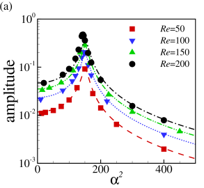
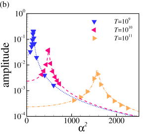
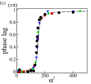
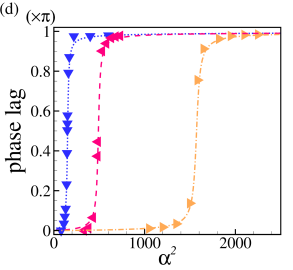
Figure 4: (Color online) (a) Oscillation amplitude against $\alpha^{2}$ for $\sigma_{0}=10^{3}$ and $T=10^{9}$ for four Reynolds numbers, and the corresponding phase lag (c). (b) Oscillation amplitude against $\alpha^{2}$ for $Re=100$, $\sigma_{0}=10^{3}$ and three values of $T$, and the corresponding phase lag (d). The symbols and the lines denote the simulation and the model predictions, respectively.

We note that the theoretical model predicts the system’s response to be controlled by the parameter $T$ and the geometry; the Reynolds number $Re$ is predicted to affect only the amplitude of the response, but not the resonant frequency. Fig. 4 shows the amplitude (top row) and phase (bottom row) as a function of the forcing frequency $\alpha^{2}$ for a constant value of $T$ (left) and a constant value of $Re$ (right). The agreement between the theoretical predictions and computational results is remarkable, even for oscillations of large amplitude (Fig. 4 includes cases where the amplitude reaches values as large as 48% of the channel width). The amplitude increases proportionally to the Reynolds number. A reduction in the membrane tension ($T$) increases the amplitude of the oscillation and reduces the resonant frequency. This suggests that for sufficiently small values of $T$ the maximum amplitude may occur in the quasi-steady limit ($\alpha^{2}\to 0$). However, for the parameter values of Fig. 4 this happens when the theoretically predicted amplitude exceeds the undeformed channel width, i.e. $|\widehat{Y}|>1$, rendering the theoretical model inapplicable. To explore the disappearance of the resonance at smaller values of $T$ we therefore reduced the Reynolds number significantly.

Fig. 5(a) shows a plot of the amplitude as a function of the forcing frequency $\alpha^{2}$ for three values of $T$ and for a Reynolds number of $Re=0.25$. For $T=10^{8}$ there is a clearly defined resonance at $\alpha_{\rm max}^{2}\approx 45$; a reduction of $T$ to $10^{7}$ increases the maximum amplitude but weakens the resonance and moves it to smaller values of the forcing frequency, $\alpha_{\rm max}^{2}\approx 12.5$; finally, for $T=10^{6}$ the maximum amplitude is obtained in the quasi-steady limit, implying the disappearance of the resonance.

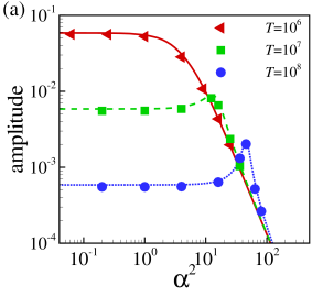
Figure 5: (Color online) (a) Oscillation amplitude against frequency $\alpha^{2}$ at $Re=0.25$, $\sigma_{0}=10^{3}$. The maximum oscillation amplitude for $T=10^{8}$ and $10^{7}$ occurs at $\alpha^{2}\approx 45$ and $12.5$, respectively, and at $T=10^{6}$ the maximum amplitude is approached as $\alpha^{2}\to 0$. The symbols and the lines denote the simulation and the model, respectively. (b) The frequency $\alpha^{2}_{\text{max}}$ as a function of $T$. The symbols denote $\alpha^{2}_{\text{max}}$ from the simulation. The red solid line and the black dashed line denote the model predictions of $\alpha^{2}_{\text{eig}}$ and $\alpha^{2}_{\text{max}}$, respectively. The parameters used in the simulations are listed in table S1 in the Supplementary Material.

Fig. 5(b) shows how the natural frequency, $\alpha^{2}_{\rm eig}$, and the frequency, $\alpha^{2}_{\rm max}$, at which the system has its maximum response, depend on the system parameters. For large values of $T$ the maximum response occurs close to the natural frequency, $\alpha^{2}_{\rm max}\lesssim\alpha^{2}_{\rm eig}$, and both scale with the square root of $T$ as suggested by equation (8). Just below $T\approx 2\times 10^{6}$ the resonance disappears. Finally, we probed the dependence of the system’s response on the geometry by performing simulations for various combinations of $l_{\rm m}$, $l_{\rm u}$, $l_{\rm d}$ and $h$. As shown in Fig. S1 in the Supplementary Material, the scaling suggested by the inviscid approximation (8) leads to a near-perfect collapse of all the results onto a single master curve ($\beta=0.25$ was kept fixed).

In summary, the response of a collapsible channel is described by a harmonic oscillator with non-standard damping, even in regimes where the imposed pulsations in fluid pressure induce very large wall deflections. Our model accurately predicts the response of the system as a function of the ten independent parameters that govern it ($l_{\rm m}$, $l_{\rm u}$, $l_{\rm d}$, $h$, $p_{\text{ext}}$, $Re$, $A$, $\alpha^{2}$, $T$ and $\sigma_{0}$). The tension and the dimensions of the channel segments solely determine the system’s natural frequency, whereas the amplitude of the response also depends on the frequency and amplitude of the pressure pulsations (the latter is set by $A\,Re$, see Fig. S2 in the Supplementary Material). While our simulations were performed for a 2D system the mechanism can be generalized to a 3D setting. The characterization of oscillations during which the elastic tube undergoes an axisymmetric inflation is straightforward, whereas the characterization of non-axisymmetric oscillations could benefit from a ‘tube-law’-based description Whittaker et al. (2010).