Equivalence in Deep Neural Networks via Conjugate Matrix Ensembles

Abstract

A numerical approach is developed for detecting the equivalence of deep learning architectures. The method is based on generating Mixed Matrix Ensembles (MMEs) out of deep neural network weight matrices and conjugate circular ensemble matching the neural architecture topology. Following this, the empirical evidence supports the phenomenon that difference between spectral densities of neural architectures and corresponding conjugate circular ensemble are vanishing with different decay rates at the long positive tail part of the spectrum i.e., cumulative Circular Spectral Difference (CSD). This finding can be used in establishing equivalences among different neural architectures via analysis of fluctuations in CSD. We investigated this phenomenon for a wide range of deep learning vision architectures and with circular ensembles originating from statistical quantum mechanics. Practical implications of the proposed method for artificial and natural neural architectures discussed such as the possibility of using the approach in Neural Architecture Search (NAS) and classification of biological neural networks.

I Introduction

Constructing equivalence relations among different mathematical structures are probably one of the most foundational concepts in sciences Rosser (2008), a practical interest as well, beyond being a theoretical building block of many quantitative fields. This manifests in many fields of physical sciences and in practice, such as for equivalence of graph network ensembles Barré and Gonçalves (2007); den Hollander et al. (2018), single-molecule experiments Costeniuc et al. (2005); Süzen et al. (2009), Bayesian Networks Chickering (2002), between ranking algorithms Ertekin and Rudin (2011) and Brain network motifs Sporns and Kötter (2004); Bullmore and Sporns (2009).

Recent success of deep learning Schmidhuber (2015); LeCun et al. (2015) in different learning tasks showing skills exceeding human capacity, specially in vision tasks brings the need for both understanding of these systems and build neural architectures in an efficient manner. In this direction, detecting equivalent deep learning architecures are not only interesting for theoretical understanding but also for finding more efficient architecture as a design principle. Neural Architecture Search (NAS) Elsken et al. (2019); Ren et al. (2020) or search for smaller equivelent network, i.e., architecture compression Kumar et al. (2019); Serra et al. (2020) are valuable tools in achieving this aim.

Approach in establishing equivalence between two deep learning architectures are taken here lies in the analysis of eigenvalue spectra of the trained weights, network topology and generating conjugate random matrix ensemble. There will be no dependence on the activation functions or training procedure in establishing such equivalance. This makes proposed approach appealing as it can be applied to wide-variety of network setting and learning procedures. However, the equivalence would capture components of topological structure, learning procedure and network setting. This sort of analysis can be considered as gaining understanding of structure and function relationships and stems from topological data analysis Bubenik (2015); Cang and Wei (2017); Rieck et al. (2018); Wasserman (2018).

The analysis of spectral density of weights of deep learning architectures recently investigated Pennington et al. (2018); Sagun et al. (2017); Rieck et al. (2018); Martin and Mahoney (2019); Süzen et al. (2019). We follow a similar ethos in this regard, as earlier work is pioneered such analysis on investigating eigenvalue statistcs in neural network learning Le Cun et al. (1991).

II Mixed matrix ensembles

In establishing equivalence of two neural networks, we have taking a route that requires a mathematical setting in the language of matrix ensembles, square matrices. Matrix ensembles especially appear in random matrix theory Mehta (2004); Wigner (1967). One of the prominent example is circular complex matrix ensembles Dyson (1962) that mimics quantum statistical mechanics systems Haake (2013). It is hinted out that decay of spectral ergodicity with increasing matrix order $N$ for circular matrix ensembles signifies an analogous behaviour as using deeper layers in neural networks Süzen et al. (2017), whereby circular ensembles used as a simulation tool. However, real deep learning architectures have rarely all the same order weight matrices, but the weight matrices extracted from trained deep learning architectures will have variety of different orders due to different units in layer connections and forms a Layer Matrix Ensemble, see Definition 1.

Definition 1.

Layer Matrix Ensemble $\mathscr{L}^{m}$ Süzen et al. (2019) The weights $W_{l}\in\mathbb{R}^{p_{1}\times p_{2}\times...\times p_{n}}$ are obtained from a trained deep neural network architecture’s layer $l$ as an $n$-dimensional Tensor. A Layer Matrix Ensemble $\mathscr{L}^{m}$ is formed by transforming $m$ set of weights $W_{l}$ to square matrices $X_{l}\in\mathbb{R}^{N_{l}\times N_{l}}$, that $X_{l}=A_{l}\cdot A_{l}^{T}$ and $A_{l}\in\mathbb{R}^{N_{l}\times M_{l}}$ is marely a stacked up version (projecting an arbitrary tensor to a matrix) of $W_{l}$ where $n>1$, $N_{l}=p_{1}$, $M_{l}=\prod_{j=2}^{n}p_{j}$ and $p_{j},n,m,N_{l},M_{l},j\in\mathbb{Z}_{+}$. Consequently $\mathscr{L}^{m}$ will have $m$ potentially different $N_{l}$ size square matrices $X_{l}$ of at least size $2\times 2$.

Circular Ensemble is formed by drawing a complex circular matrices from different size Circular Unitary Ensembles (CUEs), matching the orders, $m$ different orders coming from $\mathscr{L}^{m}$ and taking their modulus, as we are dealing with real matrices in conventional deep learning architectures, see Definition 2.

Definition 2.

Circular Unitary Mixed Ensemble $\mathscr{U}^{m}$
Set of matrices $A_{l}=Mod(U_{l})$ where $U\in\mathbb{C}^{N_{l}\times N_{l}}$ and $A\in\mathbb{R}^{N_{l}\times N_{l}}$ forms this ensemble. In component form, each $U_{l}$ obeys the following construction Mezzadri (2006); Berry and Shukla (2013): Consider a Hermitian matrix $H\in\mathbb{C}^{N\times N}$,

$$H_{ij}=\frac{1}{2}(a_{ij}+Ib_{ij}+a_{ji}-Ib_{ji}),$$

where $1\leq i,j\leq N$, and $a_{ij},b_{ij},a_{ji},b_{ji}\in\mathbb{G}$, i.e, they are elements of the set of independent identical distributed Gaussian random numbers sampled from a normal distribution and $I$ is the imaginary number.

Ensemble matrices $U$ is defined as

$$U=exp(\gamma_{i}I)\cdot v_{j}^{i},$$

$v_{i}$ is the $i$-th eigenvector of $H_{ij}$, where $\gamma_{i}\in[0,2\pi]$ is a uniform random number.

Both $\mathscr{L}^{m}$ and $\mathscr{U}^{m}$ forms a Mixed Matrix Ensembles (MMEs) as defined in Definition 3.

Definition 3.

Mixed Matrix Ensembles (MMEs) $\mathscr{M}^{m}$ are defined as set of $m$ square matrices $A_{i}\in\mathbb{R}^{N_{i}\times N_{i}}$, $i=1,..,m$, where by $N_{i}\geq 2$ and $m,i,N_{i}\in\mathbb{Z}_{+}$. Mixed here implies set of different size real square matrices forming an ensemble. In the case of all $N_{i}$ having the same value makes MMEs a pure matrix ensemble. $N_{i}$ is sometimes called the order of a matrix as well.

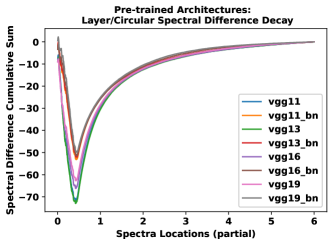
Figure 1: Circular Spectral Difference for vgg architectures. No smoothing, raw histograms. (color online)

III Conjugacy and Equivalence

We introduce a concept of mixed matrix conjugate ensembles inspired from statistical physics Costeniuc et al. (2005); Süzen et al. (2009). Conjugacy of statistical mechanics ensembles are well founded based on Legendre Transforms Costeniuc et al. (2005); Süzen et al. (2009). Here we need to follow a different approach based on core characteristic of a matrix ensembles. There is no known conjugacy rules for such ensembles and we introduce here one of the many possible conjugacy constructions.

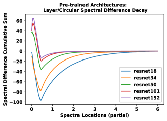
Figure 2: Circular Spectral Difference for resnet architectures. No smoothing, raw histograms. (color online)

Finding an appropriate conjugate mixed matrix ensemble given $\mathscr{L}^{m}$, layer matrix ensemble coming from a trained deep learning architecture or it could be synaptic network weight matrices from Brain networks for example Rajan and Abbott (2006); Bullmore and Sporns (2009) lies in pooled eigenvalues and spectra, see Definition 4. This is a natural way of thinking conjugacy while core properties of matrices usually lies in spectral information of matrix group operators Mudrov (2007).

Definition 4.

The pooled eigenvalues and spectra of mixed matrix ensemble $\mathscr{M}^{m}$ is build from the collection of eigenvalues of $m$ square matrices $A_{i}\in\mathbb{R}^{N_{i}\times N_{i}}$, $i=1,..,m$, denoted by $\epsilon_{j}^{pool}$ and $j=1,...,N_{i}\cdot m$, with a corresponding spectral density $\rho^{pool}(\epsilon)$.

Now, we have well defined setting for defining conjugate ensemble and equivalence condition for MMEs. These are summarized in Definitions 5 and 6.

Definition 5.

Conjugate MMEs
Given two mixed matrix ensembles, $\mathscr{M}_{1}^{m}$ and $\mathscr{M}_{2}^{m}$, forms a conjugate ensembles if their respective cumulative spectral density difference approaches to zero over long positive tail part of the spectrum, Hence at $[0.0,\epsilon_{max}]$, Circular Spectral Difference (CSD), $\Delta_{CSD}(\epsilon)=\rho_{1}(\epsilon)-\rho_{2}(\epsilon)$ and with cumulative CSD defined as $\sum_{0}^{\epsilon_{m}ax}\Delta_{CSD}(\epsilon)$ over spectral locations approaches to zero for large enough $\epsilon_{max}$, The $\epsilon_{max}$ being at least the largest eigenvalue to consider in constructing the spectral density.

Definition 6.

Equivalence of MMEs
Given two mixed matrix ensembles $\mathscr{M}_{1}^{m}$ and $\mathscr{M}_{2}^{m}$ are equivalent if following two conditions met:
1. There is a third mixed matrix ensembles $\mathscr{M}_{c}^{m}$ that is conjugate to both.
2. The variance of Circular Spectral Difference (CSD) of them are equivalent with a small $\delta$,
$Var\left(\Delta_{CSD}^{1}\right)-Var\left(\Delta_{CSD}^{2}\right)=\delta$
. The choice of $\delta$ is an engineering decision that architecture search should decide.

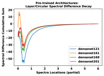
Figure 3: Circular Spectral Difference for densenet architectures. No smoothing, raw histograms. (color online)

IV Experiments with vision architectures

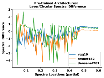
Figure 4: Circular Spectral Difference fluctuations for vgg99, resnet152 and densenet201. (color online)

Our experiments focus on deep neural network architectures developed for vision task. Three different type of vision architectures are used: VGG Simonyan and Zisserman (2014), ResNet He et al. (2016), and DenseNet Huang et al. (2017) with different depth and batch normalisation for VGG. We generated mixed Layer Matrix Ensembles for all mentioned type networks using pretrained weigths Paszke et al. and their corresponding mixed Unitary Circular Ensembles as a proposal conjugate ensembles. We used positive range for long positive tail part of the spectrum $[0,0,6.0]$ with $1000$ equalspacing. This provides sufficiently smooth data with the given pooled eigenvalues from produced ensembles.

Computed CSDs for long positive tail part is shown for VGG, ResNet and DenseNet architectures on Figures 1, 2 and 3 respectively. We observe that different architecture’s CSDs decay in different rates. This indicates different fluctuation characteristics of each CSDs for different architectures as demonstrated on Figure 4.

Variance of all CSDs for all investigated architectures are summarized in Table 1. We clearly see that each architecture type clearly seperated by Variance of CSDs. We see the equivalance of all VGG architectures implying the reported performance metrics are not too far apart in reality, VGG with batch normalisation architectures forms the subset, this is also observed in cumulative CSDs in Figure 1. However the equivalance goes away very quickly with increasing depth, this is observed between resnet18 and resnet152, similarly between densenet121 and densenet201. Equivalence between densenet169 and densenet201 could also be accepted.

V Conclusions

We have developed a methematically well defined approach to detect equivalance between deep learning architectures. The method relies on building conjugate matrix ensembles and investigating their spectral difference over the long positive tail part. This approach can also be used in detecting Brain motifs if synaptic weights are known.

The method is very practical and can be used in designing new artifical neural architectures via Neural Architecture Search (NAS) or compression of the existing known architecture by systematic or random reduction of the network size and computing variance of CSD as proposed in this work. The approach here can be thought as a complexity measure for architecture groups rather than the fine grain complexity measure for a single network, that the group of networks would have similar test performances, hence will be useful in establishing equivalance classes for deep neural networks..

Architecture	Top-1 error	Top-5 error	Variance CSD
vgg11	30.98	11.37	0.19
vgg13	30.07	10.75	0.20
vgg16	28.41	9.63	0.19
vgg19	27.62	9.12	0.18
vgg11bn	29.62	10.19	0.10
vgg13bn	28.45	9.63	0.09
vgg16bn	26.63	8.50	0.10
vgg19bn	25.76	8.15	0.09
resnet18	30.24	10.92	0.20
resnet34	26.70	8.58	0.23
resnet50	23.85	7.13	1.45
resnet101	22.63	6.44	1.86
resnet152	21.69	5.94	1.98
densenet121	25.35	7.83	0.42
densenet161	22.35	6.20	0.29
densenet169	24.00	7.00	0.52
densenet201	22.80	6.43	0.54

Table 1: Variance of CSD per architecture corresponding Top-1 and Top-5 classification errors on ImageNet dataset.

Supplementary material

A Python code notebook with functions to reproduce the data and results is provided with this manuscript, deep_dyson_networks.ipynb.

References

- Rosser (2008) J. B. Rosser, Logic for Mathematicians (Courier Dover Publications, 2008).
- Barré and Gonçalves (2007) J. Barré and B. Gonçalves, Physica A: Statistical Mechanics and its Applications 386, 212 (2007).
- den Hollander et al. (2018) F. den Hollander, M. Mandjes, A. Roccaverde, N. Starreveld, et al., Electronic Journal of Probability 23 (2018).
- Costeniuc et al. (2005) M. Costeniuc, R. S. Ellis, and H. Touchette, Journal of Mathematical physics 46, 063301 (2005).
- Süzen et al. (2009) M. Süzen, M. Sega, and C. Holm, Physical Review E 79, 051118 (2009).
- Chickering (2002) D. M. Chickering, Journal of Machine Learning Research 2, 445 (2002).
- Ertekin and Rudin (2011) Ş. Ertekin and C. Rudin, Journal of Machine Learning Research 12, 2905 (2011).
- Sporns and Kötter (2004) O. Sporns and R. Kötter, PLoS biology 2 (2004).
- Bullmore and Sporns (2009) E. Bullmore and O. Sporns, Nature reviews neuroscience 10, 186 (2009).
- Schmidhuber (2015) J. Schmidhuber, Neural networks 61, 85 (2015).
- LeCun et al. (2015) Y. LeCun, Y. Bengio, and G. Hinton, Nature 521, 436 (2015).
- Elsken et al. (2019) T. Elsken, J. H. Metzen, and F. Hutter, Journal of Machine Learning Research 20, 1 (2019).
- Ren et al. (2020) P. Ren, Y. Xiao, X. Chang, P.-Y. Huang, Z. Li, X. Chen, and X. Wang, arXiv preprint arXiv:2006.02903 (2020).
- Kumar et al. (2019) A. Kumar, T. Serra, and S. Ramalingam, arXiv preprint arXiv:1905.11428 (2019).
- Serra et al. (2020) T. Serra, A. Kumar, and S. Ramalingam, arXiv preprint arXiv:2001.00218 (2020).
- Bubenik (2015) P. Bubenik, The Journal of Machine Learning Research 16, 77 (2015).
- Cang and Wei (2017) Z. Cang and G.-W. Wei, PLoS computational biology 13, e1005690 (2017).
- Rieck et al. (2018) B. Rieck, M. Togninalli, C. Bock, M. Moor, M. Horn, T. Gumbsch, and K. Borgwardt, arXiv preprint arXiv:1812.09764 (2018).
- Wasserman (2018) L. Wasserman, Annual Review of Statistics and Its Application 5, 501 (2018).
- Pennington et al. (2018) J. Pennington, S. S. Schoenholz, and S. Ganguli, arXiv preprint arXiv:1802.09979 (2018).
- Sagun et al. (2017) L. Sagun, U. Evci, V. U. Guney, Y. Dauphin, and L. Bottou, arXiv preprint arXiv:1706.04454 (2017).
- Martin and Mahoney (2019) C. H. Martin and M. W. Mahoney, arXiv preprint arXiv:1901.08276 (2019).
- Süzen et al. (2019) M. Süzen, J. J. Cerdà, and C. Weber, arXiv e-prints , arXiv:1911.07831 (2019), arXiv:1911.07831 [cs.LG] .
- Le Cun et al. (1991) Y. Le Cun, I. Kanter, and S. A. Solla, Physical Review Letters 66, 2396 (1991).
- Mehta (2004) M. L. Mehta, Random Matrices (Elsevier, 2004).
- Wigner (1967) E. P. Wigner, SIAM Review 9, 1 (1967).
- Dyson (1962) F. J. Dyson, Journal of Mathematical Physics 3, 1199 (1962).
- Haake (2013) F. Haake, Quantum Signatures of Chaos, Vol. 54 (Springer Science & Business Media, 2013).
- Süzen et al. (2017) M. Süzen, C. Weber, and J. J. Cerdà, arXiv preprint arXiv:1704.08303 (2017).
- Mezzadri (2006) F. Mezzadri, Notices of AMS 54, 592 (2006).
- Berry and Shukla (2013) M. Berry and P. Shukla, New Journal of Physics 15, 013026 (2013).
- Rajan and Abbott (2006) K. Rajan and L. Abbott, Physical Review Letters 97, 188104 (2006).
- Mudrov (2007) A. Mudrov, Communications in Mathematical Physics 272, 635 (2007).
- Simonyan and Zisserman (2014) K. Simonyan and A. Zisserman, arXiv preprint arXiv:1409.1556 (2014).
- He et al. (2016) K. He, X. Zhang, S. Ren, and J. Sun, in Proceedings of the IEEE conference on computer vision and pattern recognition (2016) pp. 770–778.
- Huang et al. (2017) G. Huang, Z. Liu, L. Van Der Maaten, and K. Q. Weinberger, in Proceedings of the IEEE conference on computer vision and pattern recognition (2017) pp. 4700–4708.
- (37) A. Paszke, S. Gross, F. Massa, A. Lerer, J. Bradbury, G. Chanan, T. Killeen, Z. Lin, N. Gimelshein, L. Antiga, A. Desmaison, A. Kopf, E. Yang, Z. DeVito, M. Raison, A. Tejani, S. Chilamkurthy, B. Steiner, L. Fang, J. Bai, and S. Chintala, in NeurIPS 32, pp. 8024–8035.