Approximation of the Diagonal of a Laplacian’s Pseudoinverse for Complex Network Analysis

Abstract

The ubiquity of massive graph data sets in numerous applications requires fast algorithms for extracting knowledge from these data. We are motivated here by three electrical measures for the analysis of large small-world graphs $G=(V,E)$ – i. e., graphs with diameter in $\mathcal{O}(\log|V|)$, which are abundant in complex network analysis. From a computational point of view, the three measures have in common that their crucial component is the diagonal of the graph Laplacian’s pseudoinverse, $\mathbf{L}^{\dagger}$. Computing $\operatorname{diag}(\mathbf{L}^{\dagger})$ exactly by pseudoinversion, however, is as expensive as dense matrix multiplication – and the standard tools in practice even require cubic time. Moreover, the pseudoinverse requires quadratic space – hardly feasible for large graphs. Resorting to approximation by, e. g., using the Johnson-Lindenstrauss transform, requires the solution of $\mathcal{O}(\log|V|/\epsilon^{2})$ Laplacian linear systems to guarantee a relative error, which is still very expensive for large inputs.

In this paper, we present a novel approximation algorithm that requires the solution of only one Laplacian linear system. The remaining parts are purely combinatorial – mainly sampling uniform spanning trees, which we relate to $\operatorname{diag}(\mathbf{L}^{\dagger})$ via effective resistances. For small-world networks, our algorithm obtains a $\pm\epsilon$-approximation with high probability, in a time that is nearly-linear in $|E|$ and quadratic in $1/\epsilon$. Another positive aspect of our algorithm is its parallel nature due to independent sampling. We thus provide two parallel implementations of our algorithm: one using OpenMP, one MPI + OpenMP. In our experiments against the state of the art, our algorithm (i) yields more accurate approximation results for $\operatorname{diag}(\mathbf{L}^{\dagger})$, (ii) is much faster and more memory-efficient, and (iii) obtains good parallel speedups, in particular in the distributed setting.

1 Introduction

Massive graph data sets are abundant these days in numerous applications. Extracting knowledge from these data thus requires fast algorithms. One common matrix to represent a graph $G=(V,E)$ with $n$ vertices and $m$ edges in algebraic algorithms is its Laplacian $\mathbf{L}=\mathbf{D}-\mathbf{A}$. Here, $\mathbf{D}$ is the diagonal degree matrix with $\mathbf{D}[u,u]$ being the (possibly weighted) degree of vertex $u\in V$. The matrix $\mathbf{A}$ is the (possibly weighted) adjacency matrix of $G$. It is well-known that $\mathbf{L}$ does not have full rank and is thus not invertible. Its Moore-Penrose pseudoinverse [27] $\mathbf{L}^{\dagger}$, in turn, has numerous applications in physics and engineering [62] as well as applied mathematics [27] and graph (resp. matrix) algorithms [40].

We are motivated by one particular class of applications: electrical centrality measures for the analysis of small-world networks – i. e., graphs whose diameter is bounded by $\mathcal{O}(\log n)$. Many important real-world networks (social, epidemiological, information, biological, etc.) have the small-world feature [50]. Centrality measures, in turn, belong to the most widely used network analysis concepts and indicate the importance of a vertex (or edge) in the network [13]. Numerous measures exist, some based on shortest paths, others consider paths of arbitrary lengths. Electrical centrality measures fall into the latter category. They exploit the perspective of graphs as electrical networks (see e. g., [43]). One well-known of such measures is electrical closeness centrality, a. k. a. current-flow closeness or information centrality [17], $c^{el}(\cdot)$. It is the reciprocal of the average effective resistance $\mathbf{r}(u,\cdot)$ between $u$ and all other vertices:

$$c^{el}(u):=\frac{n-1}{\sum_{v\in V\setminus\{u\}}\mathbf{r}(u,v)}.$$ (1)

In an electrical network corresponding to $G$, $\mathbf{r}(u,v)$ is the potential (voltage) difference across terminals $u$ and $v$ when a unit current is applied between them [25]. It can be computed by solving $\mathbf{L}\mathbf{x}=\mathbf{e}_{u}-\mathbf{e}_{v}$ for $\mathbf{x}$, where $\mathbf{e}_{z}$ is the canonical unit vector for vertex $z$. Then, $\mathbf{r}(u,v)=\mathbf{x}[u]-\mathbf{x}[v]$, also see Section 2.1.

Effective resistance also plays a major role in two other electrical measures we consider here, normalized random-walk betweenness [49] and Kirchhoff index centrality [41]. Also note that effective resistance is a graph metric with numerous other applications, well beyond its usage in electrical centralities (cf. Refs. [2, 25]). A straightforward way to compute electrical closeness (or the other two measures) would be to compute $\mathbf{L}^{\dagger}$. Without exploiting structure, this takes $\mathcal{O}(n^{\omega})$ time, where $\omega<2.38$ is the exponent for fast matrix multiplication. The standard tools in practice even require cubic time, cf. [54]. $\mathbf{L}^{\dagger}$ is also in general a dense matrix (also for sparse $\mathbf{L}$). Thus, full (pseudo)inversion is clearly limited to small inputs.

Conceptually similar to inversion would be to solve $\Theta(n)$ Laplacian linear systems. In situations with lower accuracy demands, fewer linear systems suffice: using the Johnson-Lindenstrauss transform (JLT) in connection with a fast Laplacian solver such as Ref. [21], one gets a relative approximation guarantee by solving $\mathcal{O}(\log n/\epsilon^{2})$ systems [59] in $\tilde{\mathcal{O}}(m\log^{1/2}n\log(1/\epsilon))$ time each, where $\tilde{\mathcal{O}}(\cdot)$ hides a $\mathcal{O}((\log\log n)^{3+\delta})$ factor for $\delta>0$.

As pointed out previously [16], the (only) relevant part of $\mathbf{L}^{\dagger}$ for computing electrical closeness is its diagonal (we will see that this is true for other measures as well). Numerical methods for sampling-based approximation of the diagonal of implicitly given matrices do exist [9]. Yet, for our purpose, they solve $\mathcal{O}(\log{n}/\epsilon^{2})$ Laplacian linear systems as well to obtain an $\epsilon$-approximation with high probability, see Section 2.2 for more details.

While this number of Laplacian linear systems can be solved in parallel, their solution can still be time-consuming in practice, in part due to high constants hidden in the $\mathcal{O}$-notation.

Contribution and Outline

We propose a new algorithm for approximating $\operatorname{diag}(\mathbf{L}^{\dagger})$ of a Laplacian matrix $\mathbf{L}$ that corresponds to weighted undirected graphs (Section 3). Our main technique is the approximation of effective resistances between a pivot vertex $u\in V$ and all other vertices of $G$. It is based on sampling uniform (= random) spanning trees (USTs). The resulting algorithm is highly parallel and (almost) purely combinatorial – it relies on the connection between Laplacian linear systems, effective resistances, and USTs.

For small-world graphs, our algorithm obtains an absolute $\pm\epsilon$-approximation guarantee with high probability in (sequential) time $\mathcal{O}(m\log^{4}n\cdot\epsilon^{-2})$. In particular, compared to using the fastest theoretical Laplacian solvers in connection with JLT, our approach is off by only a polylogarithmic factor. Probably more importantly, after some algorithm engineering (Section 4), our algorithm performs much better than the state of the art, already in our sequential experiments (Section 5): (i) it is much faster and more memory-efficient, (ii) it yields a maximum absolute error that is one order of magnitude lower, and (iii) results in a more accurate complete centrality ranking of elements of $\operatorname{diag}(\mathbf{L}^{\dagger})$. Due to good parallel speedups, we can even compute a reasonably accurate diagonal of $\mathbf{L}^{\dagger}$ on a small-scale cluster with 16 compute nodes in less than 8 minutes for a graph with $\approx 13.6$M vertices and $\approx 334.6$M edges. Material omitted from the main part can be found in the appendix.

2 Preliminaries

2.1 Problem Description and Notation

We type vectors and matrices in bold font. As input we consider simple, finite, connected undirected graphs $G=(V,E)$ with $n$ vertices, $m$ edges, and non-negative edge weights $\mathbf{w}\in\mathbb{R}_{\geq 0}^{m}$. For the complexity analysis, we usually assume that the diameter of $G$ is $\mathcal{O}(\log n)$, but our algorithm would also work correctly without this assumption.

Graphs as electrical networks

We interpret $G$ as an electrical network in which every edge $e\in E$ represents a resistor with resistance $1/\mathbf{w}[e]$. In this context, it is customary to fix an arbitrary orientation $E^{\pm}$ of the edges in $E$ and to define a unit $s$-$t$-current flow (also called electrical flow) in this network as a function of the edges (written as vector) $\mathbf{f}\in\mathbb{R}_{\geq 0}^{|E^{\pm}|}$. Whenever possible, we use $\mathbf{f}[u,v]$ as shorthand notation for $\mathbf{f}[\{u,v\}]$ or $\mathbf{f}[(u,v)]$. Note that $\mathbf{f}[e]=-\mathbf{f}[-e]$ for $e\notin E^{\pm}$. This sign change in the $s$-$t$ current when the flow direction is changed, is required to adhere to Kirchhoff’s current law on flow conservation:

$$\sum_{w\in\delta^{+}(v)}\mathbf{f}[v,w]-\sum_{u\in\delta^{-}(v)}\mathbf{f}[u,v]=\begin{cases}1&\text{if }v=s\\ -1&\text{if }v=t\\ 0&\text{otherwise,}\end{cases}$$ (2)

where $\delta^{+}(v)$ [$\delta^{-}(v)$] is the set of edges having $v$ as head [tail] in the orientation we choose in $E^{\pm}$. Such a flow also adheres to Kirchhoff’s voltage law (sum in cycle is zero when considering flow directions) and Ohm’s law (potential difference = resistance $\cdot$ current), cf. [45, 14]. The effective resistance between two vertices $u$ and $v$, $\mathbf{r}(u,v)$, is defined as the potential difference between $u$ and $v$ when a unit current is injected into $G$ at $u$ and extracted at $v$, comp. [14, Ch. IX]. To compute $\mathbf{r}(u,v)$, let $\mathbf{e}_{z}$ be the canonical unit vector for vertex $z$, i. e., $\mathbf{e}_{z}(z)=1$ and $\mathbf{e}_{v}=0$ for all vertices $v\neq z$. Then,

$$\mathbf{r}(u,v)=(\mathbf{e}_{u}-\mathbf{e}_{v})^{T}\mathbf{L}^{\dagger}(\mathbf{e}_{u}-\mathbf{e}_{v})=\mathbf{\mathbf{L}^{\dagger}}[u,u]-2\mathbf{\mathbf{L}^{\dagger}}[u,v]+\mathbf{\mathbf{L}^{\dagger}}[v,v]$$ (3)

or, equivalently, $\mathbf{r}(u,v)=\mathbf{x}[u]-\mathbf{x}[v]$, where $\mathbf{x}$ is the solution vector of the Laplacian linear system $\mathbf{L}\mathbf{x}=\mathbf{e}_{u}-\mathbf{e}_{v}$. The Laplacian pseudoinverse, $\mathbf{L}^{\dagger}$, can be expressed as $\mathbf{L}^{\dagger}=(\mathbf{L}+\frac{1}{n}\mathbf{J})^{-1}-\frac{1}{n}\mathbf{J}$ [62], where $\mathbf{J}$ is the $n\times n$-matrix with all entries being $1$.

Also note that the effective resistance between the endpoints of an edge $e\in E$ equals the probability that $e$ is an edge in a uniform spanning tree (UST), i. e., a spanning tree selected uniformly at random among all spanning trees of $G$, cf. [14, Ch. II].

Electrical Closeness

The combinatorial counterpart of electrical closeness is based on shortest-path distances $\operatorname{dist}(u,v)$ for vertices $u$ and $v$ in $G$: $c^{c}(u):=\left(n-1\right)/f^{c}(u)$, where the denominator is the combinatorial farness of $u$:

$$f^{c}(u):=\sum_{v\in V\setminus\{u\}}\operatorname{dist}(u,v).$$ (4)

Electrical farness $f^{el}(\cdot)$ is defined analogously to combinatorial farness – shortest-path distances in Eq. (4) are replaced by effective resistances $\mathbf{r}(u,v)$. Closeness centrality (both combinatorial and electrical) are not defined for disconnected graphs due to infinite distances. We can get around this, however: a combinatorial generalization for closeness called Lin’s index (cf. [10]) can be adapted to the electrical case, too. Thus, our assumption of $G$ being connected is no limitation.

Normalized Random-Walk Betweenness

Classical betweenness, based on shortest paths, is one of the most popular centrality measures. The betweenness of vertices using random-walk routing instead of shortest paths is given by the normalized random-walk betweenness (NRWB) [49]. This measure counts each random walk passing through a vertex only once. By mapping the random walk problem to current flowing in a network, Ref. [49] obtains a closed-form expression of NRWB and provides an analysis of its scaling behavior as a function of $n$. Then, the NRWB $c_{b}(\cdot)$ of a vertex $v$ is:

$$c_{b}(v)=\frac{1}{n}+\frac{1}{n-1}\sum_{t\neq v}\frac{\mathbf{M^{-1}}[t,t]-\mathbf{M^{-1}}[t,v]}{\mathbf{M^{-1}}[t,t]+\mathbf{M^{-1}}[v,v]-2\mathbf{M^{-1}}[t,v]},$$ (5)

where $\mathbf{M}:=\mathbf{L}+\mathbf{P}$, with $\mathbf{P}$ the projection operator onto the zero eigenvector of the Laplacian $\mathbf{L}$ such that $\mathbf{P}[i,j]=1/n$. We show in Section 3.4 how to simplify this expression.

We also consider the Kirchhoff index and related centrality measures. Their description can be found in Appendix B.1.

2.2 Related Work

Solving Laplacian Systems

A straightforward approach to compute electrical closeness and related centralities is to compute $\mathbf{L}^{\dagger}$, by solving a number of Laplacian systems. Brandes and Fleischer [17] computed electrical closeness from the solution of $n$ linear systems using conjugate gradient (CG) in $\mathcal{O}(mn\sqrt{\kappa})$ time, where $\kappa$ is the condition number of the appropriately preconditioned Laplacian matrix. Later, Spielman and Srivastava proposed an approximation algorithm for computing effective resistance distances [59]. The main ingredients of the algorithm are a dimension reduction with Johnson-Lindenstrauss [31] and the use of a fast Laplacian solver for $\mathcal{O}(\log{n}/\epsilon^{2})$ Laplacian systems. The algorithm approximates effective resistance values for all edges within a factor of $(1\pm\epsilon)$ in $\mathcal{O}(I(n,m)\log{n}/\epsilon^{2})$ time, where $I(n,m)$ is the running time of the Laplacian solver, assuming that the solution of the Laplacian systems is exact. With an approximate Laplacian solution, the algorithm yields a $(1+\epsilon)^{2}$-approximation. Significant progress in the development of fast Laplacian solvers with theoretical guarantees [34, 35, 32, 21, 39] has resulted in the currently best one running in $\mathcal{O}(m\log^{1/2}{n}\log(1/\epsilon))$ time (up to polylogarithmic factors) [21]. Parallel algorithms for solving linear systems on the more general SDD matrices also exist in the literature [53, 12]. To date, the fastest algorithms for electrical closeness and spanning edge centrality extend the idea of Spielman and Srivastava [11, 47, 29]. (Similar ideas are used for centrality measures based on the Kirchhoff index, see Appendix B.2). Since theoretical Laplacian solvers rely on heavy graph-theoretic machinery such as low-stretch spanning trees, one rather uses multigrid solvers [42, 11, 36] in practice instead.

Diagonal Estimation

Recall from the introduction that the diagonal (or in case of the Kirchhoff index even only its sum, the trace – see Appendix B.1) of $\mathbf{L}^{\dagger}$ is enough to compute electrical closeness and related measures, also see Eq. (6) below. Algorithms that approximate the diagonal (or the trace) of matrices that are only implicitly available often use iterative methods [58], sparse direct methods [3, 30], Monte Carlo [24] or deterministic probing techniques [61, 9]. A popular approach is the standard Monte-Carlo method for the trace of $\mathbf{A}$, due to Hutchinson [24]. The idea is to estimate the trace of $\mathbf{A}$ by observing the action of $\mathbf{A}$ (in terms of matrix-vector products) on a sufficiently large sample of random vectors $r_{k}$. In our case, this would require to solve a large number of Laplacian linear systems with vectors $r_{k}$ as right-hand sides. Avron and Toledo [6] proved that the method takes $\mathcal{O}(\log{n}/\epsilon^{2})$ samples to achieve a maximum error $\epsilon$ with probability at least $1-\delta$. The approach from Hutchinson [24] has been extended by Bekas et al. [9] for estimating the diagonal of $\mathbf{A}$. Finally, Barthelmé et al. [8] have recently proposed a combinatorial algorithm to approximate the trace (not the diagonal) of the inverse of a matrix closely related to the Laplacian. Their algorithm can be seen as a special case of our algorithm in the situation where a universal vertex exists.

Normalized Random Walk Betweenness

Along with the introduction of the measure, Ref. [49] provided numerical evaluations of Eq. (5) on various graph models. However, no algorithm to compute the measure without (pseudo)inverting $\mathbf{L}$ has been proposed yet.

3 Approximation Algorithm

3.1 Overview

In order to compute the electrical closeness for all vertices in $V(G)$, the main challenge is obviously to compute their electrical farness, $f^{el}(\cdot)$. Recall from the introduction that the diagonal of $\mathbf{L}^{\dagger}$ is sufficient to compute $f^{el}(\cdot)$ for all vertices simultaneously (comp. Ref. [16, Eq. (15)] with a slightly different definition of electrical closeness). This follows from Eq. (3) and the fact that each row/column in $\mathbf{L}^{\dagger}$ sums to $0$:

$$\begin{split}f^{el}(u)&:=\sum_{v\in V\setminus\{u\}}\mathbf{r}(u,v)=n\cdot\mathbf{\mathbf{L}^{\dagger}}[u,u]+\operatorname{tr}(\mathbf{L}^{\dagger})-2\sum_{v\in V}\mathbf{\mathbf{L}^{\dagger}}[u,v]=n\cdot\mathbf{\mathbf{L}^{\dagger}}[u,u]+\operatorname{tr}(\mathbf{L}^{\dagger}),\end{split}$$ (6)

since the trace $\operatorname{tr}(\cdot)$ is the sum over the diagonal entries.

We are interested in an approximation of $\operatorname{diag}(\mathbf{L}^{\dagger})$, since we do not necessarily need exact values for our particular applications. To this end, we propose an approximation algorithm for which we give a rough overview first. Our algorithm works best for small-world networks – thus, we focus on this important input class. Let $G$ be unweighted for now; we discuss the extension to weighted graphs in Section 3.4.

1. Select a pivot vertex $u\in V$ and solve the linear system $\mathbf{L}\mathbf{x}=\mathbf{e}_{u}-\frac{1}{n}\cdot\mathbf{1}$, where $\mathbf{1}=(1,\dots,1)^{T}$. Out of all solutions $\mathbf{x}$, we want the one such that $\mathbf{x}\perp\mathbf{1}$, since this unique normalized solution is equal to $\mathbf{\mathbf{L}^{\dagger}}[:,u]$, the column of $\mathbf{L}^{\dagger}$ corresponding to $u$, also see Ref. [62, pp. 6-7].

2. Throughout the rest of this paper we denote $V^{\prime}:=V\setminus\{u\}$. As a direct consequence from Eq. (3), the diagonal entries $\mathbf{\mathbf{L}^{\dagger}}[v,v]$ for all $v\in V^{\prime}$ can be computed as:

   $$\mathbf{\mathbf{L}^{\dagger}}[v,v]=\mathbf{r}(u,v)-\mathbf{\mathbf{L}^{\dagger}}[u,u]+2\mathbf{\mathbf{L}^{\dagger}}[v,u].$$ (7)

3. It remains to approximate these $n-1$ effective resistance values $\mathbf{r}(\cdot,\cdot)$. In order to do so, we employ Kirchhoff’s theorem, which connects electrical flows with spanning trees [14, Ch. II]. To this end, let $N$ be the total number of spanning trees of $G$; moreover, let $N_{s,t}(a,b)$ be the number of spanning trees in which the unique path from $s$ to $t$ traverses the edge $\{a,b\}$ in the direction from $a$ to $b$.

   Theorem 3.1 (Kirchhoff, comp. [14]).

   Let $\mathbf{f}[a,b]:=(N_{s,t}(a,b)-N_{s,t}(b,a))/N$. Distribute current flows on the edges of $G$ by sending a current of size $\mathbf{f}[a,b]$ from $a$ to $b$ for every edge $\{a,b\}$. Then there is a total current of size $1$ from $s$ to $t$ satisfying Kirchhoff’s laws.

   As a result of Theorem 3.1, the effective resistance between $s$ and $t$ is the potential difference between $s$ and $t$ induced by the current-flow given by $\mathbf{f}$. Vice versa, since the current flow is induced by potential differences (Ohm’s law), one simply has to add the currents on a path from $s$ to $t$ to compute $\mathbf{r}(s,t)$ (see Eq. (8) in Section 3.2). Actually, as a proxy for the current flows, we use the (approximate) $N(\cdot)$-values mentioned in Theorem 3.1.

4. It is impractical to compute exact values for $N$ (e. g., by Kirchhoff’s matrix-tree theorem [26], which would require the determinant or all eigenvalues of $\mathbf{L}^{\dagger}$) or $N(\cdot)$ for large graphs. Instead, we obtain approximations of the desired values via sampling: we sample a set of uniform spanning trees and determine the $N(\cdot)$-values by aggregation over all sampled trees. This approach provides a probabilistic absolute approximation guarantee.

The pseudocode of the algorithm, in adjusted order, is shown and discussed as Algorithm 1 in Appendix A.1. Components and properties of Algorithm 1 are explained in the remainder of Section 3; reading Section 3.2 while/before studying the pseudocode is recommended.

Note that Steps 2-4 of the algorithm are entirely combinatorial. Step 1 may or may not be combinatorial, depending on the Laplacian solver used. Corresponding implementation choices are discussed in Section 4.

3.2 Effective Resistance Approximation by UST Sampling

Extending and generalizing work by Hayashi et al. [29] on spanning edge centrality, our main idea is to compute a sufficiently large sample of USTs and to aggregate the $N(\cdot)$-values of the edges in these USTs. Given $G$ and an electrical flow with source $u$ and sink $v$, recall that the effective resistance between them is the potential difference $\mathbf{x}[u]-\mathbf{x}[v]$, where $\mathbf{x}$ is the solution vector in $\mathbf{L}\mathbf{x}=\mathbf{e}_{u}-\mathbf{e}_{v}$. Since $\mathbf{x}$ is a potential and the electrical flow $\mathbf{f}$ results from its difference, $\mathbf{r}(u,v)$ can be computed given any path $\langle u=v_{0},v_{1},\dots,v_{k-1},v_{k}=v\rangle$ as:

$$\begin{split}\mathbf{r}(u,v)&=\sum_{i=0}^{k-1}\mathbf{f}[v_{i},v_{i+1}]\\ &=1/N\sum_{i=0}^{k-1}\left(N_{u,v}(v_{i},v_{i+1})-N_{u,v}(v_{i+1},v_{i})\right).\end{split}$$ (8)

Recall that the sign of the current flow changes if we traverse an edge against the flow direction. This is reflected by the second summand in the sum of Eq. (8). Since we can choose any path from $u$ to $v$, for efficiency reasons we use one shortest path $P(v)$ per vertex $v\in V^{\prime}$. We compute these paths with one breadth-first search (BFS) with root $u$, resulting in a tree $B_{u}$ whose edges are considered as implicitly directed from the root to the leaves. For each vertex $v\in V^{\prime}$, we maintain an estimate $R[v]$ of $\mathbf{r}(u,v)$, which is initially set to $0$ for all $v$. After all USTs have been processed, we divide all entries of $R$ by $\tau$, the number of sampled trees, i. e., $\tau$ takes the role of $N$ in Eq. (8).

Sampling USTs

In total, we sample $\tau$ USTs, where $\tau$ depends on the desired approximation guarantee and is determined later. The choice of the UST algorithm depends on the input: for general graphs, the algorithm by Schild [55] with time complexity $\mathcal{O}(m^{1+o(1)})$ is the fastest. Among others, it uses a sophisticated shortcutting technique using fast Laplacian solvers to speed up the classical Aldous-Broder [1, 18] algorithm. For unweighted small-world graphs, however, Wilson’s simple algorithm using loop-erased random walks is in $\mathcal{O}(m\log n)$, as outlined in Appendix A.2. Thus, for our class of inputs, Wilson’s algorithm is preferred.

Data structures

When computing the contribution of a UST $T$ to $N(\cdot)$, we need to update for each edge $e=(a,b)\in E(T)$ its contribution to $N_{u,v}(a,b)$ and $N_{u,v}(b,a)$, respectively – for exactly every vertex $v$ for which $(a,b)$ [or $(b,a)$] lies on $P(v)$. Hence, the algorithm that aggregates the contribution of UST $T$ to $R$ will need to traverse $P(v)$ for each vertex $v\in V$. To this end, we represent the BFS tree $B_{u}$ as an array of parent pointers for each vertex $v\in V$. On the other hand, the tree $T$ can conveniently be represented by storing a child and a sibling for each vertex $v\in V$. Compared to other representations (such as adjacency lists), this data structure can be constructed and traversed with low constant overhead.

Tree Aggregation

After constructing a UST $T$, we process it to update the intermediate effective resistance values $R[\cdot]$. Note that we can discard $T$ afterwards and do not have to store the full sample, which has a positive effect on the memory footprint of our algorithm. The aggregation algorithm is shown as Algorithm 2 in Appendix A.1. Recall that we need to determine for each vertex $v$ and each edge $(a,b)\in P(v)$, whether $(a,b)$ or $(b,a)$ occurs on the unique $u$-$v$ path in $T$. To simplify this test, we root $T$ at $u$; hence, it is enough to check if $(a,b)$ [or $(b,a)$] appears above $v$ in $T$. For general graphs, the test still incurs quadratic overhead in running time (in particular, the number of vertex-edge pairs that need to be considered is $f^{c}(u)=\sum_{v\in V^{\prime}}|P(v)|=\mathcal{O}(n^{2})$). We remark that, perhaps surprisingly, a bottom-up traversal of $T$ does not improve on this, either; it is similarly difficult to determine all $R[v]$ that a given $(a,b)\in E(T)$ contributes to (those $v$ form an arbitrary subset of descendants of $b$ in $T$). However, we can exploit the fact that on small-world networks, the depth of $B_{u}$ can be controlled, i. e., $f^{c}(u)$ is sub-quadratic. To accelerate the test, we first compute a DFS data structure for $T$, i. e., we determine discovery and finish timestamps for all vertices in $V$, respectively. For an arbitrary $v\in V$ and $(a,b)\in V\times V$, this data structure allows us to answer in constant time (i) whether either $(a,b)$ or $(b,a)$ is in $T$ and (ii) if $(a,b)\in E(T)$, whether $v$ appears below $(a,b)$ in $T$. Finally, we loop over all $v\in V$ and all $e=(a,b)\in P(v)$ and aggregate the contribution of $T$ to $N_{u,v}(a,b)$. To do so, we add [subtract] $1$ to [from] $R[v]$ if $e$ has the same [opposite] direction in $B_{u}$. If $e$ is not in $B_{u}$, $R[v]$ does not change.

3.3 Algorithm Analysis

The choice of the pivot $u$ has an effect on the time complexity of our algorithm. The intuitive reason is that the BFS tree $B_{u}$ should be shallow in order to have short paths to the root $u$, which is achieved by a $u$ with small eccentricity. The proofs of this subsection can be found in Appendices A.3 and A.4. Regarding aggregation, we obtain:

Lemma 3.2.

Tree aggregation (Algorithm 2 in Appendix A.1) has time complexity $\mathcal{O}(f^{c}(u))$, which can be bounded by $\mathcal{O}(n\cdot\operatorname{ecc}(u))=\mathcal{O}(n\cdot\operatorname{diam}(G))$.

In high-diameter networks, the farness of $u$ can become quadratic (consider a path graph) and thus problematic for large inputs. In small-world graphs, however, we obtain $\mathcal{O}(n\log n)$ per aggregation. We continue the analysis with the main algorithmic result.

Theorem 3.3.

Let $G$ be an undirected and unweighted graph with $n$ vertices, $m$ edges, diameter $\operatorname{diam}(G)$ and Laplacian $\mathbf{L}=\mathbf{L}(G)$. Then, our diagonal approximation algorithm (Algorithm 1 in Appendix A.1) computes an approximation of $\operatorname{diag}(\mathbf{L}^{\dagger})$ with absolute error $\pm\epsilon$ with probability $1-\delta$ in time $\mathcal{O}(m\cdot\operatorname{ecc}^{3}(u)\cdot\epsilon^{-2}\cdot\log(m/\delta))$. For small-world graphs and with $\delta:=1/n$ to get high probability, this yields a time complexity of $\mathcal{O}(m\log^{4}n\cdot\epsilon^{-2}$).

Thus, for small-world networks, we have an approximation algorithm whose running time is nearly-linear in $m$ (i. e., linear up to a polylogarithmic factor), quadratic in $1/\epsilon$, and logarithmic in $1/\delta$. By choosing a ?good? pivot $u$, it is often possible to improve the running time of Algorithm 1 by a constant factor (i. e., without affecting the $\mathcal{O}$-notation). In particular, there are vertices $u$ with $\operatorname{ecc}(u)$ as low as $\frac{1}{2}\operatorname{diam}(G)$. A discussion on the algorithm’s parallelization in the work-depth model can be found in Appendix A.1.2.

Remark 3.4.

If $G$ has constant diameter, Algorithm 1 has time complexity $\mathcal{O}(m\log n\cdot\epsilon^{-2})$ to obtain an absolute $\epsilon$-approximation guarantee. This is faster than the best JLT-based approximation (which provides a relative guarantee instead).

3.4 Generalizations

In this section we show how our algorithm can be adapted to work for weighted graphs and for normalized random-walk betweenness as well. The extensions to Kirchhoff-related indices are presented in Appendix B.3.

Extension to Weighted graphs

For an extension to weighted graphs, we need a weighted version of Kirchhoff’s theorem. To this end, the weight of a spanning tree $T$ is defined as the product of the weights (= conductances) of its edges. Then, let $N^{*}$ be the sum of the weights of all spanning trees of $G$; also, let $N^{*}_{s,t}(a,b)$ be the sum of the weights of all spanning trees in which the unique path from $s$ to $t$ traverses the edge $\{a,b\}$ in the direction from $a$ to $b$.

Theorem 3.5 (comp. [14], p. 46).

There is a distribution of currents satisfying Ohm’s law and Kirchhoff’s laws in which a current of size $1$ enters at $s$ and leaves at $t$. The value of the current on edge $\{a,b\}$ is given by $(N^{*}_{s,t}(a,b)-N^{*}_{s,t}(b,a))/N^{*}$.

Consequently, our sampling approach needs to estimate $N^{*}$ as well as the $N^{*}(\cdot)$-values. It turns out that no major changes are necessary. Wilson’s algorithm also yields a UST for weighted graphs (if its random walk takes edge weights for transition probabilities into account) [64]. Yet, the running time bound for Wilson needs to mention the graph volume, $\operatorname{vol}(G)$, explicitly now: $\mathcal{O}(\operatorname{ecc}(u)\cdot\operatorname{vol}(G))$. The weight of each sampled spanning tree can be accumulated during each run of Wilson. It has to be integrated into Algorithm 2 by adding [subtracting] the tree weight in Line 9 [Line 12] instead of 1. For the division at the end, one has to replace $\tau$ by the total weight of the sampled trees. Finally, the tree $B_{u}$ remains a BFS tree. The eccentricity and farness of $u$ then still refer in the analysis to their unweighted versions, respectively, as far as $B_{u}$ is concerned.

To conclude, the only important change regarding bounds happens in Theorem 3.3. In the time complexity, $m$ is replaced by $\operatorname{vol}(G)$.

Normalized Random-Walk Betweenness

Ref. [49] proposes normalized random-walk betweenness as a measure for the influence of a vertex in the network, but the paper does not provide an algorithm (beyond implicit (pseudo)inversion). We propose to compute normalized random-walk betweenness with Algorithm 1 and derive (proof in Appendix A.5):

Lemma 3.6.

Normalized random-walk betweenness $c_{b}(v)$ (Eq. (5)) can be rewritten as:

$$c_{b}(v) =\frac{1}{n}+\frac{\operatorname{tr}(\mathbf{L}^{\dagger})}{(n-1)f^{el}(v)}.$$ (9)

Hence, since Algorithm 1 approximates the diagonal of $\mathbf{L}^{\dagger}$ and both trace and electrical farness depend only on the diagonal, the following proposition holds:

Proposition 3.7.

Let $G=(V,E)$ be a small-world graph as in Theorem 3.3. Then, Algorithm 1 approximates with high probability $c_{b}(v)$ for all $v\in V$ with absolute error $\pm\epsilon$ in $\mathcal{O}(m\log^{4}n\cdot\epsilon^{-2})$ time.

4 Engineering Aspects and Parallelization

Important engineering decisions concern the choice of the UST sampling algorithm, decomposition of the input graph into biconnected components, selection of the pivot $u$, and the linear solver used for the initial linear system. For these aspects, we refer the reader to Appendix C.1.

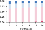
Figure 5: Breakdown of the running times of UST with $\epsilon=0.3$ w. r. t. #of cores on $1\times 24$ cores. Data is aggregated with the geometric mean over the instances of Tables 2 and 3 (see full version [4]).

Our implementation uses OpenMP for shared memory and MPI+OpenMP for distributed memory. We assume that the entire graph fits into main memory (even in the distributed case). Hence, we can parallelize Algorithm 1 to a large extent by sampling and aggregating multiple USTs in parallel. In particular, we turn the main sampling loop into a parallel for loop. We also solve the initial Laplacian system using a shared-memory parallel Conjugate Gradient (CG) solver (see Appendix C.1). Note that we do not employ parallelism in the other steps of the algorithm. In particular, the BFS to compute $B_{u}$ is executed sequentially. We also do not parallelize over the loops in Algorithm 2 to avoid nested parallelism with multiple invocations of Algorithm 2. We note that, in contrast to the theoretical work-depth model, solving the initial Laplacian system and performing the BFS are not the main bottlenecks in practice. Instead, sampling and aggregating USTs together consume the majority of CPU time (see Figure 5 in Appendix E.1. More details regarding shared and distributed memory, in particular load balancing for the distributed case, are discussed in Appendix C.2.

5 Experiments

5.1 Settings

We conduct experiments to demonstrate the performance of our approach compared to the state-of-the-art competitors. Unless stated otherwise, we implemented all algorithms in C++, using the NetworKit [60] graph APIs. Our own algorithm is labelled UST in the sections below. All experiments were conducted on a cluster with 16 Linux machines, each equipped with an Intel Xeon X7460 CPU (2 sockets, 12 cores each), and 192 GB of RAM. To ensure reproducibility, all experiments were managed by the SimexPal [5] software. We executed our experiments on the graphs in Tables 2, 3, 4, and 5 in Appendix D.2. All of them are unweighted and undirected. They have been downloaded from the public KONECT [37] repository and reduced to their largest connected component.

Quality Measures and Baseline

To evaluate the diagonal approximation quality, we measure the maximum absolute error ($\max_{i}\mathbf{L}^{\dagger}_{ii}-\widetilde{\mathbf{L}^{\dagger}_{ii}}$) on each instance, and we take both the maximum and the arithmetic mean over all the instances. Since for some applications [50, 51] a correct ranking of the entries is more relevant than their scores, in our experimental analysis we compare complete rankings of the elements of $\widetilde{\mathbf{L}^{\dagger}}$. Note that the lowest entries of $\mathbf{L}^{\dagger}$ (corresponding to the vertices with highest electrical closeness) are distributed on a significantly narrow interval. Hence, to achieve an accurate electrical closeness ranking of the top $k$ vertices, one would need to solve the problem with very high accuracy. For this reason, all approximation algorithms we consider do not yield a precise top-$k$ ranking, so that we (mostly) consider the complete ranking.

Using pinv in NumPy or Matlab as a baseline would be too expensive in terms of time (cubic) and space (quadratic) on large graphs (see Appendix D.2). Thus, as quality baseline we employ the LAMG solver [42] (see also next paragraph) as implemented within NetworKit [11] in our experiments (with $10^{-9}$ tolerance). The results in Table 6 in Appendix E.4 indicate that the diagonal obtained this way is sufficiently accurate.

Competitors in Practice

In practice, the fastest way to compute electrical closeness so far is to combine a dimension reduction via the Johnson-Lindenstrauss lemma [31] (JLT) with a numerical solver. In this context, Algebraic MultiGrid (AMG) solvers exhibit better empirical running time than fast Laplacian solvers with a worst-case guarantee [47]. For our experiments we use JLT combined with LAMG [42] (named Lamg-jlt); the latter is an AMG-type solver for complex networks. We also compare against a Julia implementation of JLT together with the fast Laplacian solver proposed by Kyng et al. [38], for which a Julia implementation is already available in the package Laplacians.jl. This solver generates a sparse approximate Cholesky decomposition for Laplacian matrices with provable approximation guarantees in $\mathcal{O}(m\log^{3}{n}\log(1/\epsilon))$ time; it is based purely on random sampling (and does not make use of graph-theoretic concepts such as low-stretch spanning trees or sparsifiers). We refer to the above implementation as Julia-jlt throughout the experiments. For both Lamg-jlt and Julia-jlt, we try different input error bounds (they correspond to the respective numbers next to the method names in Figure 1). This is a relative error, since these algorithms use numerical approaches with a relative error guarantee, instead of an absolute one (see Appendix E for results in terms of different quality measures).

Finally, we compare against the diagonal estimators due to Bekas et al. [9], one based on random vectors and one based on Hadamard rows. To solve the resulting Laplacian systems, we use LAMG in both cases. In our experiments, the algorithms are referred to as Bekas and Bekas-h, respectively. Excluded competitors are discussed in Appendix D.1.

5.2 Running Time and Quality

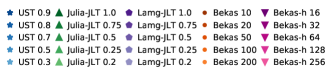
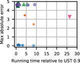
(a) Maximum of the maximum absolute errors.

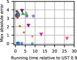
(b) Arithmetic mean of the maximum absolute error.

(c) Geometric mean of the percentage of inverted pairs in the full ranking of $\operatorname{diag}(\mathbf{L}^{\dagger})$.

Figure 1: Quality results over the instances of Table 2. All runs are sequential.

Figure 1(a) shows that, in terms of maximum absolute error, every configuration of UST achieves results with higher quality than the competitors. Even when setting $\epsilon=0.9$, UST yields a maximum absolute error of $\numprint{0.09}$, and it is $\numprint{8.3}\times$ faster than Bekas with 200 random vectors, which instead achieves a maximum absolute error of $\numprint{2.43}$. Furthermore, the running time of UST does not increase substantially for lower values of $\epsilon$, and its quality does not deteriorate quickly for higher values of $\epsilon$. Regarding the average of the maximum absolute error, Figure 1(b) shows that, among the competitors, Bekas-h with 256 Hadamard rows achieves the best precision. However, UST yields an average error of $\numprint{0.07}$ while also being $\numprint{25.4}\times$ faster than Bekas-h, which yields an average error of $\numprint{0.62}$. Note also that the number next to each method in Figure 1 corresponds to different values of absolute (for UST) or relative (for Lamg-jlt, Julia-jlt) error bounds, and different numbers of samples (for Bekas, Bekas-h). For Bekas-h the number of samples needs to be a multiple of four due to the dimension of Hadamard matrices.

In Figure 1(c) we report the percentage of inverted pairs in the full ranking of $\widetilde{\mathbf{L}^{\dagger}}$. Note that JLT-based approaches are not depicted in this plot, because they yield $>15\%$ of rank inversions. Among the competitors, Bekas achieves the best time-accuracy trade-off. However, when using 200 random vectors, it yields $\numprint{4.3}\%$ inversions while also being $\numprint{8.3}\times$ slower than UST with $\epsilon=0.9$, which yields $\numprint{2.1}\%$ inversions only.

For validation purposes, we also measure how well the considered algorithms compute the set (not the ranking) of top-$k$ vertices, i. e., those with highest electrical closeness centrality, with $k\in\{10,100\}$. For each algorithm we only consider the parameter settings that yields the highest accuracy. JLT-based approaches appear to be very accurate for this purpose, as their top-$k$ sets achieve a Jaccard index of $1.0$. As expected (due to its absolute error guarantee), UST performs slightly worse: on average, it obtains 0,95 for $k=10$ and 0,98 for $k=100$, which still shows a high overlap with the ground truth.

The memory consumption is shown and discussed in more detail in Appendix E.3. In summary, as our algorithm can discard each UST after its aggregation, it is rather space-efficient and requires less memory than the competitors.

5.3 Parallel Scalability

The log-log plot in Figure 4(a) (Appendix E.1) shows that on shared-memory UST achieves a moderate parallel scalability w. r. t. the number of cores; on 24 cores in particular it is $\numprint{11.9}\times$ faster than on a single core. Even though the number of USTs to be sampled can be evenly divided among the available cores, we do not see a nearly-linear scalability: on multiple cores the memory performance of our NUMA system becomes a bottleneck. Therefore, the time to sample a UST increases and using more cores yields diminishing returns. Limited memory bandwidth is a known issue affecting algorithms based on graph traversals in general [7, 44]. Finally, we compare the parallel performance of UST indirectly with the parallel performance of our competitors. More precisely, assuming a perfect parallel scalability for our competitors Bekas and Bekas-h on 24 cores, UST would yield results 4,1 and 12,6 times faster, respectively, even with this strong assumption for the competition’s benefit.

UST scales better in a distributed setting. In this case, the scalability is affected mainly by its non-parallel parts and by synchronization latencies. The log-log plot in Figure 4(b) shows that on up to 4 compute nodes the scalability is almost linear, while on 16 compute nodes UST achieves a $\numprint{15.1}\times$ speedup w. r. t. a single compute node.

Figure 5 in Appendix E.1 shows the fraction of time that UST spends on different tasks depending on the number of cores. We aggregated over “Sequential Init.” the time spent on memory allocation, pivot selection, solving the linear system, the computation of the biconnected components, and on computing the tree $B_{u}$. In all configurations, UST spends the majority of the time in sampling, computing the DFS data structures and aggregating USTs. The total time spent on aggregation corresponds to “UST aggregation” and “DFS” in Figure 5, indicating that computing the DFS data structures is the most expensive part of the aggregation. Together, sampling time and total aggregation time account for $\numprint{99.4}\%$ and $\numprint{95.3}\%$ of the total running time on 1 core and 24 cores, respectively. On average, sampling takes $\numprint{66.8}\%$ of this time, while total aggregation takes $\numprint{31.2}\%$. Since sampling a UST is on average $\numprint{2.2}\times$ more expensive than computing the DFS timestamps and aggregation, faster sampling techniques would significantly improve the performance of our algorithm.

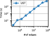
(a) Running time of UST w. r. t. #of edges.

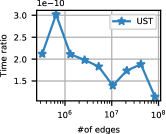
(b) Ratio of running time of UST w. r. t. its theoretical running time (see Theorem 3.3).

Figure 2: Scalability of UST on random hyperbolic graphs ($\epsilon=0.3$, $1\times 24$ cores).

5.4 Scalability to Large Networks

Results on Synthetic Networks

The log-log plots in Figure 2(a) show the average running time of UST ($1\times 24$ cores) on networks generated with the random hyperbolic generator from von Looz et al. [63]. For each network size, we take the arithmetic mean of the running times measured for five different randomly generated networks. Our algorithm requires $\numprint{184}$ minutes for the largest inputs (with up to $\numprint{83.9}$ million edges). Interestingly, Figure 2(b) shows that the algorithm scales slightly better than our theoretical bound predicts. In Figure 6 (Appendix E.2) we present results on an additional graph class, namely R-MAT graphs. On these instances, the algorithm exhibits a similar running time behavior; however, the comparison to the theoretical bound is less conclusive.

Results on Large Real-World Networks

Table 1: Running time of UST on large real-world networks ($16\times 24$ cores).

Network	$|V|$	$|E|$	Time (s)	Time (s)
			$\epsilon=0.3$	$\epsilon=0.9$
petster-carnivore	601 213	15 661 775	16,8	4,8
soc-pokec-relationships	1 632 803	22 301 964	55,5	9,5
soc-LiveJournal1	4 843 953	42 845 684	277,0	75,5
livejournal-links	5 189 808	48 687 945	458,4	80,6
orkut-links	3 072 441	117 184 899	71,8	19,9
wikipedia_link_en	13 591 759	334 590 793	429,9	88,3

In Table 1 we report the performance of UST in a distributed setting ($16\times 24$ cores) on large real-world networks. With $\epsilon=0.3$ and $\epsilon=0.9$, UST always runs in less than $8$ minutes and $\numprint{1.5}$ minutes, respectively.

6 Conclusions

We have proposed a new parallel algorithm for approximating $\operatorname{diag}(\mathbf{L}^{\dagger})$ of Laplacian matrices $\mathbf{L}$ corresponding to small-world networks. Compared to the main competitors, our algorithm is about one order of magnitude faster, it yields results with higher quality in terms of absolute error and ranking of $\operatorname{diag}(\mathbf{L}^{\dagger})$, and it requires less memory. The gap between the theoretical bounds and the much better empirical error yielded by our algorithm suggests that tighter bounds on the number of samples are a promising direction for future work. So is an improvement of the running time for high-diameter graphs, both in theory and practice.

Acknowledgements

This work is partially supported by German Research Foundation (DFG) grant ME 3619/3-2 within Priority Programme 1736 Algorithms for Big Data and by DFG grant ME 3619/4-1 (Accelerating Matrix Computations for Mining Large Dynamic Complex Networks). We thank our colleague Fabian Brandt-Tumescheit for his technical support for the experiments.

Appendix A Algorithmic Details and Omitted Proofs

A.1 Our Approximation Algorithm in More Detail

Overall algorithm

Algorithm 1 already receives the pivot vertex $u$ as input. Lines 4 to 10 approximate the effective resistances. To do so, Lines 4 to 7 perform initializations: first, the estimate of the effective resistance is set to $0$ for all vertices. Then the accuracy $\eta$ of the linear solver is computed so as to ensure an absolute $\epsilon$-approximation for the whole algorithm. The BFS tree $B_{u}$ with root $u$ realizes shortest paths between $u$ and all other vertices. The sample size $\tau$ depends on the parameters $\epsilon$ and $\delta$, among others.

The first for-loop does the actual sampling and aggregation (the latter with Algorithm 2). Afterwards, Lines 11 to 14 fill the $u$-th column and the diagonal of $\mathbf{L}^{\dagger}$ – to the desired accuracy. Apart from that, the algorithm’s high-level ideas have been provided already in Section 3.1.

1:function ApproxDiagLpinv($G$, $u$, $\epsilon$, $\delta$)

2:    Input: Undirected small-world graph $G=(V,E)$, pivot $u\in V$, error bound $\epsilon>0$, probability $0<\delta<1$

3:    Output: $\operatorname{diag}(\widetilde{\mathbf{L}^{\dagger}})$, i. e., an $(\epsilon,\delta)$-approximation of $\operatorname{diag}(\mathbf{L}^{\dagger})$

4:    $R[v]\leftarrow 0\leavevmode\nobreak\ \forall v\in V$ $\triangleright$ $\mathcal{O}(n)$

5:    Pick constant $\kappa\in(0,1)$ arbitrarily; $\eta\leftarrow\frac{\kappa\epsilon}{3\sqrt{mn\log n}\operatorname{diam}(G)}$

6:    Compute BFS tree $B_{u}$ of $G$ with root $u$ $\triangleright$ $\mathcal{O}(n+m)$

7:    $\tau\leftarrow\operatorname{ecc}(u)^{2}\cdot\lceil\log(2m/\delta)/(2(1-\kappa)^{2}\epsilon^{2})\rceil$ $\triangleright$ $\mathcal{O}(1)$

8:    for $i\leftarrow 1$ to $\tau$ do $\triangleright$ $\tau$ times

9:         Sample UST $T_{i}$ of $G$ with root $u$ $\triangleright$ $\mathcal{O}(m\log n)$

10:         $R\leftarrow$ Aggregate($T_{i}$, $R$, $B_{u}$) $\triangleright$ $\mathcal{O}(n\log n)$     

11:    Solve $\mathbf{L}\mathbf{x}=\mathbf{e}_{u}-\frac{1}{n}\cdot\mathbf{1}$ for $\mathbf{x}\perp\mathbf{1}$ (accuracy: $\eta$) $\triangleright$ $\tilde{\mathcal{O}}(m\log^{1/2}n\log(1/\eta))$

12:    $\mathbf{\widetilde{\mathbf{L}^{\dagger}}}[u,u]\leftarrow\mathbf{x}[u]$ $\triangleright$ $\mathcal{O}(1)$

13:    for $v\in V^{\prime}$ do $\triangleright$ All iterations: $\mathcal{O}(n)$

14:         $\mathbf{\widetilde{\mathbf{L}^{\dagger}}}[v,v]\leftarrow R[v]/\tau-\mathbf{x}[u]+2\mathbf{x}[v]$     

15:    return $\operatorname{diag}(\widetilde{\mathbf{L}^{\dagger}})$

Algorithm 1 Approximation algorithm for $\operatorname{diag}(\mathbf{L}^{\dagger})$

Remark A.1.

Due to the fact that Laplacian linear solvers provide a relative error guarantee (and not an absolute $\pm\epsilon$ guarantee), the (relative) accuracy $\eta$ for the initial Laplacian linear system (Lines 5 and 11) depends in a non-trivial way on our guaranteed absolute error $\epsilon$. For details, see the proofs in Appendix A.4.

We also remark that the value of the constant $\kappa$ does not affect the asymptotic running time (nor the correctness) of the algorithm. However, it does affect the empirical running time by controlling which fraction of the error budget is invested into solving the initial linear system vs. UST sampling.

A.1.1 Aggregation algorithm

1:function Aggregate($T,R,B_{u}$)

2:    Input: spanning tree $T$, array of effective resistance estimates $R$, shortest-path tree $B_{u}$

3:    Output: $R$ updated with $T$’s contribution

4:    $\{\alpha,\Omega\}\leftarrow DFS(T)$ $\triangleright$ $\alpha(v)$, $\Omega(v)$: discovery/finish times of $v$

5:    for $v\in V^{\prime}$ do

6:         for $(a,b)\in P(v)\text{ obtained from }B_{u}$ do

7:             if $parent(b)=a$ then

8:                 if $\alpha(b)<\alpha(v)$ and $\Omega(v)<\Omega(b)$ then

9:                     $R[v]\leftarrow R[v]+1$                  

10:             else if $parent(a)=b$ then

11:                 if $\alpha(a)<\alpha(v)$ and $\Omega(v)<\Omega(a)$ then

12:                     $R[v]\leftarrow R[v]-1$                                            

13:    return $R$

Algorithm 2 Aggregation of $T$’s contribution to $R[\cdot]$

Algorithm 2 depicts the pseudocode of the tree aggregation algorithm that is discussed in Section 3.2. Here, $\alpha(\cdot)$ and $\Omega(\cdot)$ denote our DFS discovery and finish timestamps, respectively. The test whether $(a,b)$ [or $(b,a)$] is in $T$ is carried out in Line 7 [or Line 10, respectively]. If that is indeed the case, Line 8 [or Line 11] checks whether $v$ is below $(a,b)$ [or $(b,a)$, respectively]. If that is the case, the effective resistance estimate is adapted in Line 9 [Line 12].

A.1.2 Parallelism

Algorithm 1 can be parallelized by sampling and aggregating USTs in parallel. This yields a work-efficient parallelization in the work-depth model. The depth of the algorithm is dominated by (i) computing the BFS tree $B_{u}$, (ii) sampling each UST (Line 9) and (iii) solving the Laplacian linear system (Line 11). With current algorithms, the latter two procedures have depth $\mathcal{O}(m\log n)$ and $\tilde{\mathcal{O}}(m\log^{\frac{1}{2}}n\log(1/{\eta}))$, respectively (simply by executing them sequentially). We note that parallelizing the loops of Algorithm 2 results in a depth of $\mathcal{O}(n)$ for Algorithm 2; however, this does not impact the depth of Algorithm 1. We also note that by using a parallel Laplacian solver, the depth of solving the initial linear system becomes polylogarithmic [53]. Nevertheless, real-world implementations show a good parallelization behavior by parallelizing only Algorithm 1 (see Sections 4 and 5); consequently, we do not focus on parallelizing the sampling itself.

A.2 Wilson’s UST Algorithm

Given a path $P$, its loop erasure is a simple path created by removing all cycles of $P$ in chronological order. Wilson’s algorithm grows a sequence of sub-trees of $G$, in our case starting with $u$ as root of $T$. Let $M=\{v_{1},\ldots,v_{n-1}\}$ be an enumeration of $V\setminus\{u\}$. Following the order in $M$, a random walk starts from every unvisited $v_{i}$ until it reaches (some vertex in) $T$ and its loop erasure is added to $T$.

Proposition A.2 ([64], comp. [29]).

For a connected and unweighted undirected graph $G=(V,E)$ and a vertex $u\in V$, Wilson’s algorithm samples a uniform spanning tree of $G$ with root $u$. The expected running time is the mean hitting time of $G$, $\sum_{v\in V^{\prime}}\pi_{G}(v)\kappa_{G}(v,u)$, where $\pi_{G}(v)$ is the probability that a random walk stays at $v$ in its stationary distribution and where $\kappa_{G}(v,u)$ is the commute time between $v$ and $u$.

Lemma A.3.

Let $G$ be as in Proposition A.2. Its mean hitting time can be rewritten as $\sum_{v\in V^{\prime}}\operatorname{deg}(v)\cdot\mathbf{r}(u,v)$, which is $\mathcal{O}(\operatorname{ecc}(u)\cdot m)$. In small-world graphs, this is $\mathcal{O}(m\log n)$.

Proof A.4.

(of Lemma A.3) First, we replace $\pi_{G}(v)$ by $\frac{\deg(v)}{\operatorname{vol}(G)}$ in the sum [43]. By using the well-known relation $\kappa_{G}(v,u)=\operatorname{vol}(G)\cdot\mathbf{r}(v,u)$ [20], the volumes cancel and we obtain $\sum_{v\in V^{\prime}}\deg(v)\cdot\mathbf{r}(u,v)$. We can bound this from above by $\sum_{v\in V^{\prime}}\deg(v)\cdot\mathrm{dist}(u,v)\leq\operatorname{vol}(G)\cdot\operatorname{ecc}(u)$, because effective resistance is never larger than the graph distance [23]. In unweighted graphs, $\operatorname{vol}(G)=2m$ and in undirected graphs $\operatorname{ecc}(u)\leq\operatorname{diam}(G)$ for all $u\in V$, which proves the claim.

A.3 Proof of Lemma 3.2

Proof A.5.

(of Lemma 3.2) DFS in $T$ takes $\mathcal{O}(n)$ time since $T$ is a spanning tree. Furthermore, Algorithm 2 loops over $\mathcal{O}(f^{c}(u))$ vertex-edge pairs (as $|P(v)|=\mathrm{dist}(u,v)$), with $\mathcal{O}(1)$ query time spent per pair. Since no path to the root in $B_{u}$ is longer than $\operatorname{ecc}(u)$, we obtain $\mathcal{O}(n\cdot\operatorname{ecc}(u))$, which is by definition $\mathcal{O}(n\cdot\operatorname{diam}(G))$.

A.4 Proof of Theorem 3.3

The proof of our main theorem makes use of Hoeffding’s inequality. In the inequality’s presentation, we follow Hayashi et al. [29].

Lemma A.6.

Let $X_{1},\dots,X_{\tau}$ be independent random variables in $[0,1]$ and $X=\sum_{i\in[\tau]}X_{i}$. Then for any $0<\epsilon<1$, we have

$$Pr[|X-\mathbb{E}[X]|>\epsilon\tau]\leq 2\exp(-2\epsilon^{2}\tau).$$ (10)

Before we can prove Theorem 3.3, we need auxiliary results on the equivalence of norms. For this purpose, let $\|\mathbf{x}\|_{\mathbf{L}}:=\sqrt{\mathbf{x}^{T}\mathbf{L}\mathbf{x}}$ for any $\mathbf{x}\in\mathbb{R}^{n}$. Note that $\|\cdot\|_{\mathbf{L}}$ is a norm on the subspace of $\mathbb{R}^{n}$ with $\mathbf{x}\perp\mathbf{1}$. We show that:

Lemma A.7.

Let $G=(V,E)$ be a connected undirected graph with $n$ vertices and $m$ edges. Moreover, let $\mathbf{L}$ be its Laplacian matrix and $\lambda_{2}$ the second smallest eigenvalue of $\mathbf{L}$. The volume of $G$, $\operatorname{vol}(G)$, is the sum of all (possibly weighted) vertex degrees.

For any $\mathbf{x}\in\mathbb{R}^{n}$ with $\mathbf{x}\perp\mathbf{1}$ we have:

$$\sqrt{\lambda_{2}}\cdot\|\mathbf{x}\|_{\infty}\leq\|\mathbf{x}\|_{\mathbf{L}}\leq\sqrt{2\operatorname{vol}(G)}\cdot\|\mathbf{x}\|_{\infty}.$$ (11)

Proof A.8.

Since $\mathbf{L}$ is positive semidefinite, it can be seen as a Gram matrix and written as $\mathbf{K}^{T}\mathbf{K}$ for some real matrix $\mathbf{K}$. The second smallest eigenvalue of $\mathbf{K}$ is then $\sqrt{\lambda_{2}}$ and we can write:

$$\sqrt{\lambda_{2}}\cdot\|\mathbf{x}\|_{\infty}\leq\sqrt{\lambda}_{2}\cdot\|\mathbf{x}\|_{2}=\|\sqrt{\lambda}_{2}\cdot\mathbf{x}\|_{2}\leq\|\mathbf{K}\mathbf{x}\|_{2}=\|\mathbf{x}\|_{\mathbf{L}}.$$ (12)

The first, second, and last (in)equality in Eq. (12) follow from basic linear algebra facts, respectively. The third inequality follows from the Courant-Fischer theorem, since the eigenvector corresponding to the smallest eigenvalue $0$, $\mathbf{1}$, is excluded from the subspace of $\mathbf{x}$ (comp. for example Ch. 3.1 of Ref. [56].)

Using the quadratic form of the Laplacian matrix, we get:

$$\|\mathbf{x}\|_{\mathbf{L}} =\left(\sum_{\{i,j\}\in E}\mathbf{w}(u,v)(\mathbf{x}[i]-\mathbf{x}[j])^{2}\right)^{1/2}$$ (13)

$$\leq\left(\frac{1}{2}\operatorname{vol}(G)\cdot(2\|\mathbf{x}\|_{\infty})^{2}\right)^{1/2}=\sqrt{2\operatorname{vol}(G)}\cdot\|\mathbf{x}\|_{\infty}$$ (14)

We are now in the position to prove our main result:

Proof A.9.

(of Theorem 3.3) Solving the initial linear system with the solver by Cohen et al. [21] takes $\tilde{\mathcal{O}}(m\log^{1/2}n\cdot\log(1/\eta))$ time to achieve a relative error bound of $\|\tilde{\mathbf{x}}-\mathbf{x}\|_{\mathbf{L}}\leq\eta\|\mathbf{x}\|_{\mathbf{L}}$. Here, $\mathbf{x}$ is the true solution, $\tilde{\mathbf{x}}$ the estimate, and $\|\mathbf{x}\|_{\mathbf{L}}=\sqrt{\mathbf{x}^{T}\mathbf{L}\mathbf{x}}$. To make this error bound compatible with the absolute error we pursue, we first note that $\sqrt{\lambda_{2}}\cdot\|\tilde{\mathbf{x}}\|_{\infty}\leq\|\tilde{\mathbf{x}}\|_{\mathbf{L}}\leq\sqrt{2\operatorname{vol}(G)}\cdotp\|\tilde{\mathbf{x}}\|_{\infty}$ (Lemma A.7), where $\lambda_{2}$ is the second smallest eigenvalue of $\mathbf{L}$. We may use Lemma A.7, as $\tilde{\mathbf{x}}$ and $\mathbf{x}$ are both perpendicular to $\mathbf{1}$ (since the image of $\mathbf{L}$ is perpendicular to its kernel, which is $\mathbf{1}$). It is known that $\lambda_{2}\geq 4/(n\cdot\operatorname{diam}(G))$ [48]. Hence, if we set $\eta:=\frac{\kappa\epsilon}{3\cdot\sqrt{mn\log n}\operatorname{diam}(G)}$, we get for small-world graphs:

$$\|\tilde{\mathbf{x}}-\mathbf{x}\|_{\infty} \leq\frac{1}{\sqrt{\lambda_{2}}}\cdot\|\tilde{\mathbf{x}}-\mathbf{x}\|_{\mathbf{L}}\leq\frac{\eta}{\sqrt{\lambda_{2}}}\cdot\|\mathbf{x}\|_{\mathbf{L}}$$

$$\leq\frac{\eta}{\sqrt{4/(n\cdot\operatorname{diam}(G)})}\cdot\|\mathbf{x}\|_{\mathbf{L}}\leq\frac{\eta\sqrt{n\log n}}{2}\cdot 2\sqrt{m}\cdot\|\mathbf{x}\|_{\infty}$$

$$=\frac{\kappa\epsilon}{3\sqrt{mn\log n}\operatorname{diam}(G)}\cdot\sqrt{mn\log n}\cdot\|\mathbf{x}\|_{\infty}$$

$$\leq\frac{\kappa\epsilon}{3\operatorname{diam}(G)}\|\mathbf{x}\|_{\infty}\leq\frac{\kappa\epsilon}{3\operatorname{diam}(G)}\operatorname{diam}(G)\leq\frac{\kappa}{3}\epsilon.$$

The second last inequality follows from the fact that $\mathbf{x}$ expresses potentials scaled by $1/n$, arising from $n-1$ (scaled) effective resistance problems fused together. The maximum norm of $\mathbf{x}$ can thus be bounded by $(n-1)\frac{1}{n}\mathbf{r}(u,v)\leq\operatorname{diam}(G)$, because $\mathbf{r}(\cdot,\cdot)$ is bounded by the graph distance.

Taking Eq. (7) into account, this means that the maximum error of a diagonal value in $\widetilde{\mathbf{L}^{\dagger}}$ as a consequence from the linear system can be bounded by $\kappa\epsilon$. The resulting running time for the solver is then $\tilde{\mathcal{O}}(m\log^{1/2}n\log(\frac{3\sqrt{mn\log n}\operatorname{diam}(G)}{\kappa\epsilon}))=\tilde{\mathcal{O}}(m\log^{1/2}n\log(n/\epsilon))$.

The main bottleneck is the loop that samples $\tau$ USTs and aggregates their contribution in each iteration. According to Lemma A.3, sampling takes $\mathcal{O}(m\log n)$ time per tree in small-world graphs. Aggregating a tree’s contribution is less expensive (Lemma 3.2).

Let us determine next the sample size $\tau$ that allows the desired guarantee. To this end, let $\epsilon^{\prime}:=(1-\kappa)\epsilon$ denote the possible absolute error for the effective resistance estimates. Plugging $\tau:=\operatorname{ecc}(u)^{2}\cdot\lceil\log(2m/\delta)/(2(\epsilon^{\prime})^{2})\rceil$ into Hoeffding’s inequality (Lemma A.6), yields for each single edge $e\in E$ and its estimated electrical flow $\mathbf{\tilde{f}}(e)$: $Pr[\mathbf{\tilde{f}}(e)=\mathbf{f}(e)\pm\epsilon^{\prime}/\operatorname{ecc}(u)]\geq 1-\delta/m$. Using the union bound, we get that $Pr[\mathbf{\tilde{f}}(e)=\mathbf{f}(e)\pm\epsilon^{\prime}/\operatorname{ecc}(u)]$ for all $e\in E$ at the same time holds with probability $\geq 1-\delta$. Since for all $v$ the path length $|P(v)|$ is bounded by $\operatorname{ecc}(u)$, another application of the union bound yields that $Pr[R[v]=\mathbf{r}(u,v)\pm\epsilon^{\prime}]\geq 1-\delta$.

A.5 Proof of Lemma 3.6

Proof A.10.

Recall that the normalized random-walk betweenness is expressed as follows (Eq. (5)):

$$c_{b}(v) =\frac{1}{n}+\frac{1}{n-1}\sum_{t\neq v}\frac{\mathbf{M^{-1}}[t,t]-\mathbf{M^{-1}}[t,v]}{\mathbf{M^{-1}}[t,t]+\mathbf{M^{-1}}[v,v]-2\mathbf{M^{-1}}[t,v]}$$

where $\mathbf{M}:=\mathbf{L}+\mathbf{P}$ with $\mathbf{L}$ the Laplacian matrix and $\mathbf{P}$ the projection operator onto the zero eigenvector of the Laplacian such that $\mathbf{P}[i,j]=1/n$. We also have $\mathbf{L}^{\dagger}:=(\mathbf{L}+\mathbf{P})^{-1}-\mathbf{P}$ and thus we can replace $\mathbf{M}^{-1}$ with $\mathbf{L}^{\dagger}+\mathbf{P}$. Then, for the numerator of Eq. (5) we have:

$$\sum_{t\neq v}(\mathbf{M^{-1}}[t,t]-\mathbf{M^{-1}}[t,v])=$$

$$\sum_{t\neq v}(\mathbf{\mathbf{L}^{\dagger}}[t,t]-\mathbf{P}[t,t]-\mathbf{\mathbf{L}^{\dagger}}[t,v]+\mathbf{P}[t,v])=$$

$$\sum_{t\neq v}(\mathbf{\mathbf{L}^{\dagger}}[t,t]-\mathbf{\mathbf{L}^{\dagger}}[t,v])=\operatorname{tr}(\mathbf{L}^{\dagger})-\mathbf{\mathbf{L}^{\dagger}}[v,v]-\sum_{t\neq v}\mathbf{\mathbf{L}^{\dagger}}[t,v]=$$

$$\operatorname{tr}(\mathbf{L}^{\dagger}).$$ (15)

The second equality holds because $\sum\limits_{l\neq v}(\mathbf{P}[t,v]-\mathbf{P}[t,t])=0$ for all $t,v\in V$. The final equality holds since $\sum\limits_{t\neq v}^{n}\mathbf{\mathbf{L}^{\dagger}}[t,v]=-\mathbf{\mathbf{L}^{\dagger}}[v,v]$ for all $v\in V$.

Then, for the denominator we have:

$$(n-1)\sum\limits_{t\neq v}(\mathbf{M^{-1}}[t,t]+\mathbf{M^{-1}}[v,v]-2\mathbf{M^{-1}}[t,v])=$$

$$(n-1)\sum\limits_{t\neq v}(\mathbf{\mathbf{L}^{\dagger}}[t,t]+\mathbf{P}[t,t]+\mathbf{\mathbf{L}^{\dagger}}[v,v]+\mathbf{P}[v,v]-2\mathbf{\mathbf{L}^{\dagger}}[t,v]-2\mathbf{P}[t,v])=$$

$$(n-1)\sum\limits_{t\neq v}(\mathbf{\mathbf{L}^{\dagger}}[t,t]+\mathbf{\mathbf{L}^{\dagger}}[v,v]-2\mathbf{\mathbf{L}^{\dagger}}[t,v])=$$

$$(n-1)f^{el}(v).$$ (16)

The second equality holds since $\sum\limits_{t\neq v}\mathbf{P}[t,t]+\mathbf{P}[v,v]-2\mathbf{P}[t,v]=0$ for all $t,v\in V$ and the last equality due to Eq. (3) and the definition of electrical farness. The claim follows from combining Eqs. (A.10) and (A.10).

Appendix B Kirchhoff Index and Related Centralities

B.1 Description

The sum of the effective resistance distances over all pairs of vertices is an important measure for network robustness known as the Kirchhoff index $\mathcal{K}(G)$ or (effective) graph resistance [33, 22]. The Kirchhoff index is often computed via the closed-form expression $\mathcal{K}(G)=n\operatorname{tr}(\mathbf{L}^{\dagger})$ [33], where the trace is the sum of the diagonal elements. Li and Zhang [41] recently adapted the Kirchhoff index to obtain two edge centrality measures for $e\in E$: (i) $\mathcal{C}_{\theta}(e):=n\operatorname{tr}(\mathbf{L}^{\dagger}\setminus_{\theta}e)$, where $\mathbf{L}\setminus_{\theta}e$ corresponds to a graph in which edge $e$ has been down-weighted according to a parameter $\theta$ and (ii) $\mathcal{C}^{\Delta}_{\theta}(e):=\mathcal{C}_{\theta}(e)-\mathcal{K}(G)$, which quantifies the difference of the Kirchhoff indices between the new and the original graph.

B.2 Related Work

To calculate the Kirchhoff edge centralities, Ref. [41] uses techniques such as partial Cholesky factorization [38], fast Laplacian solvers and the Hutchinson estimator. For $\mathcal{C}^{\Delta}_{\theta}(e)$, which is the more interesting measure in our context, they propose an $\epsilon$-approximation algorithm that approximates $\mathcal{C}^{\Delta}_{\theta}(e)$ for all edges in $\mathcal{O}(m\epsilon^{-2}\theta^{-2}\log^{2.5}{n}\log(1/\epsilon))$ time (up to polylogarithmic factors). The algorithm uses the Sherman-Morrison formula [57], which gives a fractional expression of $(\mathbf{L}^{\dagger}\setminus_{\theta}e-\mathbf{L}^{\dagger})$. The numerator is approximated by the Johnson-Lindenstrauss lemma, and the denominator by effective resistance estimates for all edges.

B.3 Kirchhoff Index and Edge Centralities

It is easy to see that Algorithm 1 can approximate Kirchhoff Index, exploiting the expression $\mathcal{K}(G)=n\operatorname{tr}(\mathbf{L}^{\dagger})$ [33]. As a direct consequence, we have:

Proposition B.1.

Let $G$ be a small-world graph as in Theorem 3.3. Then, Algorithm 1 approximates with high probability $\mathcal{K}(G)$ with absolute error $\pm\epsilon$ in $\mathcal{O}(m\log^{4}n\cdot\epsilon^{-2})$ time.

We also observe that we can use a component of Algorithm 1 to approximate $\mathcal{C}^{\Delta}_{\theta}(e)$. Recall that $\mathcal{C}^{\Delta}_{\theta}(e)=\mathcal{C}_{\theta}(e)-\mathcal{K}(G)=n(\operatorname{tr}(\mathbf{L}^{\dagger}\setminus_{\theta}e)-\operatorname{tr}(\mathbf{L}^{\dagger}))$. Using the Sherman-Morrison formula, as done in Ref. [41], we have:

$$\mathcal{C}^{\Delta}_{\theta}(e)=n(1-\theta)\frac{\mathbf{w}(e)\operatorname{tr}(\mathbf{L}^{\dagger}\mathbf{b}_{e}\mathbf{b}^{\top}_{e}\mathbf{L}^{\dagger})}{1-(1-\theta)\mathbf{w}(e)\mathbf{b}^{\top}_{e}\mathbf{L}^{\dagger}\mathbf{b}_{e}},$$ (17)

where $\mathbf{b}_{e}$ for $e=(u,v)$ is the vector $\mathbf{e}_{u}-\mathbf{e}_{v}$.

Ref. [41] approximates $\mathcal{C}^{\Delta}_{\theta}(e)$ with an algorithm that runs in $\mathcal{O}(m\theta^{-2}\log^{2.5}{n}\log(1/\epsilon)\operatorname{poly}(\log\log n)\cdot\epsilon^{-2})$ time. The algorithm is dominated by the denominator of Eq. (17), which runs in $\mathcal{O}(m\theta^{-2}\log^{2.5}{n}\operatorname{poly}(\log\log n)\cdot\epsilon^{-2})$. For the numerator of Eq. (17), they use the following Lemma:

Lemma B.2.

(paraphrasing from Ref. [41]) Let $\mathbf{L}$ be a Laplacian matrix and $\epsilon$ a scalar such that $0<\epsilon\leq 1/2$. There is an algorithm that achieves an $\epsilon$-approximation of the numerator of Eq. (17) with high probability in $\mathcal{O}(m\log^{1.5}{n}\log(1/\epsilon)\cdot\epsilon^{-2})$ time.

The algorithm in Lemma B.2 uses the Monte-Carlo estimator with $\mathcal{O}(\epsilon^{-2}\log{n})$ random vectors $\mathbf{z}_{i}$ to calculate the trace of the implicit matrix $\mathbf{y}^{\top}_{i}\mathbf{b}_{e}\mathbf{b}^{\top}_{e}\mathbf{y}_{i}$, where $\mathbf{y}_{i}$ is the approximate solution of $\mathbf{y}_{i}:=\mathbf{L}^{\dagger}\mathbf{z}_{i}$ – derived from solving the corresponding linear system involving $\mathbf{L}$. For each system, the Laplacian solver runs in $\mathcal{O}(m\log^{1/2}{n}\log(1/\epsilon))$ time.

We notice that a UST-based sampling approach works again for the denominator: The denominator is just $1-(1-\theta)\mathbf{w}(e)\mathbf{r}(e)$, where $e\in E$ ($\mathbf{r}(e)=\mathbf{b}^{\top}_{e}\mathbf{L}^{\dagger}\mathbf{b}_{e}$). Approximating $\mathbf{r}(e)$ for every $e\in E$ then requires sampling USTs and counting for each edge $e$ the number of USTs it appears in. Moreover, we only need to sample $q=\lceil 2\epsilon^{-2}\log(2m/\delta)\rceil$ to get an $\epsilon$-approximation of the effective resistances for all edges (using Theorem 8 in Ref. [29]). Since $\mathbf{r}(e)$ are approximate, we need to bound their approximation when subtracted from $1$. Following Ref. [41], we use the fact that $0<\theta<1$ and that for each edge $\mathbf{w}(e)\mathbf{r}(e)$ is between $0$ and $1$, bounding the denominator. The above algorithm can be used to approximate the denominator of Eq. (17) with absolute error $\pm\epsilon$ in $\mathcal{O}(m\log^{2}n\cdot\epsilon^{-2})$ time. Combining the above algorithm and Lemma B.2, it holds that:

Proposition B.3.

Let $G=(V,E)$ be a small-world graph as in Theorem 3.3. Then, there is an algorithm (using Lemma B.2 and our Wilson-based sampling algorithm) that approximates with high probability $\mathcal{C}^{\Delta}_{\theta}(e)$ for all $e\in E$ with absolute error $\pm\epsilon$ in $\mathcal{O}(m\log^{2}n\log(1/\epsilon)\cdot\epsilon^{-2})$ time.

Appendix C Detailed Engineering Aspects

C.1 UST Generation, Pivot Selection, and the Linear System

Wilson’s algorithm [64] using loop-erased random walks is the best choice in practice for UST generation and also the fastest asymptotically for unweighted small-world graphs. A fast random number generator is required for this algorithm; our code uses PCG32 [52] for this purpose. For our implementation we use a variant of Wilson’s algorithm to sample each tree, proposed by Hayashi et al. [29]: first, one computes the biconnected components of $G$, then applies Wilson to each biconnected component, and finally combines the component trees to a UST of $G$. In each component, we use a vertex with maximal degree as root for Wilson’s algorithm. Using this approach, Hayashi et al. [29] experienced an average performance improvement of around 40% on sparse graphs compared to running Wilson directly.

As a consequence of Theorem 3.3, the pivot vertex $u$ should be chosen to have low eccentricity. As finding the vertex with lowest eccentricity with a naive APSP approach would be too expensive, we compute a lower bound on the eccentricity for all vertices of the graph and choose $u$ as the vertex with the lowest bound. These bounds are computed using a strategy analogous to the double sweep lower bound by Magnien et al. [46]: we run a BFS from a random vertex $v$, then another BFS from the farthest vertex from $v$, and so on. At each BFS we update the bounds of all the visited vertices; an empirical evaluation has shown that 10 iterations yield a reasonably accurate approximation of the vertex with lowest eccentricity.

As a result from preliminary experiments, we use a general-purpose Conjugate Gradient (CG) solver for the single (sparse) Laplacian linear systems, together with a diagonal preconditioner. We choose the implementation of the C++ library Eigen [28] for this purpose and found that the accuracy parameter $\kappa=0.3$ yields a good trade-off between the CG and UST sampling steps.

C.2 Parallel Implementation

Shared memory

Our implementation uses OpenMP for shared-memory parallelism. We aggregate $R[\cdot]$ in thread-local vectors and perform a final parallel reduction over all $R[\cdot]$. We found that on the graphs that we can handle in shared memory, no sophisticated load balancing strategies are required to achieve reasonable scalability.

Distributed memory

We provide an implementation of our algorithm for replicated graphs in distributed memory that exploits hybrid parallelism based on MPI + OpenMP. On each compute node, we take samples and aggregate $R[\cdot]$ as in shared memory. Compared to the shared-memory implementation, however, our distributed-memory implementation exhibits two main peculiarities: (i) we still solve the initial Laplacian system on a single compute node only; we interleave, however, this step with UST sampling on other compute nodes, and (ii) we employ explicit load balancing. The choice to solve the initial system on a single compute node only is done to avoid additional communication among nodes. In fact, we only expect distributed CG solvers to outperform this strategy for inputs that are considerably larger than the largest graphs that we consider. Furthermore, since we interleave this step of the algorithm with UST sampling on other compute nodes, our strategy only results in a bottleneck on input graphs where solving a single Laplacian system is slower than taking all UST samples – but these inputs are already ?easy?.

For load balancing, the naive approach would consist of statically taking $\left\lceil\tau/p\right\rceil$ UST samples on each of the $p$ compute nodes. However, in contrast to the shared-memory case, this does not yield satisfactory scalability. In particular, for large graphs, the running time of the UST sampling step has a high variance. To alleviate this issue, we use a simple dynamic load balancing strategy: periodically, we perform an asynchronous reduction (MPI_Iallreduce) to calculate the total number of UST samples taken so far (over all compute nodes). Afterwards, each compute node calculates the number of samples that it takes before the next asynchronous reduction (unless more than $\tau$ samples were taken already, in which case the algorithm stops). We compute this number as $\lceil\tau/(b\cdot p^{\xi})\rceil$ for fixed constants $b$ and $\xi$. We also overlap the asynchronous reduction with additional sampling to avoid idle times. Finally, we perform a synchronous reduction (MPI_Reduce) to aggregate $R[\cdot]$ on a single compute node before outputting the resulting diagonal values. By parameter tuning [5], we found that choosing $b=25$ and $\xi=0.75$ yields the best parallel scalability.

Appendix D Experimental Settings

D.1 Excluded Competitors

PSelInv [30] is a distributed-memory tool for computing selected elements of $\mathbf{A}^{-1}$ – exactly those that correspond to the non-zero entries of the original matrix $\mathbf{A}$. However, when a smaller set of elements is required (such as $\operatorname{diag}(\mathbf{L}^{\dagger})$), PSelInv is not competitive on our input graphs: preliminary experiments of ours have shown that even on $4\times 24$ cores PSelInv is one order of magnitude slower than a sequential run of our algorithm.

Another conceivable way to compute $\operatorname{diag}(\mathbf{L}^{\dagger})$ is to extract the diagonal from a low-rank approximation of $\mathbf{L}^{\dagger}$ [15] using a few eigenpairs. However, our experiments have shown that this method is not competitive – neither in terms of quality nor in running time.

Hence, we do not include Refs. [30, 15] in the presentation of our experiments.

D.2 Instance Statistics

Tables 2, 3, 4, and 5 depict detailed statistics about the real-world instances used in our experiments.

Table 2: Medium-size instances with ground truth

Network	Type	ID	$|V|$	$|E|$	diam	ecc($u$)
slashdot-zoo	social	sz	79 116	467 731	12	6
petster-cat-household	social	pc	68 315	494 562	10	6
wikipedia_link_ckb	web	wc	60 257	801 794	13	7
wikipedia_link_fy	web	wf	65 512	921 533	10	5
loc-gowalla_edges	social	lg	196 591	950 327	16	8
petster-dog-household	social	pd	255 968	2 148 090	11	6
livemocha	social	lm	104 103	2 193 083	6	4
petster-catdog-household	social	pa	324 249	2 642 635	12	7

Table 3: Medium-sized instances without ground truth

Network	Type	ID	$|V|$	$|E|$	diam	ecc($u$)
eat	words	ea	23 132	297 094	6	4
web-NotreDame	web	wn	325 729	1 090 108	46	23
citeseer	citation	cs	365 154	1 721 981	34	18
wikipedia_link_ml	web	wm	131 288	1 743 937	12	7
wikipedia_link_bn	web	wb	225 970	2 183 246	11	6
flickrEdges	images	fe	105 722	2 316 668	9	6
petster-dog-friend	social	pr	426 485	8 543 321	11	7

Table 4: Large instances

Network	Type	$|V|$	$|E|$	diam	ecc($u$)
hyves	social	1 402 673	2 777 419	10	7
com-youtube	social	1 134 890	2 987 624	24	12
flixster	social	2 523 386	7 918 801	8	4
petster-catdog-friend	social	575 277	13 990 793	13	7
flickr-links	social	1 624 991	15 473 043	24	12

Table 5: Large instances used only on $16\times 24$ cores.

Network	Type	$|V|$	$|E|$	diam	ecc($u$)
petster-carnivore	social	601 213	15 661 775	15	8
soc-pokec-relationships	social	1 632 803	22 301 964	14	8
soc-LiveJournal1	social	4 843 953	42 845 684	20	10
livejournal-links	social	5 189 808	48 687 945	23	12
orkut-links	social	3 072 441	117 184 899	10	6
wikipedia_link_en	web	13 591 759	334 590 793	12	7

D.3 Relative Error Quality Measures

Because our algorithm computes an absolute $\pm\epsilon$-approximation of $\operatorname{diag}(\mathbf{L}^{\dagger})$ with high probability, it is expected to yield better results in terms of maximum absolute error and ranking than numerical approaches with a relative error guarantee. Indeed, as we show in Appendix E, the quality assessment changes if we consider quality measures based on a relative error such as:

$$\mathrm{L1}_{\mathrm{rel}}:=\frac{\lVert\operatorname{diag}(\mathbf{L}^{\dagger})-\operatorname{diag}(\widetilde{\mathbf{L}^{\dagger}})\rVert_{1}}{\lVert\operatorname{diag}(\mathbf{L}^{\dagger})\rVert_{1}},$$

$$\mathrm{L2}_{\mathrm{rel}}:=\frac{\lVert\operatorname{diag}(\mathbf{L}^{\dagger})-\operatorname{diag}(\widetilde{\mathbf{L}^{\dagger}})\rVert_{2}}{\lVert\operatorname{diag}(\mathbf{L}^{\dagger})\rVert_{2}},$$

and

$$\mathrm{E}_{\mathrm{rel}}:=\mathrm{gmean}_{i}\frac{|\mathbf{L}^{\dagger}_{ii}-\widetilde{\mathbf{L}^{\dagger}_{ii}}|}{\mathbf{L}^{\dagger}_{ii}}.$$

Appendix E Additional Experimental Results

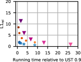
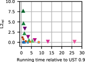
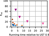
Figure 3: $\mathrm{L1}_{\mathrm{rel}}$, $\mathrm{L2}_{\mathrm{rel}}$ and $\mathrm{E}_{\mathrm{rel}}$ w. r. t. the running time of our algorithm with $\epsilon=0.9$. All data points are aggregated using the geometric mean over the instances of Table 2.

Figure 3 shows that, when assessing the error in terms of $\mathrm{L1}_{\mathrm{rel}}$, $\mathrm{L2}_{\mathrm{rel}}$, or $\mathrm{E}_{\mathrm{rel}}$, for the same running time UST yields results that are still better in terms of quality than the competitors’, but not by such a wide margin. This can be explained by the fact that the numerical solvers used by our competitors often employ measures analogous to $\mathrm{L1}_{\mathrm{rel}}$ and $\mathrm{L2}_{\mathrm{rel}}$ in their stopping conditions.

E.1 Parallel Scalability

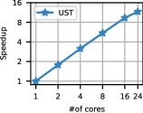
(a) Geometric mean of the speedup of UST on multiple cores (shared memory) w. r. t. a sequential run. Data points are aggregated over the instances of Tables 2 and 3 .

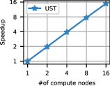
(b) Geometric mean of the speedup of UST on multiple compute nodes w. r. t. UST on a single compute node ($1\times 24$ cores). Data points are aggregated over the instances of Tables 2, 3, and 4 .

Figure 4: Parallel scalability of UST ($\epsilon=0.3$) with shared and with distributed memory.

Figures 4 and 5 report additional results regarding parallel scalability of UST.

E.2 Scalability on R-MAT Graphs

In Figure 6 we report additional results about the scalability of UST w. r. t. the graph size using the R-MAT [19] model. For this experiment we use the Graph500 parameter setting (i. e., edge factor 16, $a=0.57$, $b=0.19$, $c=0.19$, and $d=0.05$). The algorithm requires only $\numprint{18}$ minutes on inputs with up to $\numprint{134.2}$ million edges. In particular, since these graphs have a nearly-constant diameter, our algorithm is faster than on random hyperbolic graphs. Qualitatively, it exhibits a similar scalability.

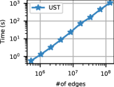
(a) Running time of UST w. r. t. #of edges.

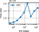
(b) Ratio of running time of UST w. r. t. its theoretical running time (see Theorem 3.3).

Figure 6: Scalability of UST on R-MAT graphs ($\epsilon=0.3$, $1\times 24$ cores).

E.3 Memory Consumption

Finally, we measure the peak memory consumption of all the algorithms while running sequentially on the instances of Tables 2 and 3. More precisely, we subtract the peak resident set size before launching the algorithm from the peak resident set size after the algorithm finished. Figure 7 shows that UST requires less memory than the competitors on all the considered instances. This can be explained by the fact that, unlike its competitors, our algorithm does not rely on Laplacian solvers with considerable memory overhead. For the largest network in particular, the peak memory is $\numprint{487.0}$ MB for UST, and at least $\numprint{1.6}$ GB for the competitors.

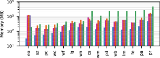
Figure 7: Difference between the peak resident set size before and after a sequential run of each algorithm on the instances of Tables 2 and 3.

E.4 Baseline

Table 6: Precision of the diagonal entries computed by the LAMG solver (tolerance: $10^{-9}$) compared with the ones computed by the Matlab pinv function.

Network Type $|V|$ |E| diam. $\max_{i}\mathbf{L}^{\dagger}_{ii}-\widetilde{\mathbf{L}^{\dagger}_{ii}}$ $\mathrm{E}_{\mathrm{rel}}$ $\mathrm{L1}_{\mathrm{rel}}$ $\mathrm{L2}_{\mathrm{rel}}$ Ranking moreno-lesmis characters 77 254 5 0,000 0 0,00% 0,00% 0,00% 0,48% petster-hamster-household social 874 4 003 8 0,000 6 0,23% 0,13% 0,07% 0,02% subelj-euroroad infrastructure 1 039 1 305 62 0,003 1 0,12% 0,09% 0,05% 0,00% arenas-email communication 1 133 5 451 8 0,000 2 0,13% 0,07% 0,03% 0,00% dimacs10-polblogs web 1 222 16 714 8 0,000 2 0,18% 0,07% 0,02% 0,01% maayan-faa infrastructure 1 226 2 408 17 0,000 5 0,08% 0,06% 0,03% 0,00% petster-hamster-friend social 1 788 12 476 14 0,000 3 0,15% 0,07% 0,02% 0,01% petster-hamster social 2 000 16 098 10 0,000 1 0,09% 0,04% 0,02% 0,01% wikipedia-link-lo web 3 733 82 977 9 0,000 1 0,05% 0,02% 0,01% 0,03% advogato social 5 042 39 227 9 0,000 1 0,03% 0,02% 0,01% 0,01% p2p-Gnutella06 computer 8 717 31 525 10 0,000 0 0,01% 0,01% 0,00% 0,00% p2p-Gnutella05 computer 8 842 31 837 9 0,000 1 0,02% 0,01% 0,01% 0,00%

References

- [1] David J. Aldous. The random walk construction of uniform spanning trees and uniform labelled trees. SIAM J. Discret. Math., 3(4):450–465, November 1990. doi:10.1137/0403039.
- [2] Vedat Levi Alev, Nima Anari, Lap Chi Lau, and Shayan Oveis Gharan. Graph clustering using effective resistance. In Anna R. Karlin, editor, 9th Innovations in Theoretical Computer Science Conference, ITCS 2018, January 11-14, 2018, Cambridge, MA, USA, volume 94 of LIPIcs, pages 41:1–41:16, Cambridge, Massachusetts, USA, 2018. Schloss Dagstuhl - Leibniz-Zentrum fuer Informatik. doi:10.4230/LIPIcs.ITCS.2018.41.
- [3] Patrick Amestoy, Iain S. Duff, Jean-Yves L’Excellent, and François-Henry Rouet. Parallel computation of entries of a. SIAM J. Scientific Computing, 37(2):C268–C284, 2015. doi:10.1137/120902616.
- [4] Eugenio Angriman, Maria Predari, Alexander van der Grinten, and Henning Meyerhenke. Approximation of the diagonal of a laplacian’s pseudoinverse for complex network analysis, 2020. arXiv:2006.13679.
- [5] Eugenio Angriman, Alexander van der Grinten, Moritz von Looz, Henning Meyerhenke, Martin Nöllenburg, Maria Predari, and Charilaos Tzovas. Guidelines for experimental algorithmics: A case study in network analysis. Algorithms, 12(7):127, 2019.
- [6] Haim Avron and Sivan Toledo. Randomized algorithms for estimating the trace of an implicit symmetric positive semi-definite matrix. J. ACM, 58(2):8:1–8:34, 2011. doi:10.1145/1944345.1944349.
- [7] David A Bader, Guojing Cong, and John Feo. On the architectural requirements for efficient execution of graph algorithms. In 2005 International Conference on Parallel Processing (ICPP’05), pages 547–556, Oslo, Norway, 2005. IEEE, IEEE.
- [8] Simon Barthelmé, Nicolas Tremblay, Alexandre Gaudillière, Luca Avena, and Pierre-Olivier Amblard. Estimating the inverse trace using random forests on graphs, 2019. arXiv:1905.02086.
- [9] C. Bekas, E. Kokiopoulou, and Y. Saad. An estimator for the diagonal of a matrix. Appl. Numer. Math., 57(11-12):1214–1229, November 2007. URL: http://dx.doi.org/10.1016/j.apnum.2007.01.003, doi:10.1016/j.apnum.2007.01.003.
- [10] Elisabetta Bergamini, Michele Borassi, Pierluigi Crescenzi, Andrea Marino, and Henning Meyerhenke. Computing top-k closeness centrality faster in unweighted graphs. TKDD, 13(5):53:1–53:40, 2019. doi:10.1145/3344719.
- [11] Elisabetta Bergamini, Michael Wegner, Dimitar Lukarski, and Henning Meyerhenke. Estimating current-flow closeness centrality with a multigrid laplacian solver. In Proc. 7th SIAM Workshop on Combinatorial Scientific Computing, CSC 2016, pages 1–12. SIAM, 2016. doi:10.1137/1.9781611974690.ch1.
- [12] Guy E. Blelloch, Anupam Gupta, Ioannis Koutis, Gary L. Miller, Richard Peng, and Kanat Tangwongsan. Near linear-work parallel sdd solvers, low-diameter decomposition, and low-stretch subgraphs, 2011. doi:10.1145/1989493.1989496.
- [13] Paolo Boldi and Sebastiano Vigna. Axioms for centrality. Internet Mathematics, 10(3-4):222–262, 2014. doi:10.1080/15427951.2013.865686.
- [14] Béla Bollobás. Modern Graph Theory, volume 184 of Graduate Texts in Mathematics. Springer, 2002. doi:10.1007/978-1-4612-0619-4.
- [15] Enrico Bozzo and Massimo Franceschet. Approximations of the generalized inverse of the graph laplacian matrix. Internet mathematics, 8(4):456–481, 2012.
- [16] Enrico Bozzo and Massimo Franceschet. Resistance distance, closeness, and betweenness. Social Networks, 35(3):460–469, 2013. doi:10.1016/j.socnet.2013.05.003.
- [17] Ulrik Brandes and Daniel Fleischer. Centrality measures based on current flow. In Proceedings of the 22nd Annual Symposium on Theoretical Aspects of Computer Science, STACS 2005, volume 3404 of LNCS, pages 533–544. Springer, 2005. URL: http://dx.doi.org/10.1007/978-3-540-31856-9_44, doi:10.1007/978-3-540-31856-9_44.
- [18] A. Broder. Generating random spanning trees. In Proceedings of the 30th Annual Symposium on Foundations of Computer Science, SFCS ’89, page 442–447, USA, 1989. IEEE Computer Society. doi:10.1109/SFCS.1989.63516.
- [19] Deepayan Chakrabarti, Yiping Zhan, and Christos Faloutsos. R-mat: A recursive model for graph mining. In Proceedings of the 2004 SIAM International Conference on Data Mining, pages 442–446. SIAM, SIAM, 2004.
- [20] Ashok K Chandra, Prabhakar Raghavan, Walter L Ruzzo, Roman Smolensky, and Prasoon Tiwari. The electrical resistance of a graph captures its commute and cover times. Computational Complexity, 6(4):312–340, 1996.
- [21] Michael B. Cohen, Rasmus Kyng, Gary L. Miller, Jakub W. Pachocki, Richard Peng, Anup B. Rao, and Shen Chen Xu. Solving sdd linear systems in nearly mlog1/2n time. In Proceedings of the Forty-Sixth Annual ACM Symposium on Theory of Computing, STOC ’14, page 343–352, New York, NY, USA, 2014. Association for Computing Machinery. doi:10.1145/2591796.2591833.
- [22] Wendy Ellens, Flora Spieksma, P. Mieghem, A. Jamakovic, and Robert Kooij. Effective graph resistance. Linear Algebra and its Applications, 435:2491–2506, 11 2011. doi:10.1016/j.laa.2011.02.024.
- [23] Josh Ericson, Pietro Poggi-Corradini, and Hainan Zhang. Effective resistance on graphs and the epidemic quasimetric. Involve, a Journal of Mathematics, 7(1):97–124, 2013.
- [24] Hutchinson M. F. A stochastic estimator of the trace of the influence matrix for laplacian smoothing splines. J. Commun. Statist. Simula., 19(2):433–450, 1990.
- [25] Arpita Ghosh, Stephen Boyd, and Amin Saberi. Minimizing effective resistance of a graph. SIAM Rev., 50(1):37–66, February 2008. URL: http://dx.doi.org/10.1137/050645452, doi:10.1137/050645452.
- [26] Chris Godsil and Gordon F Royle. Algebraic graph theory, volume 207. Springer Science & Business Media, 2013.
- [27] Gene H. Golub and Charles F. Van Loan. Matrix computations. Johns Hopkins University Press, 1996.
- [28] Gaël Guennebaud, Benoît Jacob, et al. Eigen v3. http://eigen.tuxfamily.org, 2010.
- [29] Takanori Hayashi, Takuya Akiba, and Yuichi Yoshida. Efficient algorithms for spanning tree centrality. In IJCAI, pages 3733–3739. IJCAI, 2016.
- [30] Mathias Jacquelin, Lin Lin, and Chao Yang. Pselinv – a distributed memory parallel algorithm for selected inversion: The non-symmetric case. Parallel Computing, 74:84 – 98, 2018. Parallel Matrix Algorithms and Applications (PMAA’16). URL: http://www.sciencedirect.com/science/article/pii/S0167819117301941, doi:https://doi.org/10.1016/j.parco.2017.11.009.
- [31] William B Johnson and Joram Lindenstrauss. Extensions of lipschitz mappings into a hilbert space. Contemporary mathematics, 26(189-206):1, 1984.
- [32] Jonathan A Kelner, Lorenzo Orecchia, Aaron Sidford, and Zeyuan Allen Zhu. A simple, combinatorial algorithm for solving sdd systems in nearly-linear time. In Proceedings of the forty-fifth annual ACM symposium on Theory of computing, pages 911–920. ACM, 2013.
- [33] Douglas Klein and Milan Randic. Resistance distance. Journal of Mathematical Chemistry, 12:81–95, 12 1993. doi:10.1007/BF01164627.
- [34] Ioannis Koutis, Gary L. Miller, and Richard Peng. A nearly-m log n time solver for SDD linear systems. In Rafail Ostrovsky, editor, IEEE 52nd Annual Symposium on Foundations of Computer Science, FOCS 2011, Palm Springs, CA, USA, October 22-25, 2011, pages 590–598. IEEE Computer Society, 2011. doi:10.1109/FOCS.2011.85.
- [35] Ioannis Koutis, Gary L. Miller, and Richard Peng. Approaching optimality for solving SDD linear systems. SIAM J. Comput., 43(1):337–354, 2014. URL: http://dx.doi.org/10.1137/110845914, doi:10.1137/110845914.
- [36] Ioannis Koutis, Gary L. Miller, and David Tolliver. Combinatorial preconditioners and multilevel solvers for problems in computer vision and image processing. Computer Vision and Image Understanding, 115(12):1638–1646, 2011.
- [37] Jérôme Kunegis. KONECT: the koblenz network collection. In Leslie Carr, Alberto H. F. Laender, Bernadette Farias Lóscio, Irwin King, Marcus Fontoura, Denny Vrandecic, Lora Aroyo, José Palazzo M. de Oliveira, Fernanda Lima, and Erik Wilde, editors, 22nd International World Wide Web Conference, WWW ’13, Rio de Janeiro, Brazil, May 13-17, 2013, Companion Volume, pages 1343–1350. International World Wide Web Conferences Steering Committee / ACM, 2013. doi:10.1145/2487788.2488173.
- [38] R. Kyng and S. Sachdeva. Approximate gaussian elimination for laplacians - fast, sparse, and simple. In 2016 IEEE 57th Annual Symposium on Foundations of Computer Science (FOCS), pages 573–582. IEEE, Oct 2016. doi:10.1109/FOCS.2016.68.
- [39] Rasmus Kyng, Yin Tat Lee, Richard Peng, Sushant Sachdeva, and Daniel A. Spielman. Sparsified cholesky and multigrid solvers for connection laplacians. In Proceedings of the Forty-Eighth Annual ACM Symposium on Theory of Computing, STOC ’16, page 842–850, New York, NY, USA, 2016. Association for Computing Machinery. doi:10.1145/2897518.2897640.
- [40] Huan Li, Richard Peng, Liren Shan, Yuhao Yi, and Zhongzhi Zhang. Current flow group closeness centrality for complex networks? In Ling Liu, Ryen W. White, Amin Mantrach, Fabrizio Silvestri, Julian J. McAuley, Ricardo Baeza-Yates, and Leila Zia, editors, The World Wide Web Conference, WWW 2019, San Francisco, CA, USA, May 13-17, 2019, pages 961–971. ACM, 2019. doi:10.1145/3308558.3313490.
- [41] Huan Li and Zhongzhi Zhang. Kirchhoff index as a measure of edge centrality in weighted networks: Nearly linear time algorithms. In Proceedings of the Twenty-Ninth Annual ACM-SIAM Symposium on Discrete Algorithms, pages 2377–2396. SIAM, SIAM, 2018.
- [42] Oren E Livne and Achi Brandt. Lean algebraic multigrid (LAMG): Fast graph laplacian linear solver. SIAM Journal on Scientific Computing, 34(4):B499–B522, 2012.
- [43] L. Lovász. Random walks on graphs: A survey. In D. Miklós, V. T. Sós, and T. Szőnyi, editors, Combinatorics, Paul Erdős is Eighty, volume 2, pages 353–398. János Bolyai Mathematical Society, Budapest, 1996.
- [44] Andrew Lumsdaine, Douglas Gregor, Bruce Hendrickson, and Jonathan Berry. Challenges in parallel graph processing. Parallel Processing Letters, 17(01):5–20, 2007.
- [45] Russell Lyons and Yuval Peres. Probability on Trees and Networks. Cambridge University Press, USA, 1st edition, 2017.
- [46] Clémence Magnien, Matthieu Latapy, and Michel Habib. Fast computation of empirically tight bounds for the diameter of massive graphs. Journal of Experimental Algorithmics (JEA), 13:1–10, 2009.
- [47] Charalampos Mavroforakis, Richard Garcia-Lebron, Ioannis Koutis, and Evimaria Terzi. Spanning Edge Centrality: Large-scale Computation and Applications. In Proceedings of the 24th International Conference on World Wide Web, WWW 2015, pages 732–742. ACM, 2015.
- [48] Brendan D McKay et al. Practical graph isomorphism. Department of Computer Science, Vanderbilt University Tennessee, USA, 1981.
- [49] Onuttom Narayan and Iraj Saniee. Scaling of random walk betweenness in networks. In Luca Maria Aiello, Chantal Cherifi, Hocine Cherifi, Renaud Lambiotte, Pietro Lió, and Luis M. Rocha, editors, Complex Networks and Their Applications VII, pages 41–51, Cham, 2019. Springer International Publishing.
- [50] Mark Newman. Networks (2nd Ed.). Oxford university press, 2018.
- [51] Kazuya Okamoto, Wei Chen, and Xiang-Yang Li. Ranking of closeness centrality for large-scale social networks. In International workshop on frontiers in algorithmics, pages 186–195. Springer, Springer, 2008.
- [52] Melissa E. O’Neill. Pcg: A family of simple fast space-efficient statistically good algorithms for random number generation. Technical Report HMC-CS-2014-0905, Harvey Mudd College, Claremont, CA, September 2014.
- [53] Richard Peng and Daniel A. Spielman. An efficient parallel solver for sdd linear systems, 2014. doi:10.1145/2591796.2591832.
- [54] Gyan Ranjan, Zhi-Li Zhang, and Daniel Boley. Incremental computation of pseudo-inverse of laplacian. In Zhao Zhang, Lidong Wu, Wen Xu, and Ding-Zhu Du, editors, Combinatorial Optimization and Applications, pages 729–749, Cham, 2014. Springer International Publishing.
- [55] Aaron Schild. An almost-linear time algorithm for uniform random spanning tree generation. In Proceedings of the 50th Annual ACM SIGACT Symposium on Theory of Computing, STOC 2018, page 214–227, New York, NY, USA, 2018. Association for Computing Machinery. doi:10.1145/3188745.3188852.
- [56] John Shawe-Taylor and Nello Cristianini. Kernel Methods for Pattern Analysis. Cambridge University Press, USA, 2004.
- [57] Jack Sherman and Winifred J. Morrison. Adjustment of an inverse matrix corresponding to a change in one element of a given matrix. Ann. Math. Statist., 21(1):124–127, 03 1950.
- [58] Roger B. Sidje and Yousef Saad. Rational approximation to the fermi-dirac function with applications in density functional theory. Numerical Algorithms, 56(3):455–479, 3 2011. doi:10.1007/s11075-010-9397-6.
- [59] Daniel A. Spielman and Nikhil Srivastava. Graph sparsification by effective resistances. SIAM Journal on Computing, 40(6):1913–1926, 2011. URL: http://dx.doi.org/10.1137/080734029, doi:10.1137/080734029.
- [60] Christian L. Staudt, Aleksejs Sazonovs, and Henning Meyerhenke. Networkit: A tool suite for large-scale complex network analysis. Network Science, 4(4):508–530, 2016. doi:10.1017/nws.2016.20.
- [61] Jok M. Tang and Yousef Saad. A probing method for computing the diagonal of a matrix inverse. Numerical Linear Algebra with Applications, 19(3):485–501, 2012.
- [62] Piet Van Mieghem, Karel Devriendt, and H Cetinay. Pseudoinverse of the laplacian and best spreader node in a network. Physical Review E, 96(3):032311, 2017.
- [63] Moritz von Looz, Mustafa Safa Özdayi, Sören Laue, and Henning Meyerhenke. Generating massive complex networks with hyperbolic geometry faster in practice. In 2016 IEEE High Performance Extreme Computing Conference, HPEC 2016, Waltham, MA, USA, September 13-15, 2016, pages 1–6. IEEE, 2016. doi:10.1109/HPEC.2016.7761644.
- [64] David Bruce Wilson. Generating random spanning trees more quickly than the cover time. In Proceedings of the Twenty-eighth Annual ACM Symposium on Theory of Computing, STOC ’96, pages 296–303, New York, NY, USA, 1996. ACM. URL: http://doi.acm.org/10.1145/237814.237880, doi:10.1145/237814.237880.