Thermal Stability of Superconductors

Abstract

A stability criterion is worked out for the superconducting phase. The validity of a prerequisite, established previously for persistent currents, is thereby confirmed. Temperature dependence is given for the specific heat and concentration of superconducting electrons in the vicinity of the critical temperature $T_{c}$. The isotope effect, mediated by electron-phonon interaction and hyperfine coupling, is analyzed. Several experiments, intended at validating this analysis, are presented, including one giving access to the specific heat of high-$T_{c}$ compounds.

I Introduction

In the mainstream viewpar ; sch ; tin , the thermal properties of superconductors are discussed within the framework of the phenomenological equation by Ginzburg and Landaugin (GL) and the BCS theorybcs . However, since this work is aimed at accounting for the stability of the superconducting state with respect to the normal one, we shall develope an alternative approach, based on thermodynamicslan , the properties of the Fermi gasash and recent resultssz5 ; sz4 , claimed to be valid for all superconductors, including low and high $T_{c}$ materials.

The outline is as follows : the specific heat of the superconducting phase is calculated in section $2$, which enables us to assess its binding energy and thereby to confirm and refine a necessary condition, established previously for the existence of persistent currentssz4 ; section $3$ is concerned with the inter-electron coupling, mediated by the electron-phonon and hyperfine interactions; new experiments, dedicated at validating this analysis, are discussed in section $4$ and the results are summarised in the conclusion.

II Binding Energy

As in our previous worksz4 ; sz5 ; sz1 ; sz2 ; sz3 ; sz7 , the present analysis will proceed within the framework of the two-fluid model, for which the conduction electrons comprise bound and independent electrons, in respective temperature dependent concentration $c_{s}(T),c_{n}(T)$. They are organized, respectively, as a many bound electronsz5 (MBE) state, characterised by its chemical potential $\mu(c_{s})$, and a Fermi gasash of Fermi energy $E_{F}(T,c_{n})$. The Helmholz free energy of independent electrons per unit volume $F_{n}$ and $E_{F}$ on the one hand, and the eigenenergy per unit volume $\mathcal{E}_{s}(c_{s})$ of bound electrons and $\mu$ on the other hand, are relatedash ; lan , respectively, by $E_{F}=\frac{\partial F_{n}}{\partial c_{n}}$ and $\mu=\frac{\partial\mathcal{E}_{s}}{\partial c_{s}}$. At last, according to Gibbs and Duhem’s lawlan , the two-fluid model fulfilssz4 at thermal equilibrium

$$E_{F}(T,c_{n}(T))=\mu(c_{s}(T)),\quad c_{0}=c_{s}(T)+c_{n}(T),$$ (1)

with $c_{0}$ being the total concentration of conduction electrons. Solutions of Eq.(1) are given for $T=0,T_{c}$ in Fig.1. Besides, Eq.(1) has been shownsz5 ; sz4 to read for $T=T_{c}$ (see $B$ in Fig.1)

$$E_{F}(T_{c},c_{0})=\mu(c_{s}=0)=\varepsilon_{c}/2\quad,$$ (2)

with $\varepsilon_{c}$ being the energy of a bound electron pairsz5 . Note that Eq.(2) is consistent with the superconducting transition, occuring at $T_{c}$, being of second orderlan , whereas it has been shownsz5 to be of first order at $T<T_{c}$, if the sample is flown through by a finite current. Then the binding energy of the superconducting state $E_{b}(T<T_{c})$ has been workedsz5 ; gor out as

$$E_{b}(T)=\int_{T}^{T_{c}}\left(C_{s}(u)-C_{n}(u)\right)du\quad,$$ (3)

with $C_{s}(T),C_{n}(T)=\frac{\left(\pi k_{B}\right)^{2}}{3}\rho(E_{F})T,$ being the electronic specific heat of a superconductor, flown through by a vanishing currentsz5 and that of a degenerate Fermi gasash ($k_{B},\rho(E_{F})$ stand for Boltzmann’s constant and the one-electron density of states at the Fermi energy). Due to Eq.(3), a stable superconducting phase $\Leftrightarrow E_{b}>0$ requires $C_{s}(T)>C_{n}(T)$, which is confirmed experimentallypar ; ash , namely $C_{s}(T_{c})\approx 3C_{n}(T_{c})$.

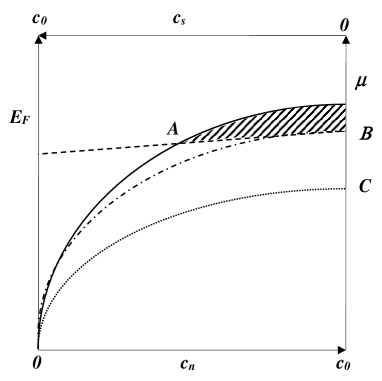
Figure 1: Schematic plots of $E_{F}(T=0,c_{n})$, $E_{F}(T_{c},c_{n})$, $E_{F}(T>T_{c},c_{n})$ and $\mu(c_{s})$ as solid, dashed-dotted, dotted and dashed lines, respectively; $\frac{\partial\mu}{\partial c_{s}}$ has been taken to be constant for simplicity; the origin $E_{F}=\mu=0$ is set at the bottom of the conduction band; the crossing points $A,B$ of $E_{F}(0,c_{n}),E_{F}(T_{c},c_{n})$, respectively, with $\mu(c_{s})$, exemplify stable solutions of Eq.(1); the tiny differences $E_{F}(T,c_{n})-\mu(c_{0}-c_{n})$ have been hugely magnified for the reader’s convenience.

The bound and independent electrons contribute, respectively,

$$\begin{array}[]{l}\mathcal{E}_{s}(c_{s})=\int_{0}^{c_{s}}\mu(u)du\\ \mathcal{E}_{n}(T,c_{n})=\int_{\epsilon_{b}}^{\epsilon_{u}}\epsilon\rho(\epsilon)f(\epsilon-E_{F},T)d\epsilon\end{array}\quad,$$

to the total electronic energy $\mathcal{E}=\mathcal{E}_{n}+\mathcal{E}_{s}$. The symbols $\epsilon,f(\epsilon-E_{F},T)$ refer to the one-electron energy and Fermi-Dirac distribution, while $\epsilon_{b},\epsilon_{u}$ designate the lower and upper limits of the conduction band. Then, thanks to Eq.(1) ($\Rightarrow dc_{n}+dc_{s}=dE_{F}-d\mu=0$), $C_{s}(T)=\frac{d\mathcal{E}}{dT}$ is inferred to read

$$C_{s}=\frac{\partial\mathcal{E}_{n}}{\partial T}-E_{F}\frac{\partial c_{n}}{\partial T}+\frac{dE_{F}}{dT}\left(\frac{\partial\mathcal{E}_{n}}{\partial E_{F}}-E_{F}\frac{\partial c_{n}}{\partial E_{F}}\right)\quad,$$ (4)

with $c_{n}=c_{n}(T),c_{s}=c_{s}(T),E_{F}=E_{F}\left(T,c_{n}(T)\right)$. Because the independent electrons make up a degenerate Fermi gas ($\Rightarrow T<<T_{F}=E_{F}/k_{B}$), the following expressions can be obtained owing to the Sommerfeld expansionash up to $T^{2}$

$$\begin{array}[]{c}\frac{\partial\mathcal{E}_{n}}{\partial E_{F}}=E_{F}\rho+\left(2\rho^{\prime}+E_{F}\rho^{\prime\prime}\right)\frac{\left(\pi k_{B}T\right)^{2}}{6}\\ \frac{\partial\mathcal{E}_{n}}{\partial T}=\left(\rho+E_{F}\rho^{\prime}\right)\frac{\left(\pi k_{B}\right)^{2}}{3}T\\ \frac{\partial c_{n}}{\partial E_{F}}=\rho+\rho^{\prime\prime}\frac{\left(\pi k_{B}T\right)^{2}}{6}\quad,\quad\frac{\partial c_{n}}{\partial T}=\rho^{\prime}\frac{\left(\pi k_{B}\right)^{2}}{3}T\end{array}\quad,$$ (5)

with $\rho=\rho(E_{F}),\rho^{\prime}=\frac{d\rho}{dE_{F}}(E_{F}),\rho^{\prime\prime}=\frac{d^{2}\rho}{dE_{F}^{2}}(E_{F})$. Then Eq.4 is finally recast into

$$C_{s}(T)=\frac{\left(\pi k_{B}\right)^{2}}{3}\rho T\left(1+\frac{dE_{F}}{dT}\frac{\rho^{\prime}}{\rho}T\right)\quad.$$ (6)

Applying Eq.6 at $T=T_{c}$ yields

$$C_{s}(T_{c})=C_{n}(T_{c})\left(1+\frac{dE_{F}}{dT}(T_{c}^{-})\frac{\rho^{\prime}}{\rho}T_{c}\right)\quad.$$ (7)

Hence it is in order to work out the expressions of $\frac{dE_{F}}{dT}(T>T_{c})$ and $\frac{dE_{F}}{dT}(T\leq T_{c})$.

Due to $c_{n}(T>T_{c})=c_{0}$, $\frac{dE_{F}}{dT}$ is deducedash to read

$$\frac{dE_{F}}{dT}(T>T_{c})=-\frac{\frac{\partial c_{n}}{\partial T}}{\frac{\partial c_{n}}{\partial E_{F}}}=-\frac{\left(\pi k_{B}\right)^{2}}{3}\frac{\rho^{\prime}}{\rho}T\quad,$$ (8)

which is integrated with respect to $T$ to yield

$$E_{F}(T=0,c_{0})-E_{F}(T,c_{0})=\frac{\left(\pi k_{B}\right)^{2}}{6}\frac{\rho^{\prime}}{\rho}T^{2}\quad.$$ (9)

Then consistency with Fig.1 requires $\rho^{\prime}(E_{F})>0$ so that $C$ goes toward $B$ for $T\searrow T_{c}$. Assuming $\rho(\epsilon)=\rho_{f}(\epsilon)\propto\sqrt{\epsilon}\Rightarrow\rho_{f}^{\prime}(\epsilon)>0,\forall\epsilon$, with $\rho_{f}(\epsilon)$ being the density of states of three-dimensional free electrons, leads to

$$1-\frac{E_{F}(T>T_{c})}{E_{F}(0,c_{0})}=\frac{\pi^{2}}{12}\left(\frac{T}{T_{F}}\right)^{2}\quad.$$

A numerical application with a typical value $T_{F}=3\times 10^{4}K$ yields $T_{F}(300K)-T_{F}(0)\approx 3K<<T_{F}\Rightarrow\left|\frac{dT_{F}}{dT}\left(T>T_{c}\right)\right|<<1$.

Taking advantage of Eq.1, the expression of $\frac{dE_{F}}{dT}(T\leq T_{c})$ is obtained to read

$$\left.\begin{array}[]{l}dc_{n}=\frac{\partial c_{n}}{\partial E_{F}}dE_{F}+\frac{\partial c_{n}}{\partial T}dT\\ dc_{s}=\frac{\partial c_{s}}{\partial\mu}d\mu=-dc_{n}\end{array}\right\}\Rightarrow\frac{dE_{F}}{dT}=-\frac{\frac{\partial c_{n}}{\partial T}}{\beta(T)}\quad,$$ (10)

with $\beta(T)=\frac{\partial c_{n}}{\partial E_{F}}+\frac{\partial c_{s}}{\partial\mu}$. The Sommerfeld expansion (see Eq.(5)) leads to

$$\alpha=\frac{dE_{F}}{dT}(T_{c}^{-})\frac{\rho^{\prime}}{\rho}T_{c}=-\frac{\left(\pi k_{B}\rho^{\prime}T_{c}\right)^{2}}{3\rho\beta(T_{c})}\quad.$$ (11)

Thus, looking back at Eq.7, it is realized that the observedpar ; ash relation $C_{s}(T_{c})\approx 3C_{n}(T_{c})$ requires $\alpha>0\Rightarrow\beta(T_{c})<0$, which had been already identifiedsz4 as a necessary condition for the superconducting state to be at thermal equilibrium. At last, $\alpha$ reads in case of $\rho=\rho_{f}$

$$\alpha=\frac{\pi^{2}}{12}\left(\frac{T}{T_{F}}\right)^{2}\rho\frac{\partial E_{F}}{\partial c_{n}}\left(1+\frac{\partial E_{F}}{\partial c_{n}}\frac{\partial c_{s}}{\partial\mu}\right)^{-1}\quad.$$

Due to $\frac{T}{T_{F}}<<1$ and $\rho\frac{\partial E_{F}}{\partial c_{n}}\approx 1$, getting $\alpha\approx 2$ requires $\beta(T_{c})\approx 0\Rightarrow\frac{\partial E_{F}}{\partial c_{n}}+\frac{\partial\mu}{\partial c_{s}}\approx 0$, so that the stability criterion of the superconducting state reads finally

$$\frac{\partial E_{F}}{\partial c_{n}}(T_{c},c_{0})=-\frac{\partial\mu}{\partial c_{s}}(0),\quad\rho^{\prime}(E_{F}(T_{c},c_{0}))>0\quad.$$ (12)

Because of $\frac{\partial E_{F}}{\partial c_{n}}(T_{c},c_{0})\approx\frac{1}{\rho}>0$, Eq.(12) is seen to be consistent with $\frac{\partial\mu}{\partial c_{s}}(c_{s})<0$, established previously as a prerequisite for persistent currentssz4 and the Josephson effectsz6 . At last, note that there is $\frac{dT_{F}}{dT}(T\leq T_{c})>>1$ but inversely $0<-\frac{dT_{F}}{dT}(T>T_{c})<<1$.

In order to grasp the significance of the constraint expressed by Eq.(12), let us elaborate the case for which Eq.(12) is not fulfilled ($\Rightarrow C_{s}(T<T_{c})<C_{n}(T)$). Accordingly the hatched area in Fig.1 is equal to the difference in free energy at $T=0$ between the superconducting phase and the normal one, and thence also equal to $E_{b}(0)>0$ because the entropy of the normal state vanisheslan at $T=0$. However applying Eq.(3) with $C_{s}(T<T_{c})<C_{n}(T)$ yields $E_{b}(0)<0$, which contradicts the above opposite conclusion $E_{b}(0)>0$, and thereby entails that the MBE state, associated with $A$ in Fig.1, is not observable at thermal equilibrium in case of unfulfilled Eq.(12), even though it is definitely a MBE eigenstateja1 ; ja2 ; ja3 of the Hubbard Hamiltonian, accounting for the motion of correlated electrons, and its energy is indeed lower than that of the Fermi gas $\mathcal{E}_{n}(T=0,c_{0})$.

Since energy and free energy are equallan at $T=0$, $E_{b}(0)$ reads

$$E_{b}(0)=\int_{0}^{c_{s}(0)}\left(E_{F}(0,c_{0}-c_{s})-\mu(c_{s})\right)dc_{s}\quad.$$

In order to work out an upper bound for $E_{b}(0)$, $E_{F}(T,c_{0}-c_{s})-\mu(c_{s})$ will be approximated by its Taylor expansion at first order with respect to $c_{s}-c_{s}(T)$, which yields

$$E_{F}(T,c_{0}-c_{s})-\mu(c_{s})\approx\frac{m}{e^{2}}\gamma\left(c_{s}(T)-c_{s}\right)\quad,$$ (13)

with $\gamma=\frac{\partial E_{F}}{\partial c_{n}}(c_{n}(T))+\frac{\partial\mu}{\partial c_{s}}(c_{s}(T))$. Since it has been shownsz5 that $E_{F}(T,c_{0}-c_{s})-\mu(c_{s})<10^{-5}eV$, Eq.(13) turns out to be very accurate. Likewise, due to $c_{s}(T)\geq c_{s}\geq 0$ (see Fig.1) and $\gamma>0$ being a necessary conditionsz4 for $A$ in Fig.1 to correspond to a stable equilibrium, Eq.(13) entails

$$E_{F}(T,c_{0}-c_{s})-\mu(c_{s})\leq E_{F}(T,c_{0})-\mu(0)\quad.$$

Then by taking advantage of Eqs.(2,9), we get

$$E_{F}(T,c_{0})-\mu(0)\leq E_{F}(0,c_{0})-E_{F}(T_{c},c_{0})=\frac{\left(\pi k_{B}T_{c}\right)^{2}}{6}\frac{\rho^{\prime}}{\rho},$$

with $\rho^{\prime}>0$ as required by Eq.(12). At last, assuming $\rho(\epsilon)=\rho_{f}(\epsilon)$, the searched upper bound per electron is obtained to read

$$\frac{E_{b}(0)}{c_{0}E_{F}(T_{c},c_{0})}\leq\frac{\pi^{2}}{12}\left(\frac{T_{c}}{T_{F}}\right)^{2}\quad.$$

Applying this formula to $Al$ ($T_{c}=1.2K,T_{F}\approx 3\times 10^{4}K$) gives $\frac{E_{b}(0)}{c_{0}E_{F}(T_{c},c_{0})}<10^{-8}$. Moreover, that latter result had enabled us to realizesz2 that the formula $E_{b}(0)=\mu_{0}H_{c}(0)^{2}/2$, albeit ubiquitous in textbookspar ; sch ; tin ($H_{c}(T\leq T_{c}),\mu_{0}$ refer to the critical magnetic field and the magnetic permeability of vacuum, respectively), underestimates $E_{b}(0)$ by ten orders of magnitude.

Since fulfilling Eq.(12) is tantamount to $\beta(T_{c})=0$, which entails $\frac{dE_{F}}{dT}(T\rightarrow T_{c}^{-})\rightarrow\infty$ and thence $C_{s}(T\rightarrow T_{c}^{-})\rightarrow\infty$, it must be checked that $\mathcal{E}(T)=\int_{0}^{T}C_{s}(u)du$ remains still finite for $T\rightarrow T_{c}^{-}$. To that end, let us work out the Taylor expansion of $\mu(c_{s}),E_{F}(T,c_{n})$ up to the second order around $T=0,c_{s}=0$

$$\begin{array}[]{l}\mu(c_{s})=\mu(0)+\frac{\partial\mu}{\partial c_{s}}(0)c_{s}+\frac{\partial^{2}\mu}{\partial c_{s}^{2}}(0)\frac{c_{s}^{2}}{2}\\ E_{F}(T,c_{n})=E_{F}(T_{c},c_{0})-\frac{c_{s}}{\rho}-\frac{\rho^{\prime}}{\rho^{3}}\frac{c_{s}^{2}}{2}\\ \quad\quad\quad\quad\quad+\frac{\left(\pi k_{B}\right)^{2}}{6}\frac{\rho^{\prime}}{\rho}\left(T_{c}^{2}-T^{2}\right)\end{array}\quad,$$

for which we have used $c_{n}=c_{0}-c_{s},c_{s}=c_{s}(T),\frac{\partial E_{F}}{\partial c_{n}}=\frac{1}{\rho}\Rightarrow\frac{\partial^{2}E_{F}}{\partial c_{n}^{2}}=-\frac{\rho^{\prime}}{\rho^{3}}$. Then taking advantage of Eqs.(1,2) ($\Rightarrow E_{F}(T,c_{n})=\mu(c_{s}),E_{F}(T_{c},c_{0})=\mu(0)$) and Eq.(12) ($\Rightarrow\beta(T_{c})=\frac{\partial\mu}{\partial c_{s}}(0)+\frac{1}{\rho}=0$) results into

$$c_{s}(T\rightarrow T_{c}^{-})=\pi k_{B}\sqrt{\frac{\rho^{\prime}\left(T_{c}^{2}-T^{2}\right)}{3\left(\rho\frac{\partial^{2}\mu}{\partial c_{s}^{2}}(0)+\frac{\rho^{\prime}}{\rho^{2}}\right)}}\propto\sqrt{T_{c}-T}\quad.$$

It should be noticed that the GL equation predictstin rather $c_{s}(T\rightarrow T_{c}^{-})\propto T_{c}-T$.

Likewise, let us calculate similarly the Taylor expansion of $\beta(T)\propto\frac{\partial E_{F}}{\partial c_{n}}+\frac{\partial\mu}{\partial c_{s}}$ up to the first order around $T=T_{c},c_{s}=0$

$$\begin{array}[]{c}\beta(T\rightarrow T_{c}^{-})\propto\left(\frac{\partial^{2}\mu}{\partial c_{s}^{2}}(0)-\frac{\partial^{2}E_{F}}{\partial c_{n}^{2}}(T_{c},c_{0})\right)c_{s}\Rightarrow\\ \beta(T\rightarrow T_{c}^{-})\propto\sqrt{T_{c}-T}\Rightarrow\mathcal{E}(T\rightarrow T_{c}^{-})\propto\sqrt{T_{c}-T}\end{array}\quad,$$

whence $\mathcal{E}(T\rightarrow T_{c}^{-})$ is concluded to remain indeed finite.

At last, we shall work out the expression of $j_{M}(T\rightarrow T_{c}^{-})$, the maximum current density $j_{s}$, conveyed by bound electrons which was shownsz5 to read

$$j_{M}=ec_{m}(T)\sqrt{\frac{2}{m}\left(E_{F}\left(T,c_{0}-c_{m}(T)\right)-\mu(c_{m}(T))\right)}\quad,$$

with $e,m$ standing for the charge and effective mass of the electron, while $c_{m}(T)=\frac{2}{3}c_{s}(T)$ designates the corresponding value of $c_{s}$, i.e. $j_{s}(c_{m})=j_{M}$. Hence $j_{M}$ readssz5 finally

$$\begin{array}[]{c}j_{M}(T)=\frac{er}{\sqrt{m}}\left(\frac{2}{3}c_{s}(T)\right)^{1.5}\\ r=\sqrt{\frac{\partial E_{F}}{\partial c_{n}}(c_{n}(T))+\frac{\partial\mu}{\partial c_{s}}(c_{s}(T))}\end{array}\quad.$$

It ensues from $\beta(T_{c})=0$ that the leading term of the Taylor expansion of $r$ around $T=T_{c},c_{s}=0$ reads

$$\begin{array}[]{c}r\left(T\rightarrow T_{c}^{-}\right)\propto\sqrt{c_{s}(T)}\Rightarrow r\propto\left(T_{c}-T\right)^{\frac{1}{4}}\Rightarrow\\ j_{M}\left(T\rightarrow T_{c}^{-}\right)\propto T_{c}-T\end{array}\quad,$$

which is to be compared with the maximum persistent current densitysz5 $j_{c}\left(T\rightarrow T_{*}^{-}\right)\propto\sqrt{T_{*}-T}$ with $T_{*}<T_{c}$.

III Isotope Effect

Substituting, in a superconducting material, an atomic species of mass $M$ by an isotope, is well-knownpar ; sch ; tin to alter $T_{c}$. This isotope effect was ascribed to the electron-phonon coupling, on the basis of the observed relation $T_{c}\sqrt{M}=constant$. The ensueing theoretical treatmentpar ; sch ; tin capitalisedfro on Froehlich’s perturbationlan2 calculation of the self-energy of an independent electron induced by the electron-phonon coupling. However since the BCS picturebcs has subsequently ascertained the paramount role of inter-electron coupling, we shall rather focus hereafter on the effective phonon-mediated interaction between two electrons.

Thus let us consider independent electrons of spin $\sigma=\pm 1/2$, moving in a three-dimensional crystal, containing $N$ sites. The dispersion of the one-electron band reads $\epsilon(k)$ with $\epsilon(k),k$ being the electron, spin-independent ($\Rightarrow\epsilon(-k)=\epsilon(k)$) energy and a vector of the Brillouin zone, respectively. Their motion is governed, in momentum space, by the Hamiltonian $H_{d}$

$$H_{d}=\sum_{k,\sigma}\epsilon(k)c^{+}_{k,\sigma}c_{k,\sigma}\quad,$$

with the sum over $k$ to be carried out over the whole Brillouin zone. Then the $c^{+}_{k,\sigma},c_{k,\sigma}$’s are Fermi-like creation and annihilation operatorssch on the Bloch state $\left|k,\sigma\right\rangle$

$$\left|k,\sigma\right\rangle=c^{+}_{k,\sigma}\left|0\right\rangle\quad,\quad\left|0\right\rangle=c_{k,\sigma}\left|k,\sigma\right\rangle\quad,$$

with $\left|0\right\rangle$ being the no electron state. Let us introduce now the electron-phononpar ; sch ; tin ; fro coupling $h_{e-\phi}$

$$h_{e-\phi}=\frac{g_{q}}{\sqrt{N}}\sum_{k,k^{\prime},\sigma}c^{+}_{k,\sigma}c_{k^{\prime},\sigma}\left(a^{+}_{q}+a_{-q}\right)\quad,$$

with $q=k^{\prime}-k$ and $g_{q}\propto\left(\omega_{q}M\right)^{-1/2}$ being the coupling constant characterising the electron-phonon interaction. Likewise, $\omega_{q}$ is the phonon frequency, while the $a^{+}_{q},a_{q}$’s are Bose-like creation and annihilation operatorssch on the $n_{q}\in\mathcal{N}$ phonon state $\left|n_{q}\right\rangle$

$$a^{+}_{q}\left|n_{q}\right\rangle=\sqrt{n_{q}+1}\left|n_{q}+1\right\rangle\quad,\quad a_{q}\left|n_{q}\right\rangle=\sqrt{n_{q}}\left|n_{q}-1\right\rangle.$$

Because of $\left\langle k\left|h_{e-\phi}\right|k^{\prime}\right\rangle=0,\forall k,k^{\prime}$ with $\left.|k\right\rangle=c^{+}_{k,+}c^{+}_{-k,-}\left.|0\right\rangle,\left.|k^{\prime}\right\rangle=c^{+}_{k^{\prime},+}c^{+}_{-k^{\prime},-}\left.|0\right\rangle$, we shall deal with $h_{e-\phi}$ as a perturbation with respect to $H_{d}$, in order to reckon $\left\langle k\left|k^{\prime}_{2}\right.\right\rangle$ with $\left|k^{\prime}_{2}\right\rangle$ denoting $\left|k^{\prime}\right\rangle$ perturbed at second orderlan2 . Accordingly, we first introduce the unperturbed electron-phonon eigenstates

$$\left|\widetilde{k}\right\rangle=\left|k\right\rangle\otimes\frac{\left|n_{q}\right\rangle+\left|n_{-q}\right\rangle}{\sqrt{2}},\quad\left|\widetilde{k^{\prime}}\right\rangle=\left|k^{\prime}\right\rangle\otimes\frac{\left|n_{q}\right\rangle+\left|n_{-q}\right\rangle}{\sqrt{2}}\quad,$$

with $n_{q}=n_{-q}=n$. Their respective energies read $E(k)=2\epsilon(k)+n\hbar\omega_{q}$, $E(k^{\prime})=2\epsilon(k^{\prime})+n\hbar\omega_{q}$. Then we reckon $\left|\widetilde{k^{\prime}_{2}}\right\rangle$ and further project it onto $\left|\widetilde{k}\right\rangle$, which yields

$$\begin{array}[]{l}\left\langle\widetilde{k}\left|\widetilde{k^{\prime}_{2}}\right.\right\rangle=\frac{g^{2}_{q}}{2N}\left(\left\langle\widetilde{k}\left|h_{e-\phi}\right|\varphi_{+}\right\rangle\left\langle\varphi_{+}\left|h_{e-\phi}\right|\widetilde{k^{\prime}}\right\rangle\right.\\ \quad\quad\quad\quad\quad\quad\left.+\left\langle\widetilde{k}\left|h_{e-\phi}\right|\varphi_{-}\right\rangle\left\langle\varphi_{-}\left|h_{e-\phi}\right|\widetilde{k^{\prime}}\right\rangle\right)\\ \varphi_{+}=c^{+}_{k,+}c^{+}_{-k^{\prime},-}\left|0\right\rangle\otimes\left(\frac{\sqrt{n+1}}{D_{+}}\left|n_{q}+1\right\rangle+\frac{\sqrt{n}}{D_{-}}\left|n_{-q}-1\right\rangle\right)\\ \varphi_{-}=c^{+}_{k^{\prime},+}c^{+}_{-k,-}\left|0\right\rangle\otimes\left(\frac{\sqrt{n+1}}{D_{+}}\left|n_{-q}+1\right\rangle+\frac{\sqrt{n}}{D_{-}}\left|n_{q}-1\right\rangle\right)\end{array},$$

with $D_{\pm}=\epsilon_{k}-\epsilon_{k^{\prime}}\pm\hbar\omega_{q}$. The searched $x_{k,k^{\prime}}=N\left\langle k\left|k^{\prime}_{2}\right.\right\rangle$ is then inferred to read

$$x_{k,k^{\prime}}=\frac{\left(2n(T)+1\right)g^{2}_{q}}{\left(\left(\epsilon_{k}-\epsilon_{k^{\prime}}\right)^{2}-\left(\hbar\omega_{q}\right)^{2}\right)}\quad,$$

with $n(T)=\left(e^{\frac{\hbar\omega_{q}}{k_{B}T}}-1\right)^{-1}$ being the thermal average of $n_{\pm q}$. Moreover it can be checked that $x_{k,k^{\prime}}=x_{k^{\prime},k}$. Thus, for $q$ not close to the Brillouin zone center (the most likely occurence), there is $x_{k,k^{\prime}}>0$, whereas $x_{k,k^{\prime}}<0$ can be found only for $q\approx 0$. Likewise, though the hereabove expression is redolent of one derived by Froehlichfro , their respective significances are unrelated, since Froehlich interpreted the self-energy of one electron and one phonon bound together in terms of virtual transitions between various electron-phonon states, whereas $x_{k,k^{\prime}}$ refers to the dot product of two-electron-states.

Projecting the hermitian BCS Hamiltonianbcs ; ja1 ; ja2 ; ja3 $H$ onto the basis $\left\{\left|k_{2}\right\rangle,\left|k^{\prime}_{2}\right\rangle\right\}$ yields

$$\begin{array}[]{l}H_{k_{2},k_{2}}=2\left(\epsilon_{k}+\frac{x_{k,k^{\prime}}U}{N^{2}}+\frac{x^{2}_{k,k^{\prime}}}{N^{2}}\epsilon_{k^{\prime}}\right)\\ H_{k_{2},k^{\prime}_{2}}=\frac{U}{N}\left(1+\frac{x^{2}_{k,k^{\prime}}}{N^{2}}\right)+2\frac{x_{k,k^{\prime}}}{N}\left(\epsilon_{k}+\epsilon_{k^{\prime}}\right)\\ H_{k^{\prime}_{2},k^{\prime}_{2}}=2\left(\epsilon_{k^{\prime}}+\frac{x_{k,k^{\prime}}U}{N^{2}}+\frac{x^{2}_{k,k^{\prime}}}{N^{2}}\epsilon_{k}\right)\end{array}\quad,$$

whence it can be concluded within the thermodynamic limit ($N\rightarrow\infty$) that the diagonal matrix elements $H_{k,k}$ remains unaltered by the electron-phonon coupling, whereas $U$ is slightly renormalised to $U+2x_{k,k^{\prime}}\left(\epsilon_{k}+\epsilon_{k^{\prime}}\right)$. Anyhow, since, as noted above, $x_{k,k^{\prime}}>0$ is the most likely case, it is hard to figure out how the phonon-mediated isotope effect could lessen $U$, as concluded by Froehlichfro .

Because, in some materials, the observed isotope effect does not comply with $T_{c}\sqrt{M}=constant$, it has been ascribed tentativelysab to the hyperfineabr interaction, coupling the nuclear and electron spin, provided the electron wave-function includes some $s$-like character. We shall derive the corresponding $x_{k,k^{\prime}}$, by proceeding similarly as above for the electron-phonon one and keeping the same notations.

The Hamiltonian reads for nuclear spins $=1/2$ in momentum space

$$H_{h}=\frac{A}{\sqrt{N}}\sum_{k,k^{\prime}}c^{+}_{k,+}c_{-k^{\prime},-}I_{q}^{-}+c^{+}_{-k,-}c_{k^{\prime},+}I_{q}^{+}\quad,$$

with $A$ being the hyperfine constant, $\pm$ referring to the two spin directions and $q=k+k^{\prime}$. Likewise, the $I^{\pm}=\frac{\sigma_{x}\pm i\sigma_{y}}{2}$’s, with $\sigma_{x},\sigma_{y}$ being Pauli’s matricesabr characterising the nuclear spin, operate on nuclear spin states $\left|\pm\right\rangle$. Note that the term $\propto\sigma_{z}$ has been dropped because it turned out to contribute nothing to $x_{k,k^{\prime}}$. The unperturbed eigenstates read

$$\left|\widetilde{k}\right\rangle=\left|k\right\rangle\otimes\frac{\left|+\right\rangle_{q}+\left|-\right\rangle_{q}}{\sqrt{2}},\quad\left|\widetilde{k^{\prime}}\right\rangle=\left|k^{\prime}\right\rangle\otimes\frac{\left|+\right\rangle_{q}+\left|-\right\rangle_{q}}{\sqrt{2}}\quad.$$

Their respective energies are $E(k)=2\epsilon(k)$, $E(k^{\prime})=2\epsilon(k^{\prime})$. Then $x_{k,k^{\prime}},\left\langle k\left|k^{\prime}_{2}\right.\right\rangle$ read in this case

$$\begin{array}[]{l}x_{k,k^{\prime}}=-\frac{A^{2}}{4\left(\epsilon_{k^{\prime}}-\epsilon_{k}\right)^{2}}\\ \left\langle k\left|k^{\prime}_{2}\right.\right\rangle=\frac{x_{k,k^{\prime}}}{N}\left\langle\widetilde{k}\left|h_{h}\right|\varphi\right\rangle\left\langle\varphi\left|h_{h}\right|\widetilde{k^{\prime}}\right\rangle\\ \varphi=c^{+}_{k,+}c^{+}_{k^{\prime},+}\left|0\right\rangle\otimes\left|-\right\rangle_{q}+c^{+}_{-k,-}c^{+}_{-k^{\prime},-}\left|0\right\rangle\otimes\left|+\right\rangle_{q}\end{array}.$$

Except for having the opposite sign, $x_{k,k^{\prime}}$ has the same properties as in case of the electron-phonon coupling, which causes $U$ to be renormalised to a slightly lesser value.

IV Experimental Outlook

Three experiments, enabling one to assess the validity of this analysis, will be discussed below. The first one addresses the determination of $\frac{\partial\mu}{\partial c_{s}}$, which plays a key role for the existence of persistent currentssz4 and the stability of the superconducting phase (see Eq.(12)). As shown elsewheresz5 , the partial pressure $p(T\leq T_{c})$, exerted by the conduction electrons, and their associated compressibility coefficientlan3 $\chi(T)$ read

$$\begin{array}[]{l}p=c_{n}E_{F}(c_{n})-F_{n}(c_{n})+c_{s}\mu(c_{s})-\mathcal{E}_{s}(c_{s})\Rightarrow\\ \chi=-\frac{dV}{Vdp}=\left(c_{n}^{2}\frac{\partial E_{F}}{\partial c_{n}}+c_{s}^{2}\frac{\partial\mu}{\partial c_{s}}\right)^{-1}\end{array}\quad,$$ (14)

with $c_{n}=c_{n}(T),c_{s}=c_{s}(T)$ and $V$ being the sample volume. For $T\rightarrow T_{c}$, there is $c_{s}\rightarrow 0$, so that it might be impossible to measure the contribution of bound electrons $\propto c_{s}^{2}\frac{\partial\mu}{\partial c_{s}}(0)$ to $\chi$ in Eq.(14). Such a hurdle might be dodged by making the kind of differential measurement to be described now. A square-wave current $I(t+t_{p})=I(t),\forall t$, such that $I\left(t\in\left[-\frac{t_{p}}{2},0\right]\right)=0,I\left(t\in\left[0,\frac{t_{p}}{2}\right]\right)=I_{c}$ ($I_{c}$ stands for the critical current), is flown through the sample, so that the sample switches periodically from superconducting to normal. Then using a lock-in detection procedure for the $\chi$ measurement might enable one to discriminate $c_{s}^{2}\frac{\partial\mu}{\partial c_{s}}$ against $c_{n}^{2}\frac{\partial E_{F}}{\partial c_{n}}$, despite $c_{s}\left(T\rightarrow T_{c}\right)<<c_{n}\approx c_{0}$ and thence to check the validity of Eq.(12).

The validity of Eq.(1) can be assessed by shining $UV$ light of variable frequency $\omega$ onto the sample and measuring the electron work functionash $w(T\leq T_{c})$ by observing two distinct photoemission thresholds $w_{1}=\hbar\omega_{1}=E_{F}(T),w_{2}=\hbar\omega_{2}=2\mu(T)$, associated respectively with single electron and electron pair excitation. Observing $\omega_{2}=2\omega_{1}$ would validate Eq.(1). Besides, if $c_{s}(T)$ is known from skin-depth measurementssz1 , $\mu(c_{s})$ could be charted. Note also that, if such an experiment were to be carried out in a material, exhibiting a superconducting gap $E_{g}$, a large decrease of $E_{F}$ from $E_{F}(T_{c})$ down to $E_{F}(0)=\mu(c_{0})=\epsilon_{b}-E_{g}$ should be expected ($\epsilon_{b}$ designates the bottom of the conduction band).

For $T>10K$, the electron specific heat is overwhelmedash by the lattice contribution $C_{\phi}$, so that there are no accurate experimental datalor for $C_{s}(T)$. Such a difficulty might be overcome by using again the differential technique, described above. A constant heat power $W$ is fed into a thermally insulated sample, while its time-dependent temperature $T(t)$ is monitored. Thus $T(t)$ can be obtained owing to

$$\begin{array}[]{l}W=\left(C_{\phi}(T)+C_{s}(T)\right)\dot{T}\left(t\in\left[-\frac{t_{p}}{2},0\right]\right)\\ W=\left(C_{\phi}(T)+C_{n}(T)\right)\dot{T}\left(t\in\left[0,\frac{t_{p}}{2}\right]\right)\end{array}\quad,$$

with $\dot{T}=\frac{dT}{dt}$. Feeding again the square-wave current, mentioned above, into the sample, while using the same lock-in detection technique, could enable one to extract $C_{s}(T)-C_{n}(T)$ from the measured signal $\dot{T}(t)$, despite $C_{\phi}>>C_{s},C_{n}$. Notesz5 that $C_{\phi},C_{n}$, unlike $C_{s}$, do not depend on the current $I$ and $C_{n}$ can always be measured at low $T$ and then extrapolatedash up to $T_{c}$ thanks to $C_{n}(T)=\frac{\left(\pi k_{B}\right)^{2}}{3}\rho(E_{F})T$.

V Conclusion

A criterion, warranting the stability of the superconducting phase, has been worked out and found to agree with a prerequisite $\frac{\partial\mu}{\partial c_{s}}<0$, established previously for persistent currentssz4 , thermal equilibriumsz5 and the Josephson effectsz6 . The temperature dependence at $T\rightarrow T_{c}$ has been given for the specific heat, concentration and maximum current density, conveyed by superconducting electrons. At last, an original derivation of the isotope effect has been given.

Due to the inequality $U\frac{\partial\mu}{\partial c_{s}}<0$, shown elsewheresz5 , the necessary condition $\frac{\partial\mu}{\partial c_{s}}<0$ entails $U>0$, i.e. a repulsive inter-electron force, such as the Coulomb one, is needed for superconductivity to occur, if the Hubbard model is taken to describe the correlated electron motion. Note that, in the mainstream interpretationdag ; arm of the properties of high-$T_{c}$ materials, such a repulsive force is also believed to be instrumental above $T_{c}$ but not below $T_{c}$ due to the BCS assumption $U<0$, although the nature of the inter-electron coupling remains unaltered at $T_{c}$. Thence, the BCS model is found not to be consistent with persistent currentssz4 , thermal equilibriumsz5 and a stable superconducting phase, as shown hereabove, due to $U<0\Rightarrow\frac{\partial\mu}{\partial c_{s}}>0$.