On the stability of periodic waves for the cubic derivative NLS and the quintic NLS

Abstract.

We study the periodic cubic derivative non-linear Schrödinger equation (dNLS) and the (focussing) quintic non-linear Schrödinger equation (NLS). These are both $L^{2}$ critical dispersive models, which exhibit threshold type behavior, when posed on the line ${\mathbb{R}}$.

We describe the (three parameter) family of non-vanishing bell-shaped solutions for the periodic problem, in closed form. The main objective of the paper is to study their stability with respect to co-periodic perturbations. We analyze these waves for stability in the framework of the cubic DNLS. We provide a criteria for stability, depending on the sign of a scalar quantity. The proof relies on an instability index count, which in turn critically depends on a detailed spectral analysis of a self-adjoint matrix Hill operator. We exhibit a region in parameter space, which produces spectrally stable waves.

We also provide an explicit description of the stability of all bell-shaped traveling waves for the quintic NLS, which turns out to be a two parameter subfamily of the one exhibited for DNLS. We give a complete description of their stability - as it turns out some are spectrally stable, while other are spectrally unstable, with respect to co-periodic perturbations.

1. Introduction

We are interested in the cubic derivative non-linear Schrödinger equation (DNLS) in periodic context. More specifically, we consider

(1.1) $$iq_{t}+\partial_{x}^{2}q+i(|q|^{2}q)_{x}=0.$$

where $q$ is subject to the periodic boundary conditions, $q(-T)=q(T),q_{x}(-T)=q_{x}(T)$. This particular model (along with some variations), was derived to model polarized Alfven waves in a magnetized plasma, under a constant magnetic field. As usual, the conserved quantities provide an important threshold information with respect to the well-posedness. Let us state for the record that, at least for smooth solutions, (1.1) conserves the mean, energy and mass. That is, $\int_{-T}^{T}q(t,x)dx=const.$, and

(1.2) $$E = \int_{-T}^{T}|q_{x}|^{2}dx+\frac{3}{2}\Im\int_{-T}^{T}|q|^{2}q_{x}\bar{q}dx+\frac{1}{2}\int_{-T}^{T}|q|^{6}dx=const.$$

(1.3) $$M = \int_{-T}^{T}|u|^{2}dx=const.$$

The basic question, that one has got to be immediately interested in, is the well-posedness of the Cauchy problems (1.1) and (1.6). For DNLS, posed on the real line, local well-posedness is established , for data in $H^{s}(\mathbb{R}),s\geq\frac{1}{2}$, in [27, 28]. This is sharp, in the sense that the data to solution map fails to be Lipschitz in $H^{s},s<\frac{1}{2}$, [3, 28]. Global solutions may also be constructed, under a specific smallness condition on $\|u_{0}\|_{L^{2}}$, [10, 11, 23]. There are however intriguing recent results, which make use of the completely integrable structure of (1.1), [9, 17, 18, 25, 26] that establish global well-posedness for DNLS, under no smallness requirements, albeit for a.e. data in weighted Sobolev spaces. Finally, very recently, it was shown in [1] that the DNLS is globally well-posed for all data in $H^{\frac{1}{2}}(\mathbb{R})$, without any smallness restrictions. Turning to the existence and the stability of solitary waves for DNLS, there has been quite a surge in activity in the last twenty years. In [8], the authors have shown the stability of the cubic DNLS solitons, while [7] has improved upon their results. Recently, [21] has established stability results for sum of two solitary DNLS waves. At this point, we would like to draw the reader’s attention to the important work [19]. In it, the authors have constructed solitary wave solutions on the line $\mathbb{R}$ for the generalized DNLS (i.e. with general power $|u|^{2\sigma}u_{x}$ in the non-linearity) and they have studied their respective stability. The results obtained therein are about exhaustive and introduce some new methods, that we use ourselves herein.

For the periodic problem, local well-posedness on the (almost) optimal space $H^{s}({\mathbb{T}}),s>\frac{1}{2}$ was established in [12]. It is immediate, due to conservation laws, that one can extend such $H^{1}({\mathbb{T}})$ solutions to global, under a small $L^{2}$ data assumption, but the question on whether large global solutions persist remains open for the periodic cubic DNLS. There has been quite an activity recently on the construction of new solutions to (1.1) in the periodic context, see for example [6] for some new quasi-periodic solutions, using algebro-geometric methods. Also, in [29], the authors use the complete integrability of (1.1) to study the spectrum of the linearized operators by relating it to its Lax spectrum.

Next, we would like to explore a connection of (1.1) to a related non-linear Schrödinger equation, namely

(1.4) $$iu_{t}+\partial_{x}^{2}u+i|u|^{2}u_{x}=0,\ \ (t,x)\in\mathbb{R}_{+}\times[-T,T]$$

It is well-known and easy to check fact is that $q$ is a solution to (1.1) if and only if

(1.5) $$u(t,x)=q(t,x)e^{i\frac{1}{2}\int_{-T}^{x}|q(t,y)|^{2}dy}$$

is a solution of (1.4). Note however that if $q$ is periodic on $[-T,T]$, $u$ is not necessarily periodic on $[-T,T]$. In fact, there is no standard well-posedness theory for (1.4) in the periodic context, other than the following - given initial data $u_{0}$ for (1.4), one can translate to $q_{0}(x)=u_{0}(x)e^{-i\frac{1}{2}\int_{-T}^{x}|u_{0}(y)|^{2}dy}$ and if $q_{0}$ is periodic, then solve (1.1). That is, for the Cauchy problem of (1.4), one can solve in the periodic setting for say $H^{1}[-T,T]$ initial data $u_{0}:\int_{-T}^{T}|u_{0}(x)|^{2}dx\in\{0,\pm 4\pi,\pm 8\pi,\ldots\}$, where the solution is recovered through (1.5). This is something we will need to eventually address. On the other hand, the gauged equation (1.4) is better suited for our purposes, as it yields better coordinates for our periodic wave solutions as well as the corresponding linearized problem.

Another model of interest, which as is turns out is very much related to both (1.1) and (1.4), is the quintic non-linear Schrödinger equation (NLS), which takes the form

(1.6) $$\left\{\begin{array}[]{l}iu_{t}+u_{xx}+b|u|^{4}u=0,-T<x<T,\\ u(0,x)=u_{0}(x)\end{array}\right.$$

subject to the same periodic boundary conditions. In addition, we consider only the focusing case, so $b>0$.

The question for local and global well-posedness for the quintic NLS, (1.6) is well-understood. To summarize the classical by now results, the local well-posedness, holds under the assumption $u_{0}\in H^{s},s>\frac{1}{2}$, both when the problem is posed on the line $\mathbb{R}$ or on the torus ${\mathbb{T}}$. Such solutions can be extended to global solutions, provided $\|u_{0}\|_{L^{2}}$ is small enough. On the other hand, on the line, it is well-known that appropriately chosen initial data, close to the bell-shaped traveling soliton, will produce a solution, which experience a finite time blow up, that is the soliton experiences instability by blow-up. It is not at all clear however, whether or not blow up for large $L^{2}$ data, happens in the periodic case. That is, it is an interesting open problem, whether or not solutions with large $L^{2}$ data can persist globally. This applies to both DNLS and quintic NLS in the periodic context.

This is actually one of the motivations behind our work. As is well-known, most of the dynamical properties of the system, can be inferred from its periodic waves and the behavior of the Cauchy problem for data close to them. Therefore, to understand better the dynamics of the problem, the natural place to start is data close to the periodic waves, in other words their stability. In this work, our main goal is to investigate the stability of the corresponding waves in the periodic case, which is an outstanding open question in the theory. We work only with the case of cubic derivative non-linearity, which is physically best motivated, but also because we need explicit formulas for our calculations. We explicitly identify all bell-shaped traveling waves, which turn out to be a rich, three parameter family of explicit solutions. For the analysis of the matrix Hill operator, our approach mirrors the approach in [19], by relying on the spectral properties of the scalar linearized operators ${\mathcal{L}}_{\pm}$. In addition, we use topological methods to establish the expected spectral properties as they are difficult to obtain in a direct manner. Finally, we use the instability index counting theory (instead of the direct Grillakis-Shatah-Strauss approach in [19], where it is somewhat easier to compute the necessary quantities), due to the need to apply topological methods for the spectral problem (1.28) below.

Next, we give the description of the waves.

1.1. Description of the solutions for DNLS

We now construct the periodic wave solutions for the DNLS, (1.1). We look instead for periodic wave solutions for the gauged equation (1.4), which will then later translate into true DNLS waves via the gauge transformation (1.5).

More precisely, let $u(x,t)=\Phi(x-ct)e^{i\omega t}$ and plug it inside the model (1.4). We obtain the equation

(1.7) $$-\omega\Phi-ic\Phi^{\prime}+\Phi^{\prime\prime}+i|\Phi|^{2}\Phi^{\prime}=0$$

Further, we use the assignment

(1.8) $$\Phi(y)=\phi(y)e^{i\theta(y)},\ \ \theta(y)=\frac{c}{2}y-\frac{1}{4}\int_{-T}^{y}\phi^{2}(\eta)d\eta+const.,$$

to reduce the problem to one, where we look for a real-valued wave $\phi$. In terms of $\phi$, we obtain the following equation

(1.9) $$-\phi^{\prime\prime}+(\omega-\frac{c^{2}}{4})\phi+\frac{c}{2}\phi^{3}-\frac{3}{16}\phi^{5}=0\ \ \ -T\leq y\leq T.$$

Here, it has to be noted that more general solutions are possible, and this has been done in [4]. More specifically, the authors have considered the most general case, by using the ansatz (1.8). This introduces a system of two second order ODE for $\theta$ and $\phi$, see equations (5.1) and (5.2) in [4]. Our case corresponds to the case $a=0$ in their setup. On the other hand, it is argued in [4] that the solutions with the additional term share the same stability/instability properties with the solutions for which this term set to zero.

In our situation, we concentrate to the case (1.8), which forces the relation (1.9). Note that we will be looking for periodic solutions $\phi$ of (1.9), but we should be aware that the resulting function $\Phi(y)=\phi(y)e^{i\theta(y)}$ may not be periodic. The point is that, we will need to translate this back to true periodic waves for the original DNLS equation (1.1) in order to impose the necessary periodic conditions, and we shall do so later on, see (1.17) below.

Turning back to the solution set of (1.9), it is the case that the set of solutions for (1.9) is fairly rich as it depends on three independent parameters, see Proposition 1 below. Related to this, the periodic waves were described in detail in some similarly general situations, see for example [5] for the case of a quadratic nonlinearity. We will restrict our analysis to the set of bell-shaped solutions, a notion which we introduce next.

To this end, we shall need the concept of a decreasing rearrangement of a function. More precisely, introduce for $\alpha>0$, $d_{f}(\alpha)=|\{x\in(-T,T):|f(x)|>\alpha\}|$ and for each $t\in(-T,T)$, let $f^{*}(t):=\inf\{s>0:d_{f}(s)<\frac{|t|}{2}\}$. Note that $f^{*}$ is positive, even, decreasing in $[0,T]$.

Definition 1.

We say that a real-valued function $f\in H^{1}_{per.}[-T,T]$ is bell-shaped, if it coincides with its decreasing rearrangement $f^{*}$. Equivalently, $f\in H^{1}_{per.}[-T,T]$ is bell-shaped, if it is positive and it has a single maximum on $[-T,T]$.

Remark: Our results will apply equally well to waves $\phi$, so that $|\phi|$ is bell-shaped (i.e. $-\phi$ is bell-shaped), but we shall not dwell on this henceforth.

Going back to (1.9) - after multiplying by $\phi$ and integrating in the equation, we get,

(1.10) $$\phi^{\prime 2}=-\frac{1}{16}\phi^{6}+\frac{c}{4}\phi^{4}+\left(\omega-\frac{c^{2}}{4}\right)\phi^{2}+a,$$

where $a$ is a constant of integration. We look for solution in the above equation in the form $\varphi=\phi^{2}$. In particular, $\varphi$ needs to be a positive function. We get the following equation for $\varphi$

(1.11) $$\varphi^{\prime 2}=\frac{1}{4}\varphi\left[-\varphi^{3}+4c\varphi^{2}+16\left(\omega-\frac{c^{2}}{4}\right)\varphi+a\right]=:\frac{1}{4}\varphi\left[a-R(\varphi)\right],$$

where the cubic polynomial $R$ is given by

$$R(z)=z^{3}-4cz^{2}-16\left(\omega-\frac{c^{2}}{4}\right)z.$$

Note that as we are looking for bell-shaped and non-vanishing solution $\varphi$, it must be that all three roots of $R$, $\varphi_{1}\leq 0<\varphi_{2}<\varphi_{3}$ are real, and at least two of them are positive. This is the situation of interest.

We henceforth assume $\omega>0$.

Proposition 1.

(Existence of non-vanishing bell-shaped waves)

Assume $\omega>0$. We have the following possibilities

1. If $\omega-\frac{c^{2}}{4}>0$, and

   $$\frac{16}{27}\left(\sqrt{c^{2}+12\omega}+2c\right)\left(c^{2}-12\omega-c\sqrt{c^{2}+12\omega}\right)<a<0,$$

   then the algebraic equation $R(z)=a$ has three roots $\varphi_{1}<0<\varphi_{2}<\varphi_{3}$, depending on $a,\omega,c$ in a smooth manner. As a consequence, (1.11) has an unique bell-shaped solution $\varphi$, which satisfies

   $$\varphi(0)=\varphi_{3},\varphi(-T)=\varphi(T)=\varphi_{2}.$$

   Moreover, we have the explicit formula for the solution

   (1.12) $$\phi^{2}(\xi)=\varphi(\xi)=\frac{\varphi_{3}(\varphi_{2}-\varphi_{1})+\varphi_{1}(\varphi_{3}-\varphi_{2})sn^{2}\left(\frac{\xi}{2g},\kappa\right)}{(\varphi_{2}-\varphi_{1})+(\varphi_{3}-\varphi_{2})sn^{2}\left(\frac{\xi}{2g},\kappa\right)},$$

   where

   (1.13) $$g=\frac{2}{\sqrt{\varphi_{3}(\varphi_{2}-\varphi_{1})}},\ \ \kappa^{2}=\frac{-\varphi_{1}(\varphi_{3}-\varphi_{2})}{\varphi_{3}(\varphi_{2}-\varphi_{1})}\in(0,1).$$

2. If $\omega-\frac{c^{2}}{4}>0$, then for every $a>0$, there is unique solution $\varphi_{3}$ of $a=R(\varphi)$, with $\varphi_{3}>0$. As a consequence, there is unique bell-shaped solution $\varphi:\varphi(0)=\varphi_{3}$, $\varphi(-T)=\varphi(T)=0$.

3. If $\omega-\frac{c^{2}}{4}>0$ and

   $$a\leq\frac{16}{27}\left(\sqrt{c^{2}+12\omega}+2c\right)\left(c^{2}-12\omega-c\sqrt{c^{2}+12\omega}\right),$$

   there are no bell-shaped solutions of (1.11).

Assume now $\omega>0,\omega-\frac{c^{2}}{4}<0$. We have the following possibilities:

1. Assume $c>0$ and

   $$\frac{16}{27}\left(\sqrt{c^{2}+12\omega}+2c\right)\left(c^{2}-12\omega-c\sqrt{c^{2}+12\omega}\right)<a<0,$$

   then the algebraic equation $R(z)=a$ has three roots $\varphi_{1}<0<\varphi_{2}<\varphi_{3}$, depending on $a,\omega,c$ in a smooth manner. There exists unique bell-shaped solution, so that $\varphi(0)=\varphi_{3},\varphi(-T)=\varphi(T)=\varphi_{2}$. The solution $\varphi$ is given by the exact same formula (1.12) as above.

2. Assume $\omega-\frac{c^{2}}{4}<0$. Then, for each $a>0$, there is an unique positive root $\varphi_{3}$. Thus, there is unique bell-shaped solution of (1.11), which satisfies $\varphi(0)=\varphi_{3},\varphi(-T)=\varphi(T)=0$.

3. Assume $c>0$ and

   $$a\leq\frac{16}{27}\left(\sqrt{c^{2}+12\omega}+2c\right)\left(c^{2}-12\omega-c\sqrt{c^{2}+12\omega}\right),$$

   then the equation $R(\varphi)=a$ has no positive roots and hence, (1.11) has no bell-shaped solutions.

4. Assume $\omega-\frac{c^{2}}{4}<0,c<0$ and $a<0$. Then the equation $R(\varphi)=a$ has no positive roots and hence, (1.11) has no bell-shaped solutions.

Proof.

We note first that the function $R$ has a local minimum at $z=\frac{2}{3}\left(\sqrt{c^{2}+12w}+2c\right)$ and it is the case that

$$R\left(\frac{2}{3}(\sqrt{c^{2}+12w}+2c)\right)=\frac{16}{27}\left(\sqrt{c^{2}+12\omega}+2c\right)\left(c^{2}-12\omega-c\sqrt{c^{2}+12\omega}\right).$$

This implies all the statements about the roots of the algebraic equation $a=R(z)$. The existence of solutions made in Proposition 1 follows from an elementary ordinary equations reasoning.

In the cases of three different roots, it remains to establish the formula (1.12). If $\varphi_{1},\varphi_{2},\varphi_{3}$ are nonzero roots of the polynomial $0=-t^{3}+4ct^{2}+16\left(\omega-\frac{c^{2}}{4}\right)t+a$, then the Viet’s formulas yield then

(1.14) $$\left\{\begin{array}[]{ll}\varphi_{1}+\varphi_{2}+\varphi_{3}=4c\\ \\ \varphi_{1}\varphi_{2}+\varphi_{1}\varphi_{3}+\varphi_{2}\varphi_{3}=-16\left(\omega-\frac{c^{2}}{4}\right)\\ \\ \varphi_{1}\varphi_{2}\varphi_{3}=a.\end{array}\right.$$

If $\varphi_{1}<0<\varphi_{2}<\varphi_{3}$ and $\varphi_{2}<\varphi<\varphi_{3}$, we get

$$\int_{\varphi}^{\varphi_{3}}{\frac{ds}{\sqrt{s(s-\varphi_{1})(s-\varphi_{2})(\varphi_{3}-s)}}}=\frac{1}{2}(\xi-\xi_{0})$$

and the solution $\varphi$ is given by (1.12). Finally, this solution is $2T$ periodic, with $\varphi(0)=\varphi_{3}$, while $\varphi(T)=\varphi_{2}$, where

(1.15) $$T=2gK(\kappa).$$

∎

Our next results details the translation to the periodic waves of the DNLS problem (1.1).

Proposition 2.

Let $\phi$ be the wave constructed in Proposition 1, that is it is given by (1.12). Then,

(1.16) $$q(t,x)=\phi(x-ct)e^{i\omega t}e^{i\left(\frac{c}{2}(x-ct)-\frac{3}{4}\int_{-T}^{x-ct}\phi^{2}(y)dy+const.\right)},$$

is a periodic wave for (1.1), provided

(1.17) $$cT-\frac{3}{4}\int_{-T}^{T}\phi^{2}(y)dy\in\{0,\pm 2\pi,\pm 4\pi,\ldots\}.$$

Proof.

We know that $\Phi(x-ct)e^{i\omega t}e^{i\theta(x-ct)}$ is a solution of (1.4). We use the gauge transformation to obtain

$$q(t,x)=u(t,x)e^{-i\frac{1}{2}\int_{-T}^{x}|u|^{2}}=\phi(x-ct)e^{i\omega t}e^{i\left(\frac{c}{2}(x-ct)-\frac{3}{4}\int_{-T}^{x-ct}\phi^{2}(y)dy+const.\right)},$$

as specified. Finally, it can be easily checked that the function given in (1.16) is $2T$ periodic, together with its derivative, exactly when (1.17) holds true. ∎

1.2. The linearized equations for DNLS

We need to derive the relevant linearized equations. Our main interest is in the spectral stability of the periodic waves (1.16), constructed in Proposition 2. If one tries directly the linearization ansatz suggested by the periodic wave solution (1.16), the resulting linear equations are not in a very convenient form that could easily be analyzed, see the discussion after formula (4.3). So, it is better to argue in the framework suggested by the waves for the gauged equation (1.4). We shall need an orthogonality relation, see (1.21), which will make this possible. In accordance with the formula (1.16), we take the ansatz

(1.18) $$q=(\phi(x-ct)+e^{\lambda t}\eta(x-ct))e^{i(\omega t+\frac{c}{2}(x-ct)-\frac{3}{4}\int_{-T}^{x-ct}\phi^{2}(y)dy)}.$$

We can now write the eigenvalue problem for $\eta$ as follows - denoting $\sigma(x)=\frac{c}{2}x-\frac{3}{4}\int_{-T}^{x}\phi^{2}dy$ and plug it in (1.1). Ignoring $O(\eta^{2})$ terms, we obtain

$$0 = i(\lambda\eta-c\eta_{y}+i\eta(\omega-c\sigma^{\prime}))+(\eta_{yy}+2i\eta_{y}\sigma^{\prime}+\eta(i\sigma^{\prime\prime}-(\sigma^{\prime})^{2}))+$$

$$+ i[\phi^{2}\eta_{y}+2\phi^{2}\Re\eta^{\prime}+z(2\phi\phi^{\prime}+i\sigma^{\prime}\phi^{2})+\Re\eta(4\phi\phi^{\prime}+2\phi^{2}i\sigma^{\prime})].$$

Taking into account

$$\sigma^{\prime}=\frac{c}{2}-\frac{3}{4}\phi^{2},\sigma^{\prime\prime}=-\frac{3}{2}\phi\phi^{\prime},$$

and splitting $\eta=(\Re\eta,\Im\eta)$, we arrive at

(1.19) $${\mathcal{J}}{\mathcal{L}}\left(\begin{array}[]{c}\Re\eta\\ \Im\eta\end{array}\right)=\lambda\left(\begin{array}[]{c}\Re\eta\\ \Im\eta\end{array}\right),$$

where

$${\mathcal{J}} = \left(\begin{array}[]{cc}0&1\\ -1&0\end{array}\right),{\mathcal{L}}=\left(\begin{array}[]{cc}{\mathcal{L}}_{1}&N\\ N^{*}&{\mathcal{L}}_{2}\end{array}\right),$$

$${\mathcal{L}}_{1} = -\partial_{yy}+\left(\omega-\frac{c^{2}}{4}\right)+\frac{3c}{2}\phi^{2}-\frac{11}{16}\phi^{4}$$

$$N = -\frac{3}{2}\phi^{2}\partial_{y}+\frac{3}{2}\phi\phi^{\prime},\ \ N^{*}=\frac{3}{2}\phi^{2}\partial_{y}+\frac{9}{2}\phi\phi^{\prime},$$

$${\mathcal{L}}_{2} = -\partial_{yy}+\left(\omega-\frac{c^{2}}{4}\right)+\frac{c}{2}\phi^{2}-\frac{3}{16}\phi^{4}$$

By direct inspection, ${\mathcal{L}}\left(\begin{array}[]{c}0\\ \phi\end{array}\right)=0$, whence

$$0=\langle{\mathcal{L}}\left(\begin{array}[]{c}\Re\eta\\ \Im\eta\end{array}\right),\left(\begin{array}[]{c}0\\ \phi\end{array}\right)\rangle=\lambda\langle{\mathcal{J}}^{-1}\left(\begin{array}[]{c}\Re\eta\\ \Im\eta\end{array}\right),\left(\begin{array}[]{c}0\\ \phi\end{array}\right)\rangle=\lambda\langle\Re\eta,\phi\rangle.$$

It follows that for $\lambda\neq 0$, $\langle\Re\eta,\phi\rangle=0$. Therefore, at least as far as the analysis of the linearized problem is concerned, we might take $\eta:\Re\eta\perp\phi$. That is, it suffices to consider the following simplified reduced linearization

(1.21) $$q=(\phi(x-ct)+\eta(t,x-ct))e^{i(\omega t+\theta(x-ct)-\frac{1}{2}\int_{-T}^{x-ct}\phi^{2}(y)dy)},\Re\eta\perp\phi.$$

We would like to translate this particular form of the perturbation of $q$ into the corresponding problem for $u$ in the gauged equation. According to the gauge transformation (1.5), we have that

$$u(t,x)=q(t,x)e^{\frac{i}{2}\int_{-T}^{x}|q(t,y)|^{2}dy}$$

Using the particular form of (1.18) and expanding in powers of $\eta$, we obtain

$$u(t,x)=(\phi(x-ct)+e^{\lambda t}\eta(x-ct))e^{i\omega t}e^{i\left(\frac{c}{2}(x-ct)-\frac{1}{4}\int_{-T}^{x-ct}\phi^{2}(y)dy+\int_{-T}^{x-ct}\phi(y)\Re\eta(y)dy\right)}+O(\eta^{2})$$

$$= \left(\phi(x-ct)+e^{\lambda t}\eta(x-ct)+i\phi(x-ct)\int_{-T}^{x-ct}\phi(y)\Re\eta(y)dy\right)e^{i\omega t}e^{i\left(\frac{c}{2}(x-ct)-\frac{1}{4}\int_{-T}^{x-ct}\phi^{2}(y)dy\right)}+$$

$$+ O(\eta^{2})=:(\phi(x-ct)+e^{\lambda t}z(x-ct))e^{i(\omega t+\theta(x-ct))}+O(\eta^{2}),$$

where we have made the assignment $z:=\eta+i\phi\int_{-T}^{x}\phi(y)\Re\eta(y)dy$. Note that we still need to address the periodicity of $z$, and we do this now. We have, by the periodicity of $\eta$ and $\Re\eta\perp\phi$,

(1.22) $$z(T)=\eta(T)+i\phi\langle\phi,\Re\eta\rangle=\eta(T)=\eta(-T)=z(-T).$$

and similarly, $z^{\prime}(T)=z^{\prime}(-T)$. We have, for the real and imaginary parts,

(1.23) $$\left\{\begin{array}[]{l}\Re z=\Re\eta\\ \Im z=\Im\eta+\phi(x)\int_{-T}^{x}\phi(y)\Re\eta(y)dy\end{array}\right.$$

or conversely

(1.24) $$\left\{\begin{array}[]{l}\Re\eta=\Re z\\ \Im\eta=\Im z-\phi(x)\int_{-T}^{x}\phi(y)\Re z(y)dy\end{array}\right.$$

In other words, starting with the appropriate form (1.21), we have represented

(1.25) $$u(t,x)=(\phi(x-ct)+e^{\lambda t}z(x-ct))e^{i(\omega t+\theta(x-ct))}+O(z^{2})$$

where $z$ is a periodic increment and incidentally, by virtue of (1.24), we also have $\Re z\perp\phi$.

Plug in the formula (1.25) in (1.4), and using that $\phi$ satisfies (1.9), and ignoring all terms in the form $O(z^{2})$, we arrive at the following linear equation for the increment $z$

$$i(\lambda z-cz_{y}+iz(\omega-c\theta^{\prime}))+(z_{yy}+2iz_{y}\theta^{\prime}+z(i\theta^{\prime\prime}-(\theta^{\prime})^{2}))+i[\phi^{2}(z_{y}+iz\theta^{\prime})+2\phi(\phi^{\prime}+i\theta^{\prime}\phi)\Re z]=0$$

Noting

$$\theta^{\prime}=\frac{c}{2}-\frac{\phi^{2}}{4},\ \ \theta^{\prime\prime}=-\frac{1}{2}\phi\phi^{\prime},$$

we can write

$$i\lambda z+z_{yy}+\left[-\omega+\frac{c^{2}}{4}-i\frac{1}{2}\phi\phi^{\prime}-\frac{c}{2}\phi^{2}+\frac{3}{(16}\phi^{4}\right]z+$$

$$+ iz_{y}\frac{1}{2}\phi^{2}+2i\phi\left(\phi^{\prime}+i\frac{c}{2}\phi-i\frac{1}{4}\phi^{3}\right)\Re z=0$$

Split $z$ in real and imaginary parts, namely $z=v+iw$. In terms of $v,w$, we have a linear system that reads as follows

$$\lambda v+w_{yy}+\frac{1}{2}\phi^{2}v_{y}+\frac{3}{2}\phi\phi^{\prime}v+\left[-\omega+\frac{c^{2}}{4}-\frac{c}{2}\phi^{2}+\frac{3}{(16}\phi^{4}\right]w=0$$

$$-\lambda w+v_{yy}-\frac{1}{2}\phi^{2}w_{y}+\left[-\omega+\frac{c^{2}}{4}-\frac{3c}{2}\phi^{2}+\frac{11}{16}\phi^{4}\right]v+\frac{1}{2}\phi\phi^{\prime}w=0$$

We can write the eigenvalue problem in the form

(1.26) $${\mathcal{J}}{\mathcal{L}}\left(\begin{array}[]{c}v\\ w\end{array}\right)=\lambda\left(\begin{array}[]{c}v\\ w\end{array}\right)$$

where

$${\mathcal{J}} = \left(\begin{array}[]{cc}0&1\\ -1&0\end{array}\right),{\mathcal{L}}=\left(\begin{array}[]{cc}{\mathcal{L}}_{1}&M\\ M^{*}&{\mathcal{L}}_{2}\end{array}\right),$$

$$M = \frac{1}{2}\phi^{2}\partial_{y}-\frac{1}{2}\phi\phi^{\prime},\ \ M^{*}=-\frac{1}{2}\phi^{2}\partial_{y}-\frac{3}{2}\phi\phi^{\prime}.$$

Here, we introduce the linearized operators associated with the profile equation (1.9), namely the second order Schrödinger operators

$${\mathcal{L}}_{+} = -\partial_{yy}+(\omega-\frac{c^{2}}{4})+\frac{3c}{2}\phi^{2}-\frac{15}{16}\phi^{4}$$

$${\mathcal{L}}_{-}={\mathcal{L}}_{2} = -\partial_{yy}+(\omega-\frac{c^{2}}{4})+\frac{c}{2}\phi^{2}-\frac{3}{16}\phi^{4}.$$

They would be instrumental in the eigenvalue problem, associated with the periodic waves under consideration. Record the eigenvalue problem (1.26) in the compact form

(1.28) $${\mathcal{J}}{\mathcal{L}}\vec{{\mathbb{U}}}=\lambda\vec{{\mathbb{U}}},\vec{{\mathbb{U}}}\in H^{2}_{per}[-T,T]\times H^{2}_{per}[-T,T].$$

We note that the linearized problem (1.28) is in the standard Hamiltonian form ${\mathcal{J}}{\mathcal{L}},{\mathcal{J}}^{*}=-{\mathcal{J}}$, ${\mathcal{L}}^{*}={\mathcal{L}}$. As we have mentioned above the corresponding linearized problem one obtains for $\eta$ in (1.21) is not as convenient, see the discussion after (4.3) below. However, our analysis shows that as first order approximations, this problem is equivalent to (1.28), through the change of variables (1.23). More precisely, starting with $z$, which solves (1.28) for any $\lambda\neq 0$, we see that ${\mathcal{L}}z=\lambda{\mathcal{J}}^{-1}z$, whence ${\mathcal{J}}^{-1}z\perp Ker({\mathcal{L}})$. It follows that $\Re z=v\perp\phi$, as $\left(\begin{array}[]{c}0\\ \phi\end{array}\right)\in Ker({\mathcal{L}})$. This can be seen directly, but see also Proposition 7 below. Next, one substitutes $\eta$ instead of $z$ according to (1.23) in (1.28), we obtain the linearized problem for $\eta$. Based on this analysis, we say that the waves given in (1.16) are stable, if the eigenvalue problem (1.28) is stable. More formally,

Definition 2.

We say that the wave $\Phi(x-ct)e^{i\omega t}e^{-\frac{3i}{4}\int_{-T}^{x-ct}\phi^{2}(y)dy+const.}$ is spectrally stable solution of (1.1), if the eigenvalue problem (1.28) does not have non-trivial solution $(\lambda,\vec{{\mathbb{U}}})$, with $\Re\lambda>0$.

Remark: In principle, an instability for the waves would mean that there exists $\lambda:\Re\lambda>0$, so that $\lambda\in\sigma({\mathcal{J}}{\mathcal{L}})$. As all the potentials in ${\mathcal{L}}$ are periodic, it is a standard fact that all possible solutions of (1.28) represent eigenvalues only.

1.3. Main results: DNLS

Before we proceed with the statements, we shall need to introduce an object that will play a role in the statement. First, it is established, see Proposition 7 below, that

$$Ker({\mathcal{L}})=span\left\{\left(\begin{array}[]{c}0\\ \phi\end{array}\right),\left(\begin{array}[]{c}\phi^{\prime}\\ -\frac{\phi^{3}}{4}\end{array}\right)\right\},$$

whence ${\mathcal{L}}:Ker({\mathcal{L}})^{\perp}\to Ker({\mathcal{L}})^{\perp}$ is well-defined unbounded operator. Given that, we consider a symmetric $2\times 2$ matrix $D$, with entries

$$D_{11} = \langle{\mathcal{L}}^{-1}\left(\begin{array}[]{c}\phi\\ 0\end{array}\right),\left(\begin{array}[]{c}\phi\\ 0\end{array}\right)\rangle,$$

$$D_{12}=D_{21} = \langle{\mathcal{L}}^{-1}\left(\begin{array}[]{c}\phi\\ 0\end{array}\right),\left(\begin{array}[]{c}\frac{\phi^{3}}{4}\\ \phi^{\prime}\end{array}\right)\rangle,$$

$$D_{22} = \langle{\mathcal{L}}^{-1}\left(\begin{array}[]{c}\frac{\phi^{3}}{4}\\ \phi^{\prime}\end{array}\right),\left(\begin{array}[]{c}\frac{\phi^{3}}{4}\\ \phi^{\prime}\end{array}\right)\rangle,$$

Note that since $\left(\begin{array}[]{c}\phi\\ 0\end{array}\right),\left(\begin{array}[]{c}\frac{\phi^{3}}{4}\\ \phi^{\prime}\end{array}\right)\in Ker({\mathcal{L}})^{\perp}$, the elements ${\mathcal{L}}^{-1}\left(\begin{array}[]{c}\phi\\ 0\end{array}\right),{\mathcal{L}}^{-1}\left(\begin{array}[]{c}\frac{\phi^{3}}{4}\\ \phi^{\prime}\end{array}\right)\in Ker({\mathcal{L}})^{\perp}$ are uniquely defined.

Theorem 1.

Consider the waves constructed in Proposition 2, subject to the condition (1.17). These waves represent all non-vanishing bell-shaped periodic waves for (1.4).

These waves are spectrally stable if and only if the matrix $D$ defined above has exactly one negative eigenvalue. Equivalently (since from general considerations, $D$ has at most one negative eigenvalue), the waves are stable, if and only if

(1.32) $$\det(D)=\langle{\mathcal{L}}^{-1}\left(\begin{array}[]{c}\phi\\ 0\end{array}\right),\left(\begin{array}[]{c}\phi\\ 0\end{array}\right)\rangle\langle{\mathcal{L}}^{-1}\left(\begin{array}[]{c}\frac{\phi^{3}}{4}\\ \phi^{\prime}\end{array}\right),\left(\begin{array}[]{c}\frac{\phi^{3}}{4}\\ \phi^{\prime}\end{array}\right)\rangle-\langle{\mathcal{L}}^{-1}\left(\begin{array}[]{c}\phi\\ 0\end{array}\right),\left(\begin{array}[]{c}\frac{\phi^{3}}{4}\\ \phi^{\prime}\end{array}\right)\rangle^{2}<0.$$

We have the following corollary

Corollary 1.

The non-vanishing bell-shaped periodic waves considered in Theorem 1 are stable, provided $\langle{\mathcal{L}}^{-1}\left(\begin{array}[]{c}\phi\\ 0\end{array}\right),\left(\begin{array}[]{c}\phi\\ 0\end{array}\right)\rangle<0$. Since, we also establish that

$$sgn(\langle{\mathcal{L}}^{-1}\left(\begin{array}[]{c}\phi\\ 0\end{array}\right),\left(\begin{array}[]{c}\phi\\ 0\end{array}\right)\rangle)=sgn(\langle{\mathcal{L}}_{+}^{-1}\phi,\phi\rangle),$$

an alternative stability criteria is $\langle{\mathcal{L}}_{+}^{-1}\phi,\phi\rangle<0$.

Remark: We have an explicit but long formula for $\langle{\mathcal{L}}_{+}^{-1}\phi,\phi\rangle$, depending on the alternative parametrization of the waves in $g,\kappa,\mu=\omega-\frac{c^{2}}{4}$ as in Proposition 1. For example, we have produced several representative slices of the graphs of $\langle{\mathcal{L}}_{+}^{-1}\phi,\phi\rangle$ - see Figure 5 for $\mu=1$ and Figure 6 for $\mu=-1$.

Related to this discussion, we observe from the graphs that $\langle{\mathcal{L}}_{+}^{-1}\phi,\phi\rangle$ changes sign over the three dimensional domain of parameters. One might somehow conjecture that in line with the Vakhitov-Kolokolov theory, the condition $\langle{\mathcal{L}}_{+}^{-1}\phi,\phi\rangle>0$ by itself, might imply instability. We have a result, which shows that this is not the case.

Corollary 2.

There are waves of the type described in Theorem 1, which are stable and at the same time $\langle{\mathcal{L}}^{-1}\left(\begin{array}[]{c}\phi\\ 0\end{array}\right),\left(\begin{array}[]{c}\phi\\ 0\end{array}\right)\rangle>0$.

For the proof, we mention first that we establish, see Section 5.3 below, that the quantities $D_{11}$ and $D_{12}$ do not vanish simultaneously. Thus, consider a parameter point $P_{0}$ for which $D_{11}(P_{0})=\langle{\mathcal{L}}^{-1}\left(\begin{array}[]{c}\phi\\ 0\end{array}\right),\left(\begin{array}[]{c}\phi\\ 0\end{array}\right)\rangle=0$ and $P_{0}\in\partial\{P:D_{11}(P)<0\}$. As $D_{11}(P_{0})=0$, it must be that $D_{12}(P_{0})\neq 0$. So,

$$det(D(P_{0}))=D_{11}(P_{0})D_{22}(P_{0})-D_{12}^{2}(P_{0})=-D_{12}^{2}(P_{0})<0,$$

whence this particular periodic wave is still stable. In fact, by the continuity with respect to parameters, $det(D)<0$ in a neighborhood, so all of these waves are still stable. On the other hand, as $P_{0}$ is on the boundary of $\{P:D_{11}(P)<0\}$, for some of them $D_{11}(P)>0$. This completes the proof.

1.4. Main results: quintic NLS

Starting with the quintic NLS, (1.6), after a change of variables $u(t,x)\to\alpha u(bt,\sqrt{b}x)$ and $\alpha^{4}=\frac{3}{16}$, we rescale to the following problem

(1.33) $$iu_{t}+u_{xx}+\frac{3}{16}|u|^{4}u=0,-T\leq x\leq T,$$

with a rescaled $T$, in comparison to (1.6). This transformation allows us to consider (1.33), instead of the more general (1.6).

Evidently, plugging in the standing wave ansatz $u=e^{i\omega t}\phi,\phi>0,\omega>0$, we obtain the profile equation for the wave

(1.34) $$-\phi^{\prime\prime}+\omega\phi-\frac{3}{16}\phi^{5}=0,-T\leq x\leq T.$$

Clearly, this is exactly the profile equation (1.9), with $c=0$. Consequently, we have the bell-shaped solutions described in Proposition 1. We state the existence result.

Proposition 3.

Let $\omega>0$. Then, these are all bell-shaped solutions of (1.34):

1. If

   $$-\frac{64\sqrt{12}}{9}\omega^{\frac{3}{2}}<a<0,$$

   then, $R(\varphi)=a$ has three roots $\varphi_{1}<0<\varphi_{2}<\varphi_{3}$ and $\varphi(0)=\varphi_{3},\varphi(-T)=\varphi(T)=\varphi_{2}$, described by

   (1.35) $$\left\{\begin{array}[]{ll}\varphi_{1}+\varphi_{2}+\varphi_{3}=0,\\ \\ \varphi_{1}\varphi_{2}+\varphi_{1}\varphi_{3}+\varphi_{2}\varphi_{3}=-16\omega,\\ \\ \varphi_{1}\varphi_{2}\varphi_{3}=a.\end{array}\right.$$

   The solution is then given by

   (1.36) $$\phi^{2}(\xi)=\varphi(\xi) = \frac{\varphi_{3}(\varphi_{2}-\varphi_{1})+\varphi_{1}(\varphi_{3}-\varphi_{2})sn^{2}\left(\frac{\xi}{2g},\kappa\right)}{(\varphi_{2}-\varphi_{1})+(\varphi_{3}-\varphi_{2})sn^{2}\left(\frac{\xi}{2g},\kappa\right)},$$

   (1.37) $$g = \frac{2}{\sqrt{\varphi_{3}(\varphi_{2}-\varphi_{1})}},\ \ \kappa^{2}=-\frac{\varphi_{1}(\varphi_{3}-\varphi_{2})}{\varphi_{3}(\varphi_{2}-\varphi_{1})}\in(0,1).$$

2. For every $a>0$, there is unique solution $\varphi_{3}$ of $a=R(\varphi)$, with $\varphi_{3}>0$. As a consequence, there is unique bell-shaped solution $\varphi:\varphi(0)=\varphi_{3}$, $\varphi(-T)=\varphi(T)=0$.

Thus, we are interested in the solutions described in (1.36). Linearizing around the traveling wave $e^{i\omega t}\phi$, $u=e^{i\omega t}(\phi+v)$, yields the eigenvalue problem for $\vec{{\mathbf{v}}}=e^{\lambda t}(\Re v,\Im v)$,

(1.38) $$\left(\begin{array}[]{cc}0&1\\ -1&0\end{array}\right)\left(\begin{array}[]{cc}{\mathcal{L}}_{+}&0\\ 0&{\mathcal{L}}_{-}\end{array}\right)\vec{{\mathbf{v}}}=\lambda\vec{{\mathbf{v}}}.$$

Theorem 2.

Let $\omega>0$ and $\phi$ are the bell-shaped traveling wave of the quintic NLS, described in (1.36), which alternatively can be parametrized by (1.37) and

$$g\in(0,\infty),\ \kappa\in(0,1),\ \omega=\frac{\sqrt{1-k^{2}+k^{4}}}{4g^{2}}.$$

Then, these solutions are stable, whenever $\langle{\mathcal{L}}_{+}^{-1}\phi,\phi\rangle<0$.

The plan of the paper is as follows - the main object of investigation, namely the DNLS problem is considered in all sections, but the last one. More specifically, in Section 2, we introduce the basics of the instability index counting theory. In Section 2.2, we construct small waves via a variational method. This is, on one hand standard, but we find it useful in the sequel, as it provides an important piece of spectral information, namely that the scalar linearized operator ${\mathcal{L}}_{+}$ has a single negative eigenvalue, for all points in the parameter space. This property is then established for all linearized operators (about the waves of interest) via a topological arguments, as eigenvalues of ${\mathcal{L}}_{+}$ are shown not to cross the zero eigenvalue, see Proposition 6 later on. In Section 3, we study the spectral properties of ${\mathcal{L}}_{\pm}$ - first we need and present an alternative parametrization of the waves, see Section 3.1, and then we describe the first few elements of $\sigma({\mathcal{L}}_{\pm})$, see Proposition 6. In Section 4, we use the spectral information from Section 3 to study the properties of the matrix Hill operator ${\mathcal{L}}$, which arises in the linearized problem. Namely, we show that its kernel is always two dimensional in Proposition 7. Note that this is the minimal dimension dictated by the Nöther’s theorem, as the Hamiltonian system has two symmetries. It is at this point that we start introducing some concrete calculations, based on the formulas for the waves, see Section 4.2. In Section 5, we wrap up the proof of the stability criteria for DNLS waves.

In Section 6, we study the stability of the quintic NLS waves. These turn out to be a two parameter subfamily of the three parameter family of DNLS waves considered earlier. One can compute the quantity $\langle{\mathcal{L}}_{+}^{-1}\phi,\phi\rangle$, but in this case, the index counting theory stipulates that the spectral stability is exactly equivalent to $\langle{\mathcal{L}}_{+}^{-1}\phi,\phi\rangle<0$. We have an explicit, but long formula, which shows the intervals of stability for each given point in the parameter space - some graphs are given at the end of Section 6, which illustrate where this is the case.

2. Some preliminaries

First, we introduce some notations. Let $S$ be a self-adjoint operator, with domain $D(S)\subset L^{2}$, which is bounded from below, i.e. $\inf_{\|u\in D(S):\|u\|_{L^{2}}=1}\langle Su,u\rangle>-\infty$. Very often, such operator have only (real) eigenvalues in their spectrum, each with finite multiplicity. For example, this is the case when $(S-\lambda I)^{-1}$ is a compact operator for some $\lambda:\lambda>>1$, which would be the main situation considered herein. In such case, we denote their real eigenvalues $\lambda_{0}(S)\leq\lambda_{1}(S)<\ldots$. In particular, from the min-max characterizations, we have that

$$\lambda_{0}(S)=\inf_{u\in D(S):\|u\|_{L^{2}}=1}\langle Su,u\rangle,\ \ \lambda_{1}(S)=\sup_{\zeta\neq 0}\inf_{u\in D(S)\cap\{\zeta\}^{\perp}:\|u\|_{L^{2}}=1}\langle Su,u\rangle$$

Next, we present some classical results about the instability index count theories. These allow us to count the number of unstable eigenvalues for eigenvalue problems of the form (1.28), based on the information about the self-adjoint portion ${\mathcal{L}}$ and some specific quantities, which are also, in principle, computable.

2.1. Instability index theory

We use the instability index count theory, as developed in [24, 13, 14, 15], see also [16]. We present a corollary, which is enough for our purposes. For eigenvalue problem in the form

(2.1) $${\mathcal{I}}\mathcal{H}\vec{{\mathbb{U}}}=\lambda\vec{{\mathbb{U}}}.$$

we assume that $\mathcal{H}=\mathcal{H}^{*}$ has $dim(Ker(\mathcal{H})<\infty$, and also a finite number of negative eigenvalues, $n(\mathcal{H})$, a quantity sometimes referred to as Morse index of the operator $\mathcal{H}$. In addition, ${\mathcal{I}}^{*}=-{\mathcal{I}}$ and we shall require that ${\mathcal{I}}^{-1}:Ker[\mathcal{H}]\to Ker[\mathcal{H}]^{\perp}$. Let $k_{r}$ be the number of positive eigenvalues of the spectral problem (2.1) (i.e. the number of real instabilities or real modes), $k_{c}$ be the number of quartets of eigenvalues with non-zero real and imaginary parts, and $k_{i}^{-}$, the number of pairs of purely imaginary eigenvalues with negative Krein signature. For a simple pair of imaginary eigenvalues $\pm i\mu,\mu\neq 0$, and the corresponding eigenvector $\vec{z}=\left(\begin{array}[]{c}z_{1}\\ z_{2}\end{array}\right)$, the Krein signature is $sgn(\langle\mathcal{H}\vec{z},\vec{z}\rangle),$ see [13], p. 267.

The matrix $D$ is introduced as follows - for $Ker[\mathcal{H}]=span\{\zeta_{1},\ldots,\zeta_{n}\}$

(2.2) $$D_{ij}:=\langle\mathcal{H}^{-1}[{\mathcal{I}}^{-1}\zeta_{i}],{\mathcal{I}}^{-1}\zeta_{j}\rangle.$$

Note that the last formula makes sense, since ${\mathcal{J}}^{-1}\zeta_{i}\in Ker[\mathcal{H}]^{\perp}$. Thus $\mathcal{H}^{-1}[{\mathcal{J}}^{-1}\zeta_{i}]\in Ker[\mathcal{H}]^{\perp}$ is well-defined. The index counting theorem, see Theorem 1, [14] states that if $det(D)\neq 0$, then

(2.3) $$k_{Ham}:=k_{r}+2k_{c}+2k_{i}^{-}=n(\mathcal{H})-n(D).$$

Note that $k_{Ham}=0$ guarantees spectral stability. A particularly useful corollary of this result occurs when $n(\mathcal{H})=1$, since then the stability is equivalent to $k_{Ham}=0$, see (2.3). Clearly, the stability is equivalent to $n(D)=1$, whereas $n(D)=0$ leads to $k_{Ham}=1=k_{r}$, hence instability.

2.2. Variational construction of small waves

This section constructs variational solution for the profile equation (1.9). This may seem redundant, given the fact that we are able to construct, in a fairly explicit manner (i.e. with explicit dependence on the parameters), all solutions of interest to it. This is all so, but the variational construction yields an important additional property of these solutions that arise as constrained minimizer, which will be relevant later on. Namely, they will have the important property that $n({\mathcal{L}}_{+})=1$, which turns out hard to verify in this context.

Proposition 4.

Let $T>0$, $c\in\mathbb{R}$. Then, there exists $\epsilon_{0}=\epsilon_{0}(T,c)>0$, so that the variational problem

(2.4) $$\left\{\begin{array}[]{l}J[v]=\frac{1}{2}\int_{-T}^{T}|v^{\prime}(x)|^{2}+\frac{c}{8}\int_{-T}^{T}|v(x)|^{4}dx-\frac{1}{32}\int_{-T}^{T}|v(x)|^{6}dx\to min\\ \int_{-T}^{T}|v(x)|^{2}dx=\epsilon\end{array}\right.$$

has solution $V$ for every $0<\epsilon<\epsilon_{0}$. Moreover, it is a bell-shaped function, which satisfies the Euler-Lagrange equation

(2.5) $$-V^{\prime\prime}+\zeta V+\frac{c}{2}V^{3}-\frac{3}{16}V^{5}=0,-T<x<T,$$

where $\zeta=\zeta(c,\epsilon,T)$ is the Euler-Lagrange multiplier. In addition, the linearized operator

$$L_{+}:=-\partial_{xx}+\zeta+\frac{3c}{2}V^{2}-\frac{15}{16}V^{4}$$

has exactly one negative eigenvalue.

Proof.

We first need to check that the variational problem (2.4) is well-posed. That is, for sufficiently small $\epsilon$ and under the constraint $\|v\|_{L^{2}}^{2}=\epsilon$, the functional $J$ is bounded from below. Indeed, from the Gagliardo-Nirenberg-Sobolev (GNS) inequality, we have

$$\|v\|_{L^{6}[-T,T]}^{6}\leq C\|v\|_{\dot{H}^{\frac{1}{3}}[-T,T]}^{6}\leq C\|v^{\prime}\|_{L^{2}}^{2}\|v\|_{L^{2}}^{4}=C\epsilon^{2}\|v^{\prime}\|_{L^{2}}^{2}.$$

Similarly, (with $c\neq 0$ as in the definition of $J(v)$, if $c=0$, just skip this step)

$$\|v\|_{L^{4}[-T,T]}^{4}\leq C\|v^{\prime}\|_{L^{2}}\|v\|_{L^{2}}^{3}=C\|v^{\prime}\|_{L^{2}}\epsilon^{\frac{3}{2}}\leq\frac{1}{4c}\|v^{\prime}\|_{L^{2}}^{2}+C\epsilon^{3}$$

This allows one to estimate $J$ from below

(2.6) $$J[v]\geq\left(\frac{1}{4}-C\epsilon^{2}\right)\|v^{\prime}\|^{2}-C\epsilon^{3}>-C\epsilon^{3}$$

provided $\epsilon:C\epsilon^{2}\leq\frac{1}{4}$. This shows the well-posedness.

Recall the Szegö inequality $\|v_{x}\|_{L^{2}[-T,T]}\geq\|v^{*}_{x}\|_{L^{2}[-T,T]}$, where $v^{*}$ is the decreasing rearrangement of $v$ as previously defined. Note that the equality holds only when $v=v^{*}$, i.e. if $v$ is bell-shaped. At the same time, for all $1\leq p\leq\infty$, there is $\|v\|_{L^{p}[-T,T]}=\|v^{*}\|_{L^{p}[-T,T]}$. This shows that $J[v]\geq J[v^{*}]$, while $\|v^{*}\|_{L^{2}}^{2}=\|v\|_{L^{2}}^{2}=\epsilon$. Thus, it suffices to restrict the variational problem (2.4) to bell-shaped entries only.

We now show that (2.4) has solutions. Let $J_{*}=\inf_{\|v\|^{2}=\epsilon}J[v]$ and pick a minimizing sequence of bell-shaped functions, $v_{n}:\|v_{n}\|^{2}=\epsilon,J[v_{n}]\to J_{*}$. It follows from (2.6) that

$$\limsup_{n}\|v_{n}\|_{H^{1}[-T,T]}<\frac{C\epsilon^{3}+J_{*}}{\frac{1}{4}-C\epsilon^{2}}<\infty.$$

Thus, $\{v_{n}\}_{n}$ is a bounded sequence in $H^{1}[-T,T]$, hence a precompact in $L^{2}[-T,T]$. Thus, we may extract a subsequence, which converges weakly in $H^{1}$ and strongly in $L^{2}$. Without loss of generality, the subsequence is $v_{n}$, say $\lim_{n}\|v_{n}-V\|_{L^{2}}=0$. By the GNS inequality and the $\sup_{n}\|v_{n}\|_{H^{1}}<\infty$, it follows that $\lim_{n}\|v_{n}-V\|_{L^{p}[-T,T]}=0,1<p<\infty$. In particular, $v_{n}\to V$ in $L^{4},L^{6}$. At the same time, by the lower semi-continuity of the $H^{1}$ norm, with respect to weak convergence, $\liminf_{n}\|v_{n}\|_{H^{1}}\geq\|V\|_{H^{1}}$. It follows that

$$J_{*}=\liminf_{n}J[v_{n}]\geq J[V].$$

while $\|V\|_{L^{2}}^{2}=\epsilon$. Thus, $V$ is a solution of (2.4) and it is a bell-shaped as a limit of bell-shaped functions. It now remains to establish the Euler-Lagrange equation (2.5) and $n(L_{+})=1$. This is all very standard. Fix $h:\langle h,V\rangle=0$ and consider

$$f(\delta):=J\left[\sqrt{\epsilon}\frac{V+\delta h}{\|V+\delta h\|^{2}}\right]$$

Since $V$ is a minimizer of (2.4), it follows that $f$ has a minimum at $\delta=0$. Thus, $f^{\prime}(0)=0$, which yields exactly (2.5). Furthermore, $f^{\prime\prime}(0)\geq 0$, which amounts to

$$\langle L_{+}h,h\rangle\geq 0,h\perp V$$

Thus, $n(L_{+})\leq 1$. On the other hand, by direct inspection, $L_{+}[V^{\prime}]=0$ and the function $V^{\prime}$ has two zeros, at zero and at $T$. Thus, this is not the ground state, which needs to be positive, hence there is a negative eigenvalue, whence $n(L_{+})=1$. ∎

3. Spectral properties of ${\mathcal{L}}_{\pm}$

We need to establish some useful spectral properties for the scalar Schrödinger operators ${\mathcal{L}}_{\pm}$, such as (3.12). In addition, we shall also need to compute various quantities involving ${\mathcal{L}}_{+}^{-1}\phi$. This requires explicit calculations involving the waves, so we start with an alternative parametrization, which will be useful in the actual computations.

3.1. An alternative parametrization of the waves

As we shall see, it is possible to obtain formulas in terms of the roots $\varphi_{1},\varphi_{2},\varphi_{3}$. These are not necessarily good variables to work with. We introduce a new set of parameters. Namely, we shall use $g,\kappa$ and $\mu=16(\omega-\frac{c^{2}}{4}).$ Based on that and the types of solutions that we consider, it is convenient to further distinguish between the cases, $\mu>0$ and $\mu<0$.

3.1.1. The case $\mu>0$

In terms of this variables, (see (1.13) for the formulas connecting the roots to $g,\kappa$), we can express the roots as follows

(3.1) $$\varphi_{1}\varphi_{2} = \frac{1}{3}\left(-\frac{4}{g^{2}}+\frac{8\kappa^{2}}{g^{2}}-\mu\right)=:-A(g,\kappa,\mu)$$

(3.2) $$\varphi_{2}\varphi_{3} = \frac{1}{3}\left(\frac{8}{g^{2}}-\frac{4\kappa^{2}}{g^{2}}-\mu\right)=:B(g,\kappa,\mu)$$

(3.3) $$\varphi_{1}\varphi_{3} = \frac{1}{3}\left(-\frac{4}{g^{2}}-\frac{4\kappa^{2}}{g^{2}}-\mu\right)=:-C(g,\kappa,\mu).$$

Recall that we are interested in a case, where $\varphi_{1},\varphi_{2},\varphi_{3}$ are all real and $\varphi_{1}<0<\varphi_{2}<\varphi_{3}$. The assumption $\omega-\frac{c^{2}}{4}>0$ ensures $\varphi_{3}>0$. It is easy to see that the rest is equivalent to $\varphi_{1}\varphi_{2}<0$ and $\varphi_{2}\varphi_{3}>0$. Indeed, $\varphi_{1}\varphi_{2}<0$ rules out complex eigenvalues (since then $\varphi_{1}\varphi_{2}=\varphi_{1}\bar{\varphi}_{1}>0$). Additionally, $\varphi_{2}\varphi_{3}>0$ rules out the possibility $\varphi_{1}<\varphi_{2}<0<\varphi_{3}$. Thus, in the case under consideration, namely $\mu>0$,

$$\varphi_{1}<0<\varphi_{2}<\varphi_{3}\Longleftrightarrow-A=\varphi_{1}\varphi_{2}<0\ \&\ B=\varphi_{2}\varphi_{3}>0.$$

Working out these inequalities leads to the following conditions on the new parameters

(3.4) $$\mu>0\ \ \&\ \ 0<g^{2}<\frac{8}{\mu}\ \ \&\ \ 0<\kappa^{2}<\min\left(\frac{4+\mu g^{2}}{8},\frac{8-\mu g^{2}}{4}\right).$$

Note that $\min\left(\frac{4+\mu g^{2}}{8},\frac{8-\mu g^{2}}{4}\right)\leq 1$, so the standard restriction for $\kappa\in(0,1)$ is not violated. In fact, for the case $\mu>0$,

(3.5) $$\varphi_{1}<0<\varphi_{2}<\varphi_{3}\Longleftrightarrow 0<g<\sqrt{\frac{8}{\mu}}\ \ \&\ \ 0<\kappa^{2}<\min\left(\frac{4+\mu g^{2}}{8},\frac{8-\mu g^{2}}{4}\right).$$

For future reference, we need the formula for $\varphi_{1},\varphi_{2},\varphi_{3},c$ in terms of the new variables. We have from Viet’s formulas and (3.1), (3.2), (3.3),

(3.6) $$\varphi_{1} = -\sqrt{\frac{AC}{B}},\varphi_{2}=\sqrt{\frac{AB}{C}},\varphi_{3}=\sqrt{\frac{BC}{A}},$$

(3.7) $$c = \frac{AB+BC-AC}{4\sqrt{ABC}}$$

3.1.2. The case $\mu\leq 0$

This case, $\mu\leq 0$ is very similar to the case $\mu>0$ - all the formulas stay unchanged, while the regions of validity, such as (3.4) change. More specifically, (3.1), (3.2), (3.3) remain unchanged, but now, we have to find new constraints corresponding that $\varphi_{1},\varphi_{2},\varphi_{3}$ are real and $\varphi_{1}<0<\varphi_{2}<\varphi_{3}$. So, we need to enforce $A>0,B>0,C>0$. Note that $B>0$ is automatic, due to the inequalities $\kappa<1$ and $\mu\leq 0$. Also, note that since $A<C$, it is enough to enforce $A>0$. This gives rise to the new constraints, similar to (3.5), namely - for $\mu<0$,

(3.8) $$\varphi_{1}<0<\varphi_{2}<\varphi_{3}\Longleftrightarrow\ 0<g<\sqrt{-\frac{4}{\mu}}\ \&\ \ 0<\kappa^{2}<\frac{4+\mu g^{2}}{8}.$$

The case $\mu=0$ can be naturally considered as part of (3.8), so we get

$$\varphi_{1}<0<\varphi_{2}<\varphi_{3}\Longleftrightarrow\ 0<g<+\infty\ \&\ \ 0<\kappa^{2}<\frac{1}{2}.$$

Combining the results from the cases $\mu>0$, $\mu\leq 0$, we can formulate the new parametrization in the following proposition.

Proposition 5.

Let

(3.9) $$\mu\in\mathbb{R}\ \ \&\ \ 0<g<\sqrt{\max\left(\frac{8}{\mu},-\frac{4}{\mu}\right)}\ \ \&\ \ \kappa^{2}\leq\min\left(\frac{4+\mu g^{2}}{8},\frac{8-\mu g^{2}}{4}\right).$$

Then, the formulas (3.6) and (1.12) describe all non-vanishing bell-shaped solutions, with

$$\varphi(0)=\varphi_{3}>\varphi(T)=\varphi(-T)=\varphi_{2}>0,$$

constructed in Proposition 1.

Now that we have the alternative description of the waves, it is time to establish some further structural facts about the first few eigenvalues in the spectrums of ${\mathcal{L}}_{\pm}$.

3.2. Description of the spectrum of ${\mathcal{L}}_{\pm}$

Proposition 6.

For all bell-shaped waves constructed in Proposition 1, the scalar linearized Schrödinger operators ${\mathcal{L}}_{\pm}$, with $D({\mathcal{L}}_{\pm})=H^{2}_{per}(-T,T)$ have the properties

1. ${\mathcal{L}}_{-}\geq 0$, $\lambda_{0}({\mathcal{L}}_{-})=0$, with $Ker[{\mathcal{L}}_{-}]=span[\phi]$, $\lambda_{1}({\mathcal{L}}_{-})>0$.

2. ${\mathcal{L}}_{+}$ has exactly one simple negative eigenvalue $\lambda_{0}({\mathcal{L}}_{+})<0$ (say with a ground state $\chi_{0}$), it has a simple eigenvalue at zero, $\lambda_{1}({\mathcal{L}}_{+})=0$, with $Ker[{\mathcal{L}}_{+}]=span[\phi^{\prime}]$, and $\lambda_{2}({\mathcal{L}}_{+})>0$. In particular, there exists $\delta>0$, so that

   (3.10) $$\inf_{u\perp\chi_{0},u\perp\phi^{\prime}}\langle{\mathcal{L}}_{+}u,u\rangle\geq\delta\|u\|_{L^{2}}^{2}.$$

Proof.

The statement for ${\mathcal{L}}_{-}$ is straightforward. Indeed, by a direct check ${\mathcal{L}}_{-}\phi=0$, whence $0$ is an eigenvalue. Since $\phi$ does not change sign, it means that $0$ is a simple eigenvalue at the bottom of $\sigma({\mathcal{L}}_{-})$. Hence, $\lambda_{0}({\mathcal{L}}_{-})=0<\lambda_{1}({\mathcal{L}}_{-})$ and ${\mathcal{L}}_{-}|_{span[\phi]^{\perp}}\geq\delta>0$.

We now turn our attention to the spectral properties of ${\mathcal{L}}_{+}$. One issue complicating matters is the dependence of the period on the variables $g,\kappa$, which makes differentiation with respect to them problematic. In order to avoid this dependence, we introduce a scaling transformation. Namely, a new function $Q:\phi(\xi)=Q\left(\frac{\xi}{T}\right)$ is introduced, which is $2$ periodic. Then, the new equation that we need to consider is

(3.11) $$-Q^{\prime\prime}+\frac{T^{2}\mu}{16}Q+\frac{cT^{2}}{2}Q^{3}-\frac{3T^{2}}{16}Q^{5}=0,-1<\eta<1.$$

Then, the new linearized operator relevant to this problem is

$$\tilde{{\mathcal{L}}}_{+}:=-\partial_{\eta\eta}+\frac{T^{2}\mu}{16}+\frac{3cT^{2}}{2}Q^{2}-\frac{15T^{2}}{16}Q^{4},$$

with $D(\tilde{{\mathcal{L}}}_{+})=H^{2}_{per.}[-1,1]$. One can also see that $\tilde{{\mathcal{L}}}_{+}[Q^{\prime}]=0$ by differentiating (3.11).

It is clear now that the results we want to establish are equivalent to

(3.12) $$\lambda_{0}(\tilde{{\mathcal{L}}}_{+})<\lambda_{1}(\tilde{{\mathcal{L}}}_{+})=0<\lambda_{2}(\tilde{{\mathcal{L}}}_{+});\ \ Ker[\tilde{{\mathcal{L}}}_{+}]=span[Q^{\prime}].$$

So, our goal is to show (3.12). Since, $\tilde{{\mathcal{L}}}_{+}[Q^{\prime}]=0$, $Q^{\prime}$, zero is an eigenvalue and $Q^{\prime}$ is an eigenfunction. It is also clear that $\lambda_{0}(\tilde{{\mathcal{L}}}_{+})<0$, since $Q^{\prime}$ is an eigenfunction at zero and it changes sign. Thus, one conclude that the ground state eigenvalue is negative.

Our plan for the rest of the proof is as follows - we need to show that

1. $Ker[\tilde{{\mathcal{L}}}_{+}]=span[Q^{\prime}]$ for all values of the parameters $(g,\kappa,\mu)$ described in (3.9).

2. $n(\tilde{{\mathcal{L}}}_{+}(\mu_{0},g_{0},\kappa_{0})=1$ for some value $(\mu_{0},g_{0},\kappa_{0})$ in the parameter space.

We claim that this will be enough to establish (3.12). Note first, that the set

$$\mathcal{A}:=\left\{\mu\in\mathbb{R}\ \ \&\ \ 0<g<\sqrt{\max\left(\frac{8}{\mu},-\frac{4}{\mu}\right)}\ \ \&\ \ \kappa^{2}\leq\min\left(\frac{4+\mu g^{2}}{8},\frac{8-\mu g^{2}}{4}\right)\right\}.$$

is an open and connected set in $\mathbf{R}^{3}$, and the maps $(\mu,g,\kappa)\to\lambda_{j}(\tilde{{\mathcal{L}}}_{+}(\mu,g,\kappa))$, $j=0,1,2,\ldots$ are continuous in $\mu,g,\kappa$. Since

(3.13) $$\lambda_{0}(\tilde{{\mathcal{L}}}_{+}(\mu_{0},g_{0},\kappa_{0}))<\lambda_{1}(\tilde{{\mathcal{L}}}_{+}(\mu_{0},g_{0},\kappa_{0}))=0<\lambda_{2}(\tilde{{\mathcal{L}}}_{+}(\mu_{0},g_{0},\kappa_{0})),$$

such inequality must persist for all $(\mu,g,\kappa)\in\mathcal{A}$. Indeed, assume for a contradiction that for some other value $(\mu_{1},g_{1},\kappa_{1})\in\mathcal{A}$,

$$\lambda_{0}(\tilde{{\mathcal{L}}}_{+}(\mu_{1},g_{1},\kappa_{1}))<\lambda_{1}(\tilde{{\mathcal{L}}}_{+}(\mu_{1},g_{1},\kappa_{1}))<\lambda_{2}(\tilde{{\mathcal{L}}}_{+}(\mu_{1},g_{1},\kappa_{1}))=0.$$

Arguing by continuity, an eigenvalue crosses from being positive to being negative, implying that in some intermediate point, there is a multiplicity two eigenvalue at zero, which is a contradiction with $Ker[\tilde{{\mathcal{L}}}_{+}]=span[Q^{\prime}]$ for all values of the parameters $(g,\kappa,\mu)$.

3.2.1. Proof of $Ker[\tilde{{\mathcal{L}}}_{+}]=span[Q^{\prime}]$

Given what we have established already, the only remaining fact that we need to establish is that there is no eigenfunction $\psi\notin span[\chi_{0},Q^{\prime}]$, corresponding to zero eigenvalue. Assuming that such an eigenfunction does exist (and without loss of generality orthogonal to $\chi_{0},Q^{\prime}$), we will reach a contradiction. First, by Sturm oscillation theory, $\psi$ should have two zeros in $[-1,1)$ Since it is orthogonal to $Q^{\prime}$, the function $\psi$ must be even, with zeros at $\pm x_{0}:0<x_{0}<1$. Without loss of generality $\psi(x)>0:x\in(-x_{0},x_{0})$, while $\psi(x)<0,x\in(-1,x_{0})\cup(x_{0},1)$.

Our approach is as follows. We construct elements in $Ker(\tilde{{\mathcal{L}}}_{+})^{\perp}$ and then we use them to contradict the existence of such $\psi$. To that end, a relation that is immediately useful is

(3.14) $$\tilde{{\mathcal{L}}}_{+}[Q]=-T^{2}[-cQ^{3}+\frac{3}{4}Q^{5}].$$

Another one is to take a derivative with respect to $\mu$ in (3.11). Recall, see (1.15), that $T=2gK(\kappa)$, so it is independent on $\mu$. We obtain

(3.15) $$\tilde{{\mathcal{L}}}_{+}[\partial_{\mu}Q]=-T^{2}[\frac{1}{16}Q+\frac{\partial_{\mu}c}{2}Q^{3}].$$

Finally, we take a derivative with respect to $\kappa$. We get

$$\tilde{{\mathcal{L}}}_{+}[\partial_{\kappa}Q] = 2TT_{\kappa}[-\frac{\mu}{16}Q-\frac{c}{2}Q^{3}+\frac{3}{16}Q^{5}]-T^{2}\frac{c_{\kappa}}{2}Q^{3}=$$

$$= -T^{2}\left[\frac{\mu K^{\prime}(\kappa)}{8K(\kappa)}Q+(\frac{cK^{\prime}(\kappa)}{K(\kappa)}+\frac{c_{\kappa}}{2})Q^{3}-\frac{3K^{\prime}(\kappa)}{8K(\kappa)}Q^{5}\right].$$

Formulas (3.14), (3.15), (3.2.1) allow us to solve for $Q,Q^{3}$, provided

(3.17) $$c+c_{\kappa}\frac{K(\kappa)}{K^{\prime}(\kappa)}-2\mu c_{\mu}\neq 0.$$

More precisely, isolating $Q,Q^{3}$, we obtain the system

(3.18) $$\left(\begin{array}[]{cc}\frac{\mu}{4}&c+\frac{c_{\kappa}K(\kappa)}{K^{\prime}(\kappa)}\\ \frac{1}{16}&\frac{c_{\mu}}{2}\end{array}\right)\left(\begin{array}[]{c}Q\\ Q^{3}\end{array}\right)=-T^{-2}\left(\begin{array}[]{c}\tilde{{\mathcal{L}}}_{+}(Q+2\frac{K(\kappa)}{K^{\prime}(\kappa)}Q_{\kappa}\\ \tilde{{\mathcal{L}}}_{+}(Q_{\mu})\end{array}\right)$$

We obtain

(3.19) $$\tilde{{\mathcal{L}}}_{+}^{-1}(Q)=16T^{-2}\frac{\frac{c_{\mu}}{2}Q+c_{\mu}\frac{K(\kappa)}{K^{\prime}(\kappa)}Q_{\kappa}-\left(c+c_{\kappa}\frac{K(\kappa)}{K^{\prime}(\kappa)}\right)Q_{\mu}}{c+c_{\kappa}\frac{K(\kappa)}{K^{\prime}(\kappa)}-2\mu c_{\mu}}$$

and there is a similar formula for $\tilde{{\mathcal{L}}}_{+}^{-1}(Q^{3})$, with the same denominator. Clearly, (3.17) is then a solvability condition that ensures that $Q,Q^{3}\in Ran(\tilde{{\mathcal{L}}}_{+})\subset Ker[\tilde{{\mathcal{L}}}_{+}]^{\perp}$. We have computed and plotted the function in (3.17), see Figure 1, Figure 2 that confirm the solvability condition (3.17).

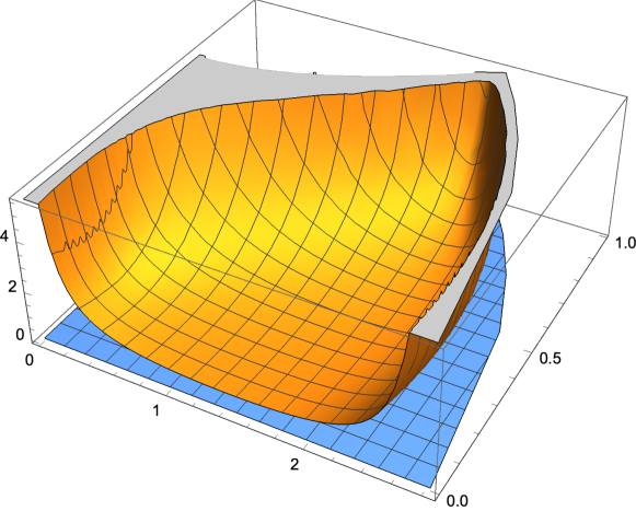
Figure 1. Graph of $c(g,\kappa,\mu)+c_{\kappa}(g,\kappa,\mu)\frac{K(\kappa)}{K^{\prime}(\kappa)}-2\mu c_{\mu}(g,\kappa,\mu)$ , for $\mu=1$

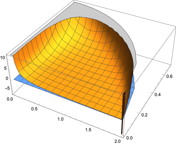
Figure 2. Graph of $c(g,\kappa,\mu)+c_{\kappa}(g,\kappa,\mu)\frac{K(\kappa)}{K^{\prime}(\kappa)}-2\mu c_{\mu}(g,\kappa,\mu)$ , for $\mu=-1$

Recall that both $Q,Q^{3}\subset Ker[\tilde{{\mathcal{L}}}_{+}]^{\perp}$ are bell-shaped, hence the function

$$\zeta(x):=Q(x)(Q^{2}(x)-Q^{2}(x_{0}))\perp Ker[\tilde{{\mathcal{L}}}_{+}].$$

satisfies $\zeta(x)>0,x\in(-x_{0},x_{0})$, $\zeta(x)<0,x\in(-1,-x_{0})\cup(x_{0},1)$. Thus, $\langle\zeta,\psi\rangle>0$, while $\zeta\perp Ker[\tilde{{\mathcal{L}}}_{+}]$. A contradiction is reached.

3.2.2. Proof of $n(\tilde{{\mathcal{L}}}_{+})=1$

In this section, we show the remaining claim in (3.12), namely that $\tilde{{\mathcal{L}}}_{+}$ has exactly one negative eigenvalue. Note that it suffices to prove $n({\mathcal{L}}_{+})=1$, as the operators ${\mathcal{L}}_{+},\tilde{{\mathcal{L}}}_{+}$ have the same Morse index.

To that end, note that Proposition 4 provides bell-shaped solutions for the profile equation (1.9), with the property $n({\mathcal{L}}_{+})=1$. We claim that at least one of the constrained minimizers in Proposition 4 is actually in the form of one of the solutions in Proposition 4. Going back to the full description of all possible bell-shaped solutions of (1.9), in Proposition 1, we see that the only other bell-shaped solutions are in the form $\varphi(0)=\varphi_{3},\varphi(-T)=\varphi(T)=0$ and $\varphi_{2}=\bar{\varphi}_{1},\varphi_{3}>0$.

Now, fix $c<0$. Also, select and fix sufficiently large half-period $T>\frac{1}{2|c|}\int_{0}^{1}\frac{dx}{\sqrt{x(1-x)}}dx$ and sufficiently small $L^{2}$ norm $\epsilon=\|v\|_{L^{2}}<<1$. Then, Proposition 4 guarantees a bell-shaped solution $V$, which in particular satisfies the Euler-Lagrange equation (2.5). We claim that $V$ is not of the form $V(0)=\varphi_{3},V(T)=V(-T)=0$. Once this is proven, we are done, since $V$ is then necessarily in the form of Proposition 5 and moreover, the corresponding linearized operator $L_{+}$ has exactly one negative eigenvalue.

Assume for a contradiction, that $V$ is of the form $V(0)=\varphi_{3},V(-T)=V(T)=0$. The difficulty with generating the solutions as constrained minimizers, as we just did is that we have no good control of the Lagrange multiplier $\zeta$, nor of the integration constant $a$. Instead, we have the parameters $T$ and $\|V\|_{L^{2}[-T,T]}^{2}$ to work with. Let us write the relations for the roots that we know. By the Viet’s formulas we have for $\varphi_{1},\varphi_{2}=\bar{\varphi}_{1}$,

$$\varphi_{1}+\varphi_{2}=4c-\varphi_{3}$$

Thus, we may compute

(3.20) $$T = \int_{0}^{T}d\varphi=\int_{0}^{\varphi_{3}}\frac{1}{\sqrt{\varphi(\varphi_{3}-\varphi)(\varphi-\varphi_{1})(\varphi-\bar{\varphi}_{1})}}d\varphi.$$

But since the roots $\varphi_{1},\varphi_{2}$ are complex-conjugate and $\varphi\geq 0$

$$(\varphi-\varphi_{1})(\varphi-\bar{\varphi}_{1})\geq(\varphi-\frac{\varphi_{1}+\bar{\varphi}_{1}}{2})^{2}=(\varphi-\frac{4c-\varphi_{3}}{2})^{2}\geq 4c^{2}.$$

It follows that

$$T\leq\frac{1}{2|c|}\int_{0}^{\varphi_{3}}\frac{1}{\sqrt{\varphi(\varphi_{3}-\varphi)}}d\varphi=\frac{1}{2c}\int_{0}^{1}\frac{1}{\sqrt{x(1-x)}}dx.$$

This is a contradiction with the choice of $T\geq\frac{1}{2c}\int_{0}^{1}\frac{1}{\sqrt{x(1-x)}}dx.$. It follows that $V$ is of the form of Proposition 5 and $n({\mathcal{L}}_{+})=1$. ∎

4. Spectral properties of ${\mathcal{L}}$

In this section, we tackle the spectral properties of the self-adjoint operator ${\mathcal{L}}$. This operator, due to its matrix structure is naturally harder to analyze than its scalar counterparts, ${\mathcal{L}}_{+},{\mathcal{L}}_{-}$. It turns out that it is possible to extract all the necessary spectral information, from the property

(4.1) $$\lambda_{0}({\mathcal{L}}_{+})<\lambda_{1}({\mathcal{L}}_{+})=0<\lambda_{2}({\mathcal{L}}_{+});\ \ Ker({\mathcal{L}}_{+})=span[\phi^{\prime}],$$

which was established in Proposition 6.

For $U=(u_{1},u_{2})$, where $u_{1}$ and $u_{2}$ are periodic functions with fundamental period $2T$, we have

(4.2) $$\langle{\mathcal{L}}U,U\rangle=\langle{\mathcal{L}}_{1}u_{1},u_{1}\rangle+\langle Mu_{2},u_{1}\rangle+\langle M^{*}u_{1},u_{2}\rangle+\langle{\mathcal{L}}_{2}u_{2},u_{2}\rangle$$

Let $u_{2}=\phi\tilde{u}_{2}$. After integrating by parts, we obtain

$$\langle{\mathcal{L}}_{2}u_{2},u_{2}\rangle = \langle\phi\partial_{y}\tilde{u}_{2},\phi\partial_{y}\tilde{u}_{2}\rangle$$

$$\langle Mu_{2},u_{1}\rangle+\langle M^{*}u_{1},u_{2}\rangle = \langle\phi^{3}\partial_{y}\tilde{u}_{2},u_{1}\rangle$$

Note that ${\mathcal{L}}_{1}={\mathcal{L}}_{+}+\frac{1}{4}\phi^{4}$. Hence,

(4.3) $$\langle{\mathcal{L}}U,U\rangle=\langle{\mathcal{L}}_{+}u_{1},u_{1}\rangle+\int_{-T}^{T}{\left[\frac{1}{2}\phi^{2}u_{1}+\phi(\phi^{-1}u_{2})_{y}\right]^{2}}dy.$$

This particular nice structure of the bilinear form $\langle{\mathcal{L}}U,U\rangle$, is not present, if one considers the linearized operator in the form (1.19). More specifically, there is an extra, sign-indefinite term in (4.3), namely $const.\langle\phi^{3}\partial_{y}\tilde{u}_{2},u_{1}\rangle$ which complicates the analysis of ${\mathcal{L}}$. This is why we needed to convert to the form (1.26). Concerning the kernel of ${\mathcal{L}}$, we have the following result.

4.1. Description of $Ker({\mathcal{L}})$

Proposition 7.

The operator ${\mathcal{L}}$ has at most one negative eigenvalue, i.e. $n({\mathcal{L}})\leq 1$. Next,
$dim(Ker({\mathcal{L}}))=2$. In fact,

$$Ker({\mathcal{L}})=span\{\Psi_{1},\Psi_{2}\},\Psi_{1}=\left(\begin{array}[]{c}0\\ \phi\end{array}\right),\Psi_{2}=\left(\begin{array}[]{c}\phi^{\prime}\\ -\frac{1}{4}\phi^{3}\end{array}\right).$$

Remark: We will show later that, as expected, $n({\mathcal{L}})=1$. Unfortunately, this cannot be done directly and requires some implicit analysis later on, see Section 5.2 below.

Proof.

Based on the formula (4.3) and (4.1), we see that if $u_{1}\perp\chi_{0}$ (where $\chi_{0}$ is the ground state for ${\mathcal{L}}_{+}$), then ${\mathcal{L}}|_{\{\chi_{0}\}^{\perp}}\geq 0$. Thus,

$$\inf\limits_{U\perp\left(\begin{array}[]{c}\chi_{0}\\ 0\end{array}\right)}\langle{\mathcal{L}}U,U\rangle\geq\inf\limits_{u_{1}\perp\chi_{0}}\langle{\mathcal{L}}_{+}u_{1},u_{1}\rangle\geq 0.$$

This implies that $n({\mathcal{L}})\leq 1$, as announced. We now discuss the structure of $Ker({\mathcal{L}})$.

It is convenient to split $L^{2}\times L^{2}=L^{2}_{even}\times L^{2}_{odd}\oplus L^{2}_{odd}\times L^{2}_{even}=:X_{e,o}\oplus X_{o,e}$ and since ${\mathcal{L}}$ acts invariantly on those subspaces, it suffices to determine $Ker({\mathcal{L}})$ on each.

Let us first show that $X_{o,e}=span[\Psi_{1},\Psi_{2}]$. Indeed, for $u_{1}\in L^{2}_{odd},u_{2}\in L^{2}_{even}$, we have that $u_{1}\perp\chi_{0}$, whence by the argument above, for $U=\left(\begin{array}[]{c}u_{1}\\ u_{2}\end{array}\right)\in X_{o,e}\cap Ker({\mathcal{L}})$,

$$0=\langle{\mathcal{L}}U,U\rangle\geq\langle{\mathcal{L}}_{+}u_{1},u_{1}\rangle\geq 0.$$

Recalling again that $u_{1}\perp\chi_{0}$, this implies that $u_{1}=0$ or $u_{1}=c\phi^{\prime}$. From (4.3), we have that the integral is zero as well, whence either $u_{2}=const.\phi$, when $u_{1}=0$ or else $u_{2}=-\frac{c}{4}\phi^{3}$, when $u_{1}=c\phi^{\prime}$. This completes the analysis on $X_{o,e}$.

Next, we show that $Ker({\mathcal{L}})\cap X_{e,o}=\{0\}$. This is a bit more complicated. Let $U=\left(\begin{array}[]{c}f\\ g\end{array}\right)\in X_{e,0}\cap Ker({\mathcal{L}})$. We set

(4.4) $$\left|\begin{array}[]{ll}{\mathcal{L}}_{1}f+Mg=0\\ \\ M^{*}f+{\mathcal{L}}_{2}g=0.\end{array}\right.$$

Not that $\langle M^{*}f,\phi\rangle=\langle f,M\phi\rangle=0$ and $Ker[{\mathcal{L}}_{2}]=Ker[{\mathcal{L}}_{-}]=span[\phi]$, so the second equation in (4.4) is solvable and in fact

(4.5) $$g=-{\mathcal{L}}_{2}^{-1}M^{*}f.$$

Next, we will be constructing Green function for the operator ${\mathcal{L}}_{2}^{-1}={\mathcal{L}}_{-}^{-1}$. We have ${\mathcal{L}}_{2}[\phi]=0$. The normalized function

$$\psi(x)=\phi(x)\int_{0}^{x}{\frac{1}{\phi^{2}(s)}}ds,\;\;\left|\begin{array}[]{cc}\phi&\psi\\ \phi^{\prime}&\psi^{\prime}\end{array}\right|=1$$

also solves ${\mathcal{L}}_{2}\psi=0$. The Green function, for an even function $f$ is represented by

$${\mathcal{L}}_{2}^{-1}M^{*}f(x)=\phi(x)\int_{0}^{x}{\psi(s)M^{*}f(s)}ds-\psi(x)\int_{0}^{x}{\phi(s)M^{*}f(s)}ds+C_{M^{*}f}\psi(x),$$

where $C_{M^{*}f}$ is a constant to be selected, so that ${\mathcal{L}}_{2}^{-1}f$ is periodic with same period as $\phi$. Integrating by parts yields

(4.6) $$\int_{0}^{x}\phi(s)M^{*}f(s)ds=-\frac{1}{2}\phi^{3}f+\frac{1}{2}\phi^{3}(0)f(0)$$

and

(4.7) $$\int_{0}^{x}{\psi(s)M^{*}f(s)}ds=-\frac{1}{2}\phi^{2}\psi f+\frac{1}{2}\int_{0}^{x}{\phi f}.$$

Also,

$$C_{M^{*}f} = -\frac{\phi(T)}{\psi(T)}\int_{0}^{T}{\psi M^{*}f}+\int_{0}^{T}{\phi M^{*}f}=-\frac{1}{2}\frac{1}{\int_{0}^{T}{\frac{1}{\phi^{2}}}dx}\int_{0}^{T}{\phi f}+\frac{1}{2}\phi^{3}(0)f(0)$$

$$= -\frac{d_{f}}{2d_{1}}+\frac{1}{2}\phi^{3}(0)f(0).$$

where

$$d_{1}=\frac{1}{\int_{0}^{T}{\frac{1}{\phi^{2}}}dx},\;\;d_{f}=\int_{0}^{T}\phi f.$$

All in all,

(4.8) $$g=\frac{d_{f}}{2d_{1}}\psi-\frac{\phi}{2}\int_{0}^{x}\phi f$$

Clearly, the formula for $g$ cannot be complete, without finding $f$, so we take this on now. Plugging (4.5) in the first equation of (4.4) results in

(4.9) $${\mathcal{L}}_{1}f-M{\mathcal{L}}_{2}^{-1}M^{*}f=0$$

After some algebraic manipulations, we obtain

$$M{\mathcal{L}}_{2}^{-1}M^{*}f = \frac{1}{4}\phi^{4}f-\frac{1}{4}\phi^{3}(0)f(0)\phi(x)+\frac{1}{2}C_{M^{*}f}\phi(x)$$

$$= \ \frac{\phi^{4}}{4}f-\frac{d_{1}d_{f}}{4}\phi.$$

Finally, the left-hand side of (4.9) is now in the form

$${\mathcal{L}}_{1}f-M{\mathcal{L}}_{2}^{-1}M^{*}f={\mathcal{L}}_{+}f+\frac{1}{4}d_{1}d_{f}\phi,$$

so, the equation to be solved is ${\mathcal{L}}_{+}f=-\frac{1}{4}d_{1}d_{f}\phi$. This equation has a solution, since $Ker({\mathcal{L}}_{+})=span[\phi^{\prime}]$. We obtain,

(4.10) $$f=-\frac{d_{1}d_{f}}{4}{\mathcal{L}}_{+}^{-1}[\phi].$$

This still does not mean that we have found an element in $Ker({\mathcal{L}})\cap X_{e,o}$, it simply means that if there is one, it must be in the form (4.10). There is still a consistency condition to be satisfied, namely about $d_{f}$. We take dot product with $\phi$. We obtain $2d_{f}=\langle f,\phi\rangle=-\frac{d_{1}d_{f}}{4}\langle{\mathcal{L}}_{+}^{-1}\phi,\phi\rangle,$ a relation that must be satisfied, in order to have a non-trivial element in $Ker({\mathcal{L}})\cap X_{e,o}$. This solvability condition amounts to

(4.11) $$d_{f}(8+d_{1}\langle{\mathcal{L}}_{+}^{-1}\phi,\phi\rangle)=0.$$

Clearly, if $d_{f}=0$, $f$ is trivial and this is not a new element of $Ker({\mathcal{L}})$. So, it remains that
$8+d_{1}\langle{\mathcal{L}}_{+}^{-1}\phi,\phi\rangle=0$. Equivalently, it must be that $4\int_{-T}^{T}\frac{1}{\phi^{2}}+\langle{\mathcal{L}}_{+}^{-1}\phi,\phi\rangle=0$. We however need this quantity later on, so we have computed it: see (5.1) for $\langle{\mathcal{L}}_{+}^{-1}\phi,\phi\rangle$ as well as the formula

$$\int_{-T}^{T}\frac{1}{\phi^{2}}=2g\int_{-K(\kappa)}^{K(\kappa)}\frac{1}{\varphi(2g\xi)}d\xi=\frac{4g}{\varphi_{1}\varphi_{3}}\left(\varphi_{3}K(\kappa)+(\varphi_{1}-\varphi_{3})\Pi\left[\frac{\varphi_{1}(\varphi_{3}-\varphi_{2})}{\varphi_{3}(\varphi_{1}-\varphi_{2})},\kappa\right]\right),$$

which we have done symbolically in Mathematica. As a result, we can display the following pictures, Figure 3 and Figure 4, which show that $4\int_{-T}^{T}\frac{1}{\phi^{2}}+\langle{\mathcal{L}}_{+}^{-1}\phi,\phi\rangle>0$,

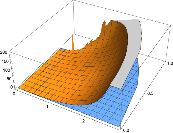
Figure 3. Graph of $4\int_{-T}^{T}\frac{1}{\phi^{2}}+\langle{\mathcal{L}}_{+}^{-1}\phi,\phi\rangle$ , for $\mu=1$

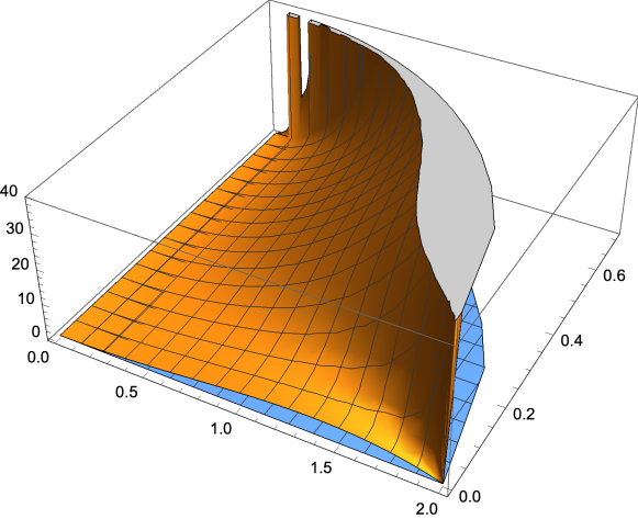
Figure 4. Graph of $4\int_{-T}^{T}\frac{1}{\phi^{2}}+\langle{\mathcal{L}}_{+}^{-1}\phi,\phi\rangle$ , for $\mu=-1$

This finishes the verification that $Ker({\mathcal{L}})\cap X_{e,o}=\{0\}$. ∎

4.2. Preliminary calculations for the matrix $D$

According to the setup described in (2.2), we setup the matrix $D$ as follows

$$D=\left(\begin{array}[]{cc}\langle{\mathcal{L}}^{-1}{\mathcal{J}}\Psi_{1},{\mathcal{J}}\Psi_{1}\rangle&\langle{\mathcal{L}}^{-1}{\mathcal{J}}\Psi_{1},{\mathcal{J}}\Psi_{2}\rangle\\ \langle{\mathcal{L}}^{-1}{\mathcal{J}}\Psi_{2},{\mathcal{J}}\Psi_{1}\rangle&\langle{\mathcal{L}}^{-1}{\mathcal{J}}\Psi_{2},{\mathcal{J}}\Psi_{2}\rangle\end{array}\right),$$

where $\Psi_{1},\Psi_{2}$ span $Ker({\mathcal{L}})$, they are described in Proposition 7. More explicitly,

$$D_{11}=\langle{\mathcal{L}}^{-1}{\mathcal{J}}\Psi_{1},{\mathcal{J}}\Psi_{1}\rangle = \langle{\mathcal{L}}^{-1}\left(\begin{array}[]{c}\phi\\ 0\end{array}\right),\left(\begin{array}[]{c}\phi\\ 0\end{array}\right)\rangle,$$

$$D_{12}=D_{21}=\langle{\mathcal{L}}^{-1}{\mathcal{J}}\Psi_{1},{\mathcal{J}}\Psi_{2}\rangle = \langle{\mathcal{L}}^{-1}{\mathcal{J}}\Psi_{2},{\mathcal{J}}\Psi_{1}\rangle=\langle{\mathcal{L}}^{-1}\left(\begin{array}[]{c}\phi\\ 0\end{array}\right),\left(\begin{array}[]{c}\frac{\phi^{3}}{4}\\ \phi^{\prime}\end{array}\right)\rangle,$$

$$D_{22}=\langle{\mathcal{L}}^{-1}{\mathcal{J}}\Psi_{2},{\mathcal{J}}\Psi_{2}\rangle = \langle{\mathcal{L}}^{-1}\left(\begin{array}[]{c}\frac{\phi^{3}}{4},\\ \phi^{\prime}\end{array}\right),\left(\begin{array}[]{c}\frac{\phi^{3}}{4}\\ \phi^{\prime}\end{array}\right)\rangle,$$

where the normalization constant satisfies $k\int_{0}^{L}\phi^{2}=\frac{1}{4}\int_{0}^{L}\phi^{4}$. We observe that since

$$\left(\begin{array}[]{c}\phi\\ 0\end{array}\right),\left(\begin{array}[]{c}\frac{\phi^{3}}{4}\\ \phi^{\prime}\end{array}\right)\perp span[\Psi_{1},\Psi_{2}]=Ker[{\mathcal{L}}]$$

we have that ${\mathcal{J}}:Ker({\mathcal{L}})\to Ker({\mathcal{L}})^{\perp}$, so it is justified to take ${\mathcal{L}}^{-1}$ in the above formulas.

As one can imagine, these quantities are quite hard to compute in general, especially with the involvement of the matrix Schrödinger operator ${\mathcal{L}}$. In fact, we have the following proposition, which establishes a reduced sufficient condition for stability of the waves $\phi$.

Proposition 8.

Assume (4.1). If

$$D_{11}=\langle{\mathcal{L}}^{-1}\left(\begin{array}[]{c}\phi\\ 0\end{array}\right),\left(\begin{array}[]{c}\phi\\ 0\end{array}\right)\rangle<0,$$

then $n(D)=1$ and the corresponding wave $\phi$ is stable. In fact, we have the formula

(4.15) $$D_{11}=\frac{4\int_{-T}^{T}\frac{1}{\phi^{2}}}{4\int_{-T}^{T}\frac{1}{\phi^{2}}+\langle{\mathcal{L}}_{+}^{-1}[\phi],\phi\rangle}\langle{\mathcal{L}}_{+}^{-1}[\phi],\phi\rangle$$

Remark: Note that the quantity in the denominator is positive, as established in the course of the proof of Proposition 7, see also Figures 3 and 4, which graphically confirm this. Thus, for all parameter values

$$sgn(D_{11})=sgn(\langle{\mathcal{L}}_{+}^{-1}[\phi],\phi\rangle)$$

Proof.

First, if $\langle{\mathcal{L}}^{-1}\left(\begin{array}[]{c}\phi\\ 0\end{array}\right),\left(\begin{array}[]{c}\phi\\ 0\end{array}\right)\rangle<0$, it follows from the min-max principle that ${\mathcal{L}}^{-1}$ has a negative eigenvalue, which implies that ${\mathcal{L}}$ has one too, hence $n({\mathcal{L}})\geq 1$. Since, we have already established, in Proposition 7, that $n({\mathcal{L}})\leq 1$, it would follows that $n({\mathcal{L}})=1$. Furthermore, for the matrix $D\in M_{2,2}$, we have $D_{11}=\langle De_{1},e_{1}\rangle<0$ means that $D$ too has a negative eigenvalue. Thus, $n(D)\geq 1$. Since we already know that $n({\mathcal{L}})=1$, formula (1.7) implies that $n(D)\leq 1$, so $n(D)=1$ and hence, we have stability, from (2.3). Thus, $D_{11}<0$ is sufficient for stability.

We now take on the question for the actual computation of $D_{11}$. Despite being arguably the easiest entry in the matrix $D$ to calculate, it is not an easy task to actually compute it. Its analysis is related to the analysis of $Ker({\mathcal{L}})$ in Proposition 7. Let

(4.16) $${\mathcal{L}}\left(\begin{array}[]{ll}f\\ g\end{array}\right)=\left(\begin{array}[]{ll}\phi\\ 0\end{array}\right),$$

which as we have observed is solvable in $X_{e,o}$, due to the fact that $\left(\begin{array}[]{ll}\phi\\ 0\end{array}\right)\perp Ker[{\mathcal{L}}]$. We note that such a solution comes with the property $\left(\begin{array}[]{ll}f\\ g\end{array}\right)\in Ker({\mathcal{L}})^{\perp}$. So, (4.16) is equivalent to

(4.17) $$\left|\begin{array}[]{ll}{\mathcal{L}}_{1}f+Mg=\phi\\ \\ M^{*}f+{\mathcal{L}}_{2}g=0.\end{array}\right.$$

Proceeding as in the proof of Proposition 7,

(4.18) $${\mathcal{L}}_{1}f-M{\mathcal{L}}_{2}^{-1}M^{*}f=\phi.$$

resulting in

(4.19) $${\mathcal{L}}_{+}f+\frac{1}{4}d_{1}d_{f}\phi=\phi,$$

where

$$d_{1}=\frac{1}{\int_{0}^{T}{\frac{1}{\phi^{2}}}dx},\;\;d_{f}=\int_{0}^{T}\phi f.$$

We obtain,

(4.20) $$f=(1-\frac{d_{1}d_{f}}{4}){\mathcal{L}}_{+}^{-1}[\phi].$$

Next, we determine $d_{f}$. We simply take dot product of (4.20) with $\phi$. We obtain the equation

$$2d_{f}=(1-\frac{d_{1}d_{f}}{4})\langle{\mathcal{L}}_{+}^{-1}\phi,\phi\rangle.$$

Let us note that this equation must have solutions as (4.4) does have a solution. In particular,

(4.21) $$d_{f}=\frac{\langle{\mathcal{L}}_{+}^{-1}\phi,\phi\rangle}{2+\frac{d_{1}}{4}\langle{\mathcal{L}}_{+}^{-1}\phi,\phi\rangle},$$

Since by definition, $D_{11}=2d_{f}$, we arrive at the formula (4.15). ∎

It becomes clear that in order to check for the stability, we need to be able to calculate various quantities like $\langle{\mathcal{L}}_{+}^{-1}\phi,\phi\rangle$. We have already computed that, subject to rescaling, see (3.19).

5. Analysis of the spectral stability for the bell-shaped waves of DNLS

In this section, we use our preliminary calculations, which allow us to compute the various quantities involved in the matrix $D$.

5.1. Computing $\langle{\mathcal{L}}_{+}^{-1}\phi,\phi\rangle$

In the calculations for $D_{11}$, see (4.15), a major role is played by $\langle{\mathcal{L}}_{+}^{-1}\phi,\phi\rangle$. In order to compute that, we use the formula (3.19), which gives $\tilde{L}^{-1}Q$, in the rescaled framework of Section 3.2.

So, let us continue to use the setup introduced in Section 3.2 and more precisely in the equation (3.11). By taking dot product of (3.19) with $Q$, we obtain

$$\langle\tilde{{\mathcal{L}}}_{+}^{-1}Q,Q\rangle = 16T^{-2}\frac{\frac{c_{\mu}}{2}\langle Q,Q\rangle+c_{\mu}\frac{K(\kappa)}{K^{\prime}(\kappa)}\langle Q_{\kappa},Q\rangle-\left(c+c_{\kappa}\frac{K(\kappa)}{K^{\prime}(\kappa)}\right)\langle Q_{\mu},Q\rangle}{c+c_{\kappa}\frac{K(\kappa)}{K^{\prime}(\kappa)}-2\mu c_{\mu}},$$

where recall that the function $c=c(A,B,C)$ is given explicitly in (3.7), while the quantities $A,B,C$, all in terms of $g,\kappa,\mu$ are explicitly in (3.1), (3.2), (3.3).

We have, $\langle Q,Q\rangle=T^{-1}\|\phi\|^{2}$. Also, since $T=T(g,\kappa)$ is independent on $\mu$,

$$\langle Q_{\mu},Q\rangle=\int_{-1}^{1}Q_{\mu}(\xi)Q(\xi)d\xi=\frac{1}{2}\partial_{\mu}\int_{-1}^{1}Q^{2}(\xi)d\xi=\frac{1}{2}\partial_{\mu}T^{-1}\|\phi\|^{2}=\frac{T^{-1}}{2}\partial_{\mu}\|\phi\|^{2}$$

On the other hand,

$$\langle Q_{\kappa},Q\rangle=\int_{-1}^{1}Q_{\kappa}(\xi)Q(\xi)d\xi=\frac{1}{2}\partial_{\kappa}\int_{-1}^{1}Q^{2}(\xi)d\xi=\frac{1}{2}\partial_{\kappa}[T^{-1}\|\phi\|^{2}]=\frac{T^{-1}}{2}\partial_{\kappa}\|\phi\|^{2}-\frac{T^{-2}T_{\kappa}}{2}\|\phi\|^{2}.$$

Thus, we have reduced matters to computing the following formula

$$\langle\tilde{{\mathcal{L}}}_{+}^{-1}Q,Q\rangle = 16T^{-2}\frac{\frac{c_{\mu}}{2}T^{-1}\|\phi\|^{2}+c_{\mu}\frac{K(\kappa)}{K^{\prime}(\kappa)}(\frac{T^{-1}}{2}\partial_{\kappa}\|\phi\|^{2}-\frac{T^{-2}T_{\kappa}}{2}\|\phi\|^{2})-\left(c+c_{\kappa}\frac{K(\kappa)}{K^{\prime}(\kappa)}\right)\frac{T^{-1}}{2}\partial_{\mu}\|\phi\|^{2}}{c+c_{\kappa}\frac{K(\kappa)}{K^{\prime}(\kappa)}-2\mu c_{\mu}}$$

$$= 16T^{-3}\frac{\frac{c_{\mu}}{2}\|\phi\|^{2}+c_{\mu}\frac{K(\kappa)}{K^{\prime}(\kappa)}(\frac{1}{2}\partial_{\kappa}\|\phi\|^{2}-\frac{K^{\prime}(\kappa)}{2K(\kappa)}\|\phi\|^{2})-\left(c+c_{\kappa}\frac{K(\kappa)}{K^{\prime}(\kappa)}\right)\frac{1}{2}\partial_{\mu}\|\phi\|^{2}}{c+c_{\kappa}\frac{K(\kappa)}{K^{\prime}(\kappa)}-2\mu c_{\mu}}=$$

$$= 8T^{-3}\frac{c_{\mu}\frac{K(\kappa)}{K^{\prime}(\kappa)}\partial_{\kappa}\|\phi\|^{2}-\left(c+c_{\kappa}\frac{K(\kappa)}{K^{\prime}(\kappa)}\right)\partial_{\mu}\|\phi\|^{2}}{c+c_{\kappa}\frac{K(\kappa)}{K^{\prime}(\kappa)}-2\mu c_{\mu}}.$$

Since $\langle\tilde{{\mathcal{L}}}_{+}^{-1}Q,Q\rangle=T^{-3}\langle{\mathcal{L}}_{+}^{-1}\phi,\phi\rangle$, we arrive at the formula

(5.1) $$\langle{\mathcal{L}}_{+}^{-1}\phi,\phi\rangle=8\frac{c_{\mu}\frac{K(\kappa)}{K^{\prime}(\kappa)}\partial_{\kappa}\|\phi\|^{2}-\left(c+c_{\kappa}\frac{K(\kappa)}{K^{\prime}(\kappa)}\right)\partial_{\mu}\|\phi\|^{2}}{c+c_{\kappa}\frac{K(\kappa)}{K^{\prime}(\kappa)}-2\mu c_{\mu}}.$$

As we saw earlier, the denominator is never zero, per explicit calculations done earlier, see Figure 1 and Figure 2 for a particular slices at $\mu=1$, $\mu=-1$ respectively.

Thus, we need to evaluate $\|\phi\|_{L^{2}}^{2}$in terms of $g,\kappa,\mu$. Using Mathematica, we computed

$$\|\phi\|_{L^{2}}^{2} = 2g\int_{-K(\kappa)}^{K(\kappa)}\varphi(2g\xi)d\xi=4g\left(\varphi_{1}K(\kappa)+(\varphi_{3}-\varphi_{1})\Pi\left[\frac{\varphi_{3}-\varphi_{2}}{\varphi_{1}-\varphi_{2}},\kappa\right]\right),$$

where $\Pi$ is the elliptic $\Pi$ function.

With this formula in hand, we compute the quantities in (5.1) using Mathematica. The results can be seen in the slices of the graphs for $\langle{\mathcal{L}}_{+}^{-1}\phi,\phi\rangle$, in Figure 5, for $\mu=1$ and Figure 6 for $\mu=-1$. From these images (and this is the case for all values of $\mu$ that we have tried), the expression $\langle{\mathcal{L}}_{+}^{-1}\phi,\phi\rangle$ always changes sign over the domain. In particular, there is a always a region $\tilde{\Omega}$, where it takes negative values. It follows that $D_{11}$ vanishes on a curve in the domains, and it takes positive and negative values as well.

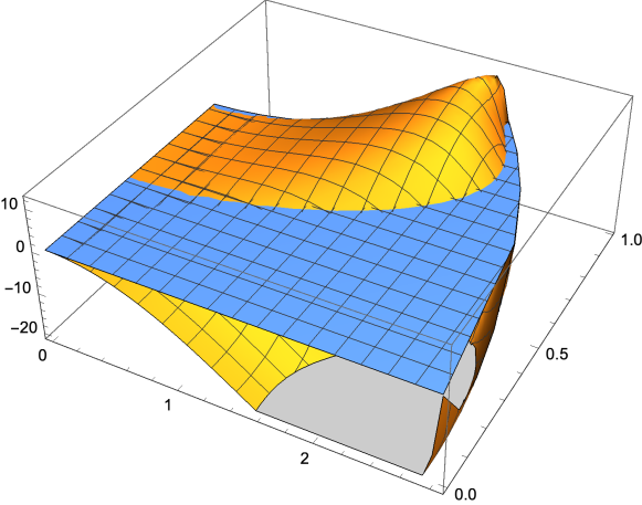
Figure 5. Graph of $\langle{\mathcal{L}}_{+}^{-1}\phi,\phi\rangle$ , for $\mu=1$

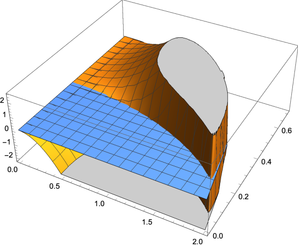
Figure 6. Graph of $\langle{\mathcal{L}}_{+}^{-1}\phi,\phi\rangle$ , for $\mu=-1$

5.2. $n({\mathcal{L}})=1$ and the waves with $\langle{\mathcal{L}}_{+}^{-1}\phi,\phi\rangle<0$ are spectrally stable

In this section, we finally confirm that $n({\mathcal{L}})=1$. This is achieved by piecing together several conclusions established in the previous sections.

We have already seen that $n({\mathcal{L}})\leq 1$ in Proposition 7. We have argued in the previous section that that the quantity $\langle{\mathcal{L}}_{+}^{-1}\phi,\phi\rangle$ is always negative, somewhere in the parameter domain, see also Figures 5, 6. Thus, according to (4.15), $sgn(D_{11})=sgn(\langle{\mathcal{L}}_{+}^{-1}\phi,\phi\rangle)=-1$ on a portion of the domain. Thus, it follows that $n(D)\geq 1$, somewhere in the parameter domain. On the other hand, from the instability index theory, see (2.3), we always have the inequality $n({\mathcal{L}})\geq n(D)$, so $n({\mathcal{L}})\geq 1$ somewhere on the parameter domain. We claim that $n({\mathcal{L}})=1$ for all values in the parameter domain. Indeed, if $n({\mathcal{L}})=1$ somewhere on it, a potential transition to $n({\mathcal{L}})=0$, due to the continuous dependence on the parameters, happens only if the negative eigenvalue crosses the zero en route to becoming a positive one. This would require, at least for some value of the parameters to have three vectors in $Ker({\mathcal{L}})$. According to Proposition 7, this is not the case. Thus, $n({\mathcal{L}})=1$ for all parameters described in Proposition 5. Hence, as discussed after (2.3), the stability of the waves is equivalent to $n(D)=1$ or equivalently, $det(D)<0$.

In particular, since $n(D)\geq 1$, whenever $\langle{\mathcal{L}}_{+}^{-1}\phi,\phi\rangle<0$, we have that $k_{Ham}=n({\mathcal{L}})-n(D)=0$, hence spectral stability holds for these values.

5.3. $D_{12}$ and $D_{11}$ do not vanish simultaneously: conclusion of the proof

We need to establish that

$$D_{12}=\langle f,\frac{\phi^{3}}{4}\rangle+\langle g,\phi^{\prime}\rangle,$$

with $f,g$ as introduced in (4.16) does not vanish simultaneously with $D_{11}$. Let us consider the expression for $D_{12}$, exactly on the set where $D_{11}=0$. Clearly $D_{11}=0$ exactly when $\langle{\mathcal{L}}_{+}^{-1}\phi,\phi\rangle=0$ and since $f=const.{\mathcal{L}}_{+}^{-1}\phi$, precisely when $\langle f,\phi\rangle=0$. Thus, on this set, we can check that $g=-\frac{\phi}{2}\int_{0}^{x}f\phi$. But, on the set $\{D_{11}=0\}$, an integration by parts shows

$$D_{12}=\langle f,\frac{\phi^{3}}{4}\rangle+\langle g,\phi^{\prime}\rangle=\frac{1}{2}\langle f,\phi^{3}\rangle=const.\langle{\mathcal{L}}_{+}^{-1}\phi,\phi^{3}\rangle.$$

Thus, it suffices to check $\langle{\mathcal{L}}_{+}^{-1}\phi,\phi\rangle,\langle{\mathcal{L}}_{+}^{-1}\phi,\phi^{3}\rangle$ do not vanish simultaneously. To this end, recall that $n({\mathcal{L}}_{+})=1,Ker[{\mathcal{L}}_{+})=span[\phi^{\prime}]$, and denote its positive ground state of ${\mathcal{L}}_{+}$ by $\Psi_{0}$. Clearly, $\langle\phi,\Psi_{0}\rangle>0,\langle\phi^{3},\Psi_{0}\rangle>0$. This, there is a scalar $c_{0}>0$, so that $\langle\phi-c_{0}\phi^{3},\Psi_{0}\rangle=0$. It follows that

(5.2) $$\langle{\mathcal{L}}_{+}^{-1}\phi,\phi\rangle-c_{0}\langle{\mathcal{L}}_{+}^{-1}\phi,\phi^{3}\rangle=\langle{\mathcal{L}}_{+}^{-1}\phi,\phi-c_{0}\phi^{3}\rangle=\langle{\mathcal{L}}_{+}^{-1}P_{\{\Psi_{0},\phi^{\prime}\}^{\perp}}\phi,P_{\{\Psi_{0},\phi^{\prime}\}^{\perp}}(\phi-c_{0}\phi^{3})\rangle>0,$$

because $P_{\{\Psi_{0},\phi^{\prime}\}^{\perp}}$ restricts to the positive subspace of ${\mathcal{L}}_{+}^{-1}$. This last inequality (5.2) shows that $\langle{\mathcal{L}}_{+}^{-1}\phi,\phi\rangle,\langle{\mathcal{L}}_{+}^{-1}\phi,\phi^{3}\rangle$ cannot not vanish simultaneously.

6. Stability analysis for the quintic NLS waves

The spectral problem (1.38) is easy to analyze, with the tools that we have prepared so far. Indeed, by Proposition (6), we have seen that $n({\mathcal{L}}_{+})=1$, while $n({\mathcal{L}}_{-})=0$. In addition, $Ker({\mathcal{L}}_{+})=span[\phi^{\prime}]$, while $Ker({\mathcal{L}}_{-})=span[\phi]$. Applying index counting theory (and more specifically (2.3)), we see that the matrix $D$ is one dimensional, namely $D_{11}=\langle{\mathcal{L}}_{+}^{-1}\phi,\phi\rangle$. In addition, $k_{Ham}=0$ (and hence the waves are stable) exactly when $\langle{\mathcal{L}}_{+}^{-1}\phi,\phi\rangle<0$ and unstable, if
$\langle{\mathcal{L}}_{+}^{-1}\phi,\phi\rangle>0$, with a change of instability (and an additional element in the generalized kernel in the Hamiltonian linearized operator (1.38) for $\langle{\mathcal{L}}_{+}^{-1}\phi,\phi\rangle=0$. Thus, we need to find $\langle{\mathcal{L}}_{+}^{-1}\phi,\phi\rangle$, for this new restricted set of parameters. We set on to describe the waves in the style of Proposition 5.

Proposition 9.

Let

(6.1) $$0<g<\infty\ \ \&\ \ \kappa\in(0,1)\ \ \&\ \ \mu=\frac{4\sqrt{1-k^{2}+k^{4}}}{g^{2}}$$

Let the roots $\varphi_{1},\varphi_{2},\varphi_{3}$ are as described in (3.6). Then, the two family of waves (corresponding to $\pm$ values of $\mu$) described in (1.36) are parametrized by $g,\kappa$ are all non-vanishing bell-shaped waves of the quintic NLS.

Proof.

Recall that the waves (1.36) correspond to those of (1.12), with the condition $c=0$. Solving in the formula for $c$ from (3.7), $c=0$, we end up with the relation $AB+BC-AC=0$, which is solved in terms of $\mu$ to exactly $\mu=\frac{4\sqrt{1-k^{2}+k^{4}}}{g^{2}}$. Finally, note that the constraint for $\mu$ ensures that the inequalities required in (3.9), namely $g<\sqrt{\frac{8}{\mu}}.$ is satisfied. This completes the proof of Proposition 9. ∎

Our next task is to determine the sign of the quantity $\langle{\mathcal{L}}_{+}^{-1}\phi,\phi\rangle$, on the set of parameters outlined in the constraint (6.1). We have plotted the graph of the relevant graph in Figure 7. It shows almost perfect stability result for $0<\kappa<0.54$ and instability for $\kappa\in(0.54,1)$.

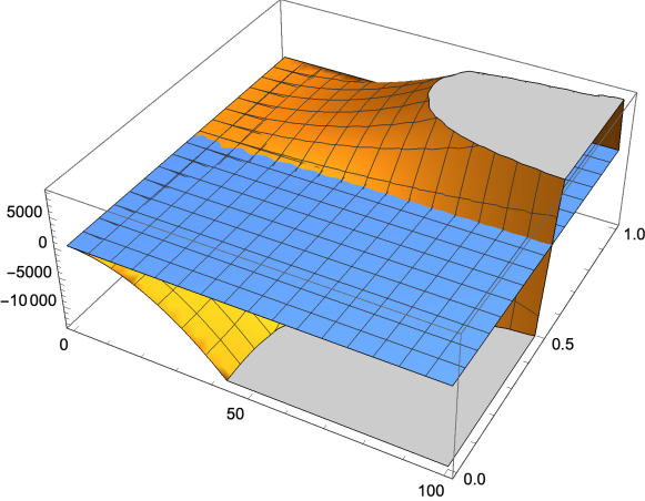
Figure 7. Graph of $\langle{\mathcal{L}}_{+}^{-1}\phi,\phi\rangle$ for quintic NLS waves

References

- [1] H. Bahouri, G. Perelman, Global well-posedness for the derivative nonlinear Schrödinger equation, preprint.
- [2] T. B. Benjamin, The stability of solitary waves, R. Soc. Lond. Proc. Ser. A Math. Phys. Eng. Sci., 328, (1972), p. 153–183.
- [3] H.A. Biagioni, F. Linares, Ill-posedness for the derivative Schrödinger and generalized Benjamin-Ono equations, Trans. Amer. Math. Soc. 353, (2001), no. 9, p. 3649–3659.
- [4] J. Chen, D. Pelinovsky, J. Upsal, Modulational instability of periodic standing waves in the derivative NLS equation, preprint available at https://arxiv.org/pdf/2009.05425.pdf.
- [5] J. Chen, D. Pelinovsky, Periodic travelling waves of the modified KdV equation and rogue waves on the periodic background, J. Nonlinear Sci. 29, (2019), no. 6, p. 2797–2843.
- [6] J. Chen, R. Zhang, The complex Hamiltonian systems and quasi-periodic solutions in the derivative nonlinear Schrödinger equations, Stud. Appl. Math., 145, (2020), no. 2, p. 153–178.
- [7] M. Colin, Mathieu; M. Ohta, Stability of solitary waves for derivative nonlinear Schrödinger equation, Ann. Inst. H. Poincaré Anal. Non Linéaire,. 23, (2006), no. 5, p. 753–764.
- [8] B. L. Guo, Y. Wu, Orbital stability of solitary waves for the nonlinear derivative Schrd̈inger equation, J. Differential Equations, 123, (1995), no. 1, p. 35–55.
- [9] R. Jenkins, J. Liu, P. Perry, C. Sulem, Soliton resolution for the derivative nonlinear Schrödinger equation, Comm. Math. Phys., 363, (2018), no. 3, p. 1003–1049.
- [10] N. Hayashi, T. Ozawa, On the derivative nonlinear Schrödinger equation, Phys. D, 55, (1992), no. 1-2, p. 14–36.
- [11] N. Hayashi, T. Ozawa, Finite energy solutions of nonlinear Schrödinger equations of derivative type, SIAM J. Math. Anal., 25, (1994), no. 6, p. 1488–1503.
- [12] S. Herr, On the Cauchy problem for the derivative nonlinear Schrödinger equation with periodic boundary condition. Int. Math. Res. Not. 2006, Art. ID 96763, 33 pp.
- [13] T. M. Kapitula, P. G. Kevrekidis, B. Sandstede, Counting eigenvalues via Krein signature in infinite-dimensional Hamitonial systems, Physica D, 3-4, (2004), p. 263–282.
- [14] T. Kapitula,P. G. Kevrekidis, B. Sandstede, Addendum: ”Counting eigenvalues via the Krein signature in infinite-dimensional Hamiltonian systems” [Phys. D 195 (2004), no. 3-4, 263–282] Phys. D 201 (2005), no. 1-2, 199–201.
- [15] T. Kapitula, K. Promislow, Spectral and dynamical stability of nonlinear waves. Applied Mathematical Sciences, 185, Springer, New York, 2013.
- [16] Z. Lin, C. Zeng, Instability, index theorem, and exponential trichotomy for Linear Hamiltonian PDEs, available at https://arxiv.org/abs/1703.04016, to appear as Mem. Amer. Math. Soc.
- [17] J. Liu, P.A. Perry, C. Sulem, Global existence for the derivative nonlinear Schrödinger equation by the method of inverse scattering, Comm. PDE, 41, (11) (2016) p. 1692–1760.
- [18] J. Liu, P.A. Perry, C. Sulem, Long-time behavior of solutions to the derivative nonlinear Schrödinger equation for soliton-free initial data, Ann. Inst. Henri Poincaré, Anal. Non Linéaire, 35(1), (2018), p. 217–265.
- [19] X. Liu, G. Simpson, C. Sulem, Stability of solitary waves for a generalized derivative nonlinear Schrödinger equation, J. Nonlinear Sci. 23 (2013), no. 4, p. 557–583.
- [20] W. Mio, T. Ogino, K. Minami, S. Takeda, Modified nonlinear Schrödinger equation for Alfven waves propagating along the magnetic field in cold plasmas, J. Phys. Soc. Jpn., 41, (1976), p. 265–271.
- [21] C. Miao, X. Tang, G. Xu, Stability of the traveling waves for the derivative Schrödinger equation in the energy space, Calc. Var. Partial Differential Equations, 56, (2017), no. 2, Paper No. 45, 48 pp.
- [22] E. Mjolhus, On the modulational instability of hydromagnetic waves parallel to the magnetic field, J. Plasma Phys. 16, (1976) p. 321–334.
- [23] T. Ozawa, On the nonlinear Schrödinger equations of derivative type, Indiana Univ. Math. J., 45, (1996), p. 137–163.
- [24] D. Pelinovsky, Inertia law for spectral stability of solitary waves in coupled nonlinear Schrödinger equations. Proc. R. Soc. Lond. Ser. A Math. Phys. Eng. Sci. 461 (2005) , no. 2055, p. 783–812.
- [25] D. Pelinovsky, A. Saalmann, Y. Shimabukuro, The derivative NLS equation: global existence with solitons, Dyn. Partial Differ. Equ., 14, (2017), 3, p. 271–294.
- [26] D. Pelinovsky, Y. Shimabukuro, Existence of global solutions to the derivative NLS equation with the inverse scattering transform method, Int. Math. Res. Not. 2018, no. 18, p. 5663–5728.
- [27] H. Takaoka, Well-posedness for the one dimensional Schrödinger equation with the derivative nonlinearity, Adv. Differ. Equ. 4, (1999), p. 561–580.
- [28] H. Takaoka. Global well-posedness for Schrödinger equations with derivative in a nonlinear term and data in low-order Sobolev spaces. Electron. J. Diff. Eq, 42, (2001), 23 pp.
- [29] J. Upsal, B. Deconinck, Real Lax spectrum implies spectral stability, Stud. Appl. Math., 145, (2020), no. 4, p. 765–790.