Diffraction of diatomic molecular beams: a model with applications to Talbot-Lau interferometry

Abstract

In this article we formulate and solve the problem of molecular beam diffraction when each molecule consists of two interacting bodies. Then, using our results, we present the diffraction patterns for various molecular sizes employing the harmonic oscillator as interaction model between the two atoms. Lastly, we analyze the corrections produced by the internal structure of the molecule in applications that include beam focusing and Talbot carpets.

I Introduction

The microscopic effects of Quantum Mechanics have been studied for more than a century by means of diverse experiments. Mesoscopic effects, on the other hand, are more rare and their realizations are more recent blochManybodyPhysicsUltracold2008 . For instance, manifestations of quantum physics in macroscopic objects are hard to attain due to decoherence campbellAtomicEnvoyEnables2017a . Interestingly, in recent years brezgerConceptsNearfieldInterferometers2003 ; truppeBufferGasBeam2018 ; dorrePhotofragmentationBeamSplitters2014 ; chapmanOpticsInterferometryNa1995 ; brezgerMatterWaveInterferometerLarge2002 ; haslingerUniversalMatterwaveInterferometer2013 ; hornbergerColloquiumQuantumInterference2012 it has been found that matter waves made of large organic molecules can exhibit interference phenomena that manifest in diffraction patterns. Accordingly, they are susceptible of wave-like treatments caseDiffractiveMechanismFocusing2012 as dictated by the Schrödinger equation, and they can be manipulated for interferometry experiments gerlichKapitzaDiracTalbot2007a that are related, among other subjects, to metrology (nawrockiIntroductionQuantumMetrology2019, , p. 223-224).

In this work, we are interested in the diffraction patterns produced by molecular beams passing through slits or periodic electromagnetic fields. This setting has provided clear evidence on the fact that composites as massive as 2000 molecular units undergo interference phenomena summyMolecularInterferometryMakes2014a . Despite the great body of work on this area, such processes have not been described analytically in full extension. A treatment of the full wave equation that includes the propagation of all the constituents in a molecule, together with their analytical solutions, is still lacking.

Notable attempts have been made on the scattering analysis of classical and quantum-mechanical objects with internal structure or finite extension shoreScatteringParticleInternal2015 , domotorScatteringParticleInternal2015 . In those precedents, important model simplifications such as the restriction of the center-of-mass motion to a line and the constraint of internal molecular motion to classical rigidity led to concrete theoretical results on the existence of resonances at a slit acting as a scatterer. However, this also has brought limitations regarding the predictive power of the model, and it has made evident the need for more realistic treatments. For example, we note that transmission and reflection coefficients are based only on far field properties, and not on the full diffraction pattern. More recently, a classical attempt to include more degrees of freedom in the center of mass motion domotorScatteringClassicalRotor2019 led to the conclusion that signatures of chaos could be found in the dynamics. While this seems to be a downside, we are sure that quantum dynamics of a few molecular levels are not really affected by classical chaos and a comprehensive description of the scattering process should be possible. This also makes clear that, for wave-like extended objects, the models in shoreScatteringParticleInternal2015 are too simple to describe the associated diffraction fields in all regions.

Here we present an original framework that uses the molecular wave function in order to provide explicit results of probability densities and diffraction patterns. Previously, in condadoDiffractionParticlesFree2018 , matter wave diffraction was analyzed with the aim of studying the effect of gravity in freely falling point-like particles. The contribution of this work is to provide the corrections when a harmonic molecule is considered. As an example, we present a Talbot carpet in fig. 1 corrected by the motion of internal structure, which is modelled as a harmonic oscillator between two atoms. The treatment leading to this depiction will be explained in further sections.

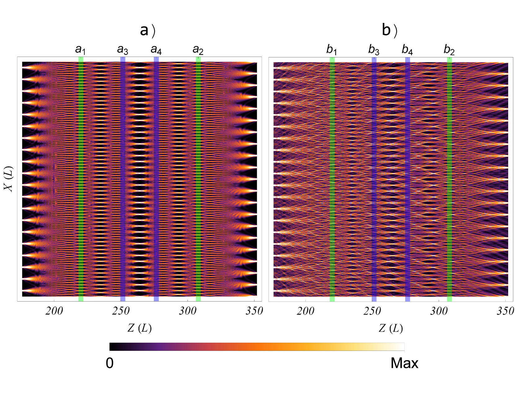
Figure 1: Diffraction patterns known as Talbot carpets, produced by eq. (LABEL:Talbot_marginal_probability_density) for a diffractive grating. Square pulses emerge from each slit (compare with periodic conditions implemented in other realizations caseRealizationOpticalCarpets2009 ). The period of the grating is $8L$ with $L$ the size of a slit. In a) we see a carpet produced by a point-like particle, shown in a window ranging from the first secondary revival to the first primary revival. The wavelength-dependent energy was introduced by $\lambda/L=0.363$. In b) we see the carpet produced by a diatomic molecule, again seen from the first secondary revival to the first primary revival and $\lambda/L=0.363$. The molecular radius $a$ in terms of the oscillator parameters $\sqrt{\hbar/m\omega}$ is chosen as $a/L=0.335$. Important differences can be noted: a focusing between $a_{3}$ and $a_{4}$ also occurs between $b_{3}$ and $b_{4}$, but the pattern is asymmetric in the second case.

Structure of the paper: In section II we define our boundary value problem, requiring the presence of absorptive screens and finding thereby the general solution of the Schrödinger equation under such conditions. In section III we use the harmonic oscillator as a model for the interaction between the atoms in the molecule and apply our formulas to specific cases and parameters. We present plots of the resulting patterns in the far, intermediate and near field regions, as well as comparisons between them. In section IV, the effect of the internal structure on Talbot carpets is obtained. Finally, in V we make some observations regarding our results.

II Definition of the molecular diffraction problem and its solution

II.1 General considerations

The system we want to study consists of two interacting quantum particles, bound by a central potential. After being freely propagated in the center of mass, the atoms have contact with an absorptive screen and a diffraction pattern appears on the opposite side. The existence of two particles requires six degrees of freedom, whose variables satisfy the following commutation relations:

$$\left[x^{i}_{l},x^{j}_{m}\right] = 0=\left[p^{i}_{l},p^{j}_{m}\right],$$

$$\left[x^{i}_{l},p^{j}_{m}\right] = i\hbar\delta_{ij}\delta_{lm},$$ (1)

where the subscripts account for each particle and the superscripts for their components. For problems with translational symmetry (e.g. infinite slits) we may opt for a model reduced to four-dimensional space, i.e. $i,j=1,2$ and coordinates $\vec{x_{1}}=(x_{1},z_{1}),\vec{x_{2}}=(x_{2},z_{2})$. We work with the following Hamiltonian:

$$\begin{split}\hat{H}&=\frac{\vec{p_{1}}^{2}}{2m_{1}}+\frac{\vec{p_{2}}^{2}}{2m_{2}}+V(|\vec{x_{2}}-\vec{x_{1}}|)\\ &=-\frac{\hbar^{2}}{2m_{1}}\nabla^{2}_{1}-\frac{\hbar^{2}}{2m_{2}}\nabla^{2}_{2}+V(|\vec{x_{2}}-\vec{x_{1}}|),\end{split}$$ (2)

where $m_{1}$ and $m_{2}$ are the inertial masses of the bodies. As it is usual, we separate the problem in relative and center-of-mass coordinates:

$$\begin{split}\vec{x}&=\vec{x_{2}}-\vec{x_{1}}\equiv x\hat{x}+z\hat{z}\\ \vec{X}&=\frac{m_{1}\vec{x_{1}}+m_{2}\vec{x_{2}}}{M}\equiv X\hat{x}+Z\hat{z},\end{split}$$ (3)

where $M=m_{1}+m_{2}$ is the total mass. With this change, we may work with the following operator

$$\begin{split}\hat{H}&=-\frac{\hbar^{2}}{2M}\nabla^{2}_{X}-\frac{\hbar^{2}}{2\mu}\nabla^{2}_{x}+V(r),\end{split}$$ (4)

where

$$\begin{split}\mu=\frac{m_{1}m_{2}}{m_{1}+m_{2}},\quad r=|\vec{x_{2}}-\vec{x_{1}}|,\quad\theta=\arctan\left(\frac{x_{2}-x_{1}}{z_{2}-z_{1}}\right).\end{split}$$ (5)

As can be noted, the stationary wave equation associated with (4) requires a mutivariable Green’s function that must be obtained from scratch. Also, a pattern obtained at a distance $Z$ from a plate should represent the probability density in the event that the center of mass of the molecule hits the detection screen. This, in turn, demands that only the two variables $X,Z$ must survive after the corresponding propagation is calculated; we shall address this in the next section. See diagrams in fig. 2 and 3.

II.2 Schrödinger equation of the molecular diffraction problem

The stationary Schrödinger equation at hand is

$$\left\{-\frac{\hbar^{2}}{2M}\nabla^{2}_{X}-\frac{\hbar^{2}}{2\mu}\nabla^{2}_{x}+V(|\vec{x_{2}}-\vec{x_{1}}|)\right\}\psi=E\psi,$$ (6)

and by separating it, we obtain:

$$\begin{gathered}\psi=\Psi_{X}\chi_{x}\\ -\frac{\hbar^{2}}{2M}\nabla^{2}_{X}\Psi_{X}=E_{X}\Psi_{X}\\ -\frac{\hbar^{2}}{2\mu}\nabla^{2}_{x}\chi_{x}+V(r)\chi_{x}=E_{x}\chi_{x},\end{gathered}$$ (7)

where the separation constants $E_{X}$ and $E_{x}$ satisfy

$$E_{X}+E_{x}=E.$$ (8)

Although (6) and (7) are separable solutions, a fixed energy $E$ has many possible associated products of waves $\Psi_{X}\chi_{x}$ due to degeneracy. Therefore, a general solution of (6) is a superposition of such products in relative and center-of-mass coordinates. The wave functions are further constrained by the boundary condition at the slit, i.e. the initial condition at $Z=0$ if $Z$ is regarded as a pseudo-time. It should be mentioned that trivial expressions given by factorizable solutions in all spatial regions have total lack of value; we anticipate thus that gratings have the effect of mixing quantum numbers after diffraction takes place.

II.3 General solutions, explicit propagators and marginal probability

The explicit factors in (7) are

$$\begin{gathered}\Psi_{X}(\vec{X})=\frac{1}{2\pi}e^{i\vec{K}\cdot\vec{X}}=\frac{1}{2\pi}e^{i(K_{X}X+K_{Z}Z)}\\ \chi_{x}(\vec{x})=\phi_{n\,l}(\vec{x})=\phi_{n\,l}(r,\theta)=R_{n\,l}(r)e^{il\theta}.\end{gathered}$$ (9)

Here, the functions $\phi_{n\,l}(\vec{x})$ can be expressed also in polar coordinates $r,\theta$. They must satisfy the following orthogonality relations:

$$\int_{0}^{2\pi}\int_{0}^{\infty}rdrd\theta\phi_{n\,l}(r,\theta)\phi^{*}_{n^{\prime}\,l^{\prime}}(r,\theta)=\delta_{n\,n^{\prime}}\delta_{l\,l^{\prime}}.$$ (10)

The subscripts $n,l$ come from internal energy quantization in two dimensions, e.g. in a central binding potential $n,l$ represent the radial and angular momentum numbers, respectively. The internal energy of the molecule is directly related to the separation constant in (8): $\epsilon_{nl}=E_{x}$.

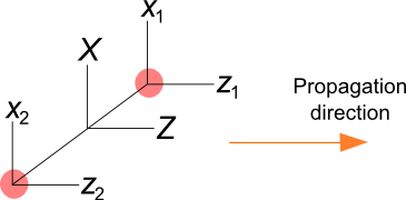
Figure 2: Internal and center of mass Cartesian coordinates.

From (9), we can see that the dispersion relation of Schrödinger waves, understood as $\omega_{k}=E/\hbar$, has the form

$$\frac{\hbar^{2}K_{X}^{2}}{2M}+\frac{\hbar^{2}K_{Z}^{2}}{2M}+\epsilon_{nl}=E.$$ (11)

The $X$ variable will be aligned with the axis of the grating and $Z$ with the axis of propagation, as shown in fig. 2 and 3, such that in the region $Z<0$ the pair of bound particles are in a well defined internal energy state, and the free center of mass is given by a plane wave in (9). In the region $Z>0$ we have the diffracted solution and in $Z=0$ we encounter an absorptive plate modeled as an opaque screen in physical optics . Now we substitute $K_{Z}=\sqrt{\frac{2M}{\hbar^{2}}(E-\epsilon_{n\,l})-K_{X}^{2}}$ in (9) where the specific choice of a positive square root obeys forward propagation along the positive $Z$ axis. The general solution of (6) acquires the form:

$$\begin{split}\psi(\vec{X},\vec{x})=\sum_{nl}\int_{-\infty}^{\infty}dK_{X}C_{n\,l}(K_{X})\times\\ \times e^{i\left(K_{X}X+\sqrt{\frac{2M}{\hbar^{2}}(E-\epsilon_{n\,l})-K_{X}^{2}}Z\right)}\phi_{n\,l}(\vec{x}).\end{split}$$ (12)

In order to find the expansion coefficient $C_{nl}(K_{X})$, we incorporate the initial conditions of the wave entering the grating by imposing a truncated function $\psi_{0}$ such that $\psi(X,Z=0,x,z)=\psi_{0}(X,r,\theta)$. By virtue of (12) evaluated at $Z=0$, the use of a Fourier inversion in $X$ and the orthogonality relations (10) lead to a clean expression for $C_{nl}(K_{X})$:

$$\begin{split}&C_{n^{\prime}\,l^{\prime}}(K_{X})=\\ &\frac{1}{2\pi}\int dX^{\prime}\int d\vec{x}\,^{\prime 2}e^{-iK_{X}X^{\prime}}\phi^{*}_{n^{\prime}\,l^{\prime}}(\vec{x}\,^{\prime})\psi_{0}(X^{\prime},r^{\prime},\theta^{\prime}).\end{split}$$ (13)

Upon substitution of (LABEL:function_C) into (12), the general solution becomes :

$$\begin{split}\psi(\vec{X},\vec{x})=\frac{1}{2\pi}\sum_{nl}\int dK_{X}dX^{\prime}r^{\prime}dr^{\prime}d\theta^{\prime}\phi^{*}_{nl}(r^{\prime},\theta^{\prime})\phi_{nl}(r,\theta)\times\\ \times e^{iK_{X}(X-X^{\prime})+i\sqrt{-K_{X}^{2}+\frac{2M}{\hbar^{2}}(E-\epsilon_{nl})}Z}\psi_{0}(X^{\prime},r^{\prime},\theta^{\prime}).\end{split}$$ (14)

From (11) and the fact that $n_{0}$ and $l_{0}$ are the quantum numbers coming from the left of the screen, we know that $E-\epsilon_{n_{0}l_{0}}$ is the kinetic energy of the molecule in $Z<0$, which can be written as:

$$E-\epsilon_{n_{0}l_{0}}=\frac{\hbar^{2}}{2M}\left(\frac{2\pi}{\lambda}\right)^{2},$$ (15)

where $\lambda$ is the de Broglie wavelength. By inspecting (14), we see that our general approach to the problem of diffraction allows to define a propagator for all degrees of freedom, except for the parameter $Z$. To our knowledge, this object is written here for the first time in the case of molecules groscheHandbookFeynmanPath1998 :

$$\begin{gathered}K(X-X^{\prime},Z;E-\epsilon_{nl})=\\ \frac{1}{2\pi}\int_{-\infty}^{\infty}dK_{X}e^{iK_{X}(X-X^{\prime})+i\sqrt{-K_{X}^{2}+\frac{2M}{\hbar^{2}}(E-\epsilon_{nl})}Z}.\end{gathered}$$ (16)

An explicit calculation of this integral can be found in sadurniExactPropagatorsLattice2012 ; the result is:

$$\begin{split}&K(X-X^{\prime},Z;E-\epsilon_{nl})=\frac{-iZ\sqrt{\frac{2M}{\hbar^{2}}(E-\epsilon_{nl})}}{2\sqrt{(X-X^{\prime})^{2}+Z^{2}}}\times\\ &\times H^{(1)}_{1}\left(\sqrt{\frac{2M}{\hbar^{2}}(E-\epsilon_{nl})}\sqrt{(X-X^{\prime})^{2}+Z^{2}}\right),\end{split}$$ (17)

where $H^{(1)}_{1}(x)$ is the Hankel function of the first kind. We may also consider an approximation commonly used for short wavelengths $\lambda$, where $\lambda$ is understood as in (15):

$$\sqrt{(X-X^{\prime})^{2}+Z^{2}}>>\frac{1}{\sqrt{\frac{2M}{\hbar^{2}}(E-\epsilon_{nl})}},$$ (18)

together with paraxiality

$$\frac{(X-X^{\prime})^{2}}{Z^{2}}<<1,$$ (19)

such that (LABEL:propagator_graphics_exact) becomes the more familiar Gaussian kernel

$$\begin{split}&K(X-X^{\prime},Z;E-\epsilon_{nl})\approx\\ &\sqrt{\frac{\sqrt{\frac{2M}{\hbar^{2}}(E-\epsilon_{nl})}}{2\pi iZ}}e^{i\sqrt{\frac{2M}{\hbar^{2}}(E-\epsilon_{nl})}\left[Z+(X-X^{\prime})^{2}/2Z\right]}.\end{split}$$ (20)

Since we are interested only in the propagation of the center of mass, we focus our attention now on the marginal probability density of the molecule. Such a density $|\rho|^{2}$ is obtained by integrating the relative coordinates in $|\psi|^{2}$, which is a way to average out the internal degrees of freedom:

$$\begin{gathered}|\rho(X,Z;E-\epsilon_{n_{0}l_{0}})|^{2}=\int rdrd\theta|\psi(X,Z,r,\theta)|^{2}\\ =\int rdrd\theta\sum_{nl}\left[\int r^{\prime}dr^{\prime}d\theta^{\prime}dX^{\prime}\phi^{*}_{nl}(r^{\prime},\theta^{\prime})\phi_{nl}(r,\theta)\right.\times\\ \times\left.K(X-X^{\prime},Z;E-\epsilon_{nl})\psi_{0}(X^{\prime},r^{\prime},\theta^{\prime})\right]\times\mbox{c.c.}\end{gathered}$$ (21)

with c.c. the complex conjugate. It is also useful to identify a grand propagator for all the variables involved:

$$\begin{split}&G(X-X^{\prime},Z|\vec{x};\vec{x}\,^{\prime})=\\ &\frac{1}{2\pi}\sum_{nl}\int dK_{X}\phi^{*}_{nl}(\vec{x}\,^{\prime})\phi_{nl}(\vec{x})\times\\ &\times e^{iK_{X}(X-X^{\prime})+i\sqrt{-K_{X}^{2}+\frac{2M}{\hbar^{2}}(E-\epsilon_{nl})}Z}\\ &=\sum_{n,l}\phi^{*}_{nl}(\vec{x}\,^{\prime})\phi_{nl}(\vec{x})K(X-X^{\prime},Z;E-\epsilon_{nl}),\end{split}$$ (22)

and in this way, the general solution can be obtained from the boundary condition by full integration

$$\begin{split}\psi(\vec{X},\vec{x})=\int dX^{\prime}d\vec{x}\,^{\prime}G(X-X^{\prime},Z|\vec{x};\vec{x}\,^{\prime})\psi_{0}(X^{\prime},r^{\prime},\theta^{\prime}).\end{split}$$ (23)

The grand propagator $G$ is a superposition of free center-of-mass kernels and internal state projectors, running over all internal energy states, as shown by (22).

II.4 Initial condition at blocking screens

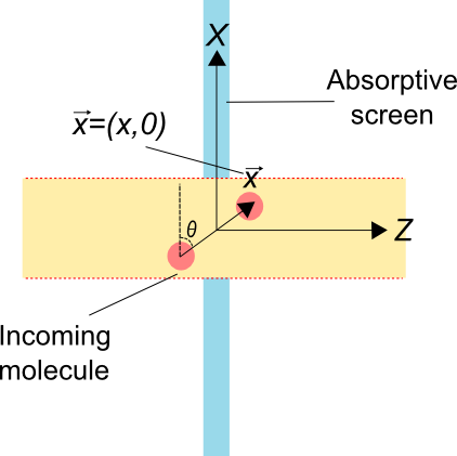
Figure 3: The allowed region is the shaded area between dashed lines when $Z=0$.

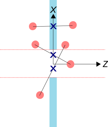
Figure 4: Cases regarded as absorption include one or both particles outside the allowed region when $Z=0$.

From (22) and (23) it is evident that intramolecular degrees of freedom are entangled with the center of mass momentum $\vec{P}=\hbar\vec{K}$ appearing as integration variable; this is a fundamental property to consider when we seek visible changes in the diffraction pattern beyond point-like structures. For example, if we had $\psi_{0}(X^{\prime},r^{\prime},\theta^{\prime})=\psi(X^{\prime})\phi_{n_{0}l_{0}}(r^{\prime},\theta^{\prime})$ in (14) then the solution would be separable in relative and center-of-mass coordinates in all regions, leading to full disentanglement and a trivial expression for (21), as we anticipated in II.2. In general, an opaque screen will produce non-trivial superpositions and therefore an entangled relative and center-of-mass motion. Now, we impose the requirement that particles occupy only the empty region of the grate when $Z=0$, i.e. between the limits defined by the edges of the screen, as shown in fig. 3. Any other case will be regarded as an absorption event, and therefore shall not contribute to the probability density at the other side. In order for the wave function to fulfill these restrictions, illustrated in fig. 3 and 4, and simultaneously represent an incoming molecular state of a well-defined internal energy, the following product is to be considered:

$$\psi_{0}(X^{\prime},r^{\prime},\theta^{\prime})=\mathcal{N}\Theta\left(\frac{L}{2}-|x_{1}^{\prime}|\right)\Theta\left(\frac{L}{2}-|x_{2}^{\prime}|\right)\phi_{n_{0}l_{0}}(r^{\prime},\theta^{\prime}).$$ (24)

Here, the Heaviside $\Theta$ functions truncate the incoming wave and the absence of additional plane wave factors indicate normal incidence of the beam; the factor $\mathcal{N}$ is a normalization constant that from now on will be omitted, and $L$ is the width of the slit. From a physical point of view, the molecule can be introduced in a single state from a source at the left, as shown by recent investigations chouPreparationCoherentManipulation2017b on the preparation and coherent manipulation of molecular ions. According to the change of variables in (3), the function (24) is

$$\begin{split}\psi_{0}(X^{\prime},r^{\prime},\theta^{\prime})&=\Theta\left(\frac{L}{2}-|X^{\prime}-\frac{m_{2}x^{\prime}}{M}|\right)\\ &\times\Theta\left(\frac{L}{2}-|X^{\prime}+\frac{m_{1}x^{\prime}}{M}|\right)\\ &\times\phi_{n_{0}l_{0}}(r^{\prime},\theta^{\prime})\\ &=\Theta\left(\frac{L}{2}-|X^{\prime}-\frac{m_{2}r^{\prime}\text{cos}\theta^{\prime}}{M}|\right)\\ &\times\Theta\left(\frac{L}{2}-|X^{\prime}+\frac{m_{1}r^{\prime}\text{cos}\theta^{\prime}}{M}|\right)\\ &\times\phi_{n_{0}l_{0}}(r^{\prime},\theta^{\prime}),\end{split}$$ (25)

and it is not separable as a product in relative and center-of-mass coordinates, as expected.

II.5 Solutions in series expansion for small molecules

For ease of exposition in further developments, we introduce here some definitions related to Moshinsky functions moshinskyDiffractionTime1952 ; faddeevaTablesValuesFunction1961 ; corderoDiffractionTimeTunneling2013 , which come from the truncated integration of imaginary Gaussian kernels arising in the problem of diffraction by edges. We start with

$$\begin{split}&M(X,Z,r^{\prime},\theta^{\prime};E-\epsilon_{nl})\equiv\\ &\int_{-\infty}^{\infty}dX^{\prime}K(X-X^{\prime},Z;E-\epsilon_{nl})\psi_{0}(X^{\prime},r^{\prime},\theta^{\prime}).\\ \end{split}$$ (26)

Substitution of this expression in the wavefunction, according to (14) and (16), yields

$$\begin{split}&\psi(X,Z,r,\theta)=\\ &\sum_{nl}\int r^{\prime}dr^{\prime}d\theta^{\prime}\phi^{*}_{nl}(r^{\prime},\theta^{\prime})\phi_{nl}(r,\theta)M(X,Z,r^{\prime},\theta^{\prime};E-\epsilon_{nl}).\end{split}$$ (27)

A proper care of the initial condition at the screen (25) in terms of the center of mass $X$ implies variable boundaries for the integration variable $X^{\prime}$. This leads to the limits

$$\begin{split}-\frac{L}{2}+\frac{m_{2}r^{\prime}\text{cos}\theta^{\prime}}{M}&<X^{\prime}<-\frac{m_{1}r^{\prime}\text{cos}\theta^{\prime}}{M}+\frac{L}{2}\\ -\frac{L}{2}-\frac{m_{1}r^{\prime}\text{cos}\theta^{\prime}}{M}&<X^{\prime}<\frac{m_{2}r^{\prime}\text{cos}\theta^{\prime}}{M}+\frac{L}{2},\end{split}$$

and by using the following shorthands

$$\begin{split}S_{-}(\theta^{\prime};m_{1},m_{2})&\equiv\text{max}\left(\frac{m_{2}\text{cos}\theta^{\prime}}{M},-\frac{m_{1}\text{cos}\theta^{\prime}}{M}\right)\\ S_{+}(\theta^{\prime};m_{1},m_{2})&\equiv\text{min}\left(\frac{m_{2}\text{cos}\theta^{\prime}}{M},-\frac{m_{1}\text{cos}\theta^{\prime}}{M}\right)\\ X_{\pm}(r^{\prime},\theta^{\prime};m_{1},m_{2})&\equiv r^{\prime}S_{\pm}(\theta^{\prime};m_{1},m_{2})\pm\frac{L}{2}\\ \\ \\ \\ \end{split}$$ (28)

the expression (LABEL:Moshinsky_function) can be recast as

$$\begin{split}&M(X,Z,r^{\prime},\theta^{\prime};E-\epsilon_{nl})=\\ \phi_{n_{0}l_{0}}(r^{\prime},\theta^{\prime})&\int_{X_{-}(r^{\prime},\theta^{\prime},m_{1},m_{2})}^{X_{+}(r^{\prime},\theta^{\prime},m_{1},m_{2})}dX^{\prime}K(X-X^{\prime},Z;E-\epsilon_{nl}).\end{split}$$ (29)

It is convenient to further define the two single-edge functions $M_{\pm}$ as

$$\begin{split}&M_{\pm}(X,Z,r^{\prime},\theta^{\prime};E-\epsilon_{nl})\equiv\\ &\int_{X_{\pm}(r^{\prime},\theta^{\prime},m_{1},m_{2})}^{\infty}dX^{\prime}K(X-X^{\prime},Z;E-\epsilon_{nl}),\end{split}$$ (30)

and with this, (LABEL:Moshinsky_function_variable_limits) acquires the form:

$$\begin{split}&M(X,Z,r^{\prime},\theta^{\prime};E-\epsilon_{nl})=\phi_{n_{0}l_{0}}(r^{\prime},\theta^{\prime})\times\\ &\times\left[M_{-}(X,Z,r^{\prime},\theta^{\prime};E-\epsilon_{nl})-M_{+}(X,Z,r^{\prime},\theta^{\prime};E-\epsilon_{nl})\right].\end{split}$$ (31)

Now we proceed to evaluate the integral in (LABEL:Moshinsky_min_max_function). This can be done by considering a Taylor series for small values of $r^{\prime}$. Since the limits in (28) are linear in $r^{\prime}$, multiple derivatives with respect to this variable are easy to obtain; therefore, we shall be able to evaluate all terms in the series explicitly. As a preliminary step, we need to re-express (LABEL:Moshinsky_min_max_function) by displacing $X$ with a change of variables in the integrals $X^{\prime}\mapsto X^{\prime}\pm L/2$:

$$\begin{split}&M_{\pm}(X\pm L/2,Z,r^{\prime},\theta^{\prime};E-\epsilon_{nl})=\\ &\int_{r^{\prime}S_{\pm}(\theta^{\prime},m_{1},m_{2})}^{\infty}dX^{\prime}K(X-X^{\prime},Z;E-\epsilon_{nl}).\end{split}$$ (32)

With this, the Taylor series reads:

$$\begin{split}M_{\pm}(X\pm L/2,Z,r^{\prime},\theta^{\prime};E-\epsilon_{nl})&=\sum_{k=0}^{\infty}\frac{(r^{\prime})^{k}}{k!}\left[\left(\frac{\partial}{\partial r^{\prime\prime}}\right)^{(k)}M_{\pm}(X\pm L/2,Z,r^{\prime\prime},\theta^{\prime};E-\epsilon_{nl})\right]_{r^{\prime\prime}=0}\\ &=\sum_{k=0}^{\infty}\frac{(r^{\prime})^{k}}{k!}(S_{\pm})^{k}\left(\frac{\partial}{\partial X}\right)^{(k)}M_{\pm}(X\pm L/2,Z,0,\theta^{\prime};E-\epsilon_{nl}).\\ \end{split}$$ (33)

Notably, the first term of the sum corresponds to the Moshinsky function of a structureless particle, the second is its derivative, i.e. the free propagator, and the following terms are higher derivatives of the free propagator, which are known functions. Although all the terms in the series can be evaluated, we shall consider only the first power of $r^{\prime}$. We present an argument for the truncability of the series in appendix A.

With these considerations, (33) becomes

$$\begin{split}&M_{\pm}(X\pm L/2,Z,r^{\prime},\theta^{\prime};E-\epsilon_{nl})=\\ &\int_{0}^{\infty}dX^{\prime}K(X-X^{\prime},Z;E-\epsilon_{nl})\\ &+r^{\prime}K(X,Z;E-\epsilon_{nl})S_{\pm}(\theta^{\prime};m_{1},m_{2})+\mathcal{O}^{2}\left(r^{\prime}\right).\end{split}$$ (34)

The small correction $\mathcal{O}^{2}\left(r^{\prime}\right)$ can be shown to be $\mathcal{O}^{2}\left(\frac{a}{L},\frac{\lambda}{Z}\right)$ in terms of the width of the slit $L$ and the characteristic length $a$ of the molecule, as discussed also in appendix A. From (28) and (LABEL:Moshinsky_min_max_function) we have

$$\begin{split}&M_{\pm}(X\pm L/2,Z,r^{\prime},\theta^{\prime};E-\epsilon_{nl})=\\ &M_{0}(X,Z;E-\epsilon_{nl})-r^{\prime}S_{\pm}(\theta^{\prime},m_{1},m_{2})K(X,Z;E-\epsilon_{nl}),\end{split}$$ (35)

where

$$M_{0}(X,Z;E-\epsilon_{nl})=\int_{0}^{\infty}dX^{\prime}K(X-X^{\prime},Z;E-\epsilon_{nl})$$ (36)

is the usual Moshinsky function with one edge placed at the origin. One remarkable achievement in (LABEL:displaced_Moshinsky_min_max_function_expanded) is that we have successfully identified the intramolecular corrections to the center of mass propagation, which will prove useful later on. Moreover, we may reverse the displacement done in (LABEL:Moshinsky_min_max_function_displaced) in order to recover the dependence on $X$ alone:

$$\begin{split}&M_{\pm}(X,Z,r^{\prime},\theta^{\prime};E-\epsilon_{nl})=M_{0}(X\mp L/2,Z;E-\epsilon_{nl})\\ &-r^{\prime}S_{\pm}(\theta^{\prime},m_{1},m_{2})K(X\mp L/2,Z;E-\epsilon_{nl}).\end{split}$$ (37)

Finally, we build a combination of functions for each edge at $X=\pm L/2$ in order to get the single-slit function:

$$\begin{split}&M_{L}(X,Z,r^{\prime},\theta^{\prime};E-\epsilon_{nl})\equiv\\ &M_{0}(X+L/2,Z;E-\epsilon_{nl})-M_{0}(X-L/2,Z;E-\epsilon_{nl}),\end{split}$$ (38)

and by means of (LABEL:Moshinsky_function_min-max), our Moshinsky function with molecular degrees of freedom (LABEL:Moshinsky_function) becomes

$$\begin{split}&M(X,Z,r^{\prime},\theta^{\prime};E-\epsilon_{nl})=M_{L}(X,Z;E-\epsilon_{nl})\phi_{n_{0}l_{0}}(r^{\prime},\theta^{\prime})\\ &-[r^{\prime}S_{-}(\theta^{\prime},m_{1},m_{2})K(X+L/2,Z;E-\epsilon_{nl})\\ &-r^{\prime}S_{+}(\theta^{\prime},m_{1},m_{2})K(X-L/2,Z;E-\epsilon_{nl})]\phi_{n_{0}l_{0}}(r^{\prime},\theta^{\prime}).\end{split}$$ (39)

This, together with the specific form of the molecular functions (9), allows to calculate the full wave function (LABEL:general_solution_explicit):

$$\begin{split}&\psi(X,Z,r,\theta)=\phi_{n_{0}l_{0}}(r,\theta)M_{L}(X,Z;E-\epsilon_{n_{0}l_{0}})\\ &-\sum_{nl}\phi_{nl}(r,\theta)\times\\ &\times\left[\right.\bra{nl}\left\|r^{\prime}\right\|\ket{n_{0}l_{0}}f_{ll_{0}}(m_{1},m_{2})K(X+L/2,Z;E-\epsilon_{nl})\\ &-\bra{nl}\left\|r^{\prime}\right\|\ket{n_{0}l_{0}}g_{ll_{0}}(m_{1},m_{2})K(X-L/2,Z;E-\epsilon_{nl})\left.\right].\end{split}$$ (40)

In this expression, we see that the expansion coefficients involve reduced matrix elements $\langle|\left\|r^{\prime}\right\||\rangle$ of the relative radius, i.e.

$$\bra{nl}\left\|r^{\prime}\right\|\ket{n_{0}l_{0}}=\int_{0}^{\infty}r^{\prime 2}dr^{\prime}R^{*}_{nl}(r^{\prime})R_{n_{0}l_{0}}(r^{\prime})$$ (41)

$$f_{ll_{0}}(m_{1},m_{2})=\int_{0}^{2\pi}d\theta^{\prime}S_{-}(\theta^{\prime};m_{1},m_{2})e^{-il\theta^{\prime}}e^{il_{0}\theta^{\prime}}$$ (42)

$$g_{ll_{0}}(m_{1},m_{2})=\int_{0}^{2\pi}d\theta^{\prime}S_{+}(\theta^{\prime};m_{1},m_{2})e^{-il\theta^{\prime}}e^{il_{0}\theta^{\prime}}.$$ (43)

An explicit calculation of (42) and (43), which can be seen in appendix B, leads to

$$f_{ll_{0}}(m_{1},m_{2})=f_{ll_{0}}=\zeta_{l-l_{0}}\left[\frac{2}{1-(l-l_{0})^{2}}\right]$$ (44)

$$\zeta_{n}\equiv\text{cos}\left(\frac{\pi}{2}n\right)=\begin{cases}1&n=0,4,8...\\ 0&n=1,3,5...\\ -1\;\;\;\;&n=2,6,10...\end{cases}$$ (45)

$$g_{ll_{0}}=-f_{ll_{0}}\hskip 56.9055pt$$ (46)

or more explicitly,

$$f_{ll_{0}}=\begin{cases}\frac{2}{1-(l_{0}-l)^{2}}&l=l_{0},l_{0}\pm 4,l_{0}\pm 8...\\ 0&l=l_{0}\pm 1,l_{0}\pm 3,l_{0}\pm 5...\\ \frac{2}{(l_{0}-l)^{2}-1}\;\;\;\;&l=l_{0}\pm 2,l_{0}\pm 6,l_{0}\pm 10...\end{cases}\vspace{0.1cm}$$ (47)

These coefficients are independent of physical parameters, such as mass, wavelength, etc. Their contribution can be estimated merely on numerical grounds, so only a few of them around the initial angular momentum $l_{0}$ contribute effectively. We also see that the central relation in (47) states the conservation of parity in the diffractive process. Indeed, under space inversion, the wave function in polar coordinates changes the phase factor as

$$\psi_{nl}(-\vec{r})=(-1)^{l}\psi_{nl}(\vec{r}),$$ (48)

and from parity conservation, $l$ must remain even or odd, acting as a selection rule for the states that the diffractive plate can entangle on the right hand side of the geometry. In particular, $l$ cannot take the value $l=l_{0}+1$, a prohibition that avoids the singularity in the denominator of (47).

As a final stage of our mathematical considerations, we provide now an explicit form of the marginal probability density, previously defined. Using the abbreviation

$$\begin{split}&K_{L}(X,Z;E-\epsilon_{nl})\equiv\\ &K(X+L/2,Z;E-\epsilon_{nl})+K(X-L/2,Z;E-\epsilon_{nl})\end{split}$$ (49)

we can express the marginal probability density (21) in a neat form:

$$\begin{split}|\rho(X,Z;E-\epsilon_{n_{0}l_{0}})|^{2}&=|M_{L}(X,Z;E-\epsilon_{n_{0}l_{0}})|^{2}-2\text{Re}[\bra{n_{0}l_{0}}\left\|r^{\prime}\right\|\ket{n_{0}l_{0}}f_{l_{0}l_{0}}K_{L}(X,Z;E-\epsilon_{n_{0}l_{0}})M^{*}_{L}(X,Z;E-\epsilon_{n_{0}l_{0}})]\\ &+\sum_{nl}|\bra{nl}\left\|r^{\prime}\right\|\ket{n_{0}l_{0}}|^{2}|f_{ll_{0}}|^{2}|K_{L}(X,Z;E-\epsilon_{nl})|^{2}.\end{split}$$ (50)

Once more, we find a dominant term corresponding to a structureless particle, plus corrections containing various matrix elements of the molecular radius. A useful comparison between these contributions can be made.

III Application to the harmonic molecular model

In this section, we obtain explicit formulas for wave functions and marginal distributions in the case of a quadratic interaction between atoms. For simplicity we use a harmonic oscillator, assuming equidistant energy states, and a characteristic molecular length given in terms of the oscillator strength. We shall see how this system provides revivals in the diffraction pattern, as extensively studied for wavepackets, even for anharmonic systems vrakkingObservationFractionalRevivals1996 . On the other hand, realistic models of molecules may posses irregular spectra, and may even have a dissociation tendency that calls for scattering (unbound) states. For solvable molecular models of this kind, see leeModifiedMorsePotential1998 ; shoreComparisonMatrixMethods1973 ; berrondoAlgebraicApproachMorse1980 ; infeldFactorizationMethod1951 . However, as we stated in (26), those limits are outside of the scope and shall be studied elsewhere.

III.1 Explicit computations

For the integration in (36) we may use the exact expression of the propagator (LABEL:propagator_graphics_exact), but considering small molecular radii and the paraxial approximation (LABEL:propagator_graphics_paraxial) in the propagation of the center of mass. We employ the following form of (36)

$$\begin{split}M_{0}(X,Z,E-\epsilon_{n_{0}l_{0}})\approx\sqrt{\frac{-i}{2}}e^{i\sqrt{\frac{2M}{\hbar^{2}}(E-\epsilon_{n_{0}l_{0}})}Z}\left[\frac{1}{2}+\frac{i}{2}+C\left(\sqrt{\frac{\sqrt{\frac{2M}{\hbar^{2}}(E-\epsilon_{n_{0}l_{0}})}}{Z\pi}}X\right)+iS\left(\sqrt{\frac{\sqrt{\frac{2M}{\hbar^{2}}(E-\epsilon_{n_{0}l_{0}})}}{Z\pi}}X\right)\right]\end{split}$$ (51)

with $C(x)$ and $S(x)$ the Fresnel functions. Now we introduce the harmonic oscillator radial functions; see e.g. karimiRadialQuantumNumber2014a :

$$\begin{gathered}R_{nl}(r)=\sqrt{\beta}\sqrt{\frac{2n!}{(n+|l|)!}}\left(\sqrt{\beta}r\right)^{|l|}e^{-\beta r^{2}/2}L_{n}^{|l|}(\beta r^{2})\\ \beta=\frac{\omega\mu}{\hbar},\end{gathered}$$ (52)

where $L_{n}^{|l|}(x)$ are the associated Laguerre polynomials and $\omega$ is the frecuency. The constant $\beta$ matches our expectations, as we identify now a constant $a$ with the characteristic length of the molecule

$$a=1/\sqrt{\beta}=\sqrt{\frac{\hbar}{\omega\mu}}.$$ (53)

The internal energy is given by

$$\begin{split}\epsilon_{nl}&=(2n+|l|+1)\epsilon_{00}\\ \epsilon_{00}&=\hbar\omega=\frac{\hbar^{2}}{a^{2}\mu}.\end{split}$$ (54)

With the intention of evaluating (41) we recall the explicit expansion of associated Laguerre polynomials

$$L_{n}^{|l|}(r)=\sum_{k=0}^{n}C^{n|l|}_{k}r^{k},$$ (55)

where the coefficients $C^{n|l|}_{k}$ can be consulted in abramowitzHandbookMathematicalFunctions2013 . Now we can write the product of associated Laguerre polynomials $L_{n}^{|l|}(u^{2})L_{n_{0}}^{|l_{0}|}(u^{2})$ as a series of even powers of $u$:

$$L_{n}^{|l|}(u^{2})L_{n_{0}}^{|l_{0}|}(u^{2})=\sum_{k=0}^{n+n_{0}}\left[\sum_{a,b\,:\,a+b=k}C^{n_{0}|l_{0}|}_{a}C^{n|l|}_{b}\right]u^{2k}.$$ (56)

With a change of variables, the reduced matrix elements of the molecular radius (41) can be expressed as:

$$\bra{nl}\left\|r^{\prime}\right\|\ket{n_{0}l_{0}}=a\sum_{k=0}^{n+n_{0}}D_{k}\text{T}\left(k+\frac{1}{2}|l|+\frac{1}{2}|l_{0}|\right),$$ (57)

and here the coefficients $D_{k}$ are known in terms of $C$

$$D_{k}=\sqrt{\frac{2n!}{(n+|l|)!}}\sqrt{\frac{2n_{0}!}{(n_{0}+|l_{0}|)!}}\left[\sum_{a,b\,:\,a+b=k}C^{n_{0}|l_{0}|}_{a}C^{n|l|}_{b}\right].$$ (58)

In (57) we also introduced the Talmi integral $\text{T}(k)$, frequently employed in nuclear physics:

$$\text{T}(p)=\int_{0}^{\infty}e^{-u^{2}}u^{2p+2}du,$$ (59)

which can be put in terms of gamma functions; from (47) we note that the argument of T in (57) is an integer. This guarantees that all terms in the expansion (50) can be evaluated for general values of incoming quantum numbers $n_{0},l_{0}$. In particular, for the ground state of the molecule $n_{0}=l_{0}=0$ we have

$$\begin{split}\bra{nl}\left\|r^{\prime}\right\|\ket{0,0}=a\frac{\Gamma(n+\frac{|l|}{2}-\frac{1}{2})}{4\Gamma(n+1)}(l^{2}-1)\sqrt{\frac{n!}{(n+|l|)!}}.\\ \end{split}$$ (60)

We can verify that (60) goes to zero as $n$ increases with $l$ fixed, e.g., $2\pi\bra{0,0}\left\|r^{\prime}\right\|\ket{0,0}/a=\sqrt{\pi}/2$ and $2\pi\bra{3,0}\left\|r^{\prime}\right\|\ket{0,0}/a=-\sqrt{\pi}/32$. In general, we expect a decaying coefficient by looking at fig. 15: the greater the number of nodes (which is determined by $n$) the smaller the integral in (60).

III.2 Specific cases

In what follows, we put all space variables in (50) as quotients relative to the slit width $L$.

Now we apply (50) to specific molecular dimensions. In the near field region, i.e. close to the slit, we shall use the exact form of the propagator (LABEL:propagator_graphics_exact). In order to describe a particular diatomic molecule, we only need to specify the values of the parameters in (52) and (54). Our interest is to obtain visible effects emerging from certain molecular features, such as mass asymmetry, non-negligible radius and incident energy. Particular values for existing molecules can be found in different sources, e.g. huberMolecularSpectraMolecular2013 .
Let us consider a case of small asymmetry, where

$$\begin{split}m_{1}&=20\text{u}\\ m_{2}&=26\text{u},\end{split}$$ (61)

and u is the molecular mass unit. Now we can vary the ratios $\lambda/L$ and $a/L$ for some representative cases corresponding to different molecular scales. A notable focusing effect is known to appear in the intermediate region of the pattern; we show the modifications produced by the internal structure in this case. Lastly, we present the calculation of the diffraction pattern of multiple slits, giving rise to a quantum carpet of a point-like particle and a diatomic molecule, as those shown in fig. 1.

Near field

In our investigations, we have found that the differences between patterns with and without internal structure are more noticeable in the near field. A long wavelength makes the effect more conspicuous. This is shown in fig. 5, where a close look into the diffraction pattern along the propagation axis can be taken. The parameters used are the following:

$$\begin{split}\lambda/L&=9.64\times 10^{-5}.\end{split}$$ (62)

We vary $a/L$ as indicated in the figure, where $a/L=0$ gives the point-like particle diffraction pattern. These values extend to molecules as large as 1/1000 the size of the slit. The purple curve in 5 has an envelope with an anomalous spike, when only the first correction in the series is employed.

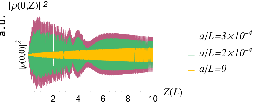
Figure 5: The effect that arises in the diatomic molecule diffraction is more present in the near field, the parameters used in these patterns are specified in (62).

Optic grate

The diffraction of matter waves due to the interaction with a classical electromagnetic wave of a short wavelength is known as the Kapitza-Dirac effect. If we model the potential created by such a stationary wave as a hard wall, we may find that $L$ stands for half a wavelength. In this scenario, we are interested in the displacement of the focusing point, i.e. the largest maximum, as a function of $a$. We hope that this shift can be detected using current technology. We consider the following values in the diffraction via the optic grate:

$$\begin{split}\lambda/L&=3.89\times 10^{-4}\\ a/L&=4\times 10^{-3},\end{split}$$ (63)

which represent a reasonable kinetic energy for a molecular beam, and a minute but non-negligible molecular radius. In fig. 6 we see the diffraction pattern along the propagation axis, where the focusing point is almost the same in both cases; we can make the difference more clear with other parameters, as illustrated below.

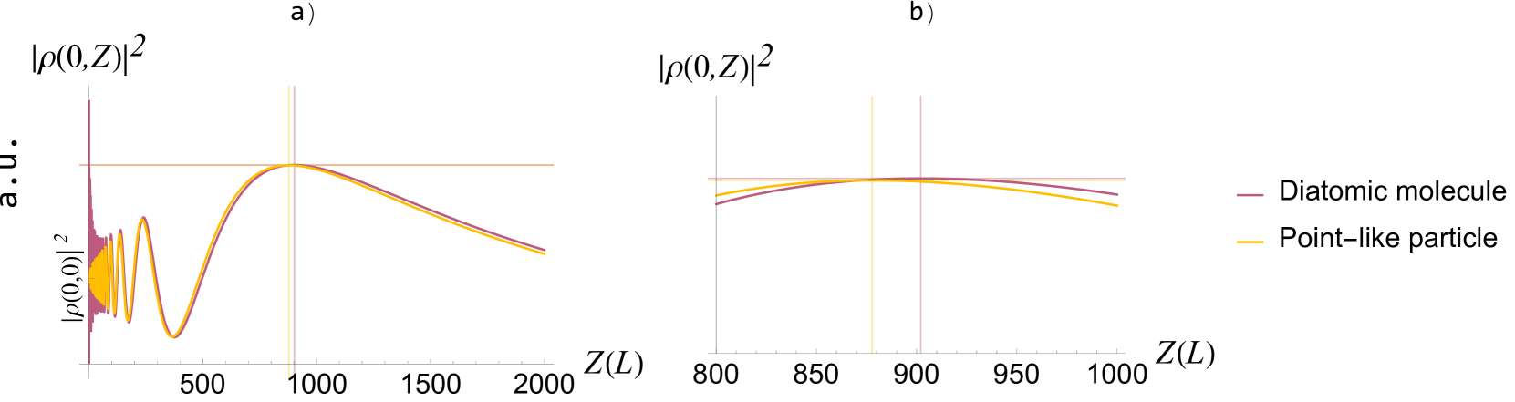
Figure 6: Small deviations of the focusing point at $Z=1380L$. In a) we see that the global effect, which is more noticeable around $Z=0$, in b) we show a magnification of the peak; vertical lines mark the exact position of the maximum. Parameters: $\lambda/L=3.89\times 10^{-4}$ and $a/L=0.004$.

Nano structure

The effect of $a$ on the diffraction pattern is more evident if we reduce the size of the grate. We can achieve this by considering a nanostructure, which corresponds to the following parameters:

$$\begin{split}\lambda/L&=9.64\times 10^{-4}\\ a/L&=0.14.\end{split}$$ (64)

The resulting pattern in fig. 7 has far more prominent deviations. A cautionary remark is in order: The near field deviations are to large to be considered corrections, so more terms in the power series of the radius must be included.

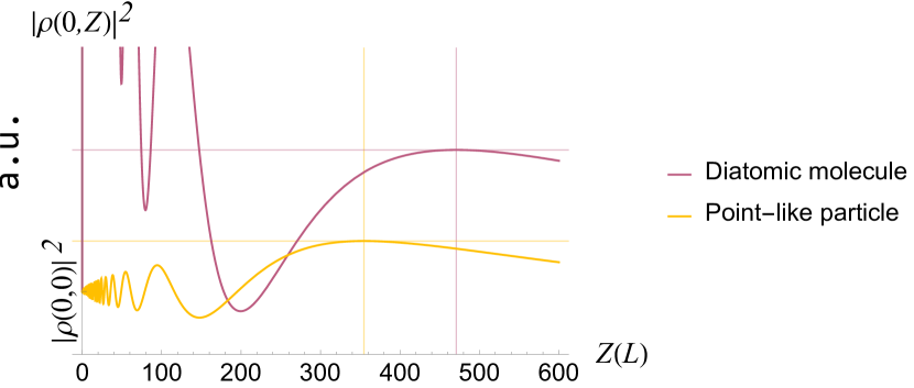
Figure 7: The displacement of the focusing point is caused by a large contribution of the terms in (50) containing $a/L$. The pattern at $Z=0$ has a larger intensity, but it does not diverge. Parameters: $\lambda/L=9.64\times 10^{-4}$ and $a/L=0.14$.

Crystalline structure

Lastly, we present the diffraction by a crystalline structure with very fine grating. Here, the displacement of the focusing point is more noticeable. Although it is an experimental challenge to detect molecular diffraction by crystals ($L$ is now in the atomic scale) we may substitute numbers to get an idea. We do not discard the possibility that thin sheets of periodic structures such as graphene can used as gratings, provided the energy of the projectile does not compromise the crystal itself. The parameters used are

$$\begin{split}\lambda/L&=0.363\\ a/L&=0.335,\end{split}$$ (65)

This pattern is shown in fig. 8. A similar comment on small corrections applies here: the firs few terms of the series may had lost validity as the differences are very prominent, even in the far field. However, the change in the curves has a gradual development in $a/L$, as can be seen in fig. 9. Particular attention to the green line for $a/L=0.15$ should be paid. As the validity of small corrections in (50) is ensured, we conclude here that a finite radius increases the focus and deepens the minimum, producing a stronger contrast in the midfield pattern.

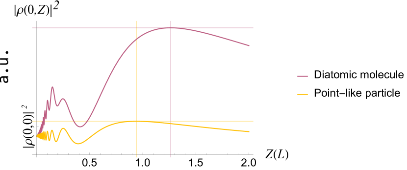
Figure 8: This pattern results from a very fine grate. Parameters: $\lambda/L=0.363$ and $a/L=0.335$. These are the largest molecular realizations of the present paper. The approximation (50) eventually fails when $a/L$ increases further.

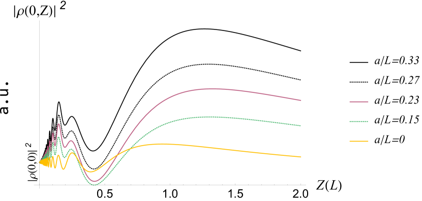
Figure 9: Change of the diffraction pattern as the molecular radius increases.

IV Diffraction by periodic slits and Talbot carpets

We can easily expand our results to the case of a periodic diffraction grating if we consider the superposition of (25) a given number of times $N$. To this end we introduce a subscript $N$ in our notation:

$$\psi_{0}(X^{\prime},r^{\prime},\theta^{\prime})_{N}=\sum_{k=-N}^{N}\psi_{0}(X^{\prime}+kd,r^{\prime},\theta^{\prime}).$$ (66)

Here, $d$ is the separation between each slit. From geometric considerations, it is clear that we need $d>L$. This initial condition at $Z=0$ for multiple slits will result in a superposition of wave functions of the form (LABEL:general_solution_calculated):

$$\psi(X,Z,r,\theta)_{N}=\sum_{k=-N}^{N}\psi(X+kd,Z,r,\theta).$$ (67)

From this wave function, we can easily derive the marginal probability density in a way that is analogous to (50)

$$\begin{split}&|\rho(X,Z;E-\epsilon_{n_{0}l_{0}})|^{2}_{N}=|M_{L}(X+kd,Z;E-\epsilon_{n_{0}l_{0}})_{N}|^{2}\\ &-2\text{Re}[\bra{n_{0}l_{0}}\left\|r^{\prime}\right\|\ket{n_{0}l_{0}}f_{l_{0}l_{0}}\times\\ &\times K_{L}(X,Z;E-\epsilon_{n_{0}l_{0}})_{N}M^{*}_{L}(X,Z;E-\epsilon_{n_{0}l_{0}})_{N}]\\ &+\sum_{nl}|\bra{nl}\left\|r^{\prime}\right\|\ket{n_{0}l_{0}}|^{2}|f_{ll_{0}}|^{2}|K_{L}(X,Z;E-\epsilon_{nl})_{N}|^{2},\end{split}$$ (68)

where we used (LABEL:Moshinsky_0_+-) and (LABEL:propagator_+-) to define:

$$M_{L}(X,Z;E-\epsilon_{n_{0}l_{0}})_{N}=\sum_{k=-N}^{N}M_{L}(X+kd,Z;E-\epsilon_{n_{0}l_{0}})$$ (69)

$$K_{L}(X,Z;E-\epsilon_{nl})_{N}=\sum_{k=-N}^{N}K_{L}(X+kd,Z;E-\epsilon_{nl}).$$ (70)

By taking the limit $N\rightarrow\infty$, we obtain a truly periodic array of slits and thus, we expect that $|\rho|^{2}_{N}$ to represent what is known as a Talbot carpettalbotLXXVIFactsRelating1836a . Instead of light waves berryQuantumCarpetsCarpets2001 or atomic beams, the carpets are made of molecular waves.

$$|\rho(X,Z;E-\epsilon_{n_{0}l_{0}})|^{2}_{T}=\lim\limits_{N\to\infty}|\rho(X,Z;E-\epsilon_{n_{0}l_{0}})|^{2}_{N}.$$ (71)

One crucial characteristic of Talbot carpets we manage to reproduce here is the periodicity of their revivals, as we now discuss.

Diffraction patterns in molecular Talbot carpets

For finite values of $N$, the diffraction patterns obtained will be more accurate in the region near the central slits, therefore we consider values

$$\begin{split}X/d&\sim 1\\ Z/L_{T}&\sim 1,\end{split}$$ (72)

where $L_{T}$ is the Talbot length, primary revivals take place at multiples of this length, secondary revivals occur at multiples of $L_{T}/2$. In our computations, we find that for a point-like particle $L_{T}$ is given by

$$L_{T}=\frac{2d^{2}}{\lambda}.$$ (73)

We use (LABEL:Talbot_marginal_probability_density) with $N=20$ to compare the diffraction patterns of a point-like particle and a diatomic molecule; the separation between each slit was made eight times their length:

$$\begin{split}d=8L.\end{split}$$ (74)

In fig. 10 we show the probability density along the $Z$ axis at $X=d/2$ for the case of an optical grating, using parameters (63) for the molecule. We find that differences are hardly noticeable around the region of the secondary revival; in contrast, in fig. 11 we show the diffraction pattern around the same region for the case of a nano structure, obtained with parameters (64) for the molecule, and producing more prominent changes. As expected, the case of a crystalline structure presents the largest differences between patterns.

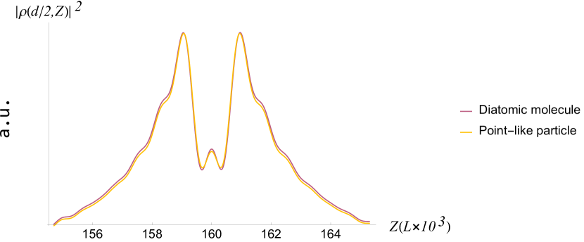
Figure 10: Diffraction patterns due to a periodic grating along the $Z$ axis displaced at $X=d/2$. The region around the first secondary revival ($Z=1/2L_{T}$) is shown for two cases, but differences are hardly noticeable for parameters (63).

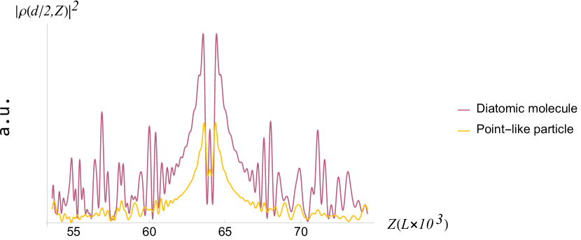
Figure 11: Diffraction patterns due to a periodic grating along the $Z$ axis displaced at $X=d/2$. Now, the region around the first secondary revival ($Z=1/2L_{T}$) displays visible changes for the case of a nano structure, according to parameters (64) for the molecule.

We show various regions for the case of a crystalline structure using parameters (65). In fig. 12 we see the comparison in a panoramic view along various revivals; then we specialize in fig. 13 to some regions.

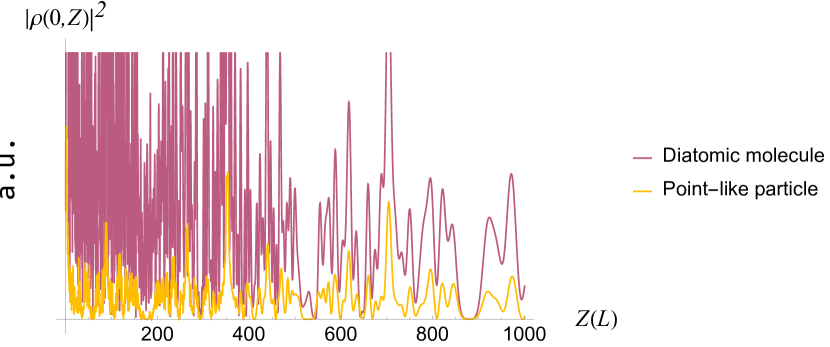
Figure 12: Diffraction pattern on a large portion along the propagation axis. Using the parameters (65) for the molecule in eq. (LABEL:Talbot_marginal_probability_density) we find once more that the largest differences take place in the near field.

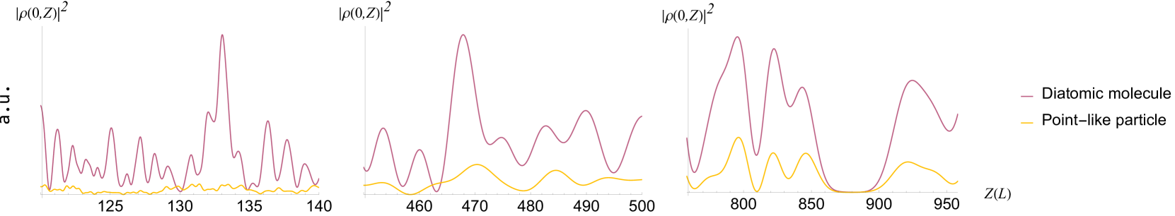
Figure 13: Magnifications of the near, intermediate and far regions, respectively of fig. 12.

Finally, in fig. 14 we present a comparison between the diffraction of a single slit, where we show the pattern of the point-like particle (left panel) the diatomic correction term alone (central panel) and the pattern of the diatomic molecule (right panel). To complete the circle, in fig. 1 we show a comparison of two Talbot carpets for a point-like particle and the diatomic harmonic molecule.

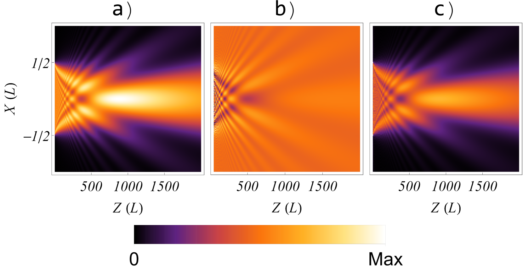
Figure 14: Using (50) and parameters $\lambda/L=3.89\times 10^{-4}$ and $a/L=0.004$ we obtain a) the pattern without molecular correction, b) the second and third terms of (50) as a visual aid to the influence of the molecular structure, and c) the full expression (50) where the changes are mostly visible in the near field caseDiffractiveMechanismFocusing2012 .

V Conclusions

Our theoretical description of propagation for composite particles has been successful in reproducing the correction due to internal structure in all regions of space (50). This treatment is not limited to transmission and reflection coefficients –typical of scattering theory– recovered with integrals of waves in the far region. Although we used an approximation to first order in the molecular radius $a/L$ for ease in the calculations, our results (33) and (LABEL:displaced_Moshinsky_function_variable_limits_expanded) contain all the terms in the expansion and we have shown how to evaluate them by application of successive derivatives with respect to the transverse coordinate $X$. For molecules with large radii we can always resort to (LABEL:Moshinsky_min_max_function_displaced) and proceed with numerical evaluations. For definiteness, we introduced a harmonic interaction between atoms. It is remarkable that the internal structure makes its appearance in the radial wave functions alone, opening thus the possibility of studying more complex models by merely modifying the wave functions; for instance, it would be possible to introduce plasticity or dissociation at this level, understood as a set of waves which contain both a limited number of bound states for low internal energies and an infinite number of scattering states that represent two free particles in the radial coordinate.

Regarding the differences in the diffraction patterns, in fig. 14 we appreciate how the effects due to the internal structure are hardly noticeable in the far field, but as can be seen in fig. 5, the correction is imperative in the near field, as the molecular effect changes the intensity peaks. An additional observation that can be done regarding (50) is that diffraction binds together different states of the molecule and, together with the selection rule in $f_{ll_{0}}$, it leads to entanglement of states $|n,l\rangle$, as confirmed by the analysis of the resulting wave function (LABEL:general_solution_calculated). As an outlook, our analytical results can also be employed in the study of entanglement between the center of mass and relative degrees of freedom, at various points along the optical axis. Although no attempt has been made in this work to define the entropy of a diffracted wave function, we anticipate that partial tracing of relative coordinates and the computation of von Neuman’s entropy at various slices of $Z$ will support the view that diffractive effects can be associated with disorder.

Appendix A Truncability of the series

It is not too audacious to make an expansion series on the molecular radius: as we can infer from square integrability, eq. (10), when $r^{\prime}\rightarrow\infty$, $\phi(r^{\prime},\theta^{\prime})\rightarrow 0$ sufficiently fast. This ensures a finite result (see fig. 15) for each coefficient and helps the convergence of the series. We also argue that the molecular function only “sees” the vicinity of the grate at $Z=0$ due to a finite radius; this has an influence on (LABEL:Moshinsky_function_variable_limits) and subsequent terms in the series. This approach can be used for internal wave functions with bound states, as the probability density vanishes for large separation distances; however, if the wave function is appreciable as $r^{\prime}\rightarrow\infty$, the approximation becomes invalid, i.e. a problem with molecular dissociation. This special case can be discussed separately, because then the wave becomes that of two free particles in the limit $r^{\prime}\rightarrow\infty$ and (LABEL:general_solution_explicit) can be evaluated more easily, so the problem can still be solved.

In this work we focus on bound states, so we take advantage of quickly decaying $R_{nl}(r)$ from (9) and express their arguments in dimensionless quantities $r/a$.

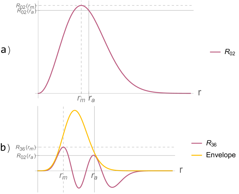
Figure 15: The $R_{nl}(r)$ function as in equation (9)) for the harmonic oscillator in two dimensions, with the values $n=0$, $l=2$ for a) and $n=3$, $l=6$ for b). These square-integrable functions have no divergences in their domain, with a very pronounced decline within a Gaussian envelope. The matrix elements of radius $r$ tend to decrease and their value is less than the most probable radius $r$, showing how the integration of products of these functions will give smaller results as the quantum numbers $n,l$ and $n_{0},l_{0}$ are further apart.

$$\begin{split}R_{nl}(r)=\frac{1}{a}R_{nl}\left(\frac{r}{a}\right),\end{split}$$ (75)

It was shown that, by implementing the harmonic oscillator model to the molecule, the characteristic radius $a$ was determined by the frequency of oscillation. The constant $a$ helps to distinguish the cases $r^{\prime}>a$, $a>r^{\prime}$. From the variable integration limits in (LABEL:Moshinsky_function_variable_limits) and their definition in (28) we infer that a small correction $r^{\prime}>0$ can be imposed with the condition $r^{\prime}\lesssim L$, which in turn is met when $a\lesssim L$ is satisfied. Thus, our truncation of the series (33) is justified regarding the molecular radius. We must also give a criterion for the limits that the energy can have in terms of the incident wavelength. For diffraction phenomena we have the following:

$$\frac{\lambda}{L}\lesssim 1.\\$$ (76)

By focusing on the initial state of energy $E$ and recalling (15), we see that the propagator (16) has unbounded terms in the limit of short wavelengths replaced in (33):

$$\frac{\lambda}{\sqrt{X^{2}+Z^{2}}}<<1,$$ (77)

and large values for $Z$ compared to $X$:

$$\frac{X}{Z}<<1,$$ (78)

but we note how these limits are equivalent to (18) and (19) respectively, thus we can take the approximation (LABEL:propagator_graphics_paraxial). We can directly determine the scale of the successive terms in (33) if we write the elements in the series that contain dimensions:

$$\frac{1}{\sqrt{\lambda Z}}(r^{\prime k})\left[\left(\frac{\partial}{\partial X}\right)^{k-1}e^{i\pi X^{2}/\lambda Z}\right]\left(\frac{\partial X}{\partial r^{\prime}}\right)^{k}.$$

We rescale $r^{\prime}=au$ where $u$ is dimensionless, and we define $\zeta=X/\sqrt{\lambda Z}$ to finally have:

$$(u^{k})\left[\left(\frac{\partial}{\partial\zeta}\right)^{k-1}e^{i\pi\zeta^{2}}\right]\left(\frac{\partial\zeta}{\partial u}\right)^{k},$$

which means that the magnitude of energy enters in $\zeta<1$ for a valid approximation. The conditions (77) and (78) are true even for small $X$, which allows to define a condition that satisfies both:

$$\frac{\lambda}{Z}<<1.$$ (79)

Appendix B Matrix elements of the molecular radius

Here we evaluate (42):

$$f_{ll_{0}}(m_{1},m_{2})=\int_{0}^{2\pi}d\theta^{\prime}e^{-il\theta^{\prime}}e^{il_{0}\theta^{\prime}}S_{-}(m_{1},m_{2},\theta^{\prime}),$$

and according to (28), we know that the function $S_{-}(m_{1},m_{2},\theta^{\prime})$ depends on $\text{cos}(\theta^{\prime})$ in such way, that it is always positive. This allows to rewrite the expression above as:

$$\begin{split}f_{ll_{0}}(m_{1},m_{2})&=a\int_{-\pi/2}^{\pi/2}d\theta^{\prime}e^{i(l-l_{0})\theta^{\prime}}\text{cos}\theta^{\prime}\\ &+b\int_{\pi/2}^{3\pi/2}d\theta^{\prime}e^{i(l-l_{0})\theta^{\prime}}\text{cos}\theta^{\prime},\\ \end{split}$$ (80)

now we evaluate

$$\int d\theta^{\prime}e^{i(l-l_{0})\theta^{\prime}}\text{cos}\theta^{\prime},\\$$

in the following manner

$$\begin{split}\int d\theta^{\prime}e^{i(l-l_{0})\theta^{\prime}}\left(\frac{e^{i\theta^{\prime}}+e^{-i\theta^{\prime}}}{2}\right)=\\ \frac{1}{2}\int d\theta^{\prime}e^{i(l-l_{0}+1)\theta^{\prime}}+\frac{1}{2}\int d\theta^{\prime}e^{i(l-l_{0}-1)\theta^{\prime}},\\ \end{split}$$

which leaves us with

$$\int d\theta^{\prime}e^{i(l-l_{0})\theta^{\prime}}\text{cos}\theta^{\prime}=\frac{1}{2}\left(\frac{e^{i(l-l_{0}+1)\theta^{\prime}}}{i(l-l_{0}+1)}+\frac{e^{i(l-l_{0}-1)\theta^{\prime}}}{i(l-l_{0}-1)}\right),$$ (81)

and we now substitute in (80):

$$\begin{split}f_{ll_{0}}(m_{1},m_{2})&=\left(\frac{a-b}{2}\right)\left(\frac{e^{i(l-l_{0})\frac{\pi}{2}}}{l-l_{0}+1}+\frac{e^{-i(l-l_{0})\frac{\pi}{2}}}{l-l_{0}+1}\right)\\ &-\left(\frac{a-b}{2}\right)\left(\frac{e^{i(l-l_{0})\frac{\pi}{2}}}{l-l_{0}-1}+\frac{e^{-i(l-l_{0})\frac{\pi}{2}}}{l-l_{0}-1}\right)\\ &=\left(a-b\right)\left(\frac{\text{cos}[(l-l_{0})\frac{\pi}{2}]}{l-l_{0}+1}-\frac{\text{cos}[(l-l_{0})\frac{\pi}{2}]}{l-l_{0}-1}\right)\\ &=\left(a-b\right)\text{cos}\left[(l-l_{0})\frac{\pi}{2}\right]\frac{2}{1-(l-l_{0})^{2}},\end{split}$$ (82)

where $e^{i\frac{3\pi}{2}}=e^{-i\frac{\pi}{2}}$ was used; now, according to the definition in (44):

$$f_{ll_{0}}(m_{1},m_{2})=\left(a-b\right)\zeta_{l-l_{0}}\frac{2}{1-(l-l_{0})^{2}},$$ (83)

our final task left is to evaluate $(a-b)$; $a$ and $b$ can be known from (28):

$$a=\frac{m_{2}}{M}\;\;\;\;\;\;b=-\frac{m_{1}}{M},$$

and implies

$$a-b=1.$$

Therefore, the dependence on $m_{1}$ and $m_{2}$ vanishes and we obtain (44). The process for obtaining (43) is similar and we obtain an analogous result to (83):

$$g_{ll_{0}}(m_{1},m_{2})=\left(c-d\right)\zeta_{l-l_{0}}\frac{2}{1-(l-l_{0})^{2}}.$$

By looking again at (28) (but working this time with $S_{+}(\theta^{\prime},m_{1},m_{2})$) we obtain:

$$\begin{gathered}c=-\frac{m_{1}}{M}\;\;\;\;\;\;d=\frac{m_{2}}{M}\\ c-d=-1,\end{gathered}$$

and finally

$$g_{ll_{0}}=-f_{ll_{0}}.$$

References

- (1) I. Bloch, J. Dalibard, and W. Zwerger. Many-body physics with ultracold gases. Rev. Mod. Phys. 80 3 (2008), 885–964. doi:10.1103/RevModPhys.80.885.
- (2) W. Campbell. Atomic envoy enables molecular control. Nature 545 (2017), 164.
- (3) B. Brezger, M. Arndt, and A. Zeilinger. Concepts for near-field interferometers with large molecules. Journal of Optics B: Quantum and Semiclassical Optics 5 2 (2003), S82–S89. doi:10.1088/1464-4266/5/2/362.
- (4) S. Truppe, M. Hambach, S. M. Skoff, N. E. Bulleid, J. S. Bumby, R. J. Hendricks, E. A. Hinds, B. E. Sauer, and M. R. Tarbutt. A buffer gas beam source for short, intense and slow molecular pulses. Journal of Modern Optics 65 5-6 (2018), 648–656. doi:10.1080/09500340.2017.1384516.
- (5) N. Dörre, J. Rodewald, P. Geyer, B. von Issendorff, P. Haslinger, and M. Arndt. Photofragmentation Beam Splitters for Matter-Wave Interferometry. Phys. Rev. Lett. 113 23 (2014), 233001. doi:10.1103/PhysRevLett.113.233001.
- (6) M. S. Chapman, C. R. Ekstrom, T. D. Hammond, R. A. Rubenstein, J. Schmiedmayer, S. Wehinger, and D. E. Pritchard. Optics and Interferometry with Na 2 Molecules. Phys. Rev. Lett. 74 24 (1995), 4783–4786. doi:10.1103/PhysRevLett.74.4783.
- (7) B. Brezger, L. Hackermüller, S. Uttenthaler, J. Petschinka, M. Arndt, and A. Zeilinger. Matter-Wave Interferometer for Large Molecules. Phys. Rev. Lett. 88 10 (2002), 100404. doi:10.1103/PhysRevLett.88.100404.
- (8) P. Haslinger, N. Dörre, P. Geyer, J. Rodewald, S. Nimmrichter, and M. Arndt. A universal matter-wave interferometer with optical ionization gratings in the time domain. Nature Physics 9 (2013), 144.
- (9) K. Hornberger, S. Gerlich, P. Haslinger, S. Nimmrichter, and M. Arndt. Colloquium: Quantum interference of clusters and molecules. Rev. Mod. Phys. 84 1 (2012), 157–173. doi:10.1103/RevModPhys.84.157.
- (10) W. B. Case, E. Sadurní, and W. P. Schleich. A diffractive mechanism of focusing. Opt. Express 20 25 (2012), 27253. doi:10.1364/OE.20.027253.
- (11) S. Gerlich, L. Hackermüller, K. Hornberger, A. Stibor, H. Ulbricht, M. Gring, F. Goldfarb, T. Savas, M. Müri, M. Mayor, and M. Arndt. A Kapitza–Dirac–Talbot–Lau interferometer for highly polarizable molecules. Nature Physics 3 10 (2007), 711–715. doi:10.1038/nphys701.
- (12) W. Nawrocki. Introduction to Quantum Metrology: The Revised SI System and Quantum Standards. Springer, Cham (2019). OCLC: 1121435806.
- (13) G. Summy. Molecular Interferometry Makes a New Break. Physics 7 (2014), 122. doi:10.1103/Physics.7.122.
- (14) B. W. Shore, P. Dömötör, E. Sadurní, G. Süssmann, and W. P. Schleich. Scattering of a particle with internal structure from a single slit. New J. Phys. 17 1 (2015), 013046. doi:10.1088/1367-2630/17/1/013046.
- (15) P. Dömötör, P. Földi, M. G. Benedict, B. W. Shore, and W. P. Schleich. Scattering of a particle with internal structure from a single slit: Exact numerical solutions. New J. Phys. 17 2 (2015), 023044. doi:10.1088/1367-2630/17/2/023044.
- (16) P. Dömötör, and M. G. Benedict. Scattering of a classical rotating object by a screen with a slit. Phys. Scr. 94 2 (2019), 024002. doi:10.1088/1402-4896/aaf142.
- (17) D. Condado, J. L. Díaz-Cruz, A. Rosado, and E. Sadurní. Diffraction of particles in free fall. Phys. Rev. A 98 4 (2018), 043618. doi:10.1103/PhysRevA.98.043618.
- (18) J. D. Jackson. Classical Electrodynamics. Wiley, New York, 3rd ed edition (1999).
- (19) C. Grosche and F. Steiner. Handbook of Feynman Path Integrals. Number 145 in Springer Tracts in Modern Physics. Springer Verlag, New York (1998).
- (20) E. Sadurní. Exact propagators on the lattice with applications to diffractive effects. J. Phys. A: Math. Theor. 45 46 (2012), 465302. doi:10.1088/1751-8113/45/46/465302.
- (21) C.-w. Chou, C. Kurz, D. B. Hume, P. N. Plessow, D. R. Leibrandt, and D. Leibfried. Preparation and coherent manipulation of pure quantum states of a single molecular ion. Nature 545 7653 (2017), 203–207. doi:10.1038/nature22338.
- (22) M. Moshinsky. Diffraction in Time. Phys. Rev. 88 3 (1952), 625–631. doi:10.1103/PhysRev.88.625.
- (23) V. N. Faddeeva and N. M. Terent’ev. Tables of Values of the Function for Complex Argument. Pergamon Press, Oxford (1961).
- (24) S. Cordero and G. García-Calderón. Diffraction in time for tunneling invisibility in quantum systems. Phys. Rev. A 88 5 (2013), 052118. doi:10.1103/PhysRevA.88.052118.
- (25) M. J. J. Vrakking, D. M. Villeneuve, and A. Stolow. Observation of fractional revivals of a molecular wave packet. Phys. Rev. A 54 1 (1996), R37–R40. doi:10.1103/PhysRevA.54.R37.
- (26) A. Lee, T. Kalotas, and N. Adams. Modified Morse Potential for Diatomic Molecules. Journal of Molecular Spectroscopy 191 1 (1998), 137–141. doi:10.1006/jmsp.1998.7629.
- (27) B. W. Shore. Comparison of matrix methods applied to the radial Schrödinger eigenvalue equation: The Morse potential. The Journal of Chemical Physics 59 12 (1973), 6450–6463. doi:10.1063/1.1680025.
- (28) M. Berrondo and A. Palma. The algebraic approach to the Morse oscillator. Journal of Physics A: Mathematical and General 13 3 (1980), 773–780. doi:10.1088/0305-4470/13/3/010.
- (29) L. Infeld and T. E. Hull. The Factorization Method. Rev. Mod. Phys. 23 1 (1951), 21–68. doi:10.1103/RevModPhys.23.21.
- (30) E. Karimi, R. W. Boyd, P. de la Hoz, H. de Guise, J. eháek, Z. Hradil, A. Aiello, G. Leuchs, and L. L. Sánchez-Soto. Radial quantum number of Laguerre-Gauss modes. Phys. Rev. A 89 6 (2014), 063813. doi:10.1103/PhysRevA.89.063813.
- (31) M. Abramowitz and I. A. Stegun, editors. Handbook of Mathematical Functions: With Formulas, Graphs, and Mathematical Tables. Dover Books on Mathematics. Dover Publ, New York, 9. dover print.; [nachdr. der ausg. von 1972] edition (2013). OCLC: 935935300.
- (32) K. P. Huber and G. Herzberg. Molecular Spectra and Molecular Structure - IV. Constants of Diatomic Molecules. Springer-Verlag New York, New York (2013). OCLC: 922651164.
- (33) H. Talbot. LXXVI. Facts relating to optical science. No. IV. The London, Edinburgh, and Dublin Philosophical Magazine and Journal of Science 9 56 (1836), 401–407. doi:10.1080/14786443608649032.
- (34) M. Berry, I. Marzoli, and W. Schleich. Quantum carpets, carpets of light. Phys. World 14 6 (2001), 39–46. doi:10.1088/2058-7058/14/6/30.
- (35) W. B. Case, M. Tomandl, S. Deachapunya, and M. Arndt. Realization of optical carpets in the Talbot and Talbot-Lau configurations. Opt. Express 17 23 (2009), 20966. doi:10.1364/OE.17.020966.