Non-Parametric Graph Learning for Bayesian Graph Neural Networks

Abstract

Graphs are ubiquitous in modelling relational structures. Recent endeavours in machine learning for graph structured data have led to many architectures and learning algorithms. However, the graph used by these algorithms is often constructed based on inaccurate modelling assumptions and/or noisy data. As a result, it fails to represent the true relationships between nodes. A Bayesian framework which targets posterior inference of the graph by considering it as a random quantity can be beneficial. In this paper, we propose a novel non-parametric graph model for constructing the posterior distribution of graph adjacency matrices. The proposed model is flexible in the sense that it can effectively take into account the output of graph based learning algorithms that target specific tasks. In addition, model inference scales well to large graphs. We demonstrate the advantages of this model in three different problem settings: node classification, link prediction and recommendation.

1 INTRODUCTION

Growing interest in inference tasks involving networks has prompted the need for learning architectures adapted to graph-structured data. As a result, numerous models have been proposed for addressing various graph based learning tasks such as classification, link prediction, and recommendation. These approaches process the observed graph as if it depicts the true relationship among the nodes. In practice, the observed graphs are formed based on imperfect observations and incorrect modelling assumptions. Spurious edges might be formed and important links might be deleted. The vast majority of existing algorithms cannot take the uncertainty of the graph structure into account during training as there is no mechanism for removing spurious edges and/or adding informative edges in the observed graph.

Several algorithms that do address this uncertainty by incorporating a graph learning component have been proposed recently [Zhang et al., 2019, Ma et al., 2019, Tiao et al., 2019, Jiang et al., 2019]. These methods have limitations, either involving parametric graph models that restrict their applicability or being focused on the task of node classification.

In this work, we propose a non-parametric graph inference technique which is incorporated in a Bayesian framework to tackle node and/or edge level learning tasks. Our approach has the following key benefits. First, it generalizes the applicability of the Bayesian techniques outside the realm of parametric modelling. Second, flexible, task specific graph learning can be achieved; this makes effective use of the outputs of existing graph-learning techniques to improve upon them. Third, the graph learning procedure scales well to large graphs, in contrast to the increased difficulty of parametric approaches.

We conduct extensive experiments to demonstrate the usefulness of our model for three different graph related tasks. In a node classification setting we observed increased accuracy for settings where the amount of labeled data is very limited. For the setting of unsupervised learning, we show that incorporating a graph learning step when performing variational modelling of the graph structure with auto-encoder models leads to better link prediction. Finally, a Bayesian approach based on our proposed model improves recall for existing state-of-the-art graph-based recommender system architectures.

2 RELATED WORK

Topology uncertainty in graph neural networks:

The most closely related work to our proposed approach is a group of recent techniques that jointly perform inference of the graph while addressing a learning task such as node classification. The recently proposed Bayesian GCN [Zhang et al., 2019] provides a general, principled framework to deal with the issue of uncertainty on graphs. Similar ideas are considered in [Ma et al., 2019], where variational inference is used to learn the graph structure. This formulation allows consideration of additional data such as features and labels when performing graph inference, but the technique is still tied to a parametric model. In [Tiao et al., 2019], the authors take a non-parametric approach, but their probabilistic formulation is focused on improving only very noisy graphs. In [Jiang et al., 2019], simultaneous optimization of the graph structure along with the learning task is considered. In all of these works, only the node classification task has been explored. Our methodology extends the applicability of these methods by combining the Bayesian framework with a more flexible non-parametric graph model.

Graph learning:

Multiple algorithms have been proposed that focus exclusively on learning graph connectivity based on observed data [Dong et al., 2016, Kalofolias, 2016]. These works differ from ours in that the end goal is topology inference. These algorithms typically appeal to a smoothness criterion for the graph. Although these methods provide useful graphs, they have $\mathcal{O}(N^{2})$ complexity. As a result, many do not scale well to large graphs. Approximate nearest neighbour (A-NN) graph learning [Malkov and Yashunin, 2020] has $\mathcal{O}(N\log N)$ complexity, which is more suitable for large scale applications, but the learned graph generally has poor quality compared to the k-NN graph. A more recent method in [Kalofolias and Perraudin, 2019] introduces an approximate graph learning algorithm which provides an efficient trade off between runtime and the quality of the solution. We build on this method for our inference procedure, but our graph model is tailored to the specific learning task we address.

Deep learning based graph generative models:

There is a large body of existing work for deep learning based graph generative models. In [Li et al., 2018, Simonovsky and Komodakis, 2018, You et al., 2018, Liao et al., 2019, Liu et al., 2019] various algorithms for graph generation using VAEs, RNNs, and normalizing flow are developed. These approaches are evaluated based on the likelihood of sampled graphs and comparing graph characteristics. Moreover these algorithms do not preserve node identities, so sampled (inferred) graphs cannot be directly used for node or edge level inference. Generative adversarial networks (GANs) based approaches [Wang et al., 2017, Bojchevski et al., 2018] are more successful in sampling graphs similar to the observed one. However, these models have prohibitively high computational complexity and their performance is heavily dependent on hyperparameter tuning.

Node classification:

A central learning task on graphs is semi-supervised node classification. In general, the most common approach is to incorporate graph filters within deep learning algorithms. Early works [Duvenaud et al., 2015, Defferrard et al., 2016] based their models on theory from the graph signal processing community. This approach led to more sophisticated graph convolution architectures [Kipf and Welling, 2017, Veličković et al., 2018, Hamilton et al., 2017]. More recent models include [Zhuang and Ma, 2018, Wijesinghe and Wang, 2019]. In [Tian et al., 2019], a learnable graph kernel based on a data-driven similarity metric is considered for node classification. Our graph learning framework can be combined with these algorithms to augment performance, particularly when there is a very limited amount of labelled data.

Link prediction:

Several algorithms based on autoencoders have been shown to perform extremely well for the link prediction task [Kipf and Welling, 2016, Pan et al., 2018, Grover et al., 2019, Mehta et al., 2019]. These techniques learn node embeddings in a (variational) autoencoder framework and model the probability of the existence of an edge based on the closeness of the embeddings. We show how our method can be combined with these strategies to deliver a small but consistent improvement for the link prediction task.

Recommender systems:

Recommender systems have become a key factor to meet users’ diverse and personalized needs for online consumption platforms. The most common approach is collaborative filtering (CF). Recent works have incorporated graphs and GNNs to better model the user-item interactions [van den Berg et al., 2018, Ying et al., 2018, Wang et al., 2019, Sun et al., 2019, Monti et al., 2017, Zheng et al., 2018].

Although the GNN-based recommendation models have achieved impressive performance, existing methods regard the provided user–item interaction records as ground truth. In many practical settings, the user-item interaction graph has spurious edges due to noisy information; on the other hand, some potential user-item positive interactions are missing because the item is never presented to the user. This is falsely indicated as a negative interaction. Thus, it is important to capture the uncertainty in the observed user-item interaction graph. In the following methodology section, we elaborate on how our graph learning approach can alleviate this problem.

3 METHODOLOGY

3.1 NON-PARAMETRIC GRAPH LEARNING

In many learning tasks, often an observed graph $\mathcal{G}_{obs}$ provides additional structure to the given data $\mathcal{D}$. The data $\mathcal{D}$ can include feature vectors, labels, and other information, depending on the task at hand. If $\mathcal{G}_{obs}$ is not readily available, it is often built from the data $\mathcal{D}$ and possibly other side-information. In many cases, $\mathcal{G}_{obs}$ does not represent the true relationship of the nodes as it is often formed using inaccurate modelling assumptions and/or is constructed from noisy data. In several recent works [Zhang et al., 2019, Ma et al., 2019, Tiao et al., 2019], it has been shown that building a posterior model for the ‘true’ graph $\mathcal{G}$ and incorporating it in the learning task is beneficial.

We propose a non-parametric generative model for the adjacency matrix $\mathbf{A}_{\mathcal{G}}$ of the random undirected graph $\mathcal{G}$. $\mathbf{A}_{\mathcal{G}}$ is assumed to be a symmetric matrix with non-negative entries. We emphasize that our model retains the identities of the nodes and disallows permutations of nodes (permutations of adjacency matrices are not equivalent graphs when node identities are preserved). This characteristic is essential for its use in node and edge level inference tasks. We define the prior distribution for $\mathcal{G}$ as

$$p(\mathcal{G})\propto\begin{dcases}e^{\left(\alpha\mathbf{1}^{\top}\log(\mathbf{A}_{\mathcal{G}}\mathbf{1})-\beta\|\mathbf{A}_{\mathcal{G}}\|_{F}^{2}\right)}\,,&\text{ if }\mathbf{A}_{\mathcal{G}}\geq\mathbf{0}\\ &\text{\phantom{ if }}\mathbf{A}_{\mathcal{G}}=\mathbf{A}_{\mathcal{G}}^{\top}\\ 0\,,&\text{otherwise}\,.\end{dcases}$$ (1)

The first term in the log prior is a logarithmic barrier on the degree of the nodes which prevents any isolated node in $\mathcal{G}$. The second term is a regularizer based on the Frobenius norm which encourages low weights for the links. $\alpha$ and $\beta$ are hyperparameters which control the scale and sparsity of $A_{\mathcal{G}}$. In our model, the joint likelihood of $\mathcal{G}_{obs}$ and $\mathcal{D}$ conditioned on $\mathcal{G}$ is:

$$p(\mathcal{G}_{obs},\mathcal{D}|\mathcal{G})\propto\exp{(-\|\mathbf{A}_{\mathcal{G}}\circ\mathbf{D}(\mathcal{G}_{obs},\mathcal{D})\|_{1,1})}\,,$$ (2)

where $\mathbf{D}(\mathcal{G}_{obs},\mathcal{D})\geq\mathbf{0}$ is a symmetric pairwise distance matrix which encodes the dissimilarity between the nodes. The symbol $\circ$ denotes the Hadamard product and $\|\cdot\|_{1,1}$ denotes the elementwise $\ell_{1}$ norm. The likelihood encourages higher edge weights for the node pairs with lower pairwise distances and vice versa.

Bayesian inference of the graph $\mathcal{G}$ involves sampling from its posterior distribution. The space is high dimensional ($\mathcal{O}(N^{2})$, where $N$ is the number of the nodes). Designing a suitable sampling scheme (e.g., Markov Chain Monte Carlo) in such a high dimensional space is extremely challenging and computationally demanding for large graphs. Instead we pursue maximum a posteriori estimation, which is equivalent to approximating the posterior by a point mass at the mode [MacKay, 1996]. We solve the following optimization problem:

$$\widehat{\mathcal{G}} =\operatorname*{arg\,max}_{\mathcal{G}}p(\mathcal{G}|\mathcal{G}_{obs},\mathcal{D})\,,$$ (3)

which is equivalent to learning an $N\!\times\!N$ symmetric adjacency matrix of $\widehat{\mathcal{G}}$.

$$\mathbf{A}_{\widehat{\mathcal{G}}} =\operatorname*{arg\,min}_{\begin{subarray}{c}\mathbf{A}_{\mathcal{G}}\in\mathbf{R_{+}}^{N\times N},\\ \mathbf{A}_{\mathcal{G}}=\mathbf{A}_{\mathcal{G}}^{\top}\end{subarray}}\begin{aligned} &\|\mathbf{A}_{\mathcal{G}}\circ\mathbf{D}\|_{1,1}-\alpha\mathbf{1}^{\top}\log(\mathbf{A}_{\mathcal{G}}\mathbf{1})\\ &\quad\quad\quad\quad\quad\quad\quad+\beta\|\mathbf{A}_{\mathcal{G}}\|_{F}^{2}\,.\end{aligned}$$ (4)

The optimization problem in (4) has been studied in the context of graph learning from smooth signals. [Kalofolias, 2016] adopts a primal-dual optimization technique to solve this problem. However the complexity of this approach scales as $\mathcal{O}(N^{2})$, which can be prohibitive for large graphs. In this paper, we employ the scalable, approximate algorithm in  [Kalofolias and Perraudin, 2019], which has several advantages as follows. First, it can use existing approximate nearest neighbour techniques, as in [Malkov and Yashunin, 2020], to reduce the dimensionality of the optimization problem. Second, the graph learning has a computational complexity of $\mathcal{O}(N\log N)$ (the same as approximate nearest neighbour algorithms), while the quality of the learned graph is comparable to the state-of-the-art. Third, if we are not concerned about the scale of the learned graph (which is typical in many learning tasks we consider, since a normalized version of the adjacency or Laplacian matrix is used), the approximate algorithm allows us to effectively use only one hyperparameter instead of $\alpha$ and $\beta$ to control the sparsity of the solution and provides a useful heuristic for automatically selecting a suitable value based on the desired edge density of the solution.

In our work, we use this approximate algorithm for inference of the graph $\mathcal{G}$, which is subsequently used in various learning tasks. Since, we have freedom in choosing a functional form for $\textbf{D}(\cdot,\cdot)$, we can design suitable distance metrics in a task specific manner. This flexibility allows us to incorporate the graph learning step in diverse tasks. In the next three subsections, we present how the graph learning step can be applied to develop Bayesian algorithms for node classification, link prediction and recommendation systems.

3.2 NODE CLASSIFICATION

Problem Statement:

We consider a semi-supervised node classification problem for the nodes in $\mathcal{G}_{obs}$. In this setting we also have access to the node attributes $\mathbf{X}$ and the labels in the training set $\mathbf{Y_{\mathcal{L}}}$. So, $\mathcal{D}=(\mathbf{X},\mathbf{Y_{\mathcal{L}}})$. The task is to predict the labels of the remaining nodes $\mathbf{Y_{\overline{\mathcal{L}}}}$, where $\overline{\mathcal{L}}=\mathcal{V}\setminus\mathcal{L}$.

Bayesian GCN – non-parametric model:

[Zhang et al., 2019] derive a Bayesian learning methodology for GCNs by building a posterior model for $\mathcal{G}$. Their approach assumes that $\mathcal{G}_{obs}$ is sampled from a parametric graph model. The graph model parameters are marginalized to target inference of the graph posterior $p(\mathcal{G}|\mathcal{G}_{obs})$. Although this approach is effective, it has several drawbacks. The methodology lacks flexibility since a particular parametric model might not fit different types of graph. Bayesian inference of the model parameters is often challenging for large graphs. Finally, parametric modelling of graphs cannot use the information provided by the node features $\mathbf{X}$ and training labels $\mathbf{Y_{\mathcal{L}}}$ for inference of $\mathcal{G}$. Here, we propose to incorporate a non-parametric model for inference of $\mathcal{G}$ in the BGCN framework. We aim to compute the marginal posterior probability of the node labels, which is obtained via marginalization with respect to the graph $\mathcal{G}$ and GCN weights $\mathbf{W}$:

$$p(\mathbf{Z}|\mathbf{Y_{\mathcal{L}}},\mathbf{X},\mathcal{G}_{obs}) =\int p(\mathbf{Z}|\mathbf{W},\mathcal{G}_{obs},\mathbf{X})p(\mathbf{W}|\mathbf{Y_{\mathcal{L}}},\mathbf{X},\mathcal{G})\,$$

$$\qquad p(\mathcal{G}|\mathcal{G}_{obs},\mathbf{X},\mathbf{Y_{\mathcal{L}}})\,d\mathbf{W}\,d\mathcal{G}\,.$$ (5)

The categorical distribution of the node labels $p(\mathbf{Z}|\mathbf{Y_{\mathcal{L}}},\mathbf{X},\mathcal{G}_{obs})$ is modelled by applying a softmax function to the output of the last layer of the GCN. The integral in (5) cannot be computed in a closed form, so we employ Monte Carlo to approximate it as follows:

$$p(\mathbf{Z}|\mathbf{Y_{\mathcal{L}}},\mathbf{X},\mathcal{G}_{obs})\approx\dfrac{1}{S}\sum_{s=1}^{S}p(\mathbf{Z}|\mathbf{W}_{s},\mathcal{G}_{obs},\mathbf{X})\,.$$ (6)

Here, we learn the maximum a posteriori (MAP) estimate $\widehat{\mathcal{G}}=\displaystyle{\operatorname*{arg\,max}_{\mathcal{G}}}\hskip 5.0ptp(\mathcal{G}|\mathcal{G}_{obs},\mathbf{X},\mathbf{Y_{\mathcal{L}}})$ and subsequently sample $S$ weight matrices $\mathbf{W}_{s}$ from $p(\mathbf{W}|\mathbf{Y_{\mathcal{L}}},\mathbf{X},\widehat{\mathcal{G}})$ by training a Bayesian GCN using the graph $\widehat{\mathcal{G}}$.

In order to perform the graph learning step, we need to define a pairwise distance matrix $\mathbf{D}$. For this application, we propose to combine the output of a node embedding algorithm and a base classifier to form $\mathbf{D}$:

$$\mathbf{D}(\mathbf{X},\mathbf{Y_{\mathcal{L}}},\mathcal{G}_{obs})=\mathbf{D}_{1}(\mathbf{X},\mathcal{G}_{obs})+\delta\mathbf{D}_{2}(\mathbf{X},\mathbf{Y_{\mathcal{L}}},\mathcal{G}_{obs})\,.$$ (7)

Here $\delta$ is a hyperparameter which controls the importance of $\mathbf{D}_{2}$ relative to $\mathbf{D}_{1}$. The $(i,j)$’th entries of $\mathbf{D}_{1}$ and $\mathbf{D}_{2}$ are defined as follows:

$$D_{1,ij}(\mathbf{X},\mathcal{G}_{obs}) =\|\bm{z}_{i}-\bm{z}_{j}\|^{2}\,,$$ (8)

$$D_{2,ij}(\mathbf{X},\mathbf{Y_{\mathcal{L}}},\mathcal{G}_{obs}) =\frac{1}{|\mathcal{N}_{i}||\mathcal{N}_{j}|}\displaystyle{\sum_{k\in\mathcal{N}_{i}}\sum_{l\in\mathcal{N}_{j}}}\mathbb{1}_{(\hat{c}_{k}\neq\hat{c}_{l})}\,.$$ (9)

Here, $\bm{z}_{i}$ is any suitable embedding of node $i$ and $\hat{c}_{i}$ is the predicted label at node $i$ obtained from the base classification algorithm. $\mathbf{D}_{1}$ measures pairwise dissimilarity in terms of the observed topology and features and $\mathbf{D}_{2}$ summarizes the discrepancy of the node labels in the neighbourhood. For the experiments, we choose the Variational Graph Auto-Encoder (VGAE) algorithm [Kipf and Welling, 2016] as the node embedding method to obtain the $\bm{z}_{i}$ vectors and use the GCN proposed by [Kipf and Welling, 2017] as the base classifier to obtain the $\hat{c}_{i}$ values. The neighbourhood of the $i$-th node is defined as:

$$\mathcal{N}_{i}=\{j|(i,j)\in\mathcal{E}_{\mathcal{G}_{obs}}\}\cup\{i\}\,.$$

Here, $\mathcal{E}_{\mathcal{G}_{obs}}$ is the set of edges in $\mathcal{G}_{obs}$. With the regard to the choice of the hyperparameter $\delta$, we observe that

$$\delta=\dfrac{\displaystyle{\max_{i,j}}\hskip 5.0ptD_{1,ij}}{\displaystyle{\max_{i,j}}\hskip 5.0ptD_{2,ij}}$$

works well in our experiments, although it can be tuned via cross-validation if a validation set is available.

For the inference of GCN weights $\mathbf{W}$, many existing algorithms such as expectation propagation [Hernández-Lobato and Adams, 2015], variational inference [Gal and Ghahramani, 2016, Sun et al., 2017], and Markov Chain Monte Carlo methods [Neal, 1992, Li et al., 2016] can be employed. As in [Zhang et al., 2019], we train a GCN on the inferred graph $\widehat{\mathcal{G}}$ and use Monte Carlo dropout [Gal and Ghahramani, 2016]. This is equivalent to sampling $\mathbf{W}_{s}$ from a particular variational approximation of $p(\mathbf{W}|\mathbf{Y_{\mathcal{L}}},\mathbf{X},\widehat{\mathcal{G}})$. The resulting algorithm is provided in the supplementary material.

3.3 LINK PREDICTION

Problem statement:

In this setting, some of the links in $\mathcal{G}_{obs}$ are hidden or unobserved. The task is to predict the unseen links based on the knowledge of the (partially) observed $\mathcal{G}_{obs}$ and the node features $\mathbf{X}$. Thus in this case, the additional data beyond the graph is $\mathcal{D}=\mathbf{X}$.

Background:

In existing works, the link prediction problem is addressed by building deep learning based generative models for graphs. In particular, various architectures of graph variational auto-encoders [Kipf and Welling, 2016, Grover et al., 2019, Mehta et al., 2019] aim to learn the posterior distribution of the node embedding $\bm{Z}$ conditioned on the observed graph $\mathcal{G}_{obs}$ and the node features $\mathbf{X}$. The inference model (encoder) often uses simplifying assumptions (e.g. mean-field approximation over nodes or diagonal covariance structures) for the parametric form of the approximate variational posterior distribution $q(\bm{Z}|\mathcal{G}_{obs},\mathbf{X})$. Deep learning architectures are used to learn the parameters of the model. The decoder is another deep learning model which explains how the graph is generated from the embeddings, i.e., it parameterizes $p(\mathcal{G}_{obs}|\bm{Z},\mathbf{X})$. Typically the probability of a link in these models is dependent on the similarity of the embedding of the two incident nodes. Assuming a suitable prior $p(\bm{Z})$, the encoder and decoder is trained jointly to minimize the KL divergence between $q(\bm{Z}|\mathcal{G}_{obs},\mathbf{X})$ and the true posterior $p(\bm{Z}|\mathcal{G}_{obs},\mathbf{X})$. The learned embeddings are evaluated based on an amortized link prediction task for the unseen portion of the graph.

Proposed methodology – Bayesian VGAE:

We consider a Bayesian formulation, where we conduct Bayesian inference of the graph $\mathcal{G}$ in the encoder. Let us introduce a function $\mathcal{J}(\mathcal{G},\mathcal{G}_{obs})$ that returns a graph such that the unobserved entries of the adjacency matrix of $\mathcal{G}_{obs}$ are replaced by the corresponding entries of $\mathcal{G}$. We then model the inference distribution as follows:

$$q(\bm{Z}|\mathcal{G}_{obs},\mathbf{X}) =\int q(\bm{Z}|\mathcal{J}(\mathcal{G},\mathcal{G}_{obs}),\mathbf{X})p(\mathcal{G}|\mathcal{G}_{obs},\mathbf{X})d\mathcal{G}\,,$$

$$\approx q(\bm{Z}|\mathcal{J}(\widehat{\mathcal{G}},\mathcal{G}_{obs}),\mathbf{X})\,,$$

where $\widehat{\mathcal{G}}=\displaystyle{\operatorname*{arg\,max}_{\mathcal{G}}}\hskip 5.0ptp(\mathcal{G}|\mathcal{G}_{obs},\mathbf{X})$ is the MAP estimate from the non-parametric model. The intuitive idea behind this modeling is that if the non-parametric inference provides a reasonable approximation of the unobserved adjacency matrix entries, then an auto encoder trained on a graph that incorporates these approximate entries should learn better embeddings. For the graph learning step, we form the distance matrix $\mathbf{D}$ using the output of an auto-encoder as follows:

$$D_{ij}(\mathbf{X},\mathcal{G}_{obs}) =\|\mathbb{E}_{q}[\bm{z}_{i}]-\mathbb{E}_{q}[\bm{z}_{j}]\|^{2}\,.$$ (10)

The resulting algorithm is summarized in the supplementary material.

3.4 RECOMMENDATION SYSTEMS

Problem statement:

In this section we address a personalized item recommendation task based on historical interaction data. We denote the set of users and items by $\mathcal{U}$ and $\mathcal{I}$ respectively. The interaction between any user $u\in\mathcal{U}$ and item $i\in\mathcal{I}$ is encoded as a link in a bipartite graph $\mathcal{G}_{obs}$. The task is to infer the unobserved interactions (and to use these as predictions of future interactions). Viewed in this light, the recommendation task is a link prediction problem. However, in many cases, predicting a personalized ranking for the items is important [Rendle et al., 2009].

For each user $u$, if there is an observed interaction with item $i$ and an unobserved interaction with item $j$, we write that $i>_{u}j$ in the training set. The introduced relation $i>_{u}j$ implies that user $u$ prefers item $i$ to item $j$. This interaction training data leads to a set of rankings $\{>_{u}\}_{trn}$ for each user $u$ over the training set of triples: $\{(u,i,j):(u,i)\in\mathcal{G}_{obs},(u,j)\notin\mathcal{G}_{obs}\}$. We denote these rankings for all users in $\mathcal{U}$ as $\{>_{\mathcal{U}}\}_{trn}$. This training data is used to learn a model parameterized by $\mathbf{W}$. The generalization capability is tested by ranking, for each user $u$, all $(u,i,j)$ such that both $(u,i)$ and $(u,j)\notin\mathcal{G}_{obs}$. We denote the rankings for a specific user in this test set $\{(u,i,j):(u,i)\notin\mathcal{G}_{obs},(u,j)\notin\mathcal{G}_{obs}\}$ as $\{>_{u}\}_{test}$. The collection of all such rankings for all users is denoted $\{>_{\mathcal{U}}\}_{test}$ In this paper, we propose to incorporate Bayesian inference of graph $\mathcal{G}$ in the Bayesian Personalized Ranking (BPR) loss formulation [Rendle et al., 2009]. A brief review of the BPR loss is provided for completeness.

Background – BPR loss:

Many existing graph based deep learning recommender systems [Sun et al., 2019, Wang et al., 2019, Ying et al., 2018] learn an embedding $e_{u}(\mathbf{W},\mathcal{G}_{obs})$ for user $u$ and $e_{i}(\mathbf{W},\mathcal{G}_{obs})$ for item $i$ and model the probability that user $u$ prefers item $i$ to item $j$ as follows:

$$p(i>_{u}j|\mathcal{G}_{obs},\mathbf{W})=\sigma(e_{u}\bm{\cdot}e_{i}-e_{u}\bm{\cdot}e_{j})\,.$$

Here $\sigma(\cdot)$ is the sigmoid function and $\bm{\cdot}$ is the inner product. Our goal is to compute:

$$p(\{>_{\mathcal{U}}\}_{test}| \{>_{\mathcal{U}}\}_{train},\mathcal{G}_{obs})=\int p(\{>_{\mathcal{U}}\}_{test}|\mathcal{G}_{obs},\mathbf{W})\,$$

$$p(\mathbf{W}|\{>_{\mathcal{U}}\}_{train},\mathcal{G}_{obs})d\mathbf{W}\,,$$ (11)

but this integral is not tractable. In practice, we assume a prior $\mathcal{N}(\mathbf{0},\lambda^{-1}I)$ for $\mathbf{W}$ and model the preferences of different users as independent. We can then consider a MAP estimate of $\mathbf{W}$:

$$\widehat{\mathbf{W}} =\operatorname*{arg\,max}_{\mathbf{W}}p(\mathbf{W}|\{>_{\mathcal{U}}\}_{train},\mathcal{G}_{obs})\,,$$

$$=\operatorname*{arg\,max}_{\mathbf{W}}p(\mathbf{W})p(\{>_{\mathcal{U}}\}_{train},\mathcal{G}_{obs}|\mathbf{W})\,,$$

$$=\operatorname*{arg\,max}_{\mathbf{W}}\bigg{(}-\frac{\lambda}{2}\lvert\lvert\mathbf{W}\rvert\rvert^{2}+\,$$

$$\quad\quad\sum_{(u,i,j)\in\{>_{\mathcal{U}}\}_{trn}}\log\left(\sigma(e_{u}\bm{\cdot}e_{i}-e_{u}\bm{\cdot}\cdot e_{j}\right)\bigg{)}\,.$$

This is equivalent to minimizing the BPR loss, where the positive pool $\{(u,i):(u,i)\in\mathcal{G}_{obs}\}$ and negative pool $\{(u,j):(u,j)\notin\mathcal{G}_{obs}\}$ are created according to $\mathcal{G}_{obs}$. Once the MAP estimate has been obtained, we assess the performance by ranking the test set triples using $\widehat{\mathbf{W}}$.

Non-parametric model – Bayesian graph recommender system:

In the Bayesian setting, ranking is conducted by considering an expectation with respect to the posterior distribution of the graph $\mathcal{G}$ from the non-parametric model $p(\mathcal{G}|\mathcal{G}_{obs},\{>_{\mathcal{U}}\}_{train})$. We need to evaluate the posterior probability of ranking in the test set. Let us introduce the graph $\widetilde{G}=\mathcal{J}_{r}(\mathcal{G},\mathcal{G}_{obs})$, which is obtained via a function $\mathcal{J}_{r}$ that combines the information in $\mathcal{G}$ and $\mathcal{G}_{obs}$. We specify the function $\mathcal{J}_{r}$ that we employ in our methodology more precisely below. We can then write the posterior probability of the ranking of the test set as follows:

$$p(\{>_{\mathcal{U}}\}_{test}|\{>_{\mathcal{U}}\}_{train},\mathcal{G}_{obs})=\int p(\{>_{\mathcal{U}}\}_{test}|\mathcal{G}_{obs},\mathbf{W})\,$$

$$\quad p(\mathbf{W}|\{>_{\mathcal{U}}\}_{train},\widetilde{\mathcal{G}})p(\mathcal{G}|\mathcal{G}_{obs},\{>_{\mathcal{U}}\}_{train})\,d\mathcal{G}\,d\mathbf{W}\,.$$ (12)

We approximate the integrals with respect to the posteriors of $\mathcal{G}$ and $\mathbf{W}$ by the MAP estimates to obtain:

$$p(\{>_{\mathcal{U}}\}_{test}|\{>_{\mathcal{U}}\}_{train},\mathcal{G}_{obs})\approx p(\{>_{\mathcal{U}}\}_{test}|\mathcal{G}_{obs},\widehat{\mathbf{W}})\,.$$ (13)

To calculate this approximation we first perform the non-parametric graph learning to obtain $\widehat{\mathcal{G}}=\displaystyle{\operatorname*{arg\,max}_{\mathcal{G}}}\hskip 5.0ptp(\mathcal{G}|\mathcal{G}_{obs},\{>_{u}\}_{train})$, then compute the new graph $\widetilde{G}=\mathcal{J}_{r}(\widehat{\mathcal{G}},\mathcal{G}_{obs})$ and minimize the BPR loss to form the estimate of the weights

$$\widehat{\mathbf{W}}=\operatorname*{arg\,max}_{\mathbf{W}}\hskip 5.0ptp(\mathbf{W}|\{>_{u}\}_{train},\widetilde{G})$$ (14)

according to the positive and negative pool defined by this new graph $\widetilde{G}=\mathcal{J}_{r}(\widehat{\mathcal{G}},\mathcal{G}_{obs})$.

Since the dot product measures the similarity between the embeddings in the proposed recommender system architecture, we use the pairwise cosine distance between the learned embedding of a base node embedding algorithm for learning a bipartite graph.

$$D_{u,i}(\{>_{\mathcal{U}}\}_{train},\mathcal{G}_{obs})=1-\frac{e_{u}\cdot e_{i}}{\lvert\lvert e_{u}\rvert\rvert_{2}\lvert\lvert e_{i}\rvert\rvert_{2}}\,.$$ (15)

Here, the $e_{u}$’s and $e_{i}$’s are obtained from the node embedding algorithm. Since in $\mathcal{G}_{obs}$, none of the test set user-item interactions are present, they are all included in the negative pool. We use the estimated graph $\widehat{\mathcal{G}}$ to remove potentially positive interactions in the test set from the negative pool. This is achieved by constructing $\mathcal{J}(\widehat{\mathcal{G}},\mathcal{G}_{obs})$ as follows. We identify a fraction of links with the highest edge weights in $\widehat{\mathcal{G}}$ and subsequently remove them form the negative pool of interactions for the Bayesian approach. The number of links to be removed is decided based on examining the performance on a validation set. The resulting algorithm is summarized in the supplementary material.

4 EXPERIMENTS

4.1 NODE CLASSIFICATION

We consider a semi-supervised node classification task on three benchmark citation networks Cora, Citeseer [Sen et al., 2008] and Pubmed [Namata et al., 2012]. The details of the datasets are included in the supplementary material. The attribute vector at a node is a sparse bag-of-words extracted from the keywords in the article and the label denotes the research topic addressed in the article. We consider three different experimental settings where we have 5, 10 and 20 labeled nodes per class in the training set. In each setting, we conduct 50 trials based on random splitting of the data and random initialization of the learnable weights. We compare the proposed BGCN with the ChebyNet [Defferrard et al., 2016], the GCN [Kipf and Welling, 2017], the GAT [Veličković et al., 2018], the DFNET [Wijesinghe and Wang, 2019] (for only Cora and Citeseer due to runtime considerations), the SBM-GCN [Ma et al., 2019] and the BGCN in [Zhang et al., 2019]. The hyperparameters for the GCN are set to those reported in [Kipf and Welling, 2017] and the same values are used for the BGCNs. We report the average classification accuracies along with their standard errors in Table 1. For each setting, we conduct a Wilcoxon signed rank test to determine whether the best performing algorithm is significantly better than the second-best. Results in bold font indicate statistical significance at the 5% level.

Table 1: Accuracy of semi-supervised node classification.

	Algorithms	5 labels	10 labels	20 labels
Cora	ChebyNet	61.7$\pm$6.8	72.5$\pm$3.4	78.8$\pm$1.6
	GCN	70.0$\pm$3.7	76.0$\pm$2.2	79.8$\pm$1.8
	GAT	70.4$\pm$3.7	76.6$\pm$2.8	79.9$\pm$1.8
	DFNET-ATT	72.3$\pm$2.9	75.8 $\pm$1.7	79.3$\pm$1.8
	SBM-GCN	46.0$\pm$19	74.4$\pm$10	82.6$\pm$0.2
	BGCN	74.6$\pm$2.8	77.5$\pm$2.6	80.2$\pm$1.5
	BGCN (ours)	74.2$\pm$2.8	76.9$\pm$2.2	78.8$\pm$1.7
Citeseer	ChebyNet	58.5$\pm$4.8	65.8$\pm$2.8	67.5$\pm$1.9
	GCN	58.5$\pm$4.7	65.4$\pm$2.6	67.8$\pm$2.3
	GAT	56.7$\pm$5.1	64.1$\pm$3.3	67.6$\pm$2.3
	DFNET-ATT	60.5$\pm$1.2	63.2 $\pm$2.9	66.3$\pm$1.7
	SBM-GCN	24.5$\pm$7.3	43.3$\pm$12	66.1$\pm$5.7
	BGCN	63.0$\pm$4.8	69.9$\pm$2.3	71.1$\pm$1.8
	BGCN (ours)	64.9$\pm$4.6	70.1$\pm$1.9	71.4$\pm$1.6
Pubmed	ChebyNet	62.7$\pm$6.9	68.6$\pm$5.0	74.3$\pm$3.0
	GCN	69.7$\pm$4.5	73.9$\pm$3.4	77.5$\pm$2.5
	GAT	68.0$\pm$4.8	72.6$\pm$3.6	76.4$\pm$3.0
	SBM-GCN	59.0$\pm$10	67.8$\pm$6.9	74.6$\pm$4.5
	BGCN	70.2$\pm$4.5	73.3$\pm$3.1	76.0$\pm$2.6
	BGCN (ours)	71.1$\pm$4.4	74.6$\pm$3.6	77.6$\pm$2.9

The results in Table 1 show that the proposed BGCN with non-parametric modelling of the graph achieves either higher or competitive accuracies in most cases. The relative improvement compared to the GCN is more significant if the labelled data is scarce. Comparison with the BGCN approach based on parametric modelling in [Zhang et al., 2019] demonstrates that better or comparable accuracies can be achieved from this model, even if we do not target modelling the community structure of the graph explicitly. From Figure 1, we observe that in most cases, for the Cora and the Citeseer datasets, the proposed BGCN algorithm corrects more misclassifications of the GCN for low degree nodes. The same trend is observed for the Pubmed dataset. The empirical success of the GCN is primarily due to aggregating information with neighbors. As the low degree nodes have less opportunity to aggregate, performance is worse at these nodes. The proposed BGCN approach generates many additional links between similar nodes (Fig. 2). This improves learning, particularly at low degree nodes.

In Figure 2, we compare the adjacency matrix ($A_{\widehat{\mathcal{G}}}$) of the MAP estimate graph $\widehat{\mathcal{G}}$ with the observed adjacency matrix $A_{\mathcal{G}_{obs}}$ for the Cora dataset. This reveals that compared to $A_{\mathcal{G}_{obs}}$, $A_{\widehat{\mathcal{G}}}$ has denser connectivity among the nodes with the same label. This provides a rationale of why the proposed BGCN outperforms the GCN in most cases.

Figure 1: Boxplots of different categories of nodes in the Cora and Citeseer datasets based on the classification results of the GCN and the proposed BGCN algorithms. The two groups are formed by thresholding the degree of the nodes in the test set at the median value.

Figure 2: (a) the observed adjacency matrix ($A_{\mathcal{G}_{obs}})$ and (b) the MAP estimate of adjacency matrix ($A_{\widehat{\mathcal{G}}}$) from the non-parametric model for the Cora dataset. The node are reordered based on labels. The red lines show the class boundaries.

4.2 LINK PREDICTION

We consider a link prediction task to demonstrate the usefulness of the learned embeddings from the Bayesian approach. We split the links in 85/5/10% for training, validation and testing respectively. The validation and test sets contain the same number of non-links as links. During model training, the links in the validation and test sets are hidden while the node features are unaltered. We compare the Bayesian approach with the GAE and VGAE [Kipf and Welling, 2016], the GRAPHITE-AE and VAE [Grover et al., 2019] and the DGLFRM [Mehta et al., 2019] models. The hyperparameters of these baseline algorithms are selected according to the corresponding papers. Other common baselines, e.g. spectral Clustering [Tang and Liu, 2011], Deepwalk [Perozzi et al., 2014] and node2vec [Grover and Leskovec, 2016] are not included since it has been demonstrated that the baselines we include significantly outperform them. We incorporate the non-parametric graph inference technique in the existing auto-encoders to build a Bayesian version of these algorithms. The Area Under the ROC Curve (AUC) and the Average Precision (AP) score are used as performance metrics. Table 2 shows the mean AUC and AP, together with standard errors, based on 50 trials. Each trial corresponds to a random split of the graph and a random initialization of the learnable parameters. We conduct a Wilcoxon signed rank test to determine the statistical significance of the improvement compared to the corresponding base model. Results in bold font indicate settings where the test declares a significance at the 5% level.

Table 2: Area Under the ROC Curve (AUC) and Average Precision (AP) score for link prediction (in %).

Algorithm	Cora	Citeseer	Pubmed
	AUC
GAE	91.5$\pm$0.9	89.4$\pm$1.5	96.2$\pm$0.2
BGAE	91.8$\pm$0.8	89.6$\pm$1.6	96.2$\pm$0.2
VGAE	91.8$\pm$0.9	90.7$\pm$1.0	94.5$\pm$0.7
BVGAE	92.2$\pm$0.8	91.2$\pm$1.0	94.4$\pm$0.7
Graphite-AE	92.0$\pm$0.9	90.8$\pm$1.1	96.0$\pm$0.4
BGraphite-AE	92.4$\pm$0.9	91.1$\pm$1.1	96.0$\pm$0.4
Graphite-VAE	92.3$\pm$0.8	90.9$\pm$1.1	95.2$\pm$0.4
BGraphite-VAE	92.7$\pm$0.8	91.4$\pm$1.1	95.2$\pm$0.4
DGLFRM	93.1$\pm$0.6	93.9$\pm$0.7	95.9$\pm$0.1
BDGLFRM	93.2$\pm$0.6	94.1$\pm$0.7	95.9$\pm$0.2
	AP
GAE	92.6$\pm$0.9	90.0$\pm$1.7	96.3$\pm$0.3
BGAE	92.8 $\pm$ 0.9	90.2$\pm$1.7	96.3$\pm$0.2
VGAE	92.9$\pm$0.7	92.0$\pm$1.0	94.7$\pm$0.6
BVGAE	93.3$\pm$0.7	92.5$\pm$1.0	94.6$\pm$0.6
Graphite-AE	92.8$\pm$0.9	91.6$\pm$1.1	96.0$\pm$0.4
BGraphite-AE	93.1$\pm$0.9	92.0$\pm$1.1	96.0$\pm$0.4
Graphite-VAE	93.3$\pm$0.7	92.1$\pm$1.0	95.3$\pm$0.4
BGraphite-VAE	93.7$\pm$0.7	92.6$\pm$1.0	95.3$\pm$0.4
DGLFRM	93.8$\pm$0.6	94.5$\pm$0.7	96.4$\pm$0.1
BDGLFRM	93.9$\pm$0.6	94.7$\pm$0.7	96.3$\pm$0.1

From the results in Table 2, we observe the proposed approach improves link prediction performance for the Cora and Citeseer datasets compared to the baseline auto-encoder models. The improvement is small but consistent over almost all of the random trials. No improvement is observed for Pubmed. To examine this further, we conducted an experiment where the ground-truth for the test set was provided to the autoencoders. The performance does not change from the reported values; this suggests that the models have reached accuracy limits for the Pubmed dataset.

4.3 RECOMMENDATION SYSTEMS

We investigate the performance of the proposed Bayesian method on four real-world and publicly available datasets: ML100K, Amazon-Books, Amazon-CDs and Yelp2018. For each dataset, we conduct pre-processing to ensure that each node in the dataset has sufficient interactions. We consider two threshold values $th_{1}$ and $th_{2}$, and filter out those users and those items with fewer than $th_{1}$ and $th_{2}$ interactions, respectively. For each user, we split each dataset’s existing interaction records into training, validation and test set with the ratio of 70/10/20. We evaluate the model performance using Recall@k and NDCG@k, which are the coverage of true items in the top-k recommendations, and a measure of recommendation ranking quality, respectively. Details of statistics of each dataset after the preprocessing step and the definitions of the evaluation metrics are included in the supplementary material.

Table 3: Recall@10, NDCG@10, Recall@20 and NDCG@10 for the four datasets.

Amazon-CDs	R@10	R@20	N@10	N@20	Yelp2018	R@10	R@20	N@10	N@20
MGCCF	10.1%	16.1%	13.1%	16.9%	MGCCF	7.5%	12.7%	13.0%	17.4%
BMGCCF	10.6%	17.0%	13.4 %	17.3%	BMGCCF	7.6%	13.0%	13.2%	17.7%
NGCF	8.1%	13.5%	11.4%	13.8%	NGCF	6.6%	11.3%	11.5%	15.3%
BNGCF	9.9%	16.2%	12.8%	16.6%	BNGCF	6.7%	11.4%	11.5%	15.5%
Amazon-Books	R@10	R@20	N@10	N@20	ML100K	R@10	R@20	N@10	N@20
MGCCF	10.3 %	16.6%	15.0 %	19.4%	MGCCF	18.3%	29.4%	25.6%	30.9%
BMGCCF	10.3%	16.4%	14.8%	19.3%	BMGCCF	18.4%	29.5%	25.9%	31.4%
NGCF	8.7%	14.5%	13.6%	17.8%	NGCF	17.7%	29.0%	25.3%	30.3%
BNGCF	10.2%	16.8%	15.2%	19.6%	BNGCF	17.7%	28.9%	25.2%	30.1%

We apply our proposed Bayesian graph-based recommendation formulation to two recent graph-based recommendation models: the MGCCF [Sun et al., 2019] and the NGCF [Wang et al., 2019].

We first train the two algorithms with early stopping patience of 50 epochs to get the embedding vectors for users and items. These are used to calculate the pairwise cosine distance metrics $\mathbf{D}$ for our proposed graph optimizer. We refer to these original algorithms as “base models”. We build our proposed models (BMGCCF and BNGCF) on top of the base models via the following procedure. We first apply edge dropping with a threshold $\tau$ to shrink each dataset’s negative edge candidate set. We further train the base models with this optimized negative edge pool with an early stop patience of 100. For a fair comparison, to obtain the baseline performance, we also conduct further training of the models with the original negative edge pool with the same early stop patience setting. We use grid search to determine the percentage of the inferred links with the highest edge weights to be removed from the negative pool. A suitable value is chosen for each dataset from {1, 2, 5, 10, 20}%.

We report the Recall@k and the NDCG@k $(\text{k}=10,20)$ of the proposed Bayesian models (BMGCCF and BNGCF) along with those of the base models MGCCF and NGCF for four datasets in Table 3. We conduct Wilcoxon signed rank test in each case to determine the significance of the obtained result from the Bayesian model over the corresponding base model. Bold numbers indicate a statistically significant difference at 5% level between the base model and the Bayesian version of the algorithm. The advantages of our proposed Bayesian framework can be observed for both base models and across both evaluation metrics. For the much denser ML-100K dataset, the procedure is less effective (and in some cases ineffective). With many more edges in the observed graph, the graph-based recommender system algorithms already have considerable information. Although the inferred graph does remove many incorrect edges from the negative pool, this has only a minor impact on the learned embeddings.

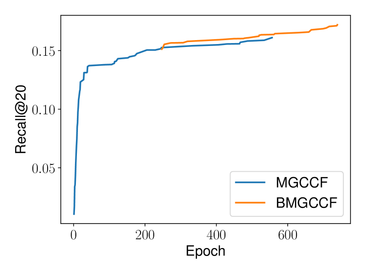
Figure 3: Training curve for MGCCF vs. BMGCCF (Amazon - CD).

The learning curve comparison for training the original model and the Bayesian version of the model is shown in Figure 3 for the Amazon CD dataset. We can observe that with our proposed solution, the training converges much faster. The Bayesian training framework also allows us to avoid overfitting in this case.

Conventional recommendation training procedure, especially in the implicit recommendation setting, treat all of the unobserved user-item interactions as negative feedback (demonstrating a lack of interest). Our proposed approach aims to learn which of these unobserved interactions are most likely to be false negatives. We analyze the overlap between the edges that we remove from the negative candidates set with the edges in the validation and test set. As shown in Table 4, our proposed Bayesian formulation is able to remove a significant percentage of test and validation edges from the negative sample pool.

Table 4: Edge overlap of the inferred graph with the test set.

	Am. CDs	Am. Books	Yelp2018	ML100Ks
BMGCF	20.6%	17.9%	13.6%	12.3%
BNGCF	23.4%	30.0%	13.3%	62.1%

5 CONCLUSION

In this paper, we propose the use of non-parametric modelling and inference of graphs for various learning tasks. In the proposed model, a higher edge weight between two nodes is more likely if the nodes are close in terms of a distance metric. An appropriate distance metric can be chosen depending on the learning task which results in flexible, task-specific design of learning algorithms. The proposed model is adapted to a Bayesian learning framework which aims to account for graph uncertainty. Experimental results demonstrate that the model can learn useful graphs that improve performance significantly over baseline algorithms for node classification, link prediction, and recommendation.

6 SUPPLEMENTARY MATERIAL

6.1 DESCRIPTION OF THE DATASETS

For the semi-supervised node classification and link prediction tasks, we conduct experiments on benchmark citation network datasets (Cora [Sen et al., 2008], Citeseer [Sen et al., 2008], and Pubmed [Namata et al., 2012]). In these datasets each node represents a research article and the undirected edges are formed according to citation links. Each node has a sparse bag-of-words feature vector derived from the keywords of the document. The node labels indicate the primary research topics addressed in the articles. The statistics of the citation datasets are summarized in Table 5.

Table 5: Statistics of evaluation datasets for node classification and generative graph models.

Dataset	# Classes	# Features	# Nodes	# Edges	Edge Density
Cora	7	1,433	2,485	5,069	0.04%
Citeseer	6	3,703	2110	3,668	0.04%
Pubmed	3	500	19,717	44,324	0.01%

For the experiments on the recommendation systems, we use four real-world and publicly available datasets: ML100K, Amazon-Books, Amazon-CDs and Yelp2018. For each dataset, we apply a pre-processing step to ensure that each user/item node in the dataset has sufficient interactions. We consider two threshold values $th_{1}$ and $th_{2}$, and filter out those users and those items with fewer than $th_{1}$ and $th_{2}$ interactions, respectively. The number of users and items after the preprocessing step are denoted by $|\mathcal{U}|$ and $|\mathcal{I}|$ respectively. The statistics of the preprocessed datasets are provided in Table 6.

Table 6: Statistics of evaluation datasets for recommender systems.

Dataset	$\bm{(th_{1},th_{2})}$	($|\mathcal{U}|$, $|\mathcal{I}|$)	# Edges	Edge Density
ML100K	(10, 10)	(897, 823)	36330	0.0716
CDs	(50, 20)	(2217, 2034)	68293	0.0151
Books	(250, 22)	(1608, 2270)	69782	0.0191
Yelp2018	(22, 35)	(2799, 1673)	119514	0.0255

6.2 GRAPH INFERENCE IN NON-PARAMETRIC MODEL

For completeness, we provide a brief summary of the graph inference task considered in the main paper. We solve for the maximizer $\widehat{\mathcal{G}}$ of the posterior distribution of the ‘true’ graph $\mathcal{G}$ as follows:

$$\widehat{\mathcal{G}} =\operatorname*{arg\,max}_{\mathcal{G}}p(\mathcal{G}|\mathcal{G}_{obs},\mathcal{D})\,,$$ (16)

Here, $\mathcal{G}_{obs}$ denotes the observed graph and $\mathcal{D}$ is additional information. In our non-parametric model, this is equivalent to solving the following optimization problem for the adjacency matrix $\mathbf{A}_{\widehat{\mathcal{G}}}$ of $\widehat{\mathcal{G}}$:

$$\mathbf{A}_{\widehat{\mathcal{G}}} =\operatorname*{arg\,min}_{\begin{subarray}{c}\mathbf{A}_{\mathcal{G}}\in\mathbf{R_{+}}^{N\times N},\\ \mathbf{A}_{\mathcal{G}}=\mathbf{A}_{\mathcal{G}}^{\top}\end{subarray}}\begin{aligned} &\|\mathbf{A}_{\mathcal{G}}\circ\mathbf{D}\|_{1,1}-\alpha\mathbf{1}^{\top}\log(\mathbf{A}_{\mathcal{G}}\mathbf{1})\\ &\quad\quad\quad\quad\quad\quad\quad+\beta\|\mathbf{A}_{\mathcal{G}}\|_{F}^{2}\,.\end{aligned}$$ (17)

We recall that $\mathbf{D}(\mathcal{G}_{obs},\mathcal{D})\geq\mathbf{0}$ is a symmetric pairwise distance matrix which measures the dissimilarity between the nodes. $\alpha$ and $\beta$ are the hyperparameters of the prior distribution of the random graph $\mathcal{G}$.

6.3 BAYESIAN GRAPH NEURAL NETWORK

This section summarizes the novel Bayesian Graph Neural Network algorithm and provides some additional results for the node classification task.

6.3.1 BGCN Algorithm

Algorithm 1 Bayesian GCN using non-parametric graph learning

1:  Input: $\mathcal{G}_{obs}$, $\mathbf{X}$, $\mathbf{Y_{\mathcal{L}}}$

2:  Output: $p(\mathbf{Z}|\mathbf{Y_{\mathcal{L}}},\mathbf{X},\mathcal{G}_{obs})$

3:  Train a node embedding algorithm using $\mathcal{G}_{obs}$ and $\mathbf{X}$ to obtain $\bm{z}_{i}$ for $1\leq i\leq N$. Compute $\mathbf{D}_{1}$ using (19).

4:  Train a base classifier using $\mathcal{G}_{obs}$, $\mathbf{X}$ and $\mathbf{Y_{\mathcal{L}}}$ to obtain $\hat{c}_{i}$ for $1\leq i\leq N$. Compute $\mathbf{D}_{2}$ using (20).

5:  Compute $\mathbf{D}$ using (18).

6:  Solve the optimization problem in (17) to obtain $A_{\widehat{\mathcal{G}}}$ (equivalently, $\widehat{\mathcal{G}}$).

7:  for $s=1$ to $S$ do

8:     Sample weights $\mathbf{W}_{s}$ using MC dropout by training a GCN over the graph $\widehat{\mathcal{G}}$.

9:  end for

10:  Approximate $p(\mathbf{Z}|\mathbf{Y_{\mathcal{L}}},\mathbf{X},\mathcal{G}_{obs})$ using (21).

We recall the notations from the main paper: $\mathbf{X}$ is the feature matrix of the nodes in the observed graph $\mathcal{G}_{obs}$ and $\mathbf{Y_{\mathcal{L}}}$ is the set of known training labels. $\mathbf{W}_{s}$ denotes the $s$-th sample of GCN weights trained on the inferred graph $\widehat{\mathcal{G}}$ from the non-parametric model. $\bm{z}_{i}$ represents any suitable embedding of node $i$ and $\hat{c}_{i}\in\{1,2,...K\}$ is the obtained label of $i$-th node from a baseline node classification algorithm. $\mathcal{N}_{i}=\{j|(i,j)\in\mathcal{E}_{\mathcal{G}_{obs}}\}\cup\{i\}$ is the neighbourhood of $i$-th node in $\mathcal{G}_{obs}$. The distance matrix $\mathbf{D}$ is defined as follows:

$$\mathbf{D}(\mathbf{X},\mathbf{Y_{\mathcal{L}}},\mathcal{G}_{obs}) =\mathbf{D}_{1}(\mathbf{X},\mathcal{G}_{obs})+\delta\mathbf{D}_{2}(\mathbf{X},\mathbf{Y_{\mathcal{L}}},\mathcal{G}_{obs})\,.$$ (18)

$$D_{1,ij}(\mathbf{X},\mathcal{G}_{obs}) =\|\bm{z}_{i}-\bm{z}_{j}\|^{2}\,,$$ (19)

$$D_{2,ij}(\mathbf{X},\mathbf{Y_{\mathcal{L}}},\mathcal{G}_{obs}) =\frac{1}{|\mathcal{N}_{i}||\mathcal{N}_{j}|}\displaystyle{\sum_{k\in\mathcal{N}_{i}}\sum_{l\in\mathcal{N}_{j}}}\mathbb{1}_{(\hat{c}_{k}\neq\hat{c}_{l})}\,.$$ (20)

Here, $\delta$ is a hyperparameter which controls the importance of $\mathbf{D}_{2}$ relative to $\mathbf{D}_{1}$. We need to compute the Monte Carlo approximation of the posterior distribution of labels, which is given as:

$$p(\mathbf{Z}|\mathbf{Y_{\mathcal{L}}},\mathbf{X},\mathcal{G}_{obs})\approx\dfrac{1}{S}\sum_{s=1}^{S}p(\mathbf{Z}|\mathbf{W}_{s},\mathcal{G}_{obs},\mathbf{X})\,.$$ (21)

Pseudocode for the proposed BGCN algorithm is provided in Algorithm 1.

6.3.2 Results on fixed training-test split from [Zhang et al., 2019]

Table 7: Classification accuracy (in $\%$) for Cora dataset.

Fixed split	5 labels	10 labels	20 labels
ChebyNet	67.9$\pm$3.1	72.7$\pm$2.4	80.4$\pm$0.7
GCN	74.4$\pm$0.8	74.9$\pm$0.7	81.6$\pm$0.5
GAT	73.5$\pm$2.2	74.5$\pm$1.3	81.6$\pm$0.9
BGCN	75.3$\pm$0.8	76.6$\pm$0.8	81.2$\pm$0.8
SBM-GCN	59.3$\pm$1.3	77.3$\pm$1.2	82.2$\pm$0.8
BGCN (ours)	76.0$\pm$1.1	76.8$\pm$0.9	80.3$\pm$0.6

Table 8: Classification accuracy (in $\%$) for Citeseer dataset.

Fixed split	5 labels	10 labels	20 labels
ChebyNet	53.0$\pm$1.9	67.7$\pm$1.2	70.2$\pm$0.9
GCN	55.4$\pm$1.1	65.8$\pm$1.1	70.8$\pm$0.7
GAT	55.4$\pm$2.6	66.1$\pm$1.7	70.8$\pm$1.0
BGCN	57.3$\pm$0.8	70.8$\pm$0.6	72.2$\pm$0.6
SBM-GCN	20.8$\pm$2.0	66.3$\pm$0.6	71.7$\pm$0.1
BGCN (ours)	59.0$\pm$1.5	71.7$\pm$0.8	72.6$\pm$0.6

Table 9: Classification accuracy (in $\%$) for Pubmed dataset.

Fixed split	5 labels	10 labels	20 labels
ChebyNet	68.1$\pm$2.5	69.4$\pm$1.6	76.0$\pm$1.2
GCN	69.7$\pm$0.5	72.8$\pm$0.5	78.9$\pm$0.3
GAT	70.0$\pm$0.6	71.6$\pm$0.9	76.9$\pm$0.5
BGCN	70.9$\pm$0.8	72.3$\pm$0.8	76.6$\pm$0.7
SBM-GCN	64.8$\pm$0.8	71.7$\pm$0.7	80.6$\pm$0.4
BGCN (ours)	73.3$\pm$0.7	73.9$\pm$0.9	79.2$\pm$0.5

In the main paper, we consider random partitioning of the nodes in training and test sets and report the average accuracies across different splits. We conduct another experiment where the same fixed training-test split of [Zhang et al., 2019] is used for 50 random intializations of the GCN weights. The classification results for this setting are provided in Tables 7, 8 and 9.

6.4 BAYESIAN VGAE ALGORITHM FOR LINK PREDICTION

We recall that the function $\mathcal{J}(\mathcal{G},\mathcal{G}_{obs})$ returns a graph such that the unobserved entries of the adjacency matrix of $\mathcal{G}_{obs}$ are replaced by the corresponding entries of $\mathcal{G}$. The distance matrix for the non-parametric graph inference is defined as:

$$D_{ij}(\mathbf{X},\mathcal{G}_{obs}) =\|\mathbb{E}_{q}[\bm{z}_{i}]-\mathbb{E}_{q}[\bm{z}_{j}]\|^{2}\,,$$ (22)

where, $q(\bm{Z}|\mathcal{G}_{obs},\mathbf{X})$ is the approximate posterior distribution of unsupervised node representations $\bm{Z}$ from a Variational Graph Auto-Encoder (VGAE) model. In the proposed Bayesian VGAE, the inference distribution is modelled as follows:

$$q(\bm{Z}|\mathcal{G}_{obs},\mathbf{X}) =\int q(\bm{Z}|\mathcal{J}(\mathcal{G},\mathcal{G}_{obs}),\mathbf{X})p(\mathcal{G}|\mathcal{G}_{obs},\mathbf{X})d\mathcal{G}\,,$$

$$\approx q(\bm{Z}|\mathcal{J}(\widehat{\mathcal{G}},\mathcal{G}_{obs}),\mathbf{X})\,.$$ (23)

Here $\widehat{\mathcal{G}}$ is the inferred graph from the non-parametric model. The resulting algorithm is summarized in Algorithm 2

Algorithm 2 Bayesian VGAE

1:  Input: $\mathcal{G}_{obs}$, $\mathbf{X}$

2:  Output: $q(\bm{Z}|\mathcal{G}_{obs},\mathbf{X})$

3:  Train a node embedding algorithm using $\mathcal{G}_{obs}$ and $\mathbf{X}$ to obtain $\bm{z}_{i}$ for $1\leq i\leq N$.

4:  Compute $\mathbf{D}$ using eq. (22).

5:  Solve the optimization problem in (17) to obtain $A_{\widehat{\mathcal{G}}}$ (equivalently, $\widehat{\mathcal{G}}$).

6:  Build a new graph $\mathcal{J}(\widehat{\mathcal{G}},\mathcal{G}_{obs})$ and train the auto-encoder on it to obtain $q(\bm{Z}|\mathcal{G}_{obs},\mathbf{X})$ (eq. (23)).

6.5 RECOMMENDATION SYSTEMS

6.5.1 Algorithm

We recall that $\{>_{u}\}_{train}$ is the set of training ranknings in observed graph $\mathcal{G}_{obs}$. The distance between the $u$-th user and the $i$-th item is defined as:

$$D_{u,i}(\{>_{\mathcal{U}}\}_{train},\mathcal{G}_{obs})=1-\frac{e_{u}\cdot e_{i}}{\lvert\lvert e_{u}\rvert\rvert_{2}\lvert\lvert e_{i}\rvert\rvert_{2}}\,.$$ (24)

Here, $e_{u}$ and $e_{i}$ are the representations from the base node embedding algorithm for the $u$-th user and the $i$-th item, respectively. We define $\widetilde{G}=\mathcal{J}_{r}(\mathcal{G},\mathcal{G}_{obs})$ by removing a fraction of links with the highest edge weights in $\mathcal{G}$ from the negative pool of interactions according to $\mathcal{G}_{obs}$. In the Bayesian version of the recommendation system, we need to compute:

$$p(\{>_{\mathcal{U}}\}_{test}|\{>_{\mathcal{U}}\}_{train},\mathcal{G}_{obs})=\int p(\{>_{\mathcal{U}}\}_{test}|\mathcal{G}_{obs},\mathbf{W})\,$$

$$\quad p(\mathbf{W}|\{>_{\mathcal{U}}\}_{train},\widetilde{\mathcal{G}})p(\mathcal{G}|\mathcal{G}_{obs},\{>_{\mathcal{U}}\}_{train})\,d\mathcal{G}\,d\mathbf{W}\,,$$

$$\approx p(\{>_{\mathcal{U}}\}_{test}|\mathcal{G}_{obs},\widehat{\mathbf{W}})\,.$$ (25)

We perform non-parametric graph inference to obtain $\widehat{\mathcal{G}}$, then compute $\widetilde{G}=\mathcal{J}_{r}(\widehat{\mathcal{G}},\mathcal{G}_{obs})$ and minimize the BPR loss to form the estimate of the weights:

$$\widehat{\mathbf{W}}=\operatorname*{arg\,max}_{\mathbf{W}}\hskip 5.0ptp(\mathbf{W}|\{>_{u}\}_{train},\widetilde{G})\,.$$ (26)

The resulting algorithm is summarized in Algorithm 3.

Algorithm 3 BPR loss minimization with non-parametric graph learning

1:  Input: $\{>_{u}\}_{train}$, $\mathcal{G}_{obs}$

2:  Output: $\{>_{u}\}_{test}$

3:  Train a base node embedding algorithm using $\mathcal{G}_{obs}$ and $\{>_{\mathcal{U}}\}_{train}$ to obtain embeddings for all users and items.

4:  Compute $\mathbf{D}$ as the pairwise cosine distance between the embeddings (eq. (24)).

5:  Solve the optimization problem in (17) using $\mathbf{D}$ to obtain $\widehat{\mathcal{G}}$.

6:  Form the modified graph $\widetilde{\mathcal{G}}=\mathcal{J}_{r}(\widehat{\mathcal{G}},\mathcal{G}_{obs})$.

7:  Minimize BPR loss with negative pool according to $\widetilde{\mathcal{G}}$ to obtain $\mathbf{\widehat{W}}$ (eq. (26)).

8:  Obtain the test set rankings using the embeddings to form $\{>_{\mathcal{U}}\}_{test}$ (eq. (25))

6.5.2 Definitions of the performance evaluation metrics

• Recall@k denotes the proportion of the true (preferred) items from the top-$k$ recommendation. For a user $u\in\mathcal{U}$, the algorithm recommends an ordered set of top-$k$ items $I_{k}(u)\in\mathcal{I}$. There is a set of true preferred items for a user $\mathcal{I}_{u}^{+}$ and a number of true positive $|\mathcal{I}_{u}^{+}\cap I_{k}(u)|$. The recall of a user is defined as follows :

  $$\mathrm{Recall@k}=\frac{|\mathcal{I}_{u}^{+}\cap I_{k}(u)|}{|\mathcal{I}_{u}^{+}|}$$

• NDCG@k: Normalized Discounted Cumulative Gain (NDCG) [Järvelin and Kekäläinen, 2000] computes a score for $I(u)$ which emphasizes higher-ranked true positives. $D_{k}(n)=(2^{rel_{n}}-1)/\log_{2}(n+1)$ accounts for a relevancy score $rel_{n}$. We consider binary responses, so we use a binary relevance score: $\mathrm{rel}_{n}=1$ if $i_{n}\in\mathcal{I}_{u}^{+}$ and 0 otherwise.

  $$\mathrm{NDCG}@k=\frac{\mathrm{DCG_{k}}}{\mathrm{IDCG_{k}}}=\frac{\sum_{n=1}^{|\mathcal{I}|}\mathrm{D}_{k}(n)[i_{n}\in\mathcal{I}_{u}^{+}]}{\sum_{n=1}^{|I_{k}(u)|}D_{k}(n)}$$

References

- [Bojchevski et al., 2018] Bojchevski, A., Shchur, O., Zügner, D., and Günnemann, S. (2018). NetGAN: Generating graphs via random walks. In Proc. Int. Conf. Machine Learning, pages 609–618.
- [Defferrard et al., 2016] Defferrard, M., Bresson, X., and Vandergheynst, P. (2016). Convolutional neural networks on graphs with fast localized spectral filtering. In Proc. Adv. Neural Inf. Proc. Systems, pages 3844–3852.
- [Dong et al., 2016] Dong, X., Thanou, D., Frossard, P., and Vandergheynst, P. (2016). Learning laplacian matrix in smooth graph signal representations. IEEE Trans. Sig. Proc., 64(23):6160–6173.
- [Duvenaud et al., 2015] Duvenaud, D., Maclaurin, D., et al. (2015). Convolutional networks on graphs for learning molecular fingerprints. In Proc. Adv. Neural Info. Proc. Systems, pages 2224–2232.
- [Gal and Ghahramani, 2016] Gal, Y. and Ghahramani, Z. (2016). Dropout as a Bayesian approximation: Representing model uncertainty in deep learning. In Proc. Int. Conf. Machine Learning, pages 1050–1059.
- [Grover and Leskovec, 2016] Grover, A. and Leskovec, J. (2016). node2vec: Scalable feature learning for networks. In Proc. ACM Int. Conf. Knowl. Disc. Data Mining, page 855–864.
- [Grover et al., 2019] Grover, A., Zweig, A., and Ermon, S. (2019). Graphite: iterative generative modeling of graphs. In Proc. Int. Conf. Machine Learning, pages 2434–2444.
- [Hamilton et al., 2017] Hamilton, W., Ying, R., and Leskovec, J. (2017). Inductive representation learning on large graphs. In Proc. Adv. Neural Inf. Proc. Systems, pages 1024–1034.
- [Hernández-Lobato and Adams, 2015] Hernández-Lobato, J. M. and Adams, R. (2015). Probabilistic backpropagation for scalable learning of Bayesian neural networks. In Proc. Int. Conf. Machine Learning, pages 1861–1869.
- [Järvelin and Kekäläinen, 2000] Järvelin, K. and Kekäläinen, J. (2000). IR evaluation methods for retrieving highly relevant documents. In Proc. Int. ACM SIGIR Conf. Research and Development in Information Retrieval, page 41–48.
- [Jiang et al., 2019] Jiang, B., Zhang, Z., Tang, J., and Luo, B. (2019). Graph optimized convolutional networks. arXiv e-prints : arXiv 1904.11883.
- [Kalofolias, 2016] Kalofolias, V. (2016). How to learn a graph from smooth signals. In Proc. Artificial Intell. and Statist., pages 920–929.
- [Kalofolias and Perraudin, 2019] Kalofolias, V. and Perraudin, N. (2019). Large scale graph learning from smooth signals. In Proc. Int. Conf. Learning Representations.
- [Kipf and Welling, 2016] Kipf, T. and Welling, M. (2016). Variational graph auto-encoders. In Proc. Bayesian Deep Learning Workshop, Adv. Neural Info. Process. Systems.
- [Kipf and Welling, 2017] Kipf, T. and Welling, M. (2017). Semi-supervised classification with graph convolutional networks. In Proc. Int. Conf. Learning Representations.
- [Li et al., 2016] Li, C., Chen, C., Carlson, D., and Carin, L. (2016). Pre-conditioned stochastic gradient Langevin dynamics for deep neural networks. In Proc. AAAI Conf. Artificial Intell., page 1788–1794.
- [Li et al., 2018] Li, Y., Vinyals, O., Dyer, C., Pascanu, R., and Battaglia, P. (2018). Learning deep generative models of graphs. In Proc. Int. Conf. Machine Learning.
- [Liao et al., 2019] Liao, R., Li, Y., Song, Y., Wang, S., Nash, C., Hamilton, W. L., Duvenaud, D., Urtasun, R., and Zemel, R. S. (2019). Efficient graph generation with graph recurrent attention networks. In Proc. Adv. Neural Info. Proc. Systems, pages 4255–4265.
- [Liu et al., 2019] Liu, J., Kumar, A., Ba, J., Kiros, J., and Swersky, K. J. (2019). Graph normalizing flows. In Proc. Adv. Neural Info. Proc. Systems, pages 13578–13588.
- [Ma et al., 2019] Ma, J., Tang, W., Zhu, J., and Mei, Q. (2019). A flexible generative framework for graph-based semi-supervised learning. In Proc. Adv. Neural Info. Proc. Systems, pages 3276–3285.
- [MacKay, 1996] MacKay, D. J. C. (1996). Maximum entropy and Bayesian methods, chapter Hyperparameters: Optimize, or Integrate Out?, pages 43–59. Springer Netherlands.
- [Malkov and Yashunin, 2020] Malkov, Y. A. and Yashunin, D. A. (2020). Efficient and robust approximate nearest neighbor search using hierarchical navigable small world graphs. IEEE Trans. Pattern Analysis and Machine Intell., 42(4):824–836.
- [Mehta et al., 2019] Mehta, N., Duke, L. C., and Rai, P. (2019). Stochastic blockmodels meet graph neural networks. In Proc. Int. Conf. Machine Learning, pages 4466–4474.
- [Monti et al., 2017] Monti, F., Bronstein, M., and Bresson, X. (2017). Geometric matrix completion with recurrent multi-graph neural networks. In Proc. Adv. Neural Info. Proc. Systems.
- [Namata et al., 2012] Namata, G., London, B., Getoor, L., and Huang, B. (2012). Query-driven active surveying for collective classification. In Proc. Workshop on Mining and Learning with Graphs, Int. Conf. Machine Learning.
- [Neal, 1992] Neal, R. M. (1992). Bayesian learning via stochastic dynamics. In Proc. Adv. Neural Inf. Proc. Systems, pages 475–482.
- [Pan et al., 2018] Pan, S., Hu, R., Long, G., Jiang, J., Yao, L., and Zhang, C. (2018). Adversarially regularized graph autoencoder for graph embedding. In Proc. Int. Joint Conf. Artificial Intell., pages 2609–2615.
- [Perozzi et al., 2014] Perozzi, B., Al-Rfou, R., and Skiena, S. (2014). Deepwalk: Online learning of social representations. In Proc. ACM SIGKDD Int. Conf. Knowl. Dis. Data Mining, pages 701–710.
- [Rendle et al., 2009] Rendle, S., Freudenthaler, C., Gantner, Z., and Schmidt-Thieme, L. (2009). BPR: Bayesian personalized ranking from implicit feedback. Proc. Conf. Uncertainty in Artificial Intell., pages 452–461.
- [Sen et al., 2008] Sen, P., Namata, G., et al. (2008). Collective classification in network data. AI Magazine, 29(3):93.
- [Simonovsky and Komodakis, 2018] Simonovsky, M. and Komodakis, N. (2018). GraphVAE: Towards generation of small graphs using variational autoencoders. In Proc. Int. Conf. Artificial Neural Networks, pages 412–422.
- [Sun et al., 2019] Sun, J., Zhang, Y., Ma, C., Coates, M., Guo, H., Tang, R., and He, X. (2019). Multi-graph convolution collaborative filtering. In Proc. IEEE Int. Conf. Data Mining, pages 1306–1311.
- [Sun et al., 2017] Sun, S., Chen, C., and Carin, L. (2017). Learning structured weight uncertainty in Bayesian neural networks. In Proc. Artificial Intell. and Statist., pages 1283–1292.
- [Tang and Liu, 2011] Tang, L. and Liu, H. (2011). Leveraging social media networks for classification. Data Mining and Knowledge Discovery, pages 447–478.
- [Tian et al., 2019] Tian, Y., Zhao, L., Peng, X., and Metaxas, D. (2019). Rethinking kernel methods for node representation learning on graphs. In Proc. Adv. Neural Info. Proc. Systems, pages 2088–2099.
- [Tiao et al., 2019] Tiao, L. C., Elinas, P., Nguyen, H., and Bonilla, E. V. (2019). Variational spectral graph convolutional networks. In Proc. Graph Representation Learning Workshop, Adv. Neural Info. Proc. Systems.
- [van den Berg et al., 2018] van den Berg, R., Kipf, T. N., and Welling, M. (2018). Graph convolutional matrix completion. In Proc. ACM Int. Conf. Knowl. Disc. Data Mining.
- [Veličković et al., 2018] Veličković, P., Cucurull, G., Casanova, A., Romero, A., Liò, P., and Bengio, Y. (2018). Graph attention networks. In Proc. Int. Conf. Learning Representations.
- [Wang et al., 2017] Wang, H., Wang, J., Wang, J., Zhao, M., Zhang, W., Zhang, F., Xie, X., and Guo, M. (2017). GraphGAN: Graph representation learning with generative adversarial nets. In Proc. AAAI Conf. Artificial Intell., pages 2508–2515.
- [Wang et al., 2019] Wang, X., He, X., Wang, M., Feng, F., and Chua, T.-S. (2019). Neural graph collaborative filtering. In Proc. Int. ACM SIGIR Conf. Research and Development Info. Retrieval, pages 165–174.
- [Wijesinghe and Wang, 2019] Wijesinghe, W. O. K. A. S. and Wang, Q. (2019). DFNets: Spectral CNNs for graphs with feedback-looped filters. In Proc. Adv. Neural Info. Proc. Systems, pages 6009–6020.
- [Ying et al., 2018] Ying, R., He, R., Chen, K., Eksombatchai, P., Hamilton, W. L., and Leskovec, J. (2018). Graph convolutional neural networks for web-scale recommender systems. In Proc. ACM Int. Conf. Knowl. Disc. Data Mining, pages 974–983.
- [You et al., 2018] You, J., Ying, R., Ren, X., Hamilton, W. L., and Leskovec, J. (2018). GraphRNN: Generating realistic graphs with deep auto-regressive models. In Proc. Int. Conf. Machine Learning, pages 5708–5717.
- [Zhang et al., 2019] Zhang, Y., Pal, S., Coates, M., and Üstebay, D. (2019). Bayesian graph convolutional neural networks for semi-supervised classification. In Proc. AAAI Conf. Artificial Intell., pages 5829–5836.
- [Zheng et al., 2018] Zheng, L., Lu, C.-T., Jiang, F., Zhang, J., and Yu, P. S. (2018). Spectral collaborative filtering. In Proc. ACM Conf. Recommender Systems.
- [Zhuang and Ma, 2018] Zhuang, C. and Ma, Q. (2018). Dual graph convolutional networks for graph-based semi-supervised classification. In Proc. World Wide Web Conf., page 499–508.