Detecting and tracking bacteria with quantum light

Abstract

The field of quantum sensing aims at improving the detection and estimation of classical parameters that are encoded in physical systems by resorting to quantum sources of light and quantum detection strategies. The same approach can be used to improve the current classical measurements that are performed on biological systems. Here we consider the scenario of two bacteria (E. coli and Salmonella) growing in a Luria Bertani broth and monitored by classical spectrophotometers. Their concentration can be related to the optical transmissivity via the Beer-Lambert-Bouguer’s law and their growth curves can be described by means of Gompertz functions. Starting from experimental data points, we extrapolate the growth curves of the two bacteria and we study the theoretical performance that would be achieved with a quantum setup. In particular, we discuss how the bacterial growth can in principle be tracked by irradiating the samples with orders of magnitude fewer photons, identifying the clear superiority of quantum light in the early stages of growth. We then show the superiority and the limits of quantum resources in two basic tasks: (i) the early detection of bacterial growth and (ii) the early discrimination between two bacteria species.

I Introduction

Growth curves are found in a wide range of disciplines, such as fishery research, crop science, and other areas of biology ref1 . They have for a long time been used to study the dynamics of the populations of bacteria. These curves typically show an initial lag time after which the concentration (or number of organisms) starts to increase exponentially towards a maximal saturation value; in this final stationary phase the growth rate gradually decreases to zero as the asymptote is reached. This overall process results into a typical sigmoidal curve that has been represented by various mathematical models ref3 . The parameters of this curve depend on the specific process under study, be it bacterial growth in samples or dose-mortality relations ref2 .

In today’s biology and chemistry laboratories, the spectrophotometer is the instrument that is used to measure bacterial concentrations and therefore track their growth. This is an optical instrument which measures the transmission $\eta\in[0,1]$ of visible, UV or infrared light, through a sample. More precisely, it measures the “optical absorbance” $A:=-\log_{10}\eta$ dB also known as “optical density” (we assume negligible scattering from the sample). Its basic principle is the well-known Beer-Lambert-Bouguer law Bouguer ; Lambert ; Beer , which relates the optical absorbance of a sample to its concentration Ingle88 . More precisely, the absorbance $A$ at some specific wavelength $\lambda$ is equal to the concentration of the sample $C$ (in units of $\mathrm{mol}/\mathrm{m}^{3}$) times the length $l$ of the optical path (in units of $\mathrm{m}$) times the molar extinction coefficient $\varepsilon$ specific of the substance (in units of $\mathrm{m}^{2}/\mathrm{mol}$). Thus, we have the formula $A=\varepsilon lC$ or equivalently $\eta=10^{-\varepsilon lC}$. In a standard setup, where $\varepsilon$ and $l$ are fixed, the absorbance is the relevant quantity to be considered for tracking bacterial growth.

The two main types of spectrophotometers are single- and double-beam. The first design measures only the light intensity at the output of the sample, while the second measures the ratio of the light intensities at the output of two separate paths, one sent through the sample and the other one sent through a reference or blank. It is important to estimate the typical number of photons that are irradiated by these devices for their readout. To give an idea of the order of magnitude, we perform a simple calculation based on one of the spectrophotometers that we used for our experimental data (Ultraspect 2100 pro Amersham Bioscience). This employs a Xenon light source at $600$nm with an average of power $10$W, flashing at a frequency of $25$Hz, corresponding to about $0.4$J per flash. A typical measurement involves about $6$ flashes for a total time of about $1/4$ of a second, corresponding to about $2.4$J of energy $E$ irradiated over the sample. From Planck’s law $E=nhc/\lambda$, we can derive the staggering value of $n\simeq 10^{19}$ thermally-distributed photons at $600$nm wavelength.

The irradiation of such a high energy is a potential disadvantage for this instrument. In fact, a very high number of photons can be destructive, especially if the sample contains photosensitive bacteria, fragile proteins or DNA/RNA. Furthermore, there are other limitations to account for in current spectrophotometers. One problem is the low sensitivity of the instrument, which is often inadequate for good readouts of low concentrations, a task which is very important in scenarios such as early disease detection or food poisoning. Because of this poor performance, researchers may need to re-prepare their samples many times to get a good statistical estimate.

In the present work, we discuss how the use of quantum resources can drastically reduce the number of photons that are required for readouts of bacterial concentration. Collecting experimental data with standard spectrophotometers, first we study the typical realistic errors affecting these classical instruments in tracking the growth of bacterial species (E. coli and Salmonella). From this data, we extrapolate the functional forms of the bacterial growth curves, which are then used in our theoretical simulation of an optimal quantum setup. We show that similar performances can be achieved by using quantum designs that employ sources of light with orders of magnitude fewer photons, when suitably combined with corresponding optimal quantum detections.

Depending on the working regime (lower or higher concentrations), there is a preferable semiclassical or truly quantum state to be used for the input light. At higher concentrations, one needs to consider coherent states irradiating a relatively high mean number of photons per readout (e.g., of the order of $10^{4}$). This source is studied in combination with an optimal quantum detection at the output. It represents our semiclassical benchmark which bounds the performance of any other classical source (even when the output detection is quantum). We also discuss how its performance can be achieved by using a double-beam setup where asymmetrically-correlated two-mode thermal states are prepared at the input and photon-resolving measurements are performed at the output.

Our results show that the use of truly quantum states is limited to low concentrations, i.e., during the early phase of bacterial growth. Considering this initial phase and assuming a small number of photons irradiated over the sample, the performance of optimal quantum states in estimating the concentration clearly outperforms the semiclassical benchmark based on coherent states. In general, the optimal quantum states can be engineered as suitable superpositions of number states AdessoIlluminati ; ReviewNEW and their quantum measurement is the optimal one which minimizes the quantum Cramer Rao bound (QCRB) SamMETRO . In practice, we also analyze the performance of quantum states (squeezed vacua) that can be easily engineered in the lab, showing that they offer a similar quantum advantage as the optimal quantum probes.

Because quantum advantage is relevant at low concentrations, it is therefore important in tasks of early bacterial detection. We therefore study the task of the early detection of the growth of E. coli in a sample, and the task of the early discrimination between the growth of two different bacterial species (E. coli and Salmonella). In both cases, we are able to show the advantage of the optimal and practical quantum sources with respect to the semiclassical benchmark (coherent states), both in terms of reducing the time for detecting bacterial growth and decreasing the error probability in the discrimination between two different species.

The manuscript is organized as follows. In Sec. II we describe our classical experiments for tracking the growth of E. coli and Salmonella via standard spectrophotometer in typical lab conditions. Then, in Sec. III, we study the performance of a theoretical quantum-enhanced model of spectrophotometer based on semiclassical or truly quantum sources and output quantum detection. In Sec. IV we study early detection and discrimination of bacteria. Finally, Sec. V is for conclusions.

II Experimental growth curves with classical instruments

We have performed two different experiments. In the first experiment, we considered a single bacterial species (E. coli, MRE600) Meier . The results were averaged over the strain so as to consider an average behavior. In the second experiment, we instead considered two different species of bacteria (E. coli BW25113) and Salmonella (enterica serovar Typhimurium ATCC1428 strain) whose growth behaviors were analyzed separately. In all cases, the bacteria were first grown in a Luria Bertani broth at $30^{\circ}$C and then suitably diluted for subsequent measurements. Their concentration (optical absorbance) were measured by using classical spectrophotometers. Finally, the outcomes were statistically post-processed into experimental growth curves. See Methods for more details.

From the experimental data, we extrapolated analytical forms for the growth curves, according to the Gompertz function Gompertz1825 ; ref3 . This function relates the concentration/absorbance $A$ of the sample to time $t$, as follows

$$A=a\exp[-\exp(b-ct)],$$ (1)

where $a$, $b$, and $c$ are parameters to be interpolated from the data. Note that the Gompertz function can also be re-written as (ref3, , Eq. (11))

$$A=a\exp\left\{-\exp\left[\frac{\mu e}{a}(\theta-t)+1\right]\right\}+A_{\text{bk}},$$ (2)

where $a$ is the asymptotic absorbance at infinite time $t\rightarrow\infty$, $\mu:=ac/e$ is the rate of growth in the linear region, and $\theta:=(b-1)/c$. Here we have also added an additional offset $A_{\text{bk}}$ accounting for non-zero mean absorbance of the blank sample (i.e., non-unit transmissivity $\eta_{\text{bk}}$ of the media holding the species under study).

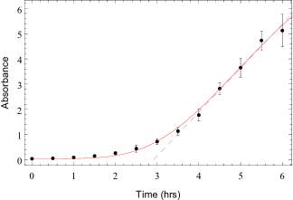
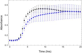
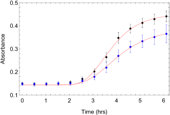
The data of the first experiment is shown in Fig. 1. At each time, 24 data points were measured and post-processed into a mean value plus an error bar. Data was then used to interpolate a Gompertz function with suitable parameters. The entire data of the second experiment is shown in Fig. 2. At each time, 18 data points per species were measured and post-processed as before. In particular, in Fig. 3 we zoom on the first six hours, where the two growth curves for E. coli and Salmonella are more distinguishable. These experimental curves have been interpolated by two Gompertz functions.

Figure 1: Growth curve of E. coli (wild type MRE 600) in terms of optical absorbance versus time (hours). We show the experimental data, suitably post-processed into a mean curve with error bars corresponding to one standard deviation. The data is then interpolated by the Gompertz function (red line) given by Eq. (2) with parameters $a\simeq 9.4$, $\mu\simeq 1.7$, $\theta\simeq 2.9$ and $A_{\text{bk}}\simeq 0.036$. For completeness, we also show the linear phase $(t-\theta)\mu$ of the growth (dashed blue line). This linear phase occurs after the latency phase and before the saturation phase of the sigmoid.

Figure 2: Growth curves of E. coli (black points) and Salmonella (blue points) in terms of optical absorbance versus time (hours). We show the experimental data, post-processed into mean curves with error bars corresponding to one standard deviation.

Figure 3: Growth curves of E. coli (black points) and Salmonella (blue points) in terms of optical absorbance versus time (hours). We zoom the experimental data of Fig. 2 for times up to six hours. The two sets of data points are interpolated by two Gompertz functions with parameters $\{a,\mu,\theta\}\simeq\{0.309,0.139,2.634\}$ for E. coli and $\{a,\mu,\theta\}\simeq\{0.242,0.0882,2.672\}$ for Salmonella. In both cases, the blank has mean absorbance $A_{\text{bk}}\simeq 0.144$ (corresponding to a blank transmissivity $\eta_{\text{bk}}\simeq 0.717$).

III Theoretical performance with a quantum setup

We now consider the theoretical performance that is achievable by using a semiclassical or a quantum source at the input, combined with optimal quantum detection at the output. Our first aim is to show that a semiclassical or fully quantum setup can achieve an accuracy that is comparable with the typical performance of a classical spectrophotometer while using orders of magnitude fewer photons. As semiclassical sources, we consider single-mode coherent states and also their approximation by means of two-mode correlated thermal states. As truly quantum sources we consider optimal single-mode states, such as number states and their superpositions AdessoIlluminati . To explore the limits achievable by these sources in the estimation of optical absorbance, we consider the QCRB SamMETRO . For a fixed source (input state) and number $N$ of probings of the sample, this bound provides the minimum error-variance that we could achieve by optimizing over all possible quantum measurements at the output.

First of all, for our purposes, we need to connect the error (standard deviation) $\sigma_{\eta}$ affecting the transmissivity $\eta$ of the sample to the error (standard deviation) $\sigma_{A}$ associated with the absorbance $A=-\log_{10}\eta$. A simple calculation provides $\sigma_{A}\simeq\sigma_{\eta}/(\bar{\eta}\ln 10)$, where $\bar{\eta}$ is the mean value of the transmissivity, corresponding to $\bar{\eta}=10^{-\bar{A}}$, where $\bar{A}$ is the mean value of the absorbance. This approximation is justified by the so-called delta-method DM1 ; DM1b ; DM2 (see Methods for more details). In our theoretical simulation for the quantum setup, we assume that the experimental mean value $\bar{A}$, which is well-approximated by the Gompertz function, represents the actual physical value $A$ of the absorbance. Correspondingly, we assume that the mean value $\bar{\eta}=10^{-\bar{A}}$ corresponds to the actual physical value of the transmissivity. As a result, we may modify the previous expansion into the following form

$$\sigma_{A}\simeq\frac{\sigma_{\eta}}{\eta\ln 10}.$$ (3)

The next step is to assume the QCRB for the computation of $\sigma_{\eta}$. Assume that the sample can be approximately modelled as a pure-loss bosonic channel $\mathcal{E}_{\eta}$ with transmissivity $\eta$. This channel/sample is probed by $N$ quantum states $\rho_{\bar{n}}^{\otimes N}$ which irradiate a total of $\bar{n}_{\text{tot}}:=N\bar{n}$ mean number of photons, where $\bar{n}$ is the mean number of photons per state. Assuming an optimal measurement of the output states $\rho_{\text{out}}^{\otimes N}$, we can construct an unbiased estimator $\hat{\eta}$ of $\eta$. This estimator is subject to an error-variance given by the QCRB

$$\sigma_{\eta}^{2}\geq\frac{1}{NH_{\eta,\bar{n}}},$$ (4)

where $H_{\eta,\bar{n}}$ is the quantum Fisher information (QFI) SamMETRO , to be computed on the single-copy output state $\rho_{\text{out}}:=\mathcal{E}_{\eta}(\rho_{\bar{n}})$. When $\rho_{\text{out}}$ is a Gaussian state RMP , we can easily compute the QFI from the fidelity, according to the general formulae in Ref. Banchi .

Combining Eqs. (3) and (4), we may write the following standard deviation error for the absorbance

$$\sigma_{A}\gtrsim\left[\frac{1}{\eta(\ln 10)\sqrt{NH_{\eta,\bar{n}}}}\right]_{\eta=10^{-A}}.$$ (5)

The explicit expression of the QFI $H_{\eta,\bar{n}}$ depends on the transmissivity $\eta$ and the single-copy input state $\rho_{\bar{n}}$. Assuming a single-beam configuration where the light emitted by the source can be described by a coherent state $\rho_{\bar{n}}=\left|\sqrt{\bar{n}}\right\rangle\left\langle\sqrt{\bar{n}}\right|$ irradiating $\bar{n}$ mean photons, we have $H_{\eta,\bar{n}}=\bar{n}/\eta$ MonrasParis , so that

$$\sigma_{A}\gtrsim\frac{1}{\ln 10}\sqrt{\frac{10^{A}}{\bar{n}_{\text{tot}}}}.$$ (6)

This performance can equivalently be achieved in a double-beam configuration where a two-mode correlated thermal state is prepared in a very asymmetric way, so that one mode is faint and the other is highly energetic (see Ref. Sped for more details on this equivalence). The faint mode is sent through the sample while the energetic one is directly sent to the output measurement, where both the output modes are subject to photon counting (see Methods for more details).

The optimal quantum performance corresponds to MonrasParis $H_{\eta,\bar{n}}=\bar{n}[\eta(1-\eta)]^{-1}$, which is reached by input number states or suitable superpositions AdessoIlluminati . By substitution into Eq. (5), we derive the following improved error and its expansion at low absorbance

$$\sigma_{A} \gtrsim\frac{1}{\ln 10}\sqrt{\frac{10^{A}-1}{\bar{n}_{\text{tot}}}}$$ (7)

$$\simeq\sqrt{\frac{A}{\bar{n}_{\text{tot}}\ln 10}}+\mathcal{O}(A^{3/2}).$$ (8)

An important observation about the standard deviations in Eqs. (6) and (7) is the fact that they depend on the energy of the input via the mean total number of photons $\bar{n}_{\text{tot}}=N\bar{n}$. This means that these quantities do not change if we consider a single energetic state ($N=1$, $\bar{n}=\bar{n}_{\text{tot}}$) or a large number of lower-energy states so that $N\gg 1$ and $\bar{n}\ll\bar{n}_{\text{tot}}$ with $N\bar{n}=\bar{n}_{\text{tot}}$ (assuming that the total measurement time of this second option is reasonable). This is particularly useful for the truly quantum resources which are typically limited to $1$ photon or less; for these, we implicitly assume the condition of low-energy single-copy states so that we increase the total energy by increasing the number of copies $N$. Furthermore, in the regime of large $N$, the QCRB is known to be achievable SamMETRO ; Paris ; ReviewNEW and the optimal detection strategy can be realized by using local quantum measurements (i.e., performed over the single copies) combined with adaptive estimators asy1 ; asy2 .

Figure 4: Theoretical growth curves achievable by using coherent states and an optimal output detection, reaching the QCRB in Eq. (6). We plot the mean bacterial growth (solid red curve) as given by the Gompertz function from Fig. 1. Then, we consider the error bars (at one standard deviation) given by coherent states with $\bar{n}_{\text{tot}}=100$ (solid black lines), $\bar{n}_{\text{tot}}=1000$ (dashed black lines) and $\bar{n}_{\text{tot}}=10000$ (dotted black lines).

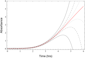
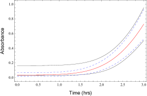
We show our numerical results in Figs. 4-5, considering the mean growth curve of E. coli approximated by the Gompertz function plotted in Fig. 1. In Fig. 4 we show the error bars (at one standard deviation) that we would obtain by using coherent states for different values of total energy irradiated. As we can see from the figure, the error bars are narrow at low absorbances for which we can use relatively few photons, while they quickly increase at higher values of the absorbance, for which we need to consider energetic coherent states. At high absorbance, the performance of coherent states approximates the quantum limit, as we can see by comparing Eqs. (6) and (7) for large $A$. This means that, for this regime, it makes little sense to consider truly quantum states such as number states and the best strategy is to use coherent states with high energy.

However, different is the case for low absorbances/concentrations. As we can see from Fig. 5, at the early stage of bacterial growth, i.e., during the latency phase of the sigmoid, the use of optimal quantum sources gives a non-trivial advantage with respect to coherent states, for the same mean number of photons irradiated over the sample. In other words, the initial latency phase, i.e., the low-concentration regime, is the most interesting from the quantum point of view. Note the asymmetric behavior of the error bars when the absorbance is close to zero. This is due to the fact that the Gaussian distribution needs to be truncated. Start with a Gaussian distribution with mean value $\bar{A}$ and standard deviation $\sigma_{A}$, and imposes a $1$-sided truncation at the origin. Then the mean value and standard deviation of the new distribution are given by

$$\bar{A}^{\prime}=\bar{A}+g(\omega)\sigma_{A},~{}~{}\sigma_{A}^{\prime}=\sigma_{A}\sqrt{1+\omega g(\omega)-g(\omega)^{2}},$$ (9)

where $\omega:=-\bar{A}/\sigma_{A}$ and

$$g(x):=\frac{2\mathcal{N}(x)}{1-\operatorname{erf}\left(x/\sqrt{2}\right)},$$ (10)

with $\mathcal{N}(x)$ being the standard normal distribution and $\operatorname{erf}(x):=2\pi^{-1/2}\int_{0}^{x}e^{-x^{2}}dx$ the error function.

Figure 5: Theoretical growth curves at low values of absorbance (latency phase). By fixing $\bar{n}_{\text{tot}}=20$ photons, we compare the optimal error bars achievable by coherent states (solid black lines) and those achievable by the optimal quantum states (dashed blue lines). The mean growth curve (solid red line) is the Gompertz function from Fig. 1.

Besides investigating the optimal quantum limit, in our following analysis we also explore the performance of a practical quantum source, as represented by an input squeezed vacuum state. This is a zero-mean Gaussian state with covariance matrix $\mathrm{diag}(r,r^{-1})$, where $r\leq 1$ represents the squeezing parameter (in the $q$-quadrature). It is easy to see that its mean number of photons depends on $r$ and is given by $\bar{n}=(1-r)^{2}/(4r)$. From the literature ReviewNEW ; MonrasParis , we know that the performance of this input state for bosonic loss estimation is close to optimal when $\bar{n}$ is low. In particular, adapting the result from Ref. MonrasParis , the QFI takes the form

$$H_{\eta,\bar{n}}=\frac{1}{\eta}\left[\frac{\bar{n}-2\bar{n}\eta(1-\eta)}{(1-\eta)[1+2\bar{n}\eta(1-\eta)]}\right],$$ (11)

which can be used in Eq. (5) to derive the performance of the squeezed vacuum probe.

Note that, in this case, parameters $\bar{n}$ and $N$ are not simply combined as before, but we need to fix $N$ and use $\bar{n}=\bar{n}_{\text{tot}}/N$ in Eq. (11). In this case, we get a lower bound from Eq. (5) which depends on $A$ and $\bar{n}_{\text{tot}}$. More precisely, one may start by fixing the amount of decibels that can be realized for the squeezed probes. Even though values up to $9.3$ dB are currently realizable SqueezingTobias , in our study we will consider the case of a relatively cheap source with just $1$ dB of squeezing, so that $r=10^{-1/10}\simeq 0.794$ and we have $\bar{n}\simeq 0.013$ mean photons per probe. For instance, this means that using a total of $\bar{n}_{\text{tot}}=20$ mean photons corresponds to irradiating $N=1500$ probes. Number of probes in the order of $10^{3}-10^{5}$ requires a negligible time with respect to the time-scale associated with the bacterial growth. For instance, using a clock rate and a detector at $1$ MHz, these probes are generated and detected in about $1-100$ ms.

IV Quantum-enhanced early detection

IV.1 Detecting growth of E. coli

Once it is understood that the initial phase of the bacterial growth is the most interesting one from the quantum point of view, we therefore consider the task of early detection. This consists in distinguishing whether bacteria are growing or not in the sample. More precisely, we study the time required for successfully discriminating whether the sample is blank or contains E. coli growing in accordance with the experimental data of our first experiment (see Fig. 1). As a first step, we translate the absorbance data $A$ into transmissivity data $\eta=10^{-A}$ which is the quantity physically measured by the instrument (and following a Gaussian distribution under the assumption of many measurements). During the first phase of the growth (up to $3$ hours), we interpolate the experimental data with a theoretical curve of the form $\eta(t)=\eta_{\text{bk}}-ct^{2}+dt^{3}$, where $\eta_{\text{bk}}$ is the transmissivity of the blank sample, while $c$ and $d$ are suitable constants. From the experimental data of the absorbance (see Fig. 1), we therefore retrieve the corresponding decay in optical transmissivity $\eta$ versus time $t$ (hours) for E. coli. We find $\eta_{\text{bk}}\simeq 0.92$, $c\simeq 0.1$ and $d\simeq 0.0088$ for the cubic theoretical curve $\eta(t)$.

Figure 6: Decay of transmissivity due to the growth of E. coli versus time $t$ (black points) compared with the constant transmissivity of a blank sample (blue points). The sample is monitored by irradiating a total of $\bar{n}_{\text{tot}}=150$ photons for each reading. Error bars refer to one standard deviation as given by the QCRB. In (a) we consider coherent states as the input source, while in (b) we consider optimal quantum states. The mean decay (red line) is given by the curve $\eta(t)$ extrapolated by the experimental data and described in the main text.

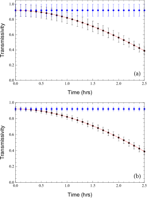
Using the curve $\eta(t)$ we then consider the error bars achievable by an optimal quantum setup (in terms of source and detection) and those that are instead achievable by a semi-classical setup where the source is prepared in coherent states and the output is optimally detected by a quantum measurement. As previously discussed, the latter is a benchmark which bounds the ultimate theoretical performance of any classical setup, i.e., based on classical sources (coherent/thermal states) combined with classical receivers (e.g., non-photon-resolving intensity measurements).

Using the QCRB for coherent states $\sigma_{\eta}\geq\sqrt{\eta/\bar{n}_{\text{tot}}}$ and the QCRB for the optimal quantum states $\sigma_{\eta}\geq\sqrt{\eta(1-\eta)/\bar{n}_{\text{tot}}}$, we plot the curves in Fig. 6. This figure already qualitatively shows that truly quantum sources can perform much better at short times. Below we make this observation quantitative by computing the corresponding error probabilities in detecting the bacterial growth as a function of time.

Let us assume that at time $t$, we can perform a sufficiently large number of measurements, so that the QCRB is well-approximated (we use many probes $N$, each with small mean number of photons $\bar{n}$ such that the total $N\bar{n}$ matches the fixed energetic constraint $\bar{n}_{\text{tot}}$). At each reading time $t$, the data points $\{\eta_{k}\}_{k=1}^{N}$ provided by the quantum measurement are used to build an estimator $\hat{\eta}$ of the transmissivity $\eta(t)$ whose error $\sigma_{\eta}$ is given by the QCRB for $\bar{n}_{\text{tot}}$ mean total number of photons irradiated by the source. Assume that the estimator approximately follows a Gaussian distribution in $\eta$ as a result of the central limit theorem (e.g., the estimator may be based on the arithmetic mean of the outcomes which, in turn, are identically and independently distributed). Furthermore, for increasing $\bar{n}_{\text{tot}}$, the standard deviation $\sigma_{\eta}$ of this distribution is sufficiently small, so that the truncation of the tails at the border of the finite segment $0\leq\eta\leq 1$ becomes a relatively small effect.

For the null hypothesis $H_{0}$ (no growth), the estimator $\hat{\eta}$ is centered around $\eta_{\text{bk}}$ according to a Gaussian distribution $p_{0}(\eta)$ with standard deviation $\sigma_{\eta_{\text{bk}}}$. For the alternative hypothesis $H_{1}$ (yes growth), the estimator $\hat{\eta}$ will be instead centered around $\eta(t)\leq\eta_{\text{bk}}$ according to a Gaussian distribution $p_{1}(\eta)$ with standard deviation $\sigma_{\eta(t)}$. We can therefore consider a decision test with threshold $0\leq\tau\leq 1$: if $\hat{\eta}\geq\tau$ we accept the null hypothesis $H_{0}$, while if $\hat{\eta}<\tau$ we accept the alternative hypothesis $H_{1}$. Consequently, there are associated false-positive $p_{\text{FP}}$ and false-negative $p_{\text{FN}}$ error probabilities

$$p_{\text{FP}} :=\text{prob}(H_{1}|H_{0})=\mathcal{N}_{0}^{-1}\int_{0}^{\tau}p_{0}(\eta)d\eta,$$ (12)

$$p_{\text{FN}} :=\text{prob}(H_{0}|H_{1})=\mathcal{N}_{1}^{-1}\int_{\tau}^{1}p_{1}(\eta)d\eta,$$ (13)

where the normalization factors $\mathcal{N}_{i}:=\int_{0}^{1}p_{i}(\eta)d\eta$ for $i=0,1$ are due to the truncation at the border. Under this hypothesis, we may compute

$$p_{\text{FP}}(\tau) =\frac{1}{2\mathcal{N}_{0}}\left\{\operatorname{erf}\left[\frac{\eta_{\text{bk}}}{\sqrt{2}\sigma_{\eta_{\text{bk}}}}\right]-\operatorname{erf}\left[\frac{\eta_{\text{bk}}-\tau}{\sqrt{2}\sigma_{\eta_{\text{bk}}}}\right]\right\},$$ (14)

$$p_{\text{FN}}(\tau,t) =\frac{1}{2\mathcal{N}_{1}}\left\{\operatorname{erf}\left[\frac{\eta(t)-\tau}{\sqrt{2}\sigma_{\eta(t)}}\right]-\operatorname{erf}\left[\frac{\eta(t)-1}{\sqrt{2}\sigma_{\eta(t)}}\right]\right\}.$$ (15)

Figure 7: Early detection of growth of E. coli. We plot the error probability versus time $t$ (hours) for the semiclassical case of a coherent-state source (dashed line), an optimal quantum source (solid black line) and a practical squeezed quantum source (solid purple line), all of them irradiating $\bar{n}_{\text{tot}}=150$ mean total photons over the sample at each reading time. In particular, we choose $1$dB of squeezing for the squeezed vacuum probe, so that we have $\bar{n}\simeq 1.33\times 10^{-2}$ mean photons per mode, which requires the use of $N=11267$ probes (so as to irradiate $150$ mean photons overall). In panel (a) we consider the false-negative error probability $p_{\text{FN}}$ over time $t$, fixing the value of false-positive error probability to $p_{\text{FN}}=1\%$. In panel (b) we plot the mean error probability $p_{\text{mean}}$ over time $t$. For both symmetric and asymmetric testing, we can see how the optimal and practical quantum sources allow one to detect bacterial growth much earlier than the semiclassical benchmark (at about $1$ hour instead of $2$ hours).

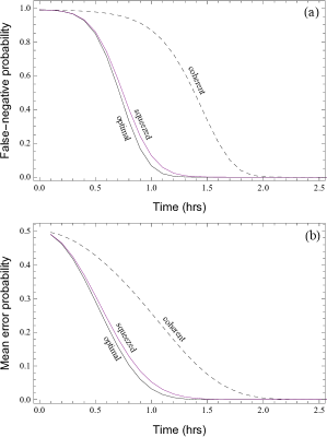
We have now two possible types of testing. In asymmetric testing, we fix a tolerable value for the false positives. This means we fix a value for $p_{\text{FP}}$ and, therefore, for the threshold parameter $\tau$, which can be expressed as an inverse function $\tau=\tau(p_{\text{FP}})$. We then replace $\tau$ in $p_{\text{FN}}(\tau,t)$, and study the false-negative error probability $p_{\text{FN}}$ over time. In symmetric testing, we instead assume that the two error probabilities have equal Bayesian costs. In the case of the same priors, the quantity of interest is therefore the mean error probability

$$p_{\text{mean}}(t):=\min_{\tau}\frac{p_{\text{FP}}(\tau)+p_{\text{FN}}(\tau,t)}{2}.$$ (16)

The numerical results are shown in Fig. 7 for both asymmetric and symmetric testing. In the regime of small energy ($\bar{n}_{\text{tot}}=150$ in the figure), we can see that optimal quantum states allow us to detect the growth of E. coli about$\ 1$ hour earlier than coherent states. Approximately the same quantum advantage can be reached by using as input source of light composed of a tensor-product of squeezed vacuum states with just $1$ dB of squeezing.

IV.2 Discrimination of different bacterial species

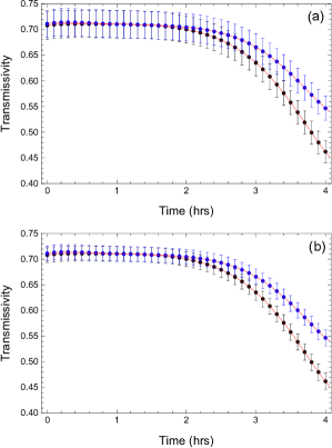
To further explore this capability, let us also study the performance in the early discrimination between different bacteria, starting from the experimental data obtained for E. coli and Salmonella (see Fig. 3). As before the experimental data in absorbance $A$ can be expressed in terms of the transmissivity $\eta=10^{-A}$ and the corresponding growth curves of the two bacteria can be interpolated by two polynomial functions $\eta_{\text{Ecoli}}(t)$ and $\eta_{\text{Salmo}}(t)$. At each reading time $t$, the data points $\{\eta_{k}\}_{k=1}^{N}$ of a theoretical quantum measurement provide an estimator $\hat{\eta}$ of the transmissivity $\eta(t)$. The minimum error $\sigma_{\eta}$ will be given by the QCRB relative to the specific source and the mean total number of photons $\bar{n}_{\text{tot}}$ irradiated over the sample. The numerical performances of coherent states and optimal quantum states are shown in Fig. 8, up to $4$ hours. We can see that, while the quantum source certainly narrows the error bars, the early discrimination between the two bacteria appear to be more difficult than detecting a generic growth with respect to the blank.

Figure 8: Decay of transmissivity due to the growth of E. coli (black points) and Salmonella (blue points) versus time $t$ (hours). The sample is monitored by irradiating a total of $\bar{n}_{\text{tot}}=10^{3}$ mean photons for each reading. Error bars refer to one standard deviation as given by the QCRB. In (a) we consider coherent states as the input source, while in (b) we consider optimal quantum states. The mean decay (red lines) are given by curves $\eta_{\text{Ecoli}}(t)$ and $\eta_{\text{Salmo}}(t)$ that are extrapolated by the experimental data from Fig. 3.

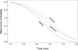
For the null hypothesis $H_{0}$ (growth of Salmonella), the estimator $\hat{\eta}$ is centered around $\eta_{\text{Salmo}}(t)$ according to a Gaussian distribution $p_{0}(\eta)$ with standard deviation $\sigma_{\eta_{\text{Salmo}}(t)}$. For the alternative hypothesis $H_{1}$ (growth of E. coli), the estimator $\hat{\eta}$ will be instead centered around $\eta_{\text{Ecoli}}(t)$ according to a Gaussian distribution $p_{1}(\eta)$ with standard deviation $\sigma_{\eta_{\text{Ecoli}}(t)}$. As before, we consider a decision test with threshold $0\leq\tau\leq 1$: if $\hat{\eta}\geq\tau$ we accept the null hypothesis $H_{0}$, while if $\hat{\eta}<\tau$ we accept the alternative hypothesis $H_{1}$. The associated false-positive $p_{\text{FP}}$ and false-negative $p_{\text{FN}}$ error probabilities are defined as in Eqs. (12) and (13). From these probabilities $p_{\text{FP}}(\tau,t)$ and $p_{\text{FN}}(\tau,t)$, we can construct the mean error probability $p_{\text{mean}}(t):=\min_{\tau}[p_{\text{FP}}(\tau,t)+p_{\text{FN}}(\tau,t)]/2$ for equal priors. We compare this mean error probability assuming coherent state sources, optimal and practical quantum sources irradiating the same mean number of total photons $\bar{n}_{\text{tot}}$ per reading. As depicted in Fig. 9, an optimal quantum source gives a clear advantage in the early discrimination between the two bacteria, even though the advantage seems to be reduced to less than one hour (about 30 minutes). This quantum advantage is further reduced but yet present when considering the practical quantum source (based on $1$ dB squeezed vacuum).

Figure 9: Early symmetric discrimination of E. coli and Salmonella. We plot the mean error probability versus time $t$ (hours) for a coherent-state source (dashed line), an optimal quantum source (solid black line), and a practical quantum source (solid purple line), all irradiating $\bar{n}_{\text{tot}}=10^{3}$ mean total photons per reading. For the practical quantum source, we consider a tensor-product of $1$ dB squeezed vacua, so that we need $N=75113$ probes per reading.

V Conclusion

In this work, we have explored the potentialities of a quantum-enhanced model of spectrophotometer in detecting and tracking bacterial growth in samples. Starting from experimental growth curves of two bacteria, E. coli and Salmonella, we simulate the theoretical performance achievable by a quantum design that is based on an input source, semiclassical or a truly-quantum, combined with an optimal quantum measurement at the output. We first discuss how this device could efficiently work with orders of magnitude fewer photons, also identifying the regime (low concentrations/absorbances) where quantum sources can provide a non-trivial advantage. We have further explored this regime considering tasks of early detection of bacterial growth and early discrimination between two bacterial species. In each case, we have shown that truly-quantum light allows us to improve the detection/discrimination performance with respect to the use of coherent states.

In conclusion, our work contributes to clarify the potentialities of noninvasive quantum sensing techniques for biological and biomedical applications. Further investigations may be aimed at the exploration of similar advantages for other types of bacteria, the explicit design of optimal receivers, and the simultaneous discrimination of multiple ($>2$) species growing within a sample.

Acknowledgments. This work has been sponsored by European Union’s Horizon 2020 Research and Innovation Action under grant agreements No. 745727 (Marie Skłodowska-Curie Global Fellowship “quantum sensing for biology”, QSB) and No. 862644 (“Quantum readout techniques and technologies”, QUARTET). GS and LP would like to thank Janine Maddock, Mattew Chapman and Janet Price for discussions. OL acknowledges expertise gained while working at the Chandra X-ray Center. OL contributed to this work in his own time, not as part of his CXC duties.

Author Contributions. GS and SP conceived the idea, developed the scheme, and proved both the analytical results and the numerical results displayed in the plots. GS and LP performed the experiments with the classical instruments. GS and OL performed the data analysis of the experimental data. SP and GS wrote the manuscripts with edits by SLB.

Methods

Description of the experiments

In the first experiment, we have averaged over a single strain of E. coli MRE600 Meier . The strain was measured while growing in a Luria Bertani (LB) broth at $30^{\circ}$C. In particular, three different colonies of the MRE600 strain were selected from a Petri plate and incubated overnight. Each colony was then re-suspended in 5ml LB and let grow at $30^{\circ}$C overnight. Subsequently, each culture has been diluted 1:100 in new flasks containing fresh LB (a total of 3 flasks), so that the initial optical density (OD) at 600 nm was 0.02 for all of them. The new cultures were incubated at $30^{\circ}$C and the OD was measured at various times with 4 different dilution (1:1; 1:2; 1:5 and 1:10) with a technical replicate for each dilution for a total of $24$ samples. The duration of the experiment was 6 hours and the measurements were performed by using a single-beam spectrophotometer (Ultraspect 2100 pro Amersham Bioscience). The results of the readings were then post-processed Data . During the post-processing analysis, some of the data points were filtered considering the appropriate dilutions and the fact that readings of OD that are greater than $1$ are not reliable. We call OD_d the optical density measured for a 1:$d$ diluted sample. We only accept measured values such that OD${}_{d}<1$. Then, we compute the effective (non-diluted) OD of the sample as $d^{-1}$OD_d which is the quantity plotted in Fig. 1. At each measurement time, the appropriate readings from all the strains were combined to form a single vector of $24$ data points, over which we computed average and standard deviation.

In the second experiment, we have analyzed a strain of E. coli BW25113 Meier and a strain of Salmonella (textitenterica serovar Typhimurium ATCC 14028). LB broth was used again to grow the two species at $30^{\circ}$C. As before, 3 colonies of each species were grown in different test tubes overnight and later diluted (roughly 1:100) in new test tubes with fresh LB in order to have all the cultures at the same starting point (around OD of 0.02 at 600 nm). Each tube was then used to provide 6 samples for a total of 18 samples per species. These 18 samples were transferred to the micro-plate of an automatic spectrophotometer (infinite M200 Pro microplate reader by Tecan). This particular instrument performed readings of the $18$ samples every $30$ minutes for $20$ hours. The contribution of the blank was estimated from $4$ blank samples also measured every $30$ minutes for $20$ hours, for a total of $4\times 40=160$ measurements. The blank contribution to the absorbance was equal to $0.144\pm 0.006$. The results of the readings were then post-processed Data .

V.1 Delta method

In general, consider a sequence of random variables $X_{n}$ converging in distribution to a normal variable $X$ with (finite) mean value $\bar{X}$ and (finite) variance $\mathrm{var}(X)$. Convergence in distribution means that the cumulative function $F_{n}$ of $X_{n}$ converges to the cumulative function $F$ of $X$, pointwise in the entire region where $F$ is continuous. Now take a differentiable function $A(X)$ with non-zero first derivative. Then, the sequence $A(X_{n})$ converges in distribution to a limit variable, which is normal with mean value $A(\bar{X})$ and variance $[A^{\prime}(\bar{X})]^{2}\mathrm{var}(X)$. This is the case when $A(X)=-\log_{10}(X)$ for which we have $[A^{\prime}(\bar{X})]^{2}=[(\mathrm{ln}10)\bar{X}]^{-2}$. For sufficiently large number of probings, we can assume, with good approximation, that the transmissivity $\eta$ is distributed normally around the mean value $\bar{\eta}$ with small standard deviation $\sigma_{\eta}$. Therefore, we can write the first-order approximation $\sigma_{A}\simeq\sigma_{\eta}/(\bar{\eta}\ln 10)$.

Performance of correlated-thermal states

The formulas in the main text refer to single-mode sources. Let us here consider a two-mode source, therefore suitable for a double-beam design. In particular, we consider a two-mode correlated thermal state combined with a practical quantum detection at the output based on photon counting.

Recall that a two-mode correlated thermal state is a zero-mean Gaussian state with covariance matrix RMP

$$\mathbf{V}_{AB}=\left(\begin{array}[c]{cc}a\mathbf{I}&c\mathbf{I}\\ c\mathbf{I}&b\mathbf{I}\end{array}\right),$$ (17)

where $\mathbf{I}=\mathrm{diag}(1,1)$ and

$$a :=\bar{n}+1/2,~{}b:=\bar{n}(x^{-1}-1)+1/2,$$ (18)

$$c :=\sqrt{(1-x)/x}\bar{n}.$$ (19)

Here $\bar{n}$ is the mean number of thermal photons in the mode $A$ irradiated over the sample, while $0<x<1$ is an asymmetry parameter, so that mode $B$ contains $\bar{n}(x^{-1}-1)$ mean thermal photons. We perform photon counting on the output modes $A$ (sent through the sample with transmissivity $\eta$) and $B$ (directly sent to the receiver).

The optimal performance is given by the classical Cramer-Rao bound

$$\sigma_{\eta}^{2}\geq\frac{1}{Nh_{\eta,\bar{n},x}},$$ (20)

where the classical Fisher information $h_{\eta,\bar{n},x}$ is Sped

$$h_{\eta,\bar{n},x}=\frac{\gamma\bar{n}}{\eta},~{}\gamma:=\frac{1+(1-x)\bar{n}x^{-1}}{1+(1-x+x\eta)\bar{n}x^{-1}}\leq 1.$$ (21)

Using Eq. (3), we therefore find

$$\sigma_{A}\gtrsim\frac{1}{\ln 10}\sqrt{\frac{10^{A}}{\gamma\bar{n}_{\text{tot}}}},$$ (22)

where $\gamma=\gamma(x,\bar{n},A)$ by replacing $\eta=10^{-A}$ in Eq. (21). For fixed absorbance $A$ and input energy $\bar{n}$, we can optimize $\sigma_{A}$ over $x$. For large asymmetry $x\rightarrow+\infty$, we get $\gamma\rightarrow 1$, so that Eq. (22) becomes equal to Eq. (6) which is the optimal performance achievable by coherent states (with an optimal quantum measurement).

References

- (1) G. Sezonov, D. Joseleau-Petit, and R. D’Ari, Escherichia coli Physiology in Luria-Bertani Broth, J. Bacteriol. 189, 8746-8749 (2007).
- (2) M. H. Zwietering, I. Jongenburger, F. M. Rombouts, and K. van’t Riet, Modeling of the Bacterial Growth Curve, Appl. Environ. Microbiol. 56, 1875-1881 (1990).
- (3) R. M. Maier, and I. L. Pepper, Chapter 3 - Bacterial Growth, Editor(s): I. L. Pepper, C. P. Gerba, T. J. Gentry, Environmental Microbiology (Third Edition), Academic Press, 2015, pp. 37-56.
- (4) Note that this definition is close to the quantification of loss in decibels, which includes an additional factor , i.e., .
- (5) P. Bouguer, Essai d’optique sur la gradation de la lumière (Jombert, Paris, 1729).
- (6) J. H. Lambert, Photometria sive de mensura et gradibus luminis, colorum et umbrae (sumptibus viduae Eberhardi Klett, January 1760).
- (7) A. Beer, Bestimmung der Absorption des rothen Lichts in farbigen Flüssigkeiten [Determination of the absorption of red light in colored liquids], Annalen der Physik 62, 78-88 (1852).
- (8) J. D. J Ingle, and S. R. Crouch, Spectrochemical Analysis (New Jersey: Prentice Hall, 1988).
- (9) G. Adesso, F. Dell’Anno, S. De Siena, F. Illuminati, and L. A. M. Souza, Optimal estimation of losses at the ultimate quantum limit with non-Gaussian states, Phys. Rev. A 79, 040305(R) (2009).
- (10) D. Braun, G. Adesso, F. Benatti, R. Floreanini, U. Marzolino, M. W. Mitchell, and S. Pirandola, Quantum-enhanced measurements without entanglement, Rev. Mod. Phys. 90, 035006 (2018).
- (11) S. L. Braunstein, and C. M. Caves, Statistical distance and the geometry of quantum states, Phys. Rev. Lett. 72, 3439 (1994).
- (12) J. P. Meier-Kolthoff et al., Complete genome sequence of DSM 30083(T), the type strain (U5/41(T)) of Escherichia coli, and a proposal for delineating subspecies in microbial taxonomy, Standards in genomic sciences 9, 2 (2014).
- (13) B. Gompertz, On the nature of the function expressive of the law of human mortality, and on a new mode of determining the value of life contingencies, Philos. Trans. R. Soc. London 115, 513-585 (1825).
- (14) J. L. Doob, The Limiting Distributions of Certain Statistics, Annals of Mathematical Statistics 6, 160-169 (1935).
- (15) R. Dorfman, A Note on the -Method for Finding Variance, The Biometric Bulletin 1, 129-137 (1938).
- (16) J. M. Ver Hoef, Who invented the delta method?, The American Statistician 66, 124-127 (2012).
- (17) C. Weedbrook, S. Pirandola, R. García-Patrón, N. J. Cerf, T. C. Ralph, J. H. Shapiro, and S. Lloyd, Gaussian Quantum Information, Rev. Mod. Phys. 84, 621 (2012).
- (18) L. Banchi, S. L. Braunstein, and S. Pirandola, Quantum Fidelity for Arbitrary Gaussian States, Phys. Rev. Lett. 115, 260501 (2015).
- (19) A. Monras, and M. G. A. Paris, Optimal Quantum Estimation of Loss in Bosonic Channels, Phys. Rev. Lett. 98, 160401 (2007).
- (20) G. Spedalieri, C. Lupo, S. L. Braunstein, and S. Pirandola, Thermal quantum metrology in memoryless and correlated environments, Quantum Sci. Technol. 4, 015008 (2019).
- (21) M. G. A. Paris, Quantum estimation for quantum technology, Int. J. Quant. Inf. 7, 125-137 (2009).
- (22) M. Hayashi, M., Quantum Information, (Springer Berlin, 2006).
- (23) R. D. Gill, and S. Massar, State estimation for large ensembles, Phys. Rev. A 61, 042312 (1999).
- (24) J. Arnbak, C. S. Jacobsen, R. B. Andrade, X. Guo, J. S. Neergaard-Nielsen, U. L. Andersen, and T. Gehring, Compact, low-threshold squeezed light source, Opt. Express 27, 37877-37885 (2019).
- (25) Data and code for figures are available at the doi: 10.5281/zenodo.4127011.