Dark Radiation from Inflationary Fluctuations

Abstract

Light new vector bosons can be produced gravitationally through quantum fluctuations during inflation; if these particles are feebly coupled and cosmologically metastable, they can account for the observed dark matter abundance. However, in minimal anomaly free $U(1)$ extensions to the Standard Model, these vectors generically decay to neutrinos if at least one neutrino mass eigenstate is sufficiently light. If these decays occur between neutrino decoupling and CMB freeze out, the resulting radiation energy density can contribute to $\Delta N_{\rm eff}$ at levels that can ameliorate the Hubble tension and be discovered with future CMB and relic neutrino detection experiments. Since the additional neutrinos are produced from vector decays after BBN, this scenario predicts $\Delta N_{\rm eff}>0$ at recombination, but $\Delta N_{\rm eff}=0$ during BBN. Furthermore, due to a fortuitous cancellation, the contribution to $\Delta N_{\rm eff}$ is approximately mass independent.

I Introduction

Cosmological inflation elegantly accounts for the observed flatness, isotropy, and homogeneity of the universe. Additionally, the quantum mechanical fluctuations in the inflaton field during inflation generate a nearly scale invariant spectrum of density perturbations that seed the growth of structure and imprint temperature anisotropies onto the cosmic microwave background (CMB) – see Ref. Baumann (2009) for a review.

It is well known that new, feebly coupled particles are produced gravitationally through quantum fluctuations during inflation if their masses are small compared to the inflationary Hubble scale $H_{I}$ Mukhanov et al. (1992); heavier particles can also be produced if the inflaton undergoes rapid oscillations Chung et al. (1998); Kuzmin and Tkachev (1999); Ema et al. (2015, 2016, 2018); Chung et al. (2019) or nontrvially affects the particle’s mass during inflation Fedderke et al. (2015). For light spin-0 particles, these fluctuations yield isocurvature perturbations on large scales, which are tightly constrained by CMB observations Seckel and Turner (1985); Linde (1985) and for spin $\nicefrac{{1}}{{2}}$ fermions, inflationary fluctuations are generically suppressed unless they have non-conformal interactions through higher dimension operators Parker (1968); Adshead and Sfakianakis (2015); Adshead et al. (2018).

It has recently been shown that the gravitational production of spin-1 particles during inflation is sharply peaked at modes that re-enter the horizon after inflation when the Hubble scale equals the vector’s mass, $H=m$ Graham et al. (2016). Such scales are typically much smaller than those probed by CMB experiments, so the isocurvature bounds on this scenario are negligible and this mechanism yields a viable dark matter candidate for

$$m\sim\mu{\rm eV}\left(\frac{10^{14}\,\rm GeV}{H_{I}}\right)^{4}~{}.$$ (1)

Thus, if the vector is decoupled from Standard Model (SM) fields or is sufficiently light ($m\ll 2m_{e}$) and interacts only through a small kinetic mixing, its cosmological metastability is generically realized.

However, if the vector is the gauge boson of a minimal $U(1)$ gauge extension, couplings to neutrinos are required for anomaly cancellation Bauer et al. (2018); the only anomaly free groups with no additional SM charged fermions are

$$~{}~{}U(1)_{B-L},~{}~{}U(1)_{L_{i}-L_{j}},~{}~{}U(1)_{B-3L_{i}},$$ (2)

where $B/L$ is baryon/lepton number, $i,j=e,\mu,\tau$ are lepton flavor indices, and the corresponding gauge bosons in these models couple to at least one neutrino flavor. Thus, unlike kinetically mixed dark photon scenarios, the vector decays in these models can be relatively prompt and have observable cosmological consequences.

In this paper, we consider the fate of light gauge bosons $V$ produced during inflation. We assume these vectors couple feebly to neutrinos and that at least one neutrino mass eigenstate is sufficiently light to allow $V\to\bar{\nu}\nu$ decays. If such decays occur after neutrino decoupling, but before CMB photon decoupling, there is an irreducible contribution to $\Delta N_{\rm eff}$ that is potentially observable with future CMB-S4 experiments Abazajian et al. (2016) and a modified relic neutrino spectrum observable at PTOLEMY McKeen (2019); Baracchini et al. (2018). Furthermore, such a contribution of $\Delta N_{\rm eff}$ can alleviate the discrepancy between early and late time measurements of the Hubble constant (for recent reviews see Valentino et al. (2021); Knox and Millea (2020)).

II Stable Vector Abundance

The general lagrangian during inflation contains

$$\frac{\cal L}{\sqrt{\tilde{g}}}\supset-\frac{1}{4}g^{\mu\kappa}g^{\nu\lambda}F_{\mu\nu}F_{\kappa\lambda}+\frac{m^{2}}{2}g^{\mu\nu}V_{\mu}V_{\nu}~{},$$ (3)

where $V$ is a gauge boson in an FRW metric, $F_{\mu\nu}$ is the corresponding field strength tensor, and $\tilde{g}$ is the metric determinant. If the mass satisfies $0<m\ll H_{I}$ and $V$ is stable, the longitudinal mode is gravitationally produced during inflation and constitutes a present-day dark matter fraction $f^{0}_{V}\equiv\Omega_{V}/\Omega_{\rm dm}$ Graham et al. (2016)

$$f^{0}_{V}\approx\frac{\sqrt{m}H_{I}^{2}}{4\pi^{2}M^{3/2}_{\rm Pl}T_{\rm eq}}\approx 10^{-2}\sqrt{\!\frac{m}{10\,\mu\rm eV}}\left(\frac{H_{I}}{10^{13}\rm\,GeV}\right)^{2}\!\!\!,~{}~{}~{}$$ (4)

where $M_{\rm Pl}=1.22\times 10^{19}$ GeV is the Planck mass and $T_{\rm eq}=0.75$ eV is the temperature of matter-radiation equality, so the energy density at earlier times is

$$\rho_{V}(t)=\rho_{V}^{0}\left(\frac{a(t_{0})}{a(t)}\right)^{3},~{}~{}\rho_{V}^{0}\equiv f^{0}_{V}\,\Omega_{\rm dm}\,\rho_{\rm cr}~{},$$ (5)

where $\Omega_{\rm dm}=0.24$ is the fractional dark matter abundance, $\rho_{\rm cr}=4.1\times 10^{-47}\,\rm GeV^{4}$ is the critical density, $a$ is the FRW scale factor, $t_{0}=13.8$ Gyr, and a $0$ label represents a present day quantity Aghanim et al. (2018); Kolb and Turner (1990). For stable vectors, Eq. (5) is valid for $t>t_{\star}=(2m)^{-1}$, the horizon re-entry time corresponding to $H=m$ and temperature

$$T_{\star}=\sqrt{\frac{mM_{\rm Pl}}{1.66\,\sqrt{g_{\star}}}}\approx 85\,{\rm GeV}\left(\frac{100}{g_{\star}}\right)^{1/4}\!\!\left(\frac{m}{10\,\mu\rm eV}\right)^{1/2}\!\!\!\!\!\!,~{}~{}~{}$$ (6)

where $g_{\star}$ is the effective number of relativistic SM species in equilibrium. Note that because the $V$ power spectrum is dominated by momentum modes that re-enter the horizon when $H\sim m$, the $V$ population is nonrelativistic for all times $t>t_{\star}$.

III Adding Decays to Neutrinos

Since abelian gauge extensions to the SM generically feature neutrino couplings, we add the representative interaction

$${\cal L}\supset gV_{\mu}\bar{\nu}_{i}\gamma^{\mu}\nu_{i}~{},$$ (7)

to Eq. (3), where $g\ll 1$ is a gauge coupling and $i$ is a lepton family index. In the massless neutrino limit, the partial width to a single flavor is Escudero et al. (2019)

$$\Gamma(V\to\bar{\nu}_{i}\nu_{i})=\frac{g^{2}m}{24\pi}~{},$$ (8)

the total width $\Gamma_{V}$ is the sum of all allowed channels and $\tau_{V}=\Gamma_{V}^{-1}$ is the $V$ lifetime. We note that a single massless neutrino eigenstate is empirically viable Tanabashi et al. (2018); De Salas et al. (2018), so, in principle, at least one decay channel is allowed for all vector masses.

Unlike in Ref Graham et al. (2016), here the vector is unstable and $V\to\bar{\nu}\nu$ decays deplete the initial population, so Eq. (5) is only useful for establishing the initial condition for $\rho_{V}$ at $t=t_{\star}$. Accounting for decays to neutrinos, the $V$ population can now be written

$$\rho_{V}(t)=\rho^{0}_{V}\left(\frac{a(t_{0})}{a(t)}\right)^{3}e^{-\Gamma_{V}(t-t_{\star})}~{},$$ (9)

and the energy density of the modified neutrino population $\delta\rho_{\nu}$ evolves according to

$$\delta\dot{\rho}_{\nu}+4H\delta\rho_{\nu}=\Gamma_{V}\rho_{V}~{},$$ (10)

which can be integrated to yield

$$\delta\rho_{\nu}(t)=\frac{\Gamma_{V}}{a(t)^{4}}\int_{t_{\nu}}^{t}dt^{\prime}a(t^{\prime})^{4}\rho_{V}(t^{\prime})~{},$$ (11)

where $a$ is the FRW scale factor and $t_{\nu}\sim$ 1 sec is the time of neutrino decoupling; we only keep contributions for $t>t_{\nu}$ because neutrinos injected before $t_{\nu}$ thermalize with the radiation bath and do not contribute to dark radiation. Similarly, $V$ that decay after CMB decoupling will not contribute to $\Delta N_{\rm eff}$, but will increase the dark matter density during recombination. In Fig. 3 we show a representative solution of Eq. (10) plotted as a fraction of the total energy density.

In terms of the equivalent number of SM neutrinos $\Delta N_{\rm eff}$, this additional radiation from $\delta\rho_{\nu}$ predicts

$$\Delta N_{\rm eff}\equiv\frac{8}{7}\left(\frac{11}{4}\right)^{4/3}\frac{\delta\rho_{\nu}}{\rho_{\gamma}}\,\biggr{|}_{T_{\rm cmb}},$$ (12)

where $\rho_{\gamma}=\pi^{2}T^{4}/15$ and the contribution is evaluated at the temperature of photon decoupling, $T_{\rm cmb}\approx 0.2$ eV; this sets the upper integration range in Eq. (11) since $V$ decays after last scattering do not contribute to dark radiation in the CMB data set.

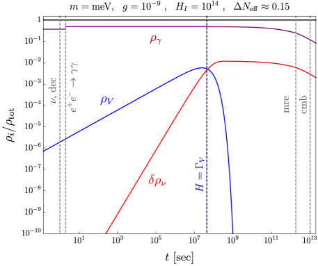
Figure 1: Time dependent energy fractions $\rho_{i}/\rho_{\rm tot}$ for a benchmark choice of model inputs. Here $\rho_{\rm tot}=3M_{\rm Pl}^{2}H^{2}/8\pi$ is the total energy density of the universe and we show $\rho_{V}$, the density of vectors from inflationary production, $\delta\rho_{\nu}$ the additional neutrino density from $V\to\bar{\nu}\nu$ decays assuming a single neutrino flavor. From left to right, the vertical dashed lines mark neutrino decoupling, matter radiation equality, and CMB decoupling. Note that in Eq. (18), the number density of the neutrino population from $V$ decays might exceed that of the relic neutrino background, but as seen here, the energy density remains small for empirically viable values of $\Delta N_{\rm eff}$.

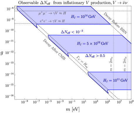
Figure 2: Parameter space that yields observable levels of dark radiation from a population of gravitationally produced vectors that decay via $\to\bar{\nu}\nu$ after neutrino decoupling but before recombination. Horizontal blue shaded bands represents regions where $10^{-2}<\Delta N_{\rm eff}<0.5$ for representative choices of the inflationary Hubble scale $H_{I}$; for each choice, the parameter space below the bottom boundary predicts $\Delta N_{\rm eff}>0.5$, which is excluded assuming otherwise standard cosmological assumptions Blinov et al. (2019); Depta et al. (2019); Aghanim et al. (2018). Above the horizontal dotted lines, $V$ thermalizes with the SM, yielding $\Delta N_{\rm eff}\approx 2.5$ Blinov et al. (2019), which is excluded if $V$ couples to $e$ or $\mu$. The vertical dotted lines mark $m=2m_{e,\mu}$ where $V\to e^{+}e^{-}$ and $V\to\mu^{+}\mu^{-}$ decays are kinematically allowed. Most models in Eq. (2) feature $V$-$e$ couplings, so for $m>2m_{e}$ the $\Delta N_{\rm eff}\approx 0$ as $V\to e^{+}e^{-}$ decays heat photons to compensate for $V\to\bar{\nu}\nu$ decays, which heat neutrinos.

For the full parameter space, $\Delta N_{\rm eff}$ in Eq. (12) must be computed numerically by solving Eq. (11). However, if $V$ decays between $T_{\nu,\rm dec}$ and $T_{\rm eq}$, the decay temperature can be written

$$T_{\rm decay}\approx\sqrt{\frac{g^{2}mM_{\rm Pl}}{40\pi\sqrt{g_{\star}}}}\approx 100\,{\rm eV}\!\left(\frac{g}{10^{-8}}\right)\!\left(\frac{m}{10^{-5}\,\rm eV}\right)^{1/2}\!\!\!\!\!,~{}~{}~{}~{}~{}~{}$$ (13)

where $g_{\star}\approx 3.36$ in our temperature range of interest between decoupling and recombination. Assuming instantaneous $V\to\bar{\nu}\nu$ decay and approximating $\delta\rho_{\nu}\approx\rho_{V}(T_{\rm decay})$ using Eq. (5), Eq. (12) becomes

$$\Delta N_{\rm eff} \approx \frac{30}{7\pi^{4}}\left(\frac{11}{4}\right)^{4/3}\frac{\Omega_{\rm dm}\,\rho_{\rm cr}\sqrt{m}H_{I}^{2}}{M^{3/2}_{\rm Pl}T_{0}^{3}T_{\rm eq}T_{\rm decay}}$$ (14)

$$\approx 10^{-2}\left(\frac{H_{I}}{10^{14}\,\rm GeV}\right)^{2}\left(\frac{10^{-8}}{g}\right)~{},~{}~{}$$

where the vector mass has canceled.

In Fig. 2 we show $\Delta N_{\rm eff}$ predictions for the inflationary vector population where we compute $\delta\rho_{\nu}$ numerically using Eq. (11). The blue horizontal bands represent the currently viable $10^{-2}\leq\Delta N_{\rm eff}<0.5$ range that is within the reach of CMB-S4 predictions Abazajian et al. (2016). Note that current BBN bound $\Delta N_{\rm eff}<0.5$ Blinov et al. (2019) is less stringent than the CMB and large scale structure bound $\Delta N_{\rm eff}<0.28$ Aghanim et al. (2018), but the BBN limit is less model dependent because it is not as sensitive to the choice of cosmological model. However, despite the nominal choice of $\Delta N_{\rm eff}<0.5$ as our conservative exclusion benchmark, this scenario is not directly constrained by the BBN measurement of $\Delta N_{\rm eff}$ since the additional neutrinos from $V$ decays do not appear until after BBN.

The area in between the dashed diagonal bands represent parameter space for which $V\to\bar{\nu}\nu$ decays occur between neutrino and CMB decoupling; decays outside this band do not contribute to $\Delta N_{\rm eff}.$ The vertical lines at $m=2m_{e},2m_{\mu}$ represent regions where the $\Delta N_{\rm eff}$ prediction here does not apply if $V$ couples to electrons or muons; in such models, $V$ decays to charged particles after neutrino decoupling will heat photons and thereby reduce $\Delta N_{\rm eff}$ relative to Eq. (14).

We note for completeness that there is also a possible contribution to $\Delta N_{\rm eff}$ from the $V$ population itself if an appreciable fraction of the $\rho_{V}$ redshifts like radiation at recombination. Since inflationary $V$ production is sharply peaked around modes that enter the horizon at $H\sim m$, from Eq. (6) only masses below $m\lesssim 10^{-30}$ eV will be quasi relativistic around $T_{\rm cmb}$. However, from Eq. (4) such small masses yield negligible inflationary production for all $H_{I}\lesssim 10^{14}$ GeV allowed by CMB limits on tensor modes Aghanim et al. (2018); Marsh (2016), so we can safely neglect this contribution.

IV Interactions with the SM Plasma

The above discussion assumes that the early universe $V$ population arises entirely to inflationary production and is unaffected by the SM radiation bath. However, for any value of the gauge coupling, there is irreducible sub-Hubble “freeze-in” production of additional $V$ Dodelson and Widrow (1994); Hall et al. (2010); Fradette et al. (2014); Escudero et al. (2019) and, if the coupling is sufficiently large, the $V$ population can thermalize with the SM plasma; which yields additional contributions to $\Delta N_{\rm eff}$.

• Inverse Decays
  Independently of any other assumptions about ultralight $V$ partilces beyond their coupling to neutrinos, there is a bound on thermalizing with the SM plasma via population via $\bar{\nu}\nu\leftrightarrow V$ decays and inverse decays. If thermalization occurs before neutrino decoupling, this scenario predicts $\Delta N_{\rm eff}\approx 2.5$, so avoiding this fate requires

  $$~{}~{}~{}~{}~{}~{}\frac{\Gamma_{\bar{\nu}\nu\to V}}{H}\!\sim\!\frac{g^{2}m^{2}M_{\rm Pl}}{T_{\nu,\rm dec}^{3}}\!\ll\!1\!\implies\!g\lesssim 10^{-5}\!\left(\frac{\rm eV}{m}\right)\!,~{}~{}~{}$$ (15)

  where $T_{\nu,\rm dec}\sim$ MeV is the temperature of neutrino decoupling via the SM weak interactions. If, instead, thermalization occurs between $T_{\nu,\rm dec}$ and $T_{\rm cmb}$ as in Ref. Berlin and Blinov (2018), then $\Delta N_{\rm eff}\sim 0.2$ independently of mass and coupling Escudero et al. (2019). Since this contribution is fixed only by the neutrino coupling, it must be added to the component from the inflationary population.

• Production From Charged Particles
  If $V$ also couples to charged fermion $f$, dangerous $\bar{f}f\to\gamma V$ and $f\gamma\to fV$ processes can thermalize $V$ with the SM radiation bath, thereby yielding $\Delta N_{\rm eff}\approx 2.5$, which is excluded by both BBN and CMB observables Escudero et al. (2019); Blinov et al. (2019); Depta et al. (2019); Aghanim et al. (2018). The $V$ production rate can be estimated as $\Gamma_{\bar{f}f\to V\gamma}\sim\Gamma_{f\gamma\to fV}\sim\alpha g^{2}T/4\pi$, so these processes grow relative to Hubble until $T\sim m_{f}$, when they become Boltzmann suppressed. Ensuring that the maximum rate not exceed Hubble expansion requires

  $$g\lesssim\sqrt{\frac{4\pi\sqrt{g_{\star}}m_{f}}{\alpha M_{\rm Pl}}}=\begin{cases}5\times 10^{-10}~{},&f=e\\ 7\times 10^{-9}~{},&f=\mu\end{cases},$$ (16)

  where $g_{\star}$ is evaluated at $T=m_{e},m_{\mu}$, respectively. The stronger electron based bound here applies to most anomaly free $U(1)$ extensions – including gauged $B-L$, $B-3L_{e}$, $L_{e}-L_{\mu}$, $L_{e}-L_{\tau}$ – as they all require $V$ to couple to electrons for anomaly cancellation Bauer et al. (2018); the main outlier is gauged $L_{\mu}-L_{\tau}$ for which muon induced thermalization is the dominant process at low temperatures Escudero et al. (2019), so the bound is somewhat weaker. Both of the requirements in Eq. (16) are presented in as dotted horizontal black curves in Fig. 2 and the parameter space above these regions is excluded if the model in question features the corresponding $e$ or $\mu$ coupling.

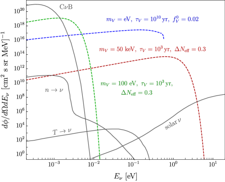
Figure 3: Present day neutrino flux spectra from $V\to\bar{\nu}\nu$ decays for representative benchmark points (dashed). Also shown are spectra from the C$\nu$B, primordial neutron decays during BBN ($n\to\nu$), tritium decays during BBN $(T\to\nu)$, and solar neutrinos McKeen (2019). From Eq. (21), is clear that the early decaying parameter points (green and red) only yield appreciable ($\gtrsim$ few) events at PTOLEMY for lower values of $m_{V}$, which are difficult to distinguish from the C$\nu$B spectrum, but might be detected as an enhancement over the Standard Model signal rate. As the mass is increased, the spectrum gets harder, but the rate becomes unobservable with a feasible exposure; for the 50 keV benchmark, we find $R\sim 10^{-3}$ events/yr at PTOLEMY. For later decaying particles (blue dashed curve) the rate and spectrum can be favorable, but there is no contribution to $\Delta N_{\rm eff}.$

We emphasize that the parameter space shown in Fig. 2 is extremely weakly coupled, such that there is no danger of the inflationary $V$ population thermalizing with the SM plasma, or of any appreciable contributions from SM processes that produce additional $V$ particles via inverse decays or SM scattering reactions. For a careful study of such processes in the context of the models studied here, see Escudero et al. (2019) which identifies the parameter space where freeze in production via inverse decays contributes to cosmological observables including $\Delta N_{\rm eff}$.

V Present Day Neutrino Flux

In this section we review the results of Ref. McKeen (2019), adapted to the case of inflationary vector production. The neutrinos in our scenario arises from $V$ decays and if the entire population decays in the early universe, the present day number density is

$$\delta n_{\nu}(t_{0})=\frac{f_{V}^{0}\,\Omega_{\rm dm}\,\rho_{\rm cr}}{m_{V}}\approx 130\,{\rm cm^{-3}}\,\left(\frac{f_{V}^{0}}{0.05}\right)\left(\frac{\rm eV}{m}\right)\!.~{}~{}~{}$$ (17)

If these decays occur between neutrino decoupling and recombination, Eq. (17) can be rewritten McKeen (2019)

$$\delta n_{\nu}(t_{0})\approx 10^{3}{\rm cm}^{-3}\left(\frac{\Delta N_{\rm eff}}{0.28}\right)\left(\frac{\rm eV}{m}\right)\sqrt{\frac{10^{3}\,\rm yr}{\tau_{V}}}.~{}~{}~{}~{}$$ (18)

Although the number density of additional neutrinos in Eq. (18) can exceed the $\sim 300{\rm\,cm}^{-3}$ number density of the cosmic neutrino background (C$\nu$B) as predicted in the Standard Model, as long as the corresponding value of $\Delta N_{\rm eff}$ satisfies observational bounds, the energy density of this population is always subdominant and remains empirically viable.

For some parameter choices, this additional neutrino population may be observable with the PTOLEMY experiment using inverse beta decay reactions from captured relic neutrinos Baracchini et al. (2018). Assuming a detector target mass of $M_{T}$, electron neutrino fraction $f_{\nu_{e}}$, neutrino capture cross section on tritium $\sigma=3.83\times 10^{-45}$ cm², and the excess neutrino density from Eq. (18), the signal rate is estimated to be McKeen (2019)

$$R\approx\frac{5}{\rm yr}\left(\frac{M_{T}}{100\,\rm g}\right)\left(\frac{f_{\nu_{e}}}{0.5}\right)\left(\frac{f_{V}^{0}}{0.05}\right)\left(\frac{\rm eV}{m_{V}}\right)~{},$$ (19)

which only assumes that the $V$ decay after decoupling. However, for $V$ that also decay before recombination, the fraction satisfies McKeen (2019)

$$f_{V}^{0}\approx 0.42\left(\frac{\Delta N_{\rm eff}}{0.3}\right)\left(\frac{10^{3}\,\rm yr}{\tau_{V}}\right),$$ (20)

so the rate for early decaying $V$ can be written

$$R\approx\frac{10}{\rm yr}\left(\frac{M_{T}}{100\,\rm g}\right)\left(\frac{f_{\nu_{e}}}{0.5}\right)\left(\frac{\Delta N_{\rm eff}}{0.3}\right)\left(\frac{\rm 10\,eV}{m_{V}}\right)~{},$$ (21)

which may be detectable with a year of exposure at PTOLEMY, whose projected C$\nu$B sensitivity is at the $\sim 10$ event level. Note that there is general tension between having an appreciable $\Delta N_{\rm eff}$ signal and having a distinguishable neutrino spectrum with a detectable PTOLEMY rate.

To see this, note that the late time flux of neutrinos from $V$ decays is

$$\frac{d\phi}{d\Omega dE_{\nu}}=\frac{f_{V}^{0}\,\Omega_{\rm dm}\,\rho_{\rm cr}}{2\pi m_{V}E_{\nu}}\frac{\Gamma_{V}\,e^{-\Gamma_{V}(t-t_{\star})}}{H(z_{c})}\Theta(t-t_{\nu,\rm dec}),~{}~{}~{}$$ (22)

where $E_{\nu}$ is the observed energy of a present day neutrino emitted at redshift $z$ with energy $E_{\nu}(1+z)=m_{V}/2$, $H(z)=H_{0}\sqrt{\Omega_{\Lambda}+\Omega_{m}(1+z)^{3}+\Omega_{r}(1+z)^{4}}$ is the Hubble rate, $H_{0}=67$ km/sec/Mpc Aghanim et al. (2018), and $z_{c}=[m_{V}/(2E_{\nu})]-1$. The theta function ensures that decays before neutrino decoupling do not contribute to the flux; this population will thermalize with C$\nu$B. In Fig. 3 we show representative flux spectra for both early ($t_{\nu,\rm dec}<\tau_{V}<t_{\rm cmb})$ and late time $(\tau_{V}>t_{\rm cmb})$ decaying populations. From Eq. (21), early decaying $V$ with low $\sim$ few eV masses can yield appreciable PTOLEMY signal rates, but as we see in these spectra, the fluxes similar to the C$\nu$ unless $m_{V}$ much greater, which trades off against the overall rate as $R\propto m_{V}^{-1}$. It is possible to get an appreciable PTOLEMY flux for a low mass particle, but obtaining a distinctive spectral shape requires late time decays, which do not affect $\Delta N_{\rm eff}$.

VI Conclusion

In this paper we have studied the fate of massive vector particles produced gravitationally from inflationary fluctuations. If these vectors only interact with the SM via kinetic mixing, for $m<2m_{e}$, the only allowed decay is $V\to 3\gamma$ which is sharply suppressed, so $V$ is generically metastable can serve dark matter candidate Graham et al. (2016). However, if the vector arises in well motivated, minimal $U(1)$ gauge extensions from Eq. (2), it must couple to neutrinos, so if at least one neutrino mass eigenstate is sufficiently light, $V\to\bar{\nu}\nu$ decays can efficiently deplete this inflationary population and increase the relic neutrino densty, thereby predicting $\Delta N_{\rm eff}\neq 0$. For certain regions of parameter space, the same neutrino population may be observable at late times with the PTOLEMY experiment; for long lived vectors that decay after recombination, it is also possible to obtain an appreciable PTOLEMY signal even though $\Delta N_{\rm eff}=0$.

Intriguingly. due to a cancellation, this contribution depends only on $H_{I}$ and $g$ as long as the $V$ lifetime falls within this time window. For a wide range of model parameters, the $\Delta N_{\rm eff}$ prediction in these scenarios is within reach of CMB-S4 projections Abazajian et al. (2016). We note that, outside of the narrow parameter region where 50 keV $\lesssim T_{\rm decay}\lesssim$MeV, this scenario predicts $\Delta N_{\rm eff}\neq 0$ only in CMB data because nearly all of the $V$ decays occur after BBN has completed; decays before BBN thermalize with the SM, so $T_{\nu}/T_{\gamma}$ does not deviate from the SM prediction. However, for parameter space in this decay occurs after recombination, the resulting neutrino population may be observable directly at PTOLEMY McKeen (2019); Baracchini et al. (2018).

Furthermore, since the mechanism studied here is sensitive to the Hubble scale during inflation, future measurements of inflationary B-modes at CMB-S4 experiments will have important implications for this class of scenarios. The forecasted sensitivity to the scalar-to-tensor ratio $r\sim 10^{-3}$ implies a sensitivity to $H_{I}\sim 10^{12}$ GeV Collaboration (2020), which yields observable $\Delta N_{\rm eff}$ from $V$ decays in the upper half of Fig. 2.

Finally, it has been shown that contributions to $\Delta N_{\rm eff}\sim 0.5$ may play an important role in alleviating the discrepancy between early and late time determinations of the Hubble tension Valentino et al. (2021); Knox and Millea (2020). Although models with nonzero $\Delta N_{\rm eff}$ do not completely eliminate the tension, it is intriguing that the contributions required to reduce its statistical signficance are readily accommodated in the parameter space studied in this class of models.

Acknowledgments: We thank Asher Berlin, Nikita Blinov, Dan Hooper, Kevin Kelly, Rocky Kolb, and David McKeen for helpful conversations. This manuscript has been authored by Fermi Research Alliance, LLC under Contract No. DE-AC02-07CH11359 with the U.S. Department of Energy, Office of High Energy Physics.

References

- Baumann (2009) D. Baumann, “Tasi lectures on inflation,” (2009), arXiv:0907.5424 [hep-th] .
- Mukhanov et al. (1992) V. F. Mukhanov, H. Feldman, and R. H. Brandenberger, Phys. Rept. 215, 203 (1992).
- Chung et al. (1998) D. J. Chung, E. W. Kolb, and A. Riotto, Phys. Rev. D 59, 023501 (1998), arXiv:hep-ph/9802238 .
- Kuzmin and Tkachev (1999) V. Kuzmin and I. Tkachev, Phys. Rev. D 59, 123006 (1999), arXiv:hep-ph/9809547 .
- Ema et al. (2015) Y. Ema, R. Jinno, K. Mukaida, and K. Nakayama, JCAP 05, 038 (2015), arXiv:1502.02475 [hep-ph] .
- Ema et al. (2016) Y. Ema, R. Jinno, K. Mukaida, and K. Nakayama, Phys. Rev. D 94, 063517 (2016), arXiv:1604.08898 [hep-ph] .
- Ema et al. (2018) Y. Ema, K. Nakayama, and Y. Tang, JHEP 09, 135 (2018), arXiv:1804.07471 [hep-ph] .
- Chung et al. (2019) D. J. Chung, E. W. Kolb, and A. J. Long, JHEP 01, 189 (2019), arXiv:1812.00211 [hep-ph] .
- Fedderke et al. (2015) M. A. Fedderke, E. W. Kolb, and M. Wyman, Phys. Rev. D 91, 063505 (2015), arXiv:1409.1584 [astro-ph.CO] .
- Seckel and Turner (1985) D. Seckel and M. S. Turner, Phys. Rev. D 32, 3178 (1985).
- Linde (1985) A. D. Linde, Phys. Lett. B 158, 375 (1985).
- Parker (1968) L. Parker, Phys. Rev. Lett. 21, 562 (1968).
- Adshead and Sfakianakis (2015) P. Adshead and E. I. Sfakianakis, JCAP 11, 021 (2015), arXiv:1508.00891 [hep-ph] .
- Adshead et al. (2018) P. Adshead, L. Pearce, M. Peloso, M. A. Roberts, and L. Sorbo, JCAP 06, 020 (2018), arXiv:1803.04501 [astro-ph.CO] .
- Graham et al. (2016) P. W. Graham, J. Mardon, and S. Rajendran, Phys. Rev. D 93, 103520 (2016), arXiv:1504.02102 [hep-ph] .
- Pospelov et al. (2008) M. Pospelov, A. Ritz, and M. B. Voloshin, Phys. Rev. D 78, 115012 (2008), arXiv:0807.3279 [hep-ph] .
- McDermott et al. (2018) S. D. McDermott, H. H. Patel, and H. Ramani, Phys. Rev. D 97, 073005 (2018), arXiv:1705.00619 [hep-ph] .
- Hoenig et al. (2014) I. Hoenig, G. Samach, and D. Tucker-Smith, Phys. Rev. D 90, 075016 (2014), arXiv:1408.1075 [hep-ph] .
- Bauer et al. (2018) M. Bauer, P. Foldenauer, and J. Jaeckel, (2018), arXiv:1803.05466 [hep-ph] .
- Abazajian et al. (2016) K. N. Abazajian et al. (CMB-S4), (2016), arXiv:1610.02743 [astro-ph.CO] .
- McKeen (2019) D. McKeen, Phys. Rev. D 100, 015028 (2019), arXiv:1812.08178 [hep-ph] .
- Baracchini et al. (2018) E. Baracchini et al. (PTOLEMY), (2018), arXiv:1808.01892 [physics.ins-det] .
- Valentino et al. (2021) E. D. Valentino, O. Mena, S. Pan, L. Visinelli, W. Yang, A. Melchiorri, D. F. Mota, A. G. Riess, and J. Silk, “In the realm of the hubble tension a review of solutions,” (2021), arXiv:2103.01183 [astro-ph.CO] .
- Knox and Millea (2020) L. Knox and M. Millea, Physical Review D 101 (2020), 10.1103/physrevd.101.043533.
- Aghanim et al. (2018) N. Aghanim et al. (Planck), (2018), arXiv:1807.06209 [astro-ph.CO] .
- Kolb and Turner (1990) E. W. Kolb and M. S. Turner, Front. Phys. 69, 1 (1990).
- Escudero et al. (2019) M. Escudero, D. Hooper, G. Krnjaic, and M. Pierre, (2019), arXiv:1901.02010 [hep-ph] .
- Tanabashi et al. (2018) M. Tanabashi et al. (Particle Data Group), Phys. Rev. D 98, 030001 (2018).
- De Salas et al. (2018) P. De Salas, S. Gariazzo, O. Mena, C. Ternes, and M. Tórtola, Front. Astron. Space Sci. 5, 36 (2018), arXiv:1806.11051 [hep-ph] .
- Blinov et al. (2019) N. Blinov, K. J. Kelly, G. Z. Krnjaic, and S. D. McDermott, Phys. Rev. Lett. 123, 191102 (2019), arXiv:1905.02727 [astro-ph.CO] .
- Marsh (2016) D. J. Marsh, Physics Reports 643, 1–79 (2016).
- Depta et al. (2019) P. F. Depta, M. Hufnagel, K. Schmidt-Hoberg, and S. Wild, JCAP 04, 029 (2019), arXiv:1901.06944 [hep-ph] .
- Dodelson and Widrow (1994) S. Dodelson and L. M. Widrow, Phys. Rev. Lett. 72, 17 (1994), arXiv:hep-ph/9303287 .
- Hall et al. (2010) L. J. Hall, K. Jedamzik, J. March-Russell, and S. M. West, JHEP 03, 080 (2010), arXiv:0911.1120 [hep-ph] .
- Fradette et al. (2014) A. Fradette, M. Pospelov, J. Pradler, and A. Ritz, Phys. Rev. D 90, 035022 (2014), arXiv:1407.0993 [hep-ph] .
- Berlin and Blinov (2018) A. Berlin and N. Blinov, Phys. Rev. Lett. 120, 021801 (2018), arXiv:1706.07046 [hep-ph] .
- Collaboration (2020) S. Collaboration, “Cmb-s4: Forecasting constraints on primordial gravitational waves,” (2020), arXiv:2008.12619 [astro-ph.CO] .
- Vattis et al. (2019) K. Vattis, S. M. Koushiappas, and A. Loeb, Phys. Rev. D 99, 121302 (2019), arXiv:1903.06220 [astro-ph.CO] .
- Anchordoqui et al. (2015) L. A. Anchordoqui, V. Barger, H. Goldberg, X. Huang, D. Marfatia, L. H. M. da Silva, and T. J. Weiler, Phys. Rev. D 92, 061301 (2015), [Erratum: Phys.Rev.D 94, 069901 (2016)], arXiv:1506.08788 [hep-ph] .
- Pandey et al. (2019) K. L. Pandey, T. Karwal, and S. Das, (2019), arXiv:1902.10636 [astro-ph.CO] .
- Bringmann et al. (2018) T. Bringmann, F. Kahlhoefer, K. Schmidt-Hoberg, and P. Walia, Phys. Rev. D 98, 023543 (2018), arXiv:1803.03644 [astro-ph.CO] .
- Blinov et al. (2020) N. Blinov, C. Keith, and D. Hooper, JCAP 06, 005 (2020), arXiv:2004.06114 [astro-ph.CO] .
- Clark et al. (2020) S. J. Clark, K. Vattis, and S. M. Koushiappas, (2020), arXiv:2006.03678 [astro-ph.CO] .