Surface cluster algebra expansion formulae via loop graphs

Abstract

In 2011 Musiker, Schiffler and Williams obtained expansion formulae for cluster algebras from orientable surfaces [13]. For singly and doubly notched arcs these formulae required the notion of $\gamma$-symmetric perfect matchings and $\gamma$-compatible pairs of $\gamma$-symmetric perfect matchings, respectively. We simplify and unify these approaches by considering good matchings of loop graphs.

1 Introduction

Fomin and Zelevinsky’s cluster algebras are a particular class of commutative algebras whose generators, cluster variables, are obtained iteratively from an initial collection of (algebraically independent) variables. These cluster variables have some seemingly miraculous properties; even though they are defined recursively as rational functions, surprisingly, they are always Laurent polynomials in the initial variables [6]. In the context of cluster algebras from triangulated surfaces [5], a setting in which cluster variables correspond to tagged arcs on the surfaces, Musiker, Schiffler, Williams significantly strengthened this result. Namely, they showed the coefficients of these Laurent polynomials are always non-negative [13] – a particularly elusive conjecture at the time. Their beautiful result established a remarkable connection between monomials of the Laurent polynomial and perfect matchings of snake graphs. For plain arcs this connection may be thought of as a perfect fit, as there is a bijection between the monomials and the collection of all perfect matchings of the associated snake graph (with respect to an initial ideal triangulation). However, for a general tagged arc this correspondence is somehow lost; one must consider much larger graphs and restrict attention to the so called ‘$\gamma$-symmetric’ perfect matchings’ or ‘$\gamma$-compatible pairs’ of ‘$\gamma$-symmetric’ perfect matchings.

In this paper, in an effort to find an optimal framework for all tagged arcs, we introduce the notion of loop graphs. Roughly speaking this is the result of gluing the end(s) of a snake graph to an existing tile(s). The following theorem shows that good matchings of loop graphs effectively describe the cluster variable expansion of any tagged arc, with respect to any tagged triangulation.

Main Theorem (Theorem 5.7). Let $(S,M)$ be a bordered surface. Let $T^{\circ}$ be an ideal triangulation with corresponding tagged triangulation $T=\iota(T^{\circ})$. Let $\mathcal{A}$ be the associated cluster algebra with principal coefficients with respect to $\Sigma_{T}=(\mathbf{x}_{T},\mathbf{y}_{T},B_{T})$. Suppose $\gamma$ is a tagged arc whose underlying plain arc $\gamma^{\circ}$ is not in $T$, and suppose that $\gamma$ is not notched at any puncture enclosed by a self-folded triangle in $T$ (for technical reasons, if $\gamma$ is doubly notched then we also assume $(S,M)$ is not twice-punctured and closed). Then the Laurent expansion of $x_{\gamma}\in\mathcal{A}$ with respect to $\Sigma_{T}$ is given by:

$$x_{\gamma}=\frac{1}{cross(\gamma,T^{\circ})}\sum_{P}x(P)y(P).$$ (1)

where the sum is taken over all good matchings $P$ of the loop graph $\mathcal{G}_{\gamma,T}$.

We believe the above result will be particularly useful in obtaining skein relations between (generalised) tagged arcs and closed curves on $(S,M)$. As a direct consequence one could then use this to obtain bases for all (full rank) cluster algebras arising from surfaces [Appendix A, [14]].

At first glance the conditions imposed on the Main Theorem may seem quite restrictive. However, we will now explain that the only real restriction comes from the exclusion of doubly notched arcs on twice punctured closed surfaces.

The general case is wishing to write a cluster variable $x_{\gamma}$ with respect to a tagged triangulation $T$, where $\gamma$ is a tagged arc. That being said, this can always be reduced to the case where $T=\iota(T^{\circ})$ and $\gamma$ is not notched inside a self-folded triangle in $T^{\circ}$ by the following symmetry. Let $\gamma$ be a tagged arc and let $\gamma^{\prime}$ be the tagged arc obtained from reversing the tagging of $\gamma$ at each endpoint incident to a puncture. Similarly, let $T$ be a tagged triangulation and let $T^{\prime}$ be the tagged triangulation obtained from reversing the tagging of $T$ at each puncture. Then the function $x_{\gamma}$ written with respect to $T$ is precisely the function $x_{\gamma^{\prime}}$ written with respect to $T^{\prime}$ (this is easily verified directly from the definitions given in Section 2.2).
Note that the Main Theorem also demands that the underlying plain arc $\gamma^{\circ}$ is not in $T$. Nevertheless, a (positive) Laurent expansion may still be obtained from equation (1) if $\gamma^{\circ}\in T$ by the following two approaches. If $\gamma$ is a singly notched arc at a puncture $p$ then we may use the equality $x_{\ell_{p}}=x_{\gamma}x_{\gamma^{\circ}}$ and write $x_{\gamma}$ using equation (1) applied to the arc $\ell_{p}$. If $\gamma$ is doubly notched then a formula is obtained by considering the expansion $x_{\gamma}$ of $\gamma$ with respect to $\mu_{\gamma^{\circ}}(T)$, and showing that $x_{\gamma^{\circ}}$ is a factor of this expression – this property is easily observed directly from the loop graph $\mathcal{G}_{\gamma,\mu_{\gamma^{\circ}}(T)}$.
Finally, regarding the choice of coefficients, by the ‘separation of additions’ formula of Fomin and Zelevinsky [7], it is enough to consider only principal coefficients. Indeed, if $z$ is a cluster variable in a cluster algebra (with any choice of coefficients), their result states $z$ is obtained by a certain specialisation (and rescaling) of the corresponding cluster variable in the cluster algebra with principal coefficients.
Therefore, as in the work of Musiker, Schiffler, Williams [13], the only case for which the Main Theorem does not produce an explicit Laurent expansion is when $\gamma$ is a doubly notched arc on a twice punctured closed surface, and $T$ is an ideal triangulation without a self-folded triangle (or equivalently, $\gamma$ is a plain arc and $T$ is a tagged triangulation for which all endpoints of arcs are notched). Note that by the groundbreaking works of Gross, Hacking, Keel, Kontsevich [9], or Lee, Schiffler [11], the Laurent expansion must have non-negative coefficients; it is just not known whether equation (1) holds.

The paper is organised as follows. Section 2 gives a very brief overview of cluster algebras and their relation to triangulated surfaces. In Section 3 we recall the construction of snake graphs, and introduce a like-minded generalisation called loop graphs. In Section 4 we then show how one can associate these loop graphs to tagged arcs, with respect to ideal triangulations. The main result of the paper is given in Section 5, which shows that one can compute cluster variable expansions via good matchings of loop graphs, for any surface cluster algebra. The proof of this result is given in Section 6, which revolves around reinterpreting statements about ‘$\gamma$-symmetric’ perfect matchings and ‘$\gamma$-compatible pairs’ of ‘$\gamma$-symmetric’ perfect matchings, as statements about good matchings of loop graphs. Finally, in Section 7 we show the collection of good matchings of any (surface) loop graph can be naturally endowed with a lattice structure.

2 Preliminaries

2.1 Cluster algebras

This section provides a brief review of (skew-symmetric) cluster algebras of geometric type. Let $n\leq m$ be positive integers. Furthermore, let $\mathcal{F}$ be the field of rational functions in $m$ independent variables. Fix a collection $X_{1},\ldots,X_{n},x_{n+1},\ldots,x_{m}$ of algebraically independent variables in $\mathcal{F}$. We define the coefficient ring to be $\mathbb{ZP}:=\mathbb{Z}[x_{n+1}\ldots x_{m}]$.

Definition 2.1.

A (labelled) seed consists of a pair, $(\mathbf{x},\mathbf{y},B)$, where

• $\mathbf{x}=(x_{1},\ldots x_{n})$ is a collection of variables in $\mathcal{F}$ which are algebraically independent over $\mathbb{ZP}$,

• $\mathbf{y}=(y_{1},\ldots y_{n})$ where $y_{k}=\displaystyle\prod_{j=n+1}^{m}x_{j}^{b_{jk}}$ for some $b_{jk}\in\mathbb{Z}$,

• $B=(b_{jk})_{j,k\in\{1,\ldots,n\}}$ is an $n\times n$ skew-symmetric integer matrix.

The variables in any seed are called cluster variables. The variables $x_{n+1},\ldots,x_{m}$ are called frozen variables. We refer to $\mathbf{y}$ as the choice of coefficients.

Definition 2.2.

Let $i\in\{1,\ldots,n\}$. We define a new seed $\mu_{i}(\mathbf{x},\mathbf{y},B):=(\mathbf{x}^{\prime},\mathbf{y}^{\prime},B^{\prime})$, where:

• $\mathbf{x}^{\prime}=(x^{\prime}_{1},\ldots x^{\prime}_{n})$ is defined by

  $$x^{\prime}_{i}=\frac{\displaystyle\prod_{b_{ki}>0}x_{k}^{b_{ki}}+\prod_{b_{ki}<0}x_{k}^{-b_{ki}}}{x_{i}}$$

  and setting $x_{j}^{\prime}=x_{j}$ when $j\neq i$;

• $\mathbf{y}^{\prime}$ and $B^{\prime}=(b^{\prime}_{jk})$ are defined by the following rule:

  $$b^{\prime}_{jk}=\begin{cases}-b_{jk},&\text{if $j=i$ or $k=i$,}\\ b_{jk}+\max(0,-b_{ji})b_{ik}+\max(0,b_{ik})b_{ji},&\text{otherwise.}\\ \end{cases}$$

Definition 2.3.

Fix an initial seed $(\mathbf{x},\mathbf{y},B)$. If we label the initial cluster variables of $\mathbf{x}$ from $1,\ldots,n$ then we may consider the labelled n-regular tree $\mathbb{T}_{n}$. Each vertex in $\mathbb{T}_{n}$ has $n$ incident edges labelled $1,\ldots,n$. Vertices of $\mathbb{T}_{n}$ represent seeds and the edges correspond to mutation. In particular, the label of the edge indicates which direction the seed is being mutated in.

Let $\mathcal{X}$ be the set of all cluster variables appearing in the seeds of $\mathbb{T}_{n}$. The cluster algebra of the seed $(\mathbf{x},\mathbf{y},B)$ is defined as $\mathcal{A}(\mathbf{x},\mathbf{y},B):=\mathbb{ZP}[\mathcal{X}]$.
We say $\mathcal{A}(\mathbf{x},\mathbf{y},B)$ is the cluster algebra with principal coefficients if $m=2n$ and $\mathbf{y}=(y_{1},\ldots,y_{n})$ satisfies $y_{k}=x_{n+k}$ for any $k\in\{1,\ldots,n\}$.

2.2 Cluster algebras from surfaces

In this subsection we recall the work of Fomin, Shapiro and Thurston [4], which establishes a cluster structure for triangulated orientable surfaces.

Let $S$ be a compact orientable $2$-dimensional manifold. Fix a finite set $M$ of marked points of $S$ such that each boundary component contains at least one marked point – we refer to marked points in the interior of $S$ as punctures. The pair $(S,M)$ is called a bordered surface. For technical reasons we exclude the cases where $(S,M)$ is an unpunctured or once-punctured monogon; a digon; a triangle; or a once, twice or thrice punctured sphere.

Definition 2.4.

An arc of $(S,M)$ is a simple curve in $S$ connecting two marked points of $M$, which is not isotopic to a boundary segment or a marked point.

Definition 2.5.

A tagged arc $\gamma$ is an arc whose endpoints have been ‘tagged’ in one of two ways; plain or notched. Moreover, this tagging must satisfy the following conditions: if the endpoints of $\gamma$ share a common marked point, they must receive the same tagging; and an endpoint of $\gamma$ lying on the boundary $\partial S$ must always receive a plain tagging. In this paper we shall always consider tagged arcs up to isotopy.

Definition 2.6.

Let $\alpha$ and $\beta$ be two tagged arcs of $(S,M)$. We say $\alpha$ and $\beta$ are compatible if and only if the following conditions are satisfied:

• There exist isotopic representatives of $\alpha$ and $\beta$ that don’t intersect in the interior of $S$.

• Suppose the untagged versions of $\alpha$ and $\beta$ do not coincide. If $\alpha$ and $\beta$ share an endpoint $p$ then the ends of $\alpha$ and $\beta$ at $p$ must be tagged in the same way.

• Suppose the untagged versions of $\alpha$ and $\beta$ do coincide. Then precisely one end of $\alpha$ must be tagged in the same way as the corresponding end of $\beta$.

A tagged triangulation of $(S,M)$ is a maximal collection of pairwise compatible tagged arcs of $(S,M)$. Moreover, this collection is forbidden to contain any tagged arc that enclose a once-punctured monogon.

An ideal triangulation of $(S,M)$ is a maximal collection of pairwise compatible plain arcs. Note that ideal triangulations decompose $(S,M)$ into triangles, however, the sides of these triangles may not be distinct; two sides of the same triangle may be glued together, resulting in a self-folded triangle.

Remark 2.7.

To each tagged triangulation $T$ we may uniquely assign an ideal triangulation $T^{\circ}$ as follows:

• If $p$ is a puncture with more than one incident notch, then replace all these notches with plain taggings.

• If $p$ is a puncture with precisely one incident notch, and this notch belongs to $\beta\in T$, then replace $\beta$ with the unique arc $\gamma$ of $(S,M)$ which encloses $\beta$ and $p$ in a monogon.

Conversely, to each ideal triangulation $T$ we may uniquely assign a tagged triangulation $\iota(T)$ by reversing the second procedure described above.

Definition 2.8.

Let $T$ be a tagged triangulation, and consider its associated ideal triangulation $T^{\circ}$. We may label the arcs of $T^{\circ}$ from $1,\ldots,n$ (note this also induces a natural labelling of the arcs in $T$). We define a function, $\pi_{T}:\{1,\ldots,n\}\rightarrow\{1,\ldots,n\}$, on this labelling as follows:

$$\pi_{T}(i)=\begin{cases}j&\text{if $i$ is the glued side of a self-folded triangle in $T^{\circ}$, and $j$ is the remaining side;}\\ i&\text{otherwise.}\\ \end{cases}$$

For each non-self-folded triangle $\Delta$ in $T^{\circ}$, as an intermediary step, define the matrix $B_{T}^{\Delta}=(b^{\Delta}_{jk})$ by setting

$$b^{\Delta}_{jk}=\begin{cases}1&\text{if $\Delta$ has sides $\pi_{T}(j)$ and $\pi_{T}(k)$, and $\pi_{T}(k)$ follows $\pi_{T}(j)$ in a clockwise order;}\\ -1&\text{if $\Delta$ has sides $\pi_{T}(j)$ and $\pi_{T}(k)$, and $\pi_{T}(k)$ follows $\pi_{T}(j)$ in an anti-clockwise order;}\\ 0&\text{otherwise}\\ \end{cases}$$

The adjacency matrix $B_{T}=(b_{ij})$ of $T$ is then defined to be the following summation, taken over all non-self-folded triangles $\Delta$ in $T^{\circ}$:

$$B_{T}:=\sum\limits_{\Delta}B_{T}^{\Delta}$$

Definition 2.9.

Let $T$ be a triangulation of a bordered surface $(S,M)$. Consider the initial seed $(\mathbf{x},\mathbf{y},B_{T})$, where: $\mathbf{x}$ contains a cluster variable for each arc in $T$; $B_{T}$ is the matrix defined in Definition 2.8; and $\mathbf{y}$ is any choice of coefficients. We call $\mathcal{A}(\mathbf{x},\mathbf{y},B_{T})$ a surface cluster algebra.

Theorem 2.10 (Theorem 6.1, [5]).

Let $(S,M)$ be a bordered surface. If $(S,M)$ is not a once punctured closed surface, then in the cluster algebra $\mathcal{A}(\mathbf{x},\mathbf{y},B_{T})$, the following correspondence holds:

$$\hskip 65.44133pt\mathbf{\mathcal{A}(\mathbf{x},\mathbf{y},B_{T})} \mathbf{(S,M)}\hskip 73.97716pt$$

Cluster variables $$\longleftrightarrow$$ Tagged arcs

Clusters $$\longleftrightarrow$$ Tagged triangulations

Mutation $$\longleftrightarrow$$ Flips of tagged arcs

When $(S,M)$ is a once-punctured closed surface then cluster variables are in bijection with all plain arcs or all notched arcs depending on whether $T$ consists solely of plain arcs or notched arcs, respectively.

3 Snake and loop graphs

In this section we first recall the notion of an (abstract) snake graph, as seen in [1], [2]. Following this, we define loop graphs which share a similar flavour to band graphs.

3.1 Snake graphs

Definition 3.1.

A tile is a graph comprising of four vertices and four edges, where each vertex has degree two.
We shall always embed this graph in the plane, viewing a tile as a square whose edges are parallel to the $x$ and $y$ axes. With respect to this embedding we label the edges North (N), East (E), South (S) and West (W), as shown in Figure 1.

Figure 1: A tile with North, East, South and West edge labelings.

Two tiles are said to be glued if they share a common edge. The graphs considered in this paper will all be obtained via the process of gluing tiles, and the following definition gives the basic recipe of this.

Definition 3.2.

A snake graph, $\mathcal{G}=(G_{1},\ldots,G_{d})$, is a sequence of tiles $G_{1},\ldots,G_{d}$ such that the following holds for each $i\in\{1,\ldots,d-1\}$:

• the North or East edge of $G_{i}$ is glued to the South or West edge of $G_{i+1}$,

• $G_{i}$ and $G_{i+1}$ are glued at precisely one edge.

A subsequence of consecutive tiles $G_{i},G_{i+1},\ldots,G_{j-1},G_{j}$ occuring in $\mathcal{G}$ is called a sub (snake) graph of $\mathcal{G}$.

Definition 3.3.

Let $\mathcal{G}=(G_{1},\ldots,G_{d})$ be a snake graph.

• If the North (resp. East) edge of $G_{i}$ is glued to the South (resp. West) edge of $G_{i+1}$ for every $i\in\{1,\ldots,n-1\}$, then $\mathcal{G}$ is said to be straight.

• $\mathcal{G}$ is said to be zig-zag if no three consecutive tiles $G_{i},G_{i+1},G_{i+2}$ of $\mathcal{G}$ form a straight sub snake graph.

Figure 2: On the left we show a general snake graph $\mathcal{G}$. The two snake graphs on the right are straight and zig-zag sub snake graphs of $\mathcal{G}$, respectively.

Definition 3.4.

A perfect matching of a graph $G$ is a collection of edges of $G$ such that every vertex of $G$ is contained in exactly one of these edges.

Proposition 3.5 (Section 4.3, [12]).

Any perfect matching $P$ of a snake graph $\mathcal{G}=(G_{1},\ldots,G_{d})$ induces an orientation on the diagonal of each tile $G_{i}$.
Specifically, this is induced by travelling from the south-west vertex of $G_{1}$ to the north-east vertex of $G_{d}$ by alternating travel along edges in $P$ and diagonals of $\mathcal{G}$. Following this procedure, each diagonal of $\mathcal{G}$ (and each edge in $P$) will be traversed precisely once.

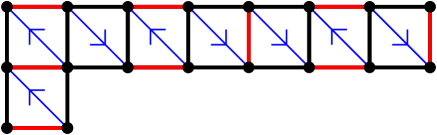
Figure 3: A perfect matching $P$ of a snake graph. The orientation $P$ induces on the diagonals is shown in blue.

3.2 Loop graphs

Roughly speaking, a loop graph is obtained from a snake graph by (potentially) creating a loop at each end. Namely, each end of the snake graph may be glued to a previous tile. Just as snake graphs enable us to obtain expansion formulae for cluster variables corresponding to plain arcs [13], loop graphs will provide us with the framework to write expansion formulae for the variables corresponding to any tagged arc.

Definition 3.6.

Let $\mathcal{G}=(G_{1},\ldots,G_{d})$ be a snake graph.
Let $c$ be an edge of $\{S(G_{1}),W(G_{1})\}$. Furthermore, let $x\in c$ denote the South-West vertex of $G_{1}$, and let $y$ denote the remaining vertex of $c$. Let $k\in\{2,\ldots,d\}$ and denote by $c^{\prime}$ the edge in $\{S(G_{k}),W(G_{k})\}$ which is a boundary edge. We let $y^{\prime}\in c^{\prime}$ denote the South-West vertex of $G_{k}$, and let $x^{\prime}$ denote the remaining vertex of $c^{\prime}$.

The loop with respect to $G_{1}$ and $k$ is obtained by gluing $c$ to $c^{\prime}$ such that $x$ (resp. $y$) is glued to $x^{\prime}$ (resp. $y^{\prime}$). By abuse of notation we also denote the resulting glued edge by $c$, and call this the cut.

We define a loop with respect to the other endtile $G_{d}$ of $\mathcal{G}$ analogously; one should just replace South and West with North and East, and choose $k\in\{1,\ldots,d-1\}$.

Definition 3.7.

A loop graph $\mathcal{G}^{\bowtie}$ is obtained from $\mathcal{G}=(G_{1},\ldots,G_{d})$ by creating a loop with respect to $G_{1}$ and $k_{1}\in\{2,\ldots,d\}$ and creating a loop with respect to $G_{d}$ and $k_{2}\in\{1,\ldots,d-1\}$.
We extend the definition to all $k_{1},k_{2}\in\{1,\ldots,d\}$ by demanding there is no loop with respect to $G_{1}$ (resp. $G_{d}$) if $k_{1}=1$ (resp. $k_{2}=d$). Consequently, loop graphs are snake graphs for which zero, one or two ends have been glued. In this paper we will always have $k_{1}\leq k_{2}$.

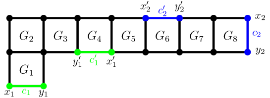
Figure 4: An example of a loop graph which has loops at both of its ends.

Definition 3.8.

As in Definition 3.7, let $\mathcal{G}^{\bowtie}$ be a loop graph obtained from a snake graph $\mathcal{G}$. A good matching of $\mathcal{G}^{\bowtie}$ is a perfect matching which can be extended to a perfect matching of $\mathcal{G}$.

Remark 3.9.

Definition 3.8 may be restated as follows. A perfect matching $P$ of $\mathcal{G}^{\bowtie}$ is a good matching if, for each cut $c$, the edges matching the vertices of $c$ both lie on the ‘same side’ of the cut. That is, when viewed as a matching of $\mathcal{G}$, $P$ must contain edge(s) matching both $x$ and $y$ or both $x^{\prime}$ and $y^{\prime}$ (but not both). We introduce the following terminology:

• $P$ is a right cut with respect to $c$ if $x$ and $y$ are matched in $\mathcal{G}$.

• $P$ is a left cut with respect to $c$ if $x^{\prime}$ and $y^{\prime}$ are matched in $\mathcal{G}$.

• $P$ is a centre cut with respect to $c$ if $P$ contains $c$.

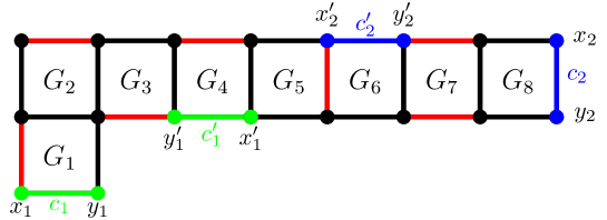
Figure 5: An example of a perfect matching $P$ (indicated by the red edges) of a loop graph which is not a good matching. Indeed, whilst $P$ is a left cut with respect to $c_{2}$, it is not a right, left nor centre cut with respect to $c_{1}$.

Proposition 3.10.

As in Proposition 3.5, any good matching $P$ of a loop graph $\mathcal{G}^{\bowtie}$ induces an orientation on the diagonal of each tile of $\mathcal{G}^{\bowtie}$.

Proof.

By definition of a good matching, $P$ can be (uniquely) extended to a perfect matching of the underlying snake graph $\mathcal{G}$. The result then follows from Proposition 3.5.

∎

4 Snake and loop graphs from surfaces

Following the work of Musiker, Schiffler and Williams we first explain how to associate snake graphs to plain arcs of $(S,M)$ with respect to ideal triangulations [13]. We then generalise this approach and associate loop graphs to all tagged arcs. The basic principle is that tiles in our snake and loop graphs correspond to quadrilaterals on the surface.

4.1 Snake graphs associated to plain arcs

4.1.1 T is an ideal triangulation without self-folded triangles

For simplicity we first restrict our attention to when $T$ is an ideal triangulation containing no self-folded triangles.

Definition 4.1.

Let $\gamma$ be a directed plain arc in $(S,M)$, and denote by $p_{1},\ldots,p_{d}$ the intersection points of $\gamma$ with $T=\{\tau_{1},\ldots,\tau_{n}\}$ (listed in order of intersection). In this way we obtain a sequence $i_{1},\ldots,i_{d}$ such that $p_{k}$ belongs to $\tau_{i_{k}}$ for each $k\in\{1,\ldots,d\}$.
Let $Q_{i_{j}}$ be a quadrilateral in $T$ with diagonal labelled by $\tau_{i_{j}}$. Let $\Delta_{j}$ and $\Delta_{j+1}$ denote the triangles in $T$ either side of $\tau_{i_{j}}$, labelled so that, with respect to the orientation of $\gamma$ through $p_{j}$, $\Delta_{j}$ precedes $\Delta_{j+1}$. We view $Q_{i_{j}}$ as a tile $G_{j}$ by deleting the diagonal $\tau_{i_{j}}$ and embedding it in the plane so that:

• the (deleted) diagonal $\tau_{i_{j}}$ of $Q_{i_{j}}$ connected the north-west and south-east vertices of $G_{j}$.

• $\Delta_{j}$ forms the lower half of $G_{j}$.

There are two possible ways to follow the rules above: if the orientation on $Q_{i_{j}}$ (induced by $(S,M)$) agrees with the orientation on $G_{j}$ (induced by the clockwise orientation of the plane) then we write $rel(G_{j})=1$; if it disagrees then $rel(G_{j})=-1$. The quantity $rel(G_{j})$ is called the relative orientation of the tile $G_{j}$ with respect to $(S,M)$.

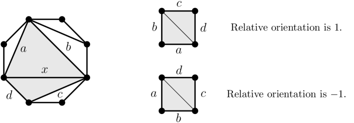
Figure 6: An example of relative orientation. The faded line indicates the deleted diagonal.

Definition 4.2.

Let $\gamma$ be a plain arc in $(S,M)$. As in Definition 4.1 we associate a tile $G_{i}$ for each intersection point, $p_{i}$, such that $rel(G_{i})\neq rel(G_{i+1})$. For each $j\in\{1,\ldots,d-1\}$ note that $\tau_{i_{j}}$ and $\tau_{i_{j+1}}$ form two sides of the triangle $\Delta_{j}$; we denote the remaining side by $\tau_{[i_{j}]}$. The snake graph $\mathcal{G}_{\gamma,T}=(G_{1},\ldots,G_{d})$ associated to $\gamma$ and $T$ is determined by gluing $G_{j}$ to $G_{j+1}$ along their common edge $\tau_{[i_{j}]}$.

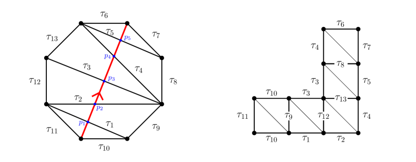
Figure 7: The construction of a snake graph from a plain arc. The thin lines indicate the associated diagonals of the tiles, however, these are not considered edges of the actual snake graph.

4.1.2 T is an arbitrary ideal triangulation

We now consider the general setup when T is an arbitrary ideal triangulation. Note that in this situation, ambiguities may arise if we followed the gluing procedures outlined in Definition 4.2. Specifically, ambiguity occurs precisely when passing through a self-folded triangle. Musiker, Schiffler and Williams [13] addressed these points using the following two definitions.

Definition 4.3.

Let $\gamma$ be an oriented plain arc. As usual, let $p_{1},\ldots,p_{d}$ denote the intersection points of $\gamma$ with $T=\{\tau_{1},\ldots,\tau_{n}\}$, and let $\tau_{i_{j}}$ denote the arc in $T$ containing $p_{j}$. We associate a tile $G_{j}$ to each $p_{j}$ as follows. If $\tau_{i_{j}}$ is not the folded side of a self-folded triangle in $T$ then $G_{j}$ is defined as in Definition 4.1, and is called an ordinary tile. Otherwise, the non-ordinary tile $G_{j}$ is defined by glueing two copies of the triangle $(\tau_{i_{j}},\tau_{i_{j-1}}=\tau_{i_{j+1}},\tau_{i_{j}})$ along $\tau_{i_{j}}$, such that the labels on the North and West (equivalently South and East) edges of $G_{j}$ are equal. As usual, in both cases, the diagonal $\tau_{i_{j}}$ is not considered an edge of $G_{j}$.

Definition 4.4.

The snake graph $\mathcal{G}_{\gamma,T}$ associated to a directed plain arc $\gamma$ is defined as follows:

• If $G_{j}$ and $G_{j+1}$ are both ordinary tiles then they are glued as in Definition 4.2.

• If $G_{j}$ is a non-ordinary tile then it is glued to $G_{j-1}$ and $G_{j+1}$ according to the arrangement illustrated in Figure 8.

For ordinary tiles we have the notion of relative orientation given in Definition 4.1. This notion is extended to each non-ordinary tile $G_{j}$ by demanding $rel(G_{j}):=-rel(G_{j-1})$. Note that the equality $rel(G_{i})=-rel(G_{i-1})$ will consequently hold for all tiles appearing in $\mathcal{G}_{\gamma,T}$.

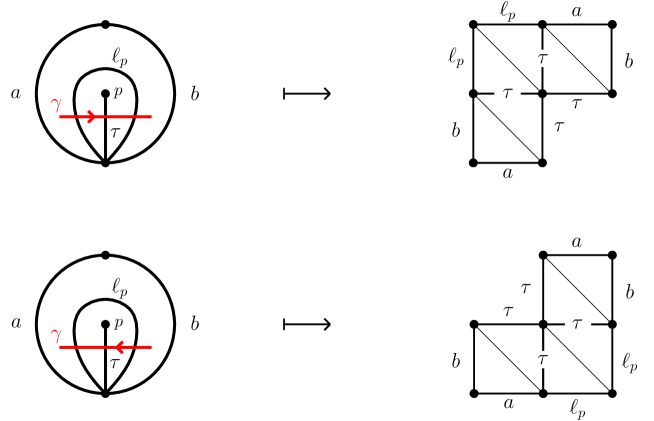
Figure 8: The gluing instructions of non-ordinary tiles in a snake graph, see Definition 4.4.

4.2 Loop graphs associated to tagged arcs

To associate loop graphs to tagged arcs it will first be helpful to introduce the notion of a hook. This was also used by Labardini-Fragoso in the context of representations of quivers with potentials [Section 6.3, [10]].

Definition 4.5.

Let $\gamma$ be a directed arc and let $T$ be an ideal triangulation. If an endpoint of $\gamma$ is incident to a puncture $p$, we define the hook at this endpoint to be the curve which:

• travels around $p$ (clockwise or anticlockwise) intersecting each incident arc at $p$ in $T$ exactly once (up to multiplicity of degree), and then follows $\gamma$, if $\gamma$ starts at the endpoint;

• or follows $\gamma$ and then travels around $p$ (clockwise or anticlockwise) intersecting each incident arc at $p$ in $T$ exactly once (up to multiplicity of degree), if $\gamma$ ends at the endpoint.

Definition 4.6.

Let $\gamma$ be a tagged arc and let $T$ be an ideal triangulation. The associated hooked arc $\overset{{}_{\backsim}}{\gamma}$ is obtained by replacing each notched endpoint of $\gamma$ with a hook.

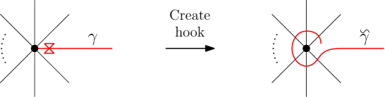
Figure 9: A hook associated to a notched endpoint. The arcs in $T$ incident to the puncture determine where the hook ends.

Definition 4.7.

Let $\gamma$ be a tagged arc such that the underlying plain arc $\gamma^{\circ}$ is not in $T$. Moreover, we suppose that $\gamma$ is not notched at any puncture enclosed by a self-folded triangle in $T$. Consider the snake graph $G_{\overset{{}_{\backsim}}{\gamma},T}=(G_{1},\ldots,G_{d})$ obtained from the associated hooked arc $\overset{{}_{\backsim}}{\gamma}$. Note that $G_{\gamma^{\circ},T}=(G_{k_{1}},\ldots,G_{k_{2}})$ is a subgraph of $G_{\overset{{}_{\backsim}}{\gamma},T}$ for some $k_{1},k_{2}\in\{1,\ldots,d\}$.
We define $G_{\gamma,T}$ to be the loop graph of $G_{\overset{{}_{\backsim}}{\gamma},T}$ with respect to loops at $G_{1},k_{1}$ and $G_{d},k_{2}$. We call $G_{\gamma,T}$ the loop graph of $\gamma$ with respect to $T$. Moreover, any loop graph $\mathcal{G}^{\bowtie}$ arising in this way is called a surface loop graph.

Remark 4.8.

Note that the hooked arc $\overset{{}_{\backsim}}{\gamma}$ is not unique, since there is a choice of orientation around the puncture at each notched endpoint. However, up to isomorphism, the resulting loop graph $G_{\gamma,T}$ is independent of this choice.

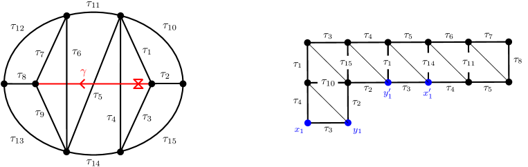
Figure 10: An example of the loop graph associated to a singly notched arc. The edge connecting $x_{1}$ and $y_{1}$ is glued to the edge connecting $x_{1}^{\prime}$ and $y_{1}^{\prime}$, where $x_{1}$ (resp. $y_{1}$) is glued to $x_{1}^{\prime}$ (resp. $y_{1}^{\prime}$).

5 Expansion formulae for tagged arcs via loop graphs

Let $T=\{\tau_{1},\ldots,\tau_{n}\}$ be an ideal triangulation with corresponding tagged triangulation $\iota(T)=\{\tau_{1}^{\prime},\ldots,\tau_{n}^{\prime}\}$. Let $x_{\tau_{1}^{\prime}},\ldots,x_{\tau_{n}^{\prime}}$ be the cluster variables corresponding to $\iota(T)$; when the context is clear we write $x_{1},\ldots,x_{n}$. In a similar fashion we associate variables to $T$: if $\tau_{i}\in T$ encloses a punctured monogon then it encloses $\tau_{i}^{\prime}$ and $\tau_{j}^{\prime}$, for some $j$, and we set $x_{\tau_{i}}:=x_{i}x_{j}$, otherwise we set $x_{\tau_{i}}:=x_{i}$. For the (principal) coefficients we set $y_{\tau_{i}}:=y_{\tau_{i}^{\prime}}:=y_{i}$ for each $i$.

Definition 5.1.

Let $T=\{\tau_{1},\ldots,\tau_{n}\}$ be an ideal triangulation and let $\gamma$ be a directed tagged arc whose underlying plain arc $\gamma^{\circ}$ is not in $T$. We denote by $\tau_{i_{1}},\ldots,\tau_{i_{d}}$ the sequence of arcs in $T$ which the associated hooked arc $\overset{{}_{\backsim}}{\gamma}$ intersects. The crossing monomial of $\gamma$ with respect to $T$ is defined as:

$$cross(\gamma,T):={\displaystyle\prod_{j=1}^{d}x_{\tau_{i_{j}}}}.$$

Definition 5.2.

Let $T=\{\tau_{1},\ldots,\tau_{n}\}$ be an ideal triangulation and let $\gamma$ be a directed arc with associated loop graph $\mathcal{G}_{\gamma,T}$. For a good matching $P$ of $\mathcal{G}_{\gamma,T}$ we define the weight monomial $x(P)$ as follows:

$$x(P):={\displaystyle\prod_{\tau_{i}\in P}x_{\tau_{i}}}.$$

Definition 5.3.

Let $T$ be an ideal triangulation and $\gamma$ a directed arc with associated loop graph $\mathcal{G}_{\gamma,T}$. Recall that every good matching $P$ of $\mathcal{G}_{\gamma,T}$ induces an orientation on the diagonals of each tile in $\mathcal{G}_{\gamma,T}$. We say the diagonal of a tile $G_{j}$ is positive with respect to some $P$ if:

• the diagonal of $G_{j}$ is oriented ‘down’ and $rel(G_{j})=1$, or

• the diagonal of $G_{j}$ is oriented ‘up’ and $rel(G_{j})=-1$,

and we say the diagonal is negative otherwise.

Example 5.4.

In Figure 3, if we suppose $rel(G_{1})=1$, then the second, third, fourth and fifth diagonals are positive diagonals, and the remaining diagonals are negative with respect to $P$.

Definition 5.5.

Let $T=\{\tau_{1},\ldots,\tau_{n}\}$ be an ideal triangulation and $\gamma$ a tagged arc. For any good matching $P$ of a loop graph $\mathcal{G}_{\gamma,T}$ we define the coefficient monomial, $y(P)$, as follows:

$$y(P):=\displaystyle\Big{(}\prod_{\begin{subarray}{c}\text{$\tau_{i_{j}}$ is a }\\ \text{positive}\\ \text{diagonal }\end{subarray}}y_{\tau_{i_{j}}}\Big{)}\Big{(}\prod_{\begin{subarray}{c}\text{$\tau_{i_{j}}$ is a radius }\\ \text{and a positive}\\ \text{diagonal}\end{subarray}}y_{\tau_{i_{j}}^{(p)}}^{-1}\Big{)}$$ (2)

where $\tau_{i_{j}}^{(p)}\in\iota(T)$ is obtained from the plain arc $\tau_{i_{j}}\in T$ by adding a notch at $p$.

Remark 5.6.

Note that, for the convenience of this paper, $y(P)$ is defined using the language of positive diagonals (first found in [15] under the name of $\gamma$-oriented diagonals), rather than the symmetric difference of $P$ with the minimal matching $P_{-}$. However, as discussed in [12], one can easily move between the two.

Theorem 5.7.

Let $(S,M)$ be a bordered surface. Let $T^{\circ}$ be an ideal triangulation with corresponding tagged triangulation $T=\iota(T^{\circ})$. Let $\mathcal{A}$ be the associated cluster algebra with principal coefficients with respect to $\Sigma_{T}=(\mathbf{x}_{T},\mathbf{y}_{T},B_{T})$. Suppose $\gamma$ is a tagged arc whose underlying plain arc $\gamma^{\circ}$ is not in $T$, and suppose that $\gamma$ is not notched at any puncture enclosed by a self-folded triangle in $T$ (for technical reasons, if $\gamma$ is doubly notched then we also assume $(S,M)$ is not twice-punctured and closed). Then the Laurent expansion of $x_{\gamma}\in\mathcal{A}$ with respect to $\Sigma_{T}$ is given by:

$$x_{\gamma}=\frac{1}{cross(\gamma,T^{\circ})}\sum_{P}x(P)y(P).$$ (3)

where the sum is taken over all good matchings $P$ of the loop graph $\mathcal{G}_{\gamma,T}$.

Remark 5.8.

In this paper, the proof of equation (3) relies on the expansion formulae of Musiker, Schiffler, Williams. Therefore, as indicated, we do not cover the case when $\gamma$ is a doubly notched arc on a twice-punctured closed surface $(S,M)$. However, the strategy employed in the upcoming work [8] can be, with enough patience, extended to cover this case too.

Example 5.9.

Consider the singly notched arc $\gamma$ and (ideal) triangulation $T$ found in Figure 10. To obtain the cluster variable $x_{\gamma}$ with respect to principal coefficients at $T$, Theorem 5.7 tells us we must compute the crossing monomial $cross(\gamma,T)$ and enumerate all good matchings of the associated loop graph (also found in Figure 10). We see

$$cross(\gamma,T)=x_{1}x_{2}x_{3}x_{4}x_{5}x_{6}$$

and the complete collection of good matchings is provided in Figure 12. We thus obtain:

$$x_{\gamma}=\frac{1}{x_{1}x_{2}x_{3}x_{4}x_{5}x_{6}}\Big{(}x_{1}x_{2}x_{4}^{2}x_{6}x_{8}+x_{1}^{2}x_{4}x_{6}x_{8}x_{15}{\color[rgb]{1,0,0}y_{3}}+x_{1}x_{2}x_{4}x_{8}x_{11}x_{14}{\color[rgb]{1,0,0}y_{5}}+x_{1}x_{3}x_{4}x_{6}x_{8}x_{10}{\color[rgb]{1,0,0}y_{2}y_{3}}$$

$$+\hskip 5.69054ptx_{1}^{2}x_{8}x_{11}x_{14}x_{15}{\color[rgb]{1,0,0}y_{3}y_{5}}+x_{1}x_{2}x_{4}x_{5}x_{7}x_{14}{\color[rgb]{1,0,0}y_{5}y_{6}}+x_{1}x_{3}x_{5}x_{7}x_{8}x_{15}{\color[rgb]{1,0,0}y_{3}y_{4}y_{5}}$$

$$+\hskip 5.69054ptx_{1}x_{3}x_{8}x_{10}x_{11}x_{14}{\color[rgb]{1,0,0}y_{3}y_{5}y_{6}}+x_{1}^{2}x_{5}x_{7}x_{14}x_{15}{\color[rgb]{1,0,0}y_{2}y_{3}y_{4}y_{5}}+x_{3}x_{5}x_{7}x_{8}x_{10}x_{11}{\color[rgb]{1,0,0}y_{3}y_{4}y_{5}y_{6}}$$

$$+\hskip 5.69054ptx_{1}x_{3}x_{5}^{2}x_{7}x_{15}{\color[rgb]{1,0,0}y_{2}y_{3}y_{5}y_{6}}+x_{1}x_{3}x_{5}x_{7}x_{10}x_{14}{\color[rgb]{1,0,0}y_{1}y_{2}y_{3}y_{4}y_{5}}+x_{2}x_{3}x_{4}x_{5}x_{8}x_{11}{\color[rgb]{1,0,0}y_{2}y_{3}y_{4}y_{5}y_{6}}$$

$$+\hskip 5.69054ptx_{3}^{2}x_{5}^{2}x_{7}x_{10}+x_{2}x_{3}x_{4}x_{5}^{2}x_{7}{\color[rgb]{1,0,0}y_{1}y_{2}y_{3}y_{4}y_{5}y_{6}}\Big{)}.$$ (4)

Example 5.10.

The reader may find it helpful to compare the loop graph expansion formulae with Musiker, Schiffler, Williams’ method. To this end, we now follow the doubly-notched example found in [Section 5.3, [13]], which we have also illustrated in Figure 11. For this choice of $\gamma$ and $T$, the collection of good matchings of $\mathcal{G}_{\gamma,T}$ is shown in Figure 13. Moreover, since

$$cross(\gamma,T)=x_{3}x_{4}x_{5}x_{6}x_{7}x_{8}$$

Theorem 5.7 gives us the following expansion of $x_{\gamma}$ with respect to principal coefficients at $T$:

$$x_{\gamma}=\frac{1}{x_{3}x_{4}x_{5}x_{6}x_{7}x_{8}}\Big{(}x_{3}x_{4}x_{6}^{2}x_{8}+x_{4}^{2}x_{6}x_{8}x_{10}{\color[rgb]{1,0,0}y_{5}}+x_{3}x_{4}x_{6}x_{8}x_{9}{\color[rgb]{1,0,0}y_{7}}+x_{2}x_{4}x_{5}x_{6}x_{8}{\color[rgb]{1,0,0}y_{3}y_{5}}$$

$$+\hskip 5.69054ptx_{4}^{2}x_{8}x_{9}x_{10}{\color[rgb]{1,0,0}y_{5}y_{7}}+x_{2}x_{4}x_{5}x_{8}x_{9}{\color[rgb]{1,0,0}y_{3}y_{5}y_{7}}+x_{4}x_{5}x_{7}x_{9}x_{10}{\color[rgb]{1,0,0}y_{5}y_{6}y_{7}}$$

$$+\hskip 5.69054ptx_{2}x_{5}^{2}x_{7}x_{9}{\color[rgb]{1,0,0}y_{3}y_{5}y_{6}y_{7}}+x_{4}x_{5}x_{6}x_{7}x_{10}{\color[rgb]{1,0,0}y_{5}y_{6}y_{7}y_{8}}+x_{3}x_{5}x_{6}x_{7}x_{9}{\color[rgb]{1,0,0}y_{3}y_{4}y_{5}y_{6}y_{7}}$$

$$+\hskip 5.69054ptx_{2}x_{5}^{2}x_{6}x_{7}{\color[rgb]{1,0,0}y_{3}y_{5}y_{6}y_{7}y_{8}}+x_{3}x_{5}x_{6}^{2}x_{7}{\color[rgb]{1,0,0}y_{3}y_{4}y_{5}y_{6}y_{7}y_{8}}\Big{)}.$$

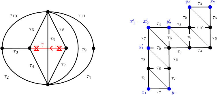
Figure 11: An example of the loop graph associated to a doubly notched arc. The edge connecting $x_{i}$ and $y_{i}$ is glued to the edge connecting $x_{i}^{\prime}$ and $y_{i}^{\prime}$, for $i\in\{1,2\}$. In this gluing $x_{i}$ (resp. $y_{i}$) is glued to $x_{i}^{\prime}$ (resp. $y_{i}^{\prime}$).

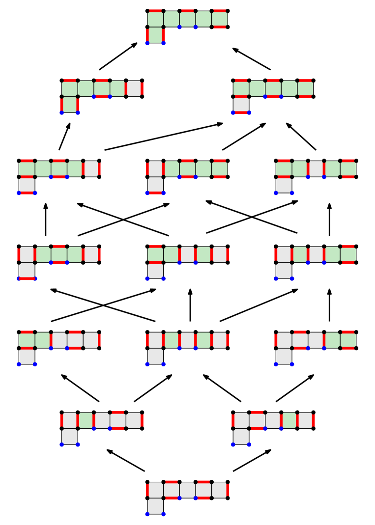
Figure 12: The lattice of good matchings of the loop graph found in Figure 10. Tiles with positive diagonals are shaded in green.

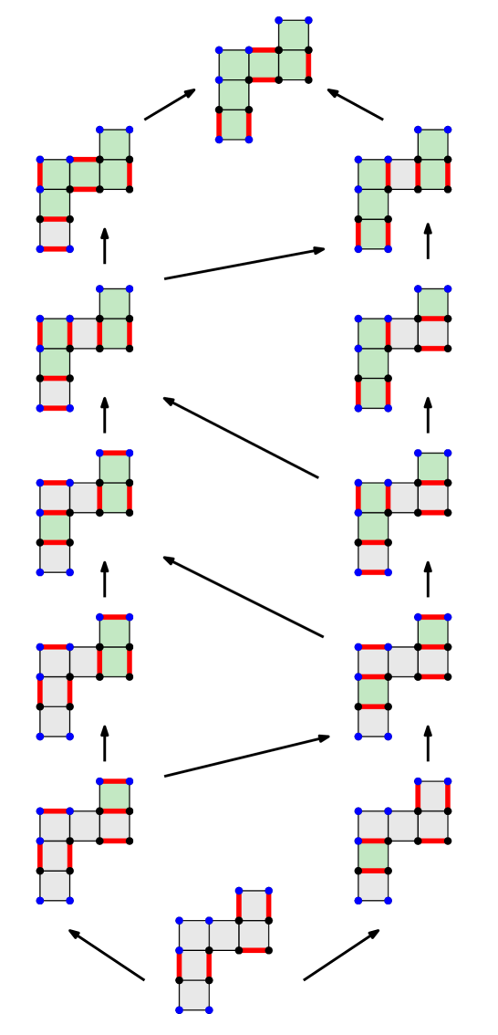
Figure 13: The lattice of good matchings of the loop graph found in Figure 11. Tiles with positive diagonals are shaded in green.

6 Proof of Theorem 5.7

We prove Theorem 5.7 by reinterpreting Musiker, Schiffler, Williams’ language of ‘$\gamma$-symmetric perfect matchings’ and ‘$\gamma$-compatible pairs of $\gamma$-symmetric perfect matchings’ as statements about good matchings of loop graphs.

6.1 $\gamma$-symmetric perfect matchings

Definition 6.1.

Let $\gamma^{(p)}$ be a tagged arc which has one end notched at a puncture $p$, and its other end tagged plain at another marked point. We call $\gamma^{(p)}$ a singly notched arc at $p$ and denote its underlying plain arc by $\gamma$. Furthermore, we denote by $\ell_{p}$ the unique plain arc enclosing $\gamma$ in a monogon with puncture $p$.

Note that if $\gamma$ has $k$ intersection points with $T^{\circ}$, then $\ell_{p}$ has $2k+l$ intersection points for $l\geq 2$. Specifically, $l$ is the degree of the puncture $p$ in $T^{\circ}$.

Definition 6.2.

Consider the snake graph $\mathcal{G}_{\ell_{p},T^{\circ}}=(G_{1},\ldots,G_{2k+l})$ and let

$$\mathcal{H}_{\gamma,1}:=(G_{1},\ldots,G_{d})\setminus\{NE(G_{k})\}$$

be the subgraph of $G_{\gamma,1}:=(G_{1},\ldots,G_{k})$ where the North-East vertex of $G_{k}$ and its incident edges $N(G_{k}),E(G_{k})$ have been removed.

Similarly, let

$$\mathcal{H}_{\gamma,2}:=(G_{k+l+1},\ldots,G_{2k+l})\setminus\{SW(G_{k+l+1})\}$$

be the subgraph of $G_{\gamma,2}:=(G_{k+l+1},\ldots,G_{2k+l})$ where the South-West vertex of $G_{k+l+1}$ and its incident edges $S(G_{k+l+1}),W(G_{k+l+1})$ have been removed.

Note that

$$\mathcal{H}_{\gamma,1}\cong\mathcal{H}_{\gamma,2}\hskip 31.29802pt\text{and}\hskip 31.29802pt\mathcal{G}_{\gamma,1}\cong\mathcal{G}_{\gamma,2}\cong\mathcal{G}_{\gamma,T^{\circ}}.$$

Definition 6.3.

A perfect matching $P$ of $\mathcal{G}_{\ell_{p},T^{\circ}}$ is said to be $\gamma$-symmetric if:

$$P_{|_{\mathcal{H}_{\gamma,1}}}\cong P_{|_{\mathcal{H}_{\gamma,2}}}$$

with respect to the isomorphism $\mathcal{H}_{\gamma,1}\cong\mathcal{H}_{\gamma,2}$.

Definition 6.4.

Let $P$ be a $\gamma$-symmetric perfect matching of $\mathcal{G}_{\ell_{p},T^{\circ}}$. The associated weight monomial and coefficient monomial are defined respectively, as follows:

$$\overline{x}(P):=\frac{x(P)}{x(P_{|_{\mathcal{G}_{\gamma,i}}})}\hskip 28.45274pt\text{and}\hskip 28.45274pt\overline{y}(P):=\frac{y(P)}{y(P_{|_{\mathcal{G}_{\gamma,i}}})}.$$

The index $i\in\{1,2\}$ above is chosen such that $P_{|_{\mathcal{G}_{\gamma,i}}}$ is a perfect matching of $\mathcal{G}_{\gamma,i}$ – this is well defined by [Lemma 12.4, [13]].

Theorem 6.5 (Theorem 4.17. [13]).

Let $(S,M)$ be a bordered surface with puncture $p$. Let $T^{\circ}$ be an ideal triangulation with corresponding tagged triangulation $T=\iota(T^{\circ})$. Let $\mathcal{A}$ be the associated cluster algebra with principal coefficients with respect to $\Sigma_{T}=(\mathbf{x}_{T},\mathbf{y}_{T},B_{T})$. Suppose $\gamma^{(p)}$ is a singly notched arc at $p$ whose underlying plain arc $\gamma$ is not in $T$, and that $p$ is not the puncture of a self-folded triangle in $T$. Then the Laurent expansion of $x_{\gamma^{(p)}}\in\mathcal{A}$ with respect to $\Sigma_{T}$ is given by:

$$x_{\gamma^{(p)}}=\frac{cross(\gamma,T^{\circ})}{cross(\ell_{p},T^{\circ})}{\displaystyle\sum_{P}\overline{x}(P)\overline{y}(P)}$$ (5)

where the sum is over all $\gamma$-symmetric perfect matchings $P$ of the snake graph $\mathcal{G}_{\ell_{p},T^{\circ}}$.

Proposition 6.6.

Let $T$ be an ideal triangulation and let $\gamma^{(p)}$ be a singly notched arc at $p$ whose underlying plain arc $\gamma$ is not in $T$, and suppose that $p$ is not the puncture of a self-folded triangle in $T$. Then there exists a bijection

$$\Phi\hskip 2.84526pt:\hskip 5.69054pt \Big{\{}\stackanchor{\text{\hskip 1.42262pt $\gamma$-symmetric perfect matchings \hskip 1.42262pt}}{\text{$P$ of $\mathcal{G}_{\ell_{p},T}$}}\Big{\}}\hskip 14.22636pt\longrightarrow\hskip 14.22636pt\Big{\{}\text{Good matchings of $\mathcal{G}_{\gamma^{(p)},T}$}$$

such that

$$\overline{x}(P)=x(\Phi(P))\hskip 14.22636ptand\hskip 14.22636pt\overline{y}(P)=y(\Phi(P))$$

for all $\gamma$-symmetric perfect matchings $P$ of $\mathcal{G}_{\ell_{p},T}$.

Proof.

Following the conventions of this section, let us write $\mathcal{G}_{\ell_{p},T}=(G_{1},\ldots,G_{2k+l})$. Note that $\mathcal{G}_{\gamma^{(p)},T}$ can be obtained from $(G_{1},\ldots,G_{k+l})$ by creating a loop with respect to $G_{k+l}$ and $k$, and can also be obtained from $(G_{k+1},\ldots,G_{2k+l})$ by creating a loop with respect to $G_{2k+l}$ and $k+1$. Furthermore, note that one of the subgraphs $(G_{k-1},G_{k},G_{k+1})$ and $(G_{k+l},G_{k+l+1},G_{k+l+2})$ is a zig-zag. Without loss of generality, we will suppose $(G_{k-1},G_{k},G_{k+1})$ is zig-zag and that $E(G_{k})$ and $S(G_{k})$ are boundary edges. Finally, note that it is possible that $\ell_{p}$ has only $l+2$ intersections with arcs in $T$, in which case $G_{k-1}=\emptyset=G_{k+l+2}$. The proof described below works in the same way for this case too.

Let $P$ be a $\gamma$-symmetric perfect matching of $\mathcal{G}_{\ell_{p},T}$. From our assumptions we see that $P$ will contain one of the (boundary) edges $E(G_{k})$ or $S(G_{k})$.

Case 1: $P$ involves $E(G_{k})$.
Note that $P$ involves the edge $E(G_{k})$ if and only if

$$P=E(G_{k})\cup P_{1}\cup P_{1}^{\prime}\cup P_{2}$$

where

• $P_{1}$ and $P_{1}^{\prime}$ are perfect matchings of $(G_{1},\ldots,G_{k-1})$ and $(G_{k+l+2},\ldots,G_{2k+l})$, respectively, such that $P_{1}\cong P_{1}^{\prime}$,

• $P_{2}$ is a perfect matching of $(G_{k+2},\ldots,G_{k+l})$.

Similarly, a good matching $P$ of $\mathcal{G}_{\gamma^{(p)},T}=(G_{1},\ldots,G_{k+l})^{\bowtie}$ is a right or centre cut at $E(G_{k})$ if and only if

$$P=P_{1}\cup P_{2}$$

where $P_{1}$ is a perfect matching of $(G_{1},\ldots,G_{k-1})$ and $P_{2}$ is a perfect matching of $(G_{k+2},\ldots,G_{k+l})$.

For the second part of the proposition, recall that $\overline{x}(P):=\frac{x(P)}{x(P_{|_{\mathcal{G}_{\gamma,1}}})}$. Since $P_{|_{\mathcal{G}_{\gamma,1}}}=E(G_{k})\cup P_{1}$ and $P_{1}\cong P_{1}^{\prime}$ then

$$\overline{x}(P)=\frac{x(E(G_{k}))x(P_{1})x(P_{1}^{\prime})x(P_{2})}{x(E(G_{k}))x(P_{1})}=x(P_{1}^{\prime})x(P_{2})=x(P_{1}\cup P_{2}).$$

Moreover, with respect to the $\gamma$-symmetric perfect matching $P$, a diagonal of a tile in $\mathcal{G}_{\gamma,1}:=(G_{1},\ldots,G_{k})$ is positive if and only if the diagonal of the corresponding tile in $\mathcal{G}_{\gamma,2}:=(G_{k+l+1},\ldots,G_{2k+l})$ is positive. Hence

$$\overline{y}(P):=\frac{y(P)}{y(P_{|_{\mathcal{G}_{\gamma,1}}})}=y(P_{1}\cup P_{2}).$$

Case 2: $P$ involves $S(G_{k})$.
Analogous to above, $P$ involves the edge $S(G_{k})$ if and only if

$$P=S(G_{k})\cup P_{1}\cup P_{1}^{\prime}\cup P_{2}\cup e_{1}\cup e_{2}$$

where

• $P_{1}$ and $P_{1}^{\prime}$ are perfect matchings of $(G_{1},\ldots,G_{k-1})\setminus E(G_{k-1})$ and $(G_{k+l+2},\ldots,G_{2k+l})\setminus b$, respectively, such that $P_{1}\cong P_{1}^{\prime}$ (here $b=W(G_{k+l+2})$ if $l$ is odd, and $b=S(G_{k+l+2})$ if $l$ is even),

• $P_{2}$ is a perfect matching of $(G_{k+1},\ldots,G_{k+l-1})$.

• $e_{1}=N(G_{k+l+1})$ and $e_{2}=S(G_{k+l+1})$ if $l$ is odd, and $e_{1}=E(G_{k+l+1})$ and $e_{2}=W(G_{k+l+1})$ if $l$ is even.

Similarly, a good matching $P$ of $\mathcal{G}_{\gamma^{(p)},T}=(G_{1},\ldots,G_{k+l})^{\bowtie}$ is a left cut at $E(G_{k})$ if and only if

$$P=S(G_{k})\cup P_{1}\cup P_{2}$$

where $P_{1}$ is a perfect matching of $(G_{1},\ldots,G_{k-1})\setminus E(G_{k-1})$ and $P_{2}$ is a perfect matching of $(G_{k+1},\ldots,G_{k+l-1})$.

For the second part of the proposition, recall that $\overline{x}(P):=\frac{x(P)}{x(P_{|_{\mathcal{G}_{\gamma,2}}})}$. Since $P_{|_{\mathcal{G}_{\gamma,2}}}=P_{1}^{\prime}\cup e_{1}\cup e_{2}$ then

$$\overline{x}(P)=\frac{x(S(G_{k}))x(P_{1})x(P_{1}^{\prime})x(P_{2})x(e_{1})x(e_{2})}{x(P_{1}^{\prime})x(e_{1})x(e_{2})}=x(S(G_{k})\cup P_{1}\cup P_{2}).$$

Moreover, as in Case 1, a diagonal of a tile in $\mathcal{G}_{\gamma,1}:=(G_{1},\ldots,G_{k})$ is positive if and only if the diagonal of the corresponding tile in $\mathcal{G}_{\gamma,2}:=(G_{k+l+1},\ldots,G_{2k+1})$ is positive. Hence

$$\overline{y}(P):=\frac{y(P)}{y(P_{|_{\mathcal{G}_{\gamma,2}}})}=y(S(G_{k})\cup P_{1}\cup P_{2}).$$

This completes the proof as any good matching of $\mathcal{G}_{\gamma^{(p)},T}=(G_{1},\ldots,G_{k+l})^{\bowtie}$ has a right, left or centre cut at $E(G_{k})$.

∎

The following observation will be helpful in the next section, where we compare good matchings and compatible pairs of $\gamma$-symmetric perfect matchings. It follows directly from the above proof.

Corollary 6.7.

Let $P$ be a $\gamma$-symmetric perfect matching of $\mathcal{G}_{\ell_{p},T}$. With respect to the set-up described in the opening paragraph of the proof of Proposition 6.6, the following holds.

If $E(G_{k})\in P$ then $P$ restricts to a perfect matching on $(G_{1},\ldots,G_{k+l})$. Moreover, we get a bijection between $\gamma$-symmetric perfect matchings of $\mathcal{G}_{\ell_{p},T}$ involving $E(G_{k})$ and good matchings of

$$\mathcal{G}_{\gamma^{(p)},T}=(G_{1},\ldots,G_{k+l})^{\bowtie}$$

with right or centre cut at $E(G_{k})$ via

$$P\mapsto P_{|_{(G_{1},\ldots,G_{k+l})}}\setminus E(G_{k}).$$

Similarly, if $S(G_{k})\in P$ then $P$ restricts to a perfect matching on $(G_{k+1},\ldots,G_{2k+l})$. Moreover, we get a bijection between $\gamma$-symmetric perfect matchings of $\mathcal{G}_{\ell_{p},T}$ involving $S(G_{k})$ and good matchings of

$$\mathcal{G}_{\gamma^{(p)},T}=(G_{1},\ldots,G_{k+l})^{\bowtie}\cong(G_{k+1},\ldots,G_{2k+l})^{\bowtie}$$

with left cut at $E(G_{k})$ via

$$P\mapsto P_{|_{(G_{k+1},\ldots,G_{2k+l})}}\setminus b$$

where $b=S(G_{k+l+1})$ if $l$ is odd and $b=W(G_{k+l+1})$ if $l$ is even.

6.2 Compatible pairs of $\gamma$-symmetric perfect matchings

Definition 6.8.

Let $\gamma^{(pq)}$ be a tagged arc which is notched at puncture $p$ and $q$ (we allow $p=q$). We say $\gamma^{(pq)}$ is a doubly notched arc at $p$ and $q$. We define $\ell_{p}$ and $\ell_{q}$ as in Definition 6.5, however, note that when $p=q$ then $\ell_{p}$ and $\ell_{q}$ are not strictly arcs as they are self-intersecting.

Definition 6.9.

Let $\gamma^{(pq)}$ be a doubly notched arc and let $P_{p}$ and $P_{q}$ be $\gamma$-symmetric perfect matchings of $\mathcal{G}_{\ell_{p},T^{\circ}}$ and $\mathcal{G}_{\ell_{q},T^{\circ}}$, respectively.
The pair $(P_{p},P_{q})$ is called $\gamma$-compatible if the following holds for some $i,j\in\{1,2\}$:

• ${P_{p}}_{|_{\mathcal{G}_{\gamma,i}}}$ and ${P_{q}}_{|_{\mathcal{G}_{\gamma,j}}}$ are perfect matchings of $\mathcal{G}_{\gamma,i}\subset\mathcal{G}_{\ell_{p},T^{\circ}}$ and $\mathcal{G}_{\gamma,j}\subset\mathcal{G}_{\ell_{q},T^{\circ}}$, respectively,

• and ${P_{p}}_{|_{\mathcal{G}_{\gamma,i}}}\cong{P_{q}}_{|_{\mathcal{G}_{\gamma,j}}}$ with respect to the canonical isomorphism $\mathcal{G}_{\gamma,i}\cong\mathcal{G}_{\gamma,j}$.

Definition 6.10.

Let $(P_{p},P_{q})$ be a $\gamma$-compatible pair of $\gamma$-symmetric perfect matchings of $(\mathcal{G}_{\ell_{p},T^{\circ}},\mathcal{G}_{\ell_{q},T^{\circ}})$. The associated cluster monomial and coefficient monomial, are defined, respectively, as follows:

$$\overline{\overline{x}}(P_{p},P_{q}):=\frac{x(P_{p})x(P_{q})}{x({P_{p}}_{|_{\mathcal{G}_{\gamma,i}}})^{3}}\hskip 28.45274pt\text{and}\hskip 28.45274pt\overline{\overline{y}}(P_{p},P_{q}):=\frac{y(P_{p})y(P_{q})}{y({P_{p}}_{|_{\mathcal{G}_{\gamma,i}}})^{3}}.$$

Where the index $i\in\{1,2\}$ is chosen such that ${P_{p}}_{|_{\mathcal{G}_{\gamma,i}}}\cong{P_{q}}_{|_{\mathcal{G}_{\gamma,j}}}$ for some $j\in\{1,2\}$, as in Definition 6.9. This is well defined by [Lemma 12.4, [13]].

Theorem 6.11 (Theorem 4.20, [13]).

Let $(S,M)$ be a bordered surface with punctures $p$ and $q$, that is not twice punctured and closed. Let $T^{\circ}$ be an ideal triangulation with corresponding tagged triangulation $T$. Let $\mathcal{A}$ be the associated cluster algebra with principal coefficients with respect to $\Sigma_{T}=(\mathbf{x}_{T},\mathbf{y}_{T},B_{T})$. Suppose $\gamma^{(pq)}$ is a doubly notched arc at $p$ and $q$ whose underlying plain arc $\gamma$ is not in $T^{\circ}$, and that neither $p$ nor $q$ are the puncture of a self-folded triangle in $T$. Then the Laurent expansion of $x_{\gamma^{(pq)}}\in\mathcal{A}$ with respect to $\Sigma_{T}$ is given by:

$$x_{(\gamma^{(pq)})}=\frac{cross(\gamma,T^{\circ})^{3}}{cross(\ell_{p},T^{\circ})cross(\ell_{q},T^{\circ})}{\displaystyle\sum_{(P_{p},P_{q})}\overline{\overline{x}}(P_{p},P_{q})\overline{\overline{y}}(P_{p},P_{q})}$$ (6)

Where the sum is over all $\gamma$-compatible pairs of $\gamma$-symmetric perfect matchings $(P_{p},P_{q})$ of the pair of snake graphs $(\mathcal{G}_{\ell_{p},T^{\circ}},\mathcal{G}_{\ell_{q},T^{\circ}})$.

Proposition 6.12.

Let $T$ be an ideal triangulation and let $\gamma^{(pq)}$ be a doubly notched arc at $p$ and $q$ whose underlying plain arc $\gamma$ is not in $T$. Furthermore, suppose that neither $p$ nor $q$ are the puncture of a self-folded triangle in $T$. Then there exists a bijection

$$\Phi\hskip 2.84526pt:\hskip 5.69054pt \Bigg{\{}\begin{subarray}{c}\text{ \normalsize$\gamma$-compatible pairs of $\gamma$-symmetric}\\ \text{ \normalsize perfect matchings $(P_{p},P_{q})$}\\ \text{ \normalsize of $(\mathcal{G}_{\ell_{p},T},\mathcal{G}_{\ell_{p},T})$}\end{subarray}\Bigg{\}}\hskip 14.22636pt\longrightarrow\hskip 14.22636pt\Big{\{}\text{Good matchings of $\mathcal{G}_{\gamma^{(pq)},T}$}\Big{\}}$$

such that

$$\overline{\overline{x}}(P_{p},P_{q})=x(\Phi(P_{p},P_{q}))\hskip 14.22636ptand\hskip 14.22636pt\overline{\overline{y}}(P_{p},P_{q})=y(\Phi(P_{p},P_{q}))$$

for all $\gamma$-compatible pairs of $\gamma$-symmetric perfect matchings $(P_{p},P_{q})$ of $(\mathcal{G}_{\ell_{p},T},\mathcal{G}_{\ell_{p},T})$.

Proof.

Let us write $\mathcal{G}_{\ell_{p},T}=(G_{1},\ldots,G_{2k+l_{p}})$ and $\mathcal{G}_{\ell_{q},T}=(H_{1},\ldots,H_{2k+l_{q}})$. Furthermore, following the same reasoning used in the proof of Proposition 6.6, without loss of generality we will suppose both $(G_{k-1},G_{k},G_{k+1})$ and $(H_{k-1},H_{k},H_{k+1})$ are zig-zag and that $E(G_{k})$,$S(G_{k})$,$E(H_{k})$,$S(H_{k})$ are boundary edges.

The collection of all $\gamma$-compatible pairs of $\gamma$-symmetric perfect matchings $(P_{p},P_{q})$ can be decomposed into the disjoint union of the following four classes:

1. $E(G_{k})\in P_{p}$ and $E(H_{k})\in P_{q}$.

2. $S(G_{k})\in P_{p}$ and $E(H_{k})\in P_{q}$.

3. $E(G_{k})\in P_{p}$ and $S(H_{k})\in P_{q}$.

4. $S(G_{k})\in P_{p}$ and $S(H_{k})\in P_{q}$.

For each class there exist $i,j\in\{1,2\}$ such that $P_{p}$ and $P_{q}$ restrict to perfect matchings on $\mathcal{G}_{\gamma,i}\subset\mathcal{G}_{\ell_{p},T}$ and $\mathcal{G}_{\gamma,j}\subset\mathcal{G}_{\ell_{q},T}$, respectively, for all $(P_{p},P_{q})$ in the chosen class. Moreover, by definition of $\gamma$-compatibility, these restrictions are isomorphic with respect to the isomorphism $\mathcal{G}_{\gamma,i}\cong\mathcal{G}_{\gamma,j}$.

This means that $P_{p}$ and $P_{q}$ can be glued along $\mathcal{G}_{\gamma,i}$ and $\mathcal{G}_{\gamma,j}$. Applying Corollary 6.7, for each of the four classes above, we get a bijection between the following classes of good matchings $P$ of $\mathcal{G}_{\gamma,T}$:

1. $P$ has a right or centre cut with respect to $E(G_{k})$ and a right or centre cut with respect to $E(H_{k})$.

2. $P$ has a left cut with respect to $E(G_{k})$ and a right or centre cut with respect to $E(H_{k})$.

3. $P$ has a right or centre cut with respect to $E(G_{k})$ and a left cut with respect to $E(H_{k})$.

4. $P$ has a left cut with respect to $E(G_{k})$ and a left cut with respect to $E(H_{k})$.

   Finally, coupling this with Proposition 6.6, the bijection $(P_{p},P_{q})\mapsto P$ described above satisfies

   $$\overline{\overline{x}}(P_{p},P_{q})=x(P)\hskip 28.45274pt\text{and}\hskip 28.45274pt\overline{\overline{y}}(P_{p},P_{q})=y(P).$$

∎

We now conclude the section with a proof of the Main Theorem 5.7.

Proof of Theorem 5.7.

When $\gamma$ is a plain arc then $\mathcal{G}_{\gamma,T}$ is just a snake graph and equation (3) reduces to [Theorem 4.10. [13]].

When $\gamma=\gamma^{(p)}$ is a singly notched arc then equation (3) follows from Theorem 6.5, Proposition 6.6 and the equality

$$cross(\gamma^{(p)},T^{\circ})=\frac{cross(\ell_{p},T^{\circ})}{cross(\gamma^{\circ},T^{\circ})}.$$

Finally, when $\gamma=\gamma^{(pq)}$ is a doubly notched arc then equation (3) follows from Theorem 6.11, Proposition 6.12 and the equality

$$cross(\gamma^{(pq)},T)=\frac{cross(\ell_{p},T^{\circ})cross(\ell_{q},T^{\circ})}{cross(\gamma^{\circ},T^{\circ})^{3}}.$$

∎

7 The lattice structure of good matchings of loop graphs

In this section we discuss some properties of surface loop graphs. It builds on the work of Musiker, Schiffler, Williams established for snake graphs in [Section 5, [14]]. We shall assume throughout that the first tile of any loop graph has relative orientation $1$.

Definition 7.1.

Let $P$ be a good matching of a loop graph $\mathcal{G}^{\bowtie}=(G_{1}\ldots,G_{d})^{\bowtie}$. We say a good matching $P^{\prime}$ of $\mathcal{G}^{\bowtie}$ is obtained from $P$ by a positive twist at tile $G_{j}$ if one of the following holds:

• $P\setminus\{N(G_{j}),S(G_{j})\}=P^{\prime}\setminus\{W(G_{j}),E(G_{j})\}$ and $j$ is odd, or

• $P\setminus\{W(G_{j}),E(G_{j})\}=P^{\prime}\setminus\{N(G_{j}),S(G_{j})\}$ and $j$ is even.

Definition 7.2.

Let $\mathcal{G}^{\bowtie}$ be a loop graph. We define the lattice of good matchings of $\mathcal{G}^{\bowtie}$ to be the quiver $L(\mathcal{G}^{\bowtie})$ whose vertices are good matchings of $\mathcal{G}^{\bowtie}$. Moreover, there is an arrow $P\rightarrow P^{\prime}$ in $L(\mathcal{G}^{\bowtie})$ if and only if $P^{\prime}$ is obtained from $P$ by a positive twist.

Definition 7.3.

Let $\mathcal{G}=(G_{1},\ldots,G_{d})$ be a snake graph. We define $Q_{\mathcal{G}}$ to be the quiver with vertices $\{1,\ldots,d\}$ and whose arrows are determined by the following rules:

• there is an arrow $i\rightarrow i+1$ in $Q_{\mathcal{G}}$ if and only if $i$ is odd and $G_{i+1}$ is on the right of $G_{i}$, or $i$ is even and $G_{i+1}$ is on top $G_{i}$,

• there is an arrow $i\rightarrow i-1$ in $Q_{\mathcal{G}}$ if and only if $i$ is odd and $G_{i}$ is on the right of $G_{i-1}$, or $i$ is even and $G_{i}$ is on top of $G_{i-1}$.

$Q_{\mathcal{G}}$ induces a poset structure on $\{1,\ldots,d\}$ by setting $i\leq j$ if and only if $i=j$ or there is a sequence of arrows in $Q_{\mathcal{G}}$ oriented from $i$ to $j$. Namely, $Q_{\mathcal{G}}$ is the Hasse diagram of this poset.

Definition 7.4.

We say $I\subseteq Q$ is an order ideal of a poset $(Q,\leq)$ if whenever $x\in I$ and $y\in Q$ satisfy $y\leq x$, then $y\in I$.

Definition 7.5.

Let $P$ be a good matching of a loop graph $\mathcal{G}^{\bowtie}=(G_{1},\ldots,G_{d})^{\bowtie}$. We define the height to be the set $h(P)\subseteq\{1,\ldots,d\}$ where $i\in h(P)$ if and only if the diagonal of $G_{i}$ is positive with respect to $P$.

Theorem 7.6 (Theorem 5.4, [14]).

Let $\mathcal{G}$ be a snake graph. Then $L(\mathcal{G})$ is isomorphic to the lattice of order ideals $\mathcal{J}(Q_{\mathcal{G}})$ of the poset $Q_{\mathcal{G}}$. Specifically, this isomorphism is given by sending a perfect matching $P$ to its height $h(P)$.

Definition 7.7.

Let $\mathcal{G}^{\bowtie}=(G_{1},\ldots,G_{d})^{\bowtie}$ be a loop graph with underlying snake graph $\mathcal{G}=(G_{1},\ldots,G_{d})$. We define the quiver $Q_{\mathcal{G}^{\bowtie}}$ of $\mathcal{G}^{\bowtie}$ to be the quiver $Q_{\mathcal{G}}$ with an additional arrow for each loop of $\mathcal{G}^{\bowtie}$. Specifically, this arrow is determined by the following rule:

• if there is a loop with respect to $G_{1}$ and $k\in\{2,\ldots,d\}$ then the arrow $1\rightarrow k$ (resp. $k\rightarrow 1$) is in $Q_{\mathcal{G}^{\bowtie}}$ if and only if $k$ is odd (resp. even) and $S(G_{k})$ is the cut edge, or $k$ is even (resp. odd) and $W(G_{k})$ is the cut edge.

• if there is a loop with respect to $G_{d}$ and $k\in\{1,\ldots,d-1\}$ then the arrow $d\rightarrow k$ (resp. $k\rightarrow d$) is in $Q_{\mathcal{G}^{\bowtie}}$ if and only if $k$ is odd (resp. even) and $N(G_{k})$ is the cut edge, or $k$ is even (resp. odd) and $E(G_{k})$ is the cut edge.

Lemma 7.8.

Let $\mathcal{G}^{\bowtie}=(G_{1},\ldots,G_{d})^{\bowtie}$ be a surface loop graph. Then $Q_{\mathcal{G}^{\bowtie}}$ defines a well-defined poset structure on $\{1,\ldots,d\}$ by setting $i\leq j$ if and only if $i=j$ or there is a sequence of arrows in $Q_{\mathcal{G}}$ oriented from $i$ to $j$.

Proof.

Suppose there is a loop with respect to $G_{1}$ and $k\in\{3,\ldots,d\}$. Since $\mathcal{G}^{\bowtie}$ is a surface loop graph then $(G_{k-2},G_{k-1},G_{k})$ and $(G_{d-1},G_{d},G_{k})$ are straight subgraphs of $\mathcal{G}^{\bowtie}$. An analogous statement holds if there a loop with respect to $G_{d}$ and $k\in\{1,\ldots,d-2\}$. Consequently, the poset structure is well defined.

∎

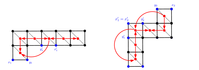
Figure 14: The associated quivers, shown in red, of the loop graphs found in Figures 10 and 11.

We are now ready to state the main theorem of this section.

Theorem 7.9.

Let $\mathcal{G}^{\bowtie}$ be a surface loop graph. Then $L(\mathcal{G}^{\bowtie})$ is isomorphic to the lattice of order ideals $\mathcal{J}(Q_{\mathcal{G}^{\bowtie}})$ of the poset $Q_{\mathcal{G}^{\bowtie}}$. Specifically, this isomorphism is given by sending a good matching $P$ to its height $h(P)$.

Proof.

Let us consider the case when $\mathcal{G}^{\bowtie}$ arises from a singly notched arc. Moreover, let $\mathcal{G}=(G_{1},\ldots,G_{k},\ldots,G_{d})$ be a snake graph which gives rise to $\mathcal{G}^{\bowtie}$ by creating a loop with respect to $G_{1}$ and $k$. Without loss of generality, we may assume that $G_{2}$ is on the right of the tile $G_{1}$, and that $(G_{k-1},G_{k},G_{k+1})$ is a zig-zag (we allow the possibility that $G_{k+1}=\emptyset$) – see Figure 15.

If $\overline{P}$ is a perfect matching of $\mathcal{G}$ that induces a negative diagonal on tile $G_{k}$ then the edge matching $x^{\prime}$ and $y^{\prime}$ is in $\overline{P}$. So $\overline{P}$ descends to a good matching on $\mathcal{G}^{\bowtie}$.
Conversely, If $\overline{P}$ is a perfect matching of $\mathcal{G}$ that induces a positive diagonal on tile $G_{k}$ then: $N(G_{k})\in\overline{P}$ or $E(G_{k})\in\overline{P}$, respective of whether $k$ is even or odd. So $\overline{P}$ descends to a good matching of $\mathcal{G}^{\bowtie}$ if and only if the edge matching $x$ and $y$ is in $\overline{P}$. Consequently, the diagonal of $G_{1}$ must also be positive.

Therefore, by Theorem 7.6, the collection of good matchings of $\mathcal{G}_{\gamma,T}$ may be identified with the order ideals of $Q_{\mathcal{G}}$ which include the vertex $1$ whenever they contain the vertex $k$. This subcollection of order ideals is precisely the order ideals of $Q_{\mathcal{G}^{\bowtie}}$, which completes the proof when $\mathcal{G}^{\bowtie}$ arises from a singly-notched arc. The doubly-notched case follows in exactly the same way.

∎

Figure 15: The setup of the loop graph $\mathcal{G}^{\bowtie}$ discussed in the proof of Theorem 7.9. The red quiver indicates (part of) the associated quiver $Q_{\mathcal{G}^{\bowtie}}$.

Corollary 7.10.

Let $\mathcal{G}^{\bowtie}$ be a surface loop graph. Then there exist (unique) good matchings $P_{-}$ and $P_{+}$ of $\mathcal{G}^{\bowtie}$ for which the diagonals of $\mathcal{G}^{\bowtie}$ are all negative and all positive, respectively. We call these the minimal and maximal good matchings of $\mathcal{G}^{\bowtie}$.

Proof.

Note that $\emptyset$ and $\{1,\ldots,d\}$ are order ideals of $Q_{\mathcal{G}^{\bowtie}}=(G_{1},\ldots,G_{d})^{\bowtie}$. By Theorem 7.9 there exist good matchings $P_{-}$ and $P_{+}$ of $\mathcal{G}^{\bowtie}$ such that $h(P_{-})=\emptyset$ and $h(P_{+})=\{1,\ldots,d\}$.

∎

Remark 7.11.

Let $\mathcal{G}^{\bowtie}$ be a loop graph. One can associate a quiver representation $M(I)$ of $Q_{\mathcal{G}^{\bowtie}}$ to each order ideal $I$ of $Q_{\mathcal{G}^{\bowtie}}$. Specifically,

$$M(i)=\mathbb{C}\hskip 11.38109pt\textit{if and only if}\hskip 11.38109pti\notin I$$

and for each arrow $\alpha:i\rightarrow j$ in $Q_{\mathcal{G}^{\bowtie}}$ we have

$$M(\alpha)=Id,\hskip 5.69054pt\text{if}\hskip 5.69054pti,j\notin I\hskip 17.07164pt\text{and}\hskip 17.07164ptM(\alpha)=0,\hskip 8.53581pt\text{otherwise}.$$

Adopting the terminology used in [3], we see from Theorem 7.9 that $L(\mathcal{G}^{\bowtie})$ is isomorphic to the canonical submodule lattice of $M(\emptyset)$, with respect to $Q_{\mathcal{G}^{\bowtie}}$, for any surface loop graph $\mathcal{G}^{\bowtie}$. Note that our situation is dual to that presented in [3], so the ordering on the canonical submodule lattice is defined by $M(I)\leq M(J)$ if and only if $M(J)$ is a submodule of $M(I)$.

E-mail address: jon.wilson@gmx.com

References

- [1] I. Canakci and R. Schiffler. Snake graph calculus and cluster algebras from surfaces. Journal of Algebra, 382:240–281, 2013.
- [2] I. Canakci and R. Schiffler. Snake graph calculus and cluster algebras from surfaces II: self-crossing snake graphs. Mathematische Zeitschrift, 281(1-2):55–102, 2015.
- [3] I. Canakci and S. Schroll. Lattice bijections for string modules, snake graphs and the weak bruhat order. arXiv preprint arXiv:1811.06064, 2018.
- [4] S. Fomin, M. Shapiro, and D. Thurston. Cluster algebras and triangulated surfaces. part I: Cluster complexes. Acta Mathematica, 201(1):83–146, 2008.
- [5] S. Fomin and D. Thurston. Cluster algebras and triangulated surfaces part II: Lambda lengths. Memoirs of the American Mathematical Society, 255(1223), 2018.
- [6] S. Fomin and A. Zelevinsky. Cluster algebras I: foundations. Journal of the American Mathematical Society, 15(2):497–529, 2002.
- [7] S. Fomin and A. Zelevinsky. Cluster algebras iv: coefficients. Compositio Mathematica, 143(1):112–164, 2007.
- [8] C. Geiss, D. Labardini-Fragoso, J. Schröer, and J. Wilson. Generic and bangle bases. In preparation.
- [9] M. Gross, P. Hacking, S. Keel, and M. Kontsevich. Canonical bases for cluster algebras. Journal of the American Mathematical Society, 31(2):497–608, 2018.
- [10] D. Labardini-Fragoso. Quivers with potentials associated with triangulations of Riemann surfaces. Ph.D. thesis, Northeastern University, 2010.
- [11] K. Lee and R. Schiffler. Positivity for cluster algebras. Annals of Mathematics, pages 73–125, 2015.
- [12] G. Musiker and R. Schiffler. Cluster expansion formulas and perfect matchings. Journal of Algebraic Combinatorics, 32(2):187–209, 2010.
- [13] G. Musiker, R. Schiffler, and L. Williams. Positivity for cluster algebras from surfaces. Advances in Mathematics, 227(6):2241–2308, 2011.
- [14] G. Musiker, R. Schiffler, and L. Williams. Bases for cluster algebras from surfaces. Compositio Mathematica, 149(2):217–263, 2013.
- [15] R. Schiffler. On cluster algebras arising from unpunctured surfaces II. Advances in Mathematics, 223(6):1885–1923, 2010.