What Happens when Separate and Unequal School Districts Merge?

Abstract

We study the welfare effects of school district consolidation, i.e. the integration of disjoint school districts into a centralised clearinghouse. We show theoretically that, in the worst-case scenario, district consolidation may unambiguously reduce students’ welfare, even if the student-optimal stable matching is consistently chosen. However, on average all students experience expected welfare gains from district consolidation, particularly those who belong to smaller and over-demanded districts. Using data from the Hungarian secondary school assignment mechanism, we compute the actual welfare gains from district consolidation in Budapest and compare these to our theoretical predictions. We empirically document substantial welfare gains from district consolidation for students, equivalent to attending a school five kilometres closer to the students’ home addresses. As an important building block of our empirical strategy, we describe a method to consistently estimate students’ preferences over schools and vice versa that does not fully assume that students report their preferences truthfully in the student-proposing deferred acceptance algorithm.

1 Introduction

For students in many countries, the transition from primary to secondary school marks an important step towards adolescence that also affects their future educational and professional careers. The modalities of this transition vary between, and sometimes also within, countries and frequently involve an element of choice whereby students can express their preferences over a set of schools. This set of alternative schools can be quite large and cover the entire country, or it can be limited to local school districts. In the latter case, every district typically constitutes an independent assignment market. School district consolidation is the process whereby previously independent assignment markets are merged so that students can now choose from a greater set of alternative schools, and can be undertaken to reduce administrative costs or to foster integration of racially and economically segregated areas. This phenomenon has taken place in the U.S. for over one hundred years: the number of school districts has fallen from 125,000 in 1900 to 84,000 in 1950 to under 15,000 today (Brasington, 1999). School district consolidations have also occurred in several other countries, e.g. in Germany (Riedel et al., 2010), Hungary (Bukodi et al., 2008), Sweden (Söderström and Uusitalo, 2010), and New Zealand (Waslander and Thrupp, 1995).

However, as in the case of the U.S., school district consolidation is rarely a smooth process and is often met with reluctance by some of the independent districts that are to integrate (Berry and West, 2008). One of the many reasons for the reluctance of districts to merge is the concern that their students will attend worse schools after consolidation takes place (Fairman and Donis-Keller, 2012). This concern is not entirely unwarranted, as district consolidation not only leads to more choice for students, but also to more competition for a place in their preferred schools. Which effect dominates is unclear a priori and depends on many factors, not least on students’ characteristics and preferences. In this paper, we shed light on the welfare effects of school district consolidation with a theoretical school choice model and with an empirical analysis of the Hungarian nationwide school assignment system.

In our theoretical model, we study district consolidation as the merger between disjoint Gale-Shapley many-to-one matching markets that are possibly different in terms of their size and their ratio between students and school seats. Students are assigned to schools using the student-optimal stable matching (SOSM) before and after consolidation takes place, but before district consolidation students can only attend schools within their own district. Although this modelling choice does not take into account several important features of the consolidation process, such as peer-effects and administrative costs, it allows us to analyse the interplay between the choice and competition effects within a school choice framework. To this end, we compare theoretically how many students attend a more (or less) preferred school after district consolidation takes place.

Example 1 shows that district consolidation can, in some cases, harm all students. In fact, for any given school choice problem, there is a way to partition the set of schools and students into districts such that we obtain this negative result (Proposition 1). The reason for this is that there is a trade-off between efficiency and stability, and the stability requirements of the SOSM become more stringent in a broader market. However, this occurs only in very particular and, some may argue, fabricated examples. To gain a more-in-depth knowledge of the welfare effects of district consolidation on the average-case scenario, we compute the expected welfare gains from consolidation for students in random markets, in which preferences are selected uniformly at random. Proposition 2 shows that district consolidation generates expected welfare gains for all students, particularly for those who belong to districts that are relatively small, or have a high ratio of local students per school seat.

These theoretical predictions are compared to empirical results that are obtained by using the data from secondary school admissions in Hungary, and in particular, from its capital city Budapest during 2015. We focus on Budapest because i) we have data on students’ stated preferences over all schools in its 23 districts, as well as schools’ priorities over all students from the 23 districts; ii) students are assigned using the student-optimal stable matching (SOSM) (Biró, 2008); iii) Hungary consolidated primary school districts in 2013 (Kertesi and Kézdi, 2013), thus the analysis of the unconsolidated case for secondary schools is particularly meaningful; and iv) we have additional data on students’ and schools’ characteristics that reveal which school features drive students’ preferences, such as schools’ previous results in mathematics and Hungarian, distance to the students’ home addresses, and socio-economic status. Our empirical strategy is to compare the SOSM in the integrated market to the matching that results in a counterfactual disintegrated market. In order to compute the counterfactual matchings, we need to construct a complete set of preferences over all market participants – schools and students. To this end, our strategy is to estimate a parametric form of students’ preferences over schools, and schools’ priorities over students. However, despite our data being remarkably detailed, we still need to overcome two technical problems here.

The first issue that needs to be addressed concerns estimating students’ preferences. In the student-proposing deferred acceptance algorithm (used to compute the SOSM) it is only a weakly dominant strategy for students to report their complete rank-order lists (ROLs) of schools truthfully. Therefore, stated ROLs may differ from the real preferences because students submit strategic ROLs by either omitting schools which they deem unattainable or by truncating their ROLs if they are confident that they will be assigned to more preferred schools. Both types of omissions have consistently been observed in the field (Chen and Pereyra, 2019) and in the lab (Castillo and Dianat, 2016); and both are particularly important for us because the average student in Budapest ranks only four schools, even when they are allowed, and encouraged, to rank all schools. The fact that students submit rather short preference lists is the reason why we need a parametric approach to construct their “true” complete ROLs. However, the fact that students may omit some of their top-ranked schools also renders standard approaches to estimate multinomial preferences inapplicable.

A second closely linked technical complication concerns the estimation of schools’ priorities: Hungarian schools only report their priorities over the set of students who actually apply to them and not over the entire set of students. In Hungary and many other countries, schools’ priorities are based on tests, interviews, and previous grades with weights decided by each school (subject to basic governmental guidelines). Therefore, the admission criteria at each school contain important idiosyncratic components that are unobservable to us. Thus, even though Fack et al. (2019) have shown how to estimate students’ preferences without assuming truth-telling behaviour, we cannot directly apply their discrete choice methods which rely on observing complete schools’ priorities over students (for example, when schools’ priorities are based on a centralised exam).

To overcome these technical challenges in preference estimation, our empirical strategy builds on two identifying assumptions. Our first assumption is that the observed assignment is stable, which implies that a student’s assigned school must be her top choice among her ex-post feasible schools (and vice versa for schools). The approach is similar to Fack et al. (2019) and Akyol and Krishna (2017). In their settings, ex-post feasible choice sets can be constructed because each student’s priority at every school is observed. This is not the case in our setting, where students’ and schools’ feasible choice sets are latent and therefore need to be endogenised to point-identify parameters. Our second identifying assumption is that students use undominated strategies, i.e. a school is ranked above another one if the former is preferred to the latter. The submitted ROLs then reveal the true partial preference order of students over schools (although they contain no information about the comparison between ranked and unranked alternatives) (Haeringer and Klijn, 2009). The method is implemented as a Gibbs sampler that imposes bounds on the latent match valuations that are derived from stability and from the observed ROLs. This approach generalises the matching estimator, proposed in Logan et al. (2008) and Menzel and Salz (2013) for the marriage market, from a one-to-one matching to a many-to-one matching setting, which is suitable for the school admissions problem studied in this paper. We test our proposed estimation method in Monte-Carlo simulations, and we find that it yields unbiased estimators for students’ preferences and schools’ priorities. Our estimator is implemented in the open source statistical software R and available online.

Our main finding is that the consolidated school market in Budapest is advantageous for the majority of students and yields significant welfare gains when compared to the counter-factual situation in which students only attend schools within their home districts. This result is robust to whether the counterfactual matching is obtained with reported or estimated students’ preferences. The welfare gains from school district consolidation are equivalent to attending a school that is five kilometres closer to the students’ home address. In other words, the average student would be willing to incur an additional travel distance of five kilometres to attend their assigned school in the consolidated market, rather than the counterfactual assigned school in their home district.

We empirically confirm our theoretical result which states that students who live in smaller districts or districts with less school capacity benefit more from school district consolidation than the average student. Also, the median student incurs a welfare gain that is positive and almost as large as the average welfare gain. To explain these large utility gains, we devise a method to decompose the total gains into a choice effect and a competition effect. We find that the substantial welfare gains are largely due to an enhanced choice set, and that the consolidated market does not lead to significantly increased competitive pressure. This can be explained by the institutional details of the school market in Hungary and in Budapest, which is characterised by a sizeable nominal overcapacity of school seats relative to the number of students. In particular, we show that the gains from school district consolidation are significantly smaller (but still positive) if we adjust the schools’ capacity to have just as many school seats as there are students in the aggregate.

The parametric specification of students’ utility from choosing a school yields insights into the determinants of students’ preferences. We find that travel distance is an important factor that determines students’ choices, but students also prefer schools with a high average academic achievement, and those with a higher average socio-economic status. Our results further imply that students dislike schools which hold additional oral entrance exams, all else equal. Moreover, we find that students have assortative preferences. For instance, students with a high socio-economic background have a stronger preference for schools with a high average socio-economic status than other students. The same holds for students who are particularly strong in Mathematics or Hungarian language.

Our results have important implications for the design of school choice markets. The consolidation of school districts generates positive, large welfare gains for students. In our empirical setting, significantly more than half of all students strictly benefit from district consolidation (between 69% to 75% of the students) and their gains are large, in particular for high-ability students. Only a small fraction of students (between 2% to 4%) are harmed by district consolidation. Our findings suggest that school admission systems should be consolidated if possible, rather than conducted independently by districts. If this was put to a vote, we find that a large majority of students would vote in favour of consolidation.

Organisation of the Paper

This paper proceeds as follows. Section 2 discusses the related literature. Section 3 presents our model and the theoretical results. Section 4 introduces our data and the Hungarian school system. Section 5 presents the estimation strategy. Section 6 showcases our empirical results, namely the welfare gains from district consolidation using both stated and estimated preferences for both students and schools. Section 7 concludes.

2 Related literature

Although there is an extensive empirical literature studying school district consolidation, the majority of it is unrelated to that of matching markets. This literature has four main findings: i) there is evidence of overall improvement in students’ performance after district consolidation, yet these improvements are not uniformly distributed and there may be losses for specific groups of students (Leach et al., 2010; Cox, 2010; Berry, 2005; Berry and West, 2008); ii) small and look-alike districts are more likely to merge (Brasington, 1999; Gordon and Knight, 2009); iii) there is empirical evidence of increased fiscal efficiency due to district consolidation (Duncombe et al., 1995; Howley et al., 2011), and iv) district consolidation has diversified the racial composition of schools (Alsbury and Shaw, 2005; Siegel-Hawley et al., 2017).

Our paper is more closely related to the literature on two-sided matching, to which we contribute on two fronts. We build on the work ofOrtega (2018, 2019), who studies the integration of different one-to-one disjoint matching markets; all of them balanced and of the same size. He shows that i) integration benefits more agents than those it harms, and ii) there are expected welfare gains from integration for all agents in random markets. We extend these results to the substantially more general setting of many-to-one matching markets in which each district has potentially different sizes and ratios between schools and students. Furthermore, we show that in any school choice problem, there exists a way to partition of students and schools into districts such that district consolidation weakly harms every student when the SOSM is consistently chosen

We assume that school districts are disjoint, whereas a related series of papers assume instead that the only the set of schools is disjoint but the pool of students is shared. This implies that some students may receive several admission offers whereas others may get none. Manjunath and Turhan (2016) and Turhan (2019) show that iterative matching procedures can lead to larger welfare gains and fewer incentives to misrepresent preferences when the initial partition of the society is coarser. Using a similar approach, Doğan and Yenmez (2017) show that students are weakly better off when all schools join a centralised clearinghouse, whereas Ekmekci and Yenmez (2019) show that no school has incentives to integrate. Hafalir et al. (2019) also study district consolidation assuming instead that districts are allowed to exchange a fraction of students as long as each student becomes better off in the exchange. They identify conditions in which stable mechanisms satisfy individual rationality, diversity, and balancedness desiderata.

All the aforementioned papers assume there is a school choice system before and after consolidation occurs, but a few others assume instead that each school conducts its own admission system before consolidation (Chade et al., 2014; Che and Koh, 2016; Hafalir et al., 2018). Some empirical papers examine students’ welfare after school choice is established (Braun et al., 2010; Machado and Szerman, 2018; Baswana et al., 2019), but to our knowledge none of those authors have studied district consolidation with school choice before and after the merge of districts occurs.

The second strand of the literature to which we contribute is the estimation of students’ preferences and schools’ priorities from observed data. The most common identifying assumption is truth-telling, where under the SOSM, a student is truth-telling if she submits her $k$ most preferred schools. Abdulkadiroğlu et al. (2017) and Che and Tercieux (2019), for example, follow this truth-telling assumption in their analysis of the New York City high school match. However, truth-telling is only a weakly dominant strategy, even when schools can be listed at no cost. Commonly observed and rationalisable strategies that are inconsistent with truth-telling include skipping “infeasible” schools and truncating ROLs after “safe” schools. Therefore, other identifying assumptions have been explored in the literature.

A less restrictive identifying assumption is that students do not swap their true preference orderings over schools when submitting a ROL, i.e. that students only use undominated strategies. Fack et al. (2019) use this assumption to estimate preferences in the Paris school choice context. This assumption is due to the fact that it is a strictly dominated strategy in the student-proposing deferred acceptance algorithm to rank school $s^{\prime}$ before school $s$ if a student actually prefers school $s$ over school $s^{\prime}$ (Haeringer and Klijn, 2009).

Another commonly used identifying assumption is stability of the observed matching, which implies that a student’s assigned school must be the top choice among her ex-post feasible schools. Stability is a more innocuous assumption than undominated strategies in that it permits inconsequential ‘mistakes’ (Artemov et al., 2017), and it can be guaranteed to prevail in large markets under fairly general conditions (Fack et al., 2019). However, empirical models that rely exclusively on the stability of the observed matching suffer from multiple stable equilibria that may exist so that the model may be ill-specified (Tamer, 2003). One way to solve this problem is by restricting the preferences in the market in order to ensure that there is a unique stable matching (Agarwal and Diamond, 2014). This approach has been applied to capital and credit markets (Sørensen, 2007; Chen, 2013) and the U.S. medical match (Agarwal, 2015). In the school choice context, this has been applied for Paris (Fack et al., 2019) and for college admissions in Mexico (Bucarey, 2018), Turkey (Akyol and Krishna, 2017), and Norway (Kirkebøen, 2012). If such assumptions are not met, then only the joint match surplus may be identifiable from observational data (Logan et al., 2008; Menzel and Salz, 2013; Menzel, 2015; Weldon, 2016). In this paper, we avoid imposing these rather restrictive assumptions on students’ preferences by developing an estimator based on the idea of Fack et al. (2019) to combine the stability assumption with the aforementioned assumption of undominated strategies. This combination allows us to point identify our parameters of interest, as we show by means of a Monte Carlo simulation.

Our methodological contribution to the literature lies in developing a method to simultaneously estimate the parametric form of students’ preferences and schools’ priorities in such settings where only partial ROLs and the final assignment are known to the econometrician, but where preferences and priorities are not perfectly aligned. We generalize the idea of Fack et al. (2019) to combine the stability and the undominated strategies assumptions to contexts where students’ feasible choice sets are unobserved, and so we extend it to include latent feasible choice sets using a data augmentation approach.

3 Model

We theoretically study district consolidation by extending the classical school choice framework of Gale and Shapley (1962) and Abdulkadiroğlu and Sönmez (2003). An extended school choice problem (ESCP) is a tuple $(T,S,\mathcal{D},\succ,\rhd,q)$, where:

• $T$ is a set of students.

• $S$ is a set of schools. We refer to $\Omega=T\cup S$ as the society.

• $q$ is the number of students that each school can accept.

• $\mathcal{D}\coloneqq\{D_{1},\ldots,D_{r}\}$ is a partition of $T\cup S$ into $r$ subsets such that each of them has some students and some schools. $T^{D_{i}}$ and $S^{D_{i}}$ denote the set of students and schools in district $D_{i}$. A population $P$ is the union of some (possibly all) districts.

• $\succ_{t}$ is the strict preference ordering of student $t$ over all schools in $S$. We write $s\succ_{t}s^{\prime}$ to denote that $t$ prefers school $s$ to school $s^{\prime}$ (and $s\succcurlyeq_{t}s^{\prime}$ if either $s\succ_{t}s^{\prime}$ or $s=s^{\prime}$). We use $\succ\coloneqq(\succ_{t})_{t\in T}$ to denote the preference profile of all students.

• $\rhd_{s}$ is the strict priority structure of school $s$ over all students in $T$. We use $t\rhd_{s}t^{\prime}$ to represent that student $t$ has a higher priority than student $t^{\prime}$ at school $s$. We use $\rhd\coloneqq(\rhd_{s})_{s\in S}$ to denote the priorities of all schools.

We assume that each district $D_{i}$ has $qn_{i}$ students, $n_{i}+k_{i}$ schools and $q(n_{i}+k_{i})$ school seats, where $k_{i}$ is a positive or negative integer that reflects the imbalance between the supply and demand for school seats in each district. If $k_{i}>0$, the district is underdemanded; if $k_{i}<0$ the district is overdemanded; if $k_{i}=0$ then the district is balanced and each student is guaranteed a seat in his own district. We will assume that $K\coloneqq\sum_{i}^{r}k_{i}\geq 0$, i.e. the society as a whole is either balanced or underdemanded and the size of its unbalance is $K$. We also use $N\coloneqq\sum_{i}^{r}n_{i}$.

The admission policy of each school $s$ is given by a choice rule $\text{Ch}_{s}:2^{T}\times\{q_{s}\}\mapsto 2^{T}$, which maps every nonempty subset $T^{\prime}\subseteq T$ of students to a subset $\text{Ch}_{s}(T^{\prime},q_{s})\subseteq T^{\prime}$ such that $\left|\text{Ch}_{s}(T^{\prime},q_{s})\right|\leq q_{s}$. We assume that for each school $s$, $\text{Ch}_{s}(\cdot,q_{s})$ is responsive to the priority ranking $\rhd_{s}$, i.e. for each $T^{\prime}\subseteq T$, $\text{Ch}_{s}(T^{\prime},q_{s})$ is obtained by choosing the highest-priority students in $T^{\prime}$ until $q_{s}$ students are chosen.

Given a population $P$ with students $T^{P}$ and schools $S^{P}$, a matching $\mu:T^{P}\cup S^{P}\mapsto T^{P}\cup S^{P}$ is a correspondence such that for each $(t,s)\in T^{P}\times S^{P}$, $\mu(t)\in S^{P}\cup\{t\}$, $\mu(s)\subseteq T^{P}$, $\left|\mu(s)\right|\leq q_{s}$ and $\mu(t)=s$ if and only if $t\in\mu(s)$. We write $\mu(t)=t$ if student $t$ is unmatched under $\mu$. A matching scheme $\sigma$ is a function that specifies a matching for each district $D_{i}$, denoted by $\sigma(\cdot,D_{i}):T^{D_{i}}\cup S^{D_{i}}\mapsto\mu:T^{D_{i}}\cup S^{D_{i}}$, as well as for the society as a whole, denoted by $\sigma(\cdot,\Omega):T\cup S\mapsto T\cup S$. As no confusion shall arise, when referring to an arbitrary district, we will simply write $\sigma(\cdot,D)$. The matchings $\sigma(\cdot,D)$ and $\sigma(\cdot,\Omega)$ denote the assignment of students to schools before and after consolidation occurs, respectively.

A matching $\mu:T^{P}\cup S^{P}\mapsto T^{P}\cup S^{P}$ is stable if $\nexists(t,s)\in T^{P}\times S^{P}$ such that i) $\mu(t)=t$ and $\left|\mu(s)\right|<q_{s}$, or ii) $s\succ_{t}\mu(t)$ and $t\rhd_{s}t^{\prime}\in\mu(s)$. The matching $\mu_{\textup{\tiny SOSM}}$ is the student-optimal stable matching if it is a stable matching and all students weakly prefer over any other stable matching. Such matching always exists and can be computed using the student-proposing deferred acceptance algorithm (Gale and Shapley, 1962; Roth and Sotomayor, 1992). A matching scheme $\sigma$ is stable if all its corresponding matchings $\sigma(\cdot,D)$ and $\sigma(\cdot,\Omega)$ are stable. We denote by $\sigma_{\textup{\tiny SOSM}}$ the matching scheme for which all its corresponding matchings (for each district and for the entire society) are student-optimal.

Welfare Effects of Consolidation

We are interested in the effect of district consolidation on students’ welfare. First, we compare the number of students who benefit after consolidation occurs against those who become worse off. The sets $T^{+}(\sigma)\coloneqq\{t\in T:\sigma(t,\Omega)\succ_{t}\sigma(t,D)\}$ and $T^{-}(\sigma)\coloneqq\{t\in T:\sigma(t,D)\succ_{t}\sigma(t,\Omega)\}$ represent the students who benefit and lose from consolidation under the matching scheme $\sigma$. In general, $T^{-}(\sigma)\neq\emptyset$, i.e. some students become worse off after consolidation. In fact, for some ESCP we have that $T^{-}(\sigma)>T^{+}(\sigma)=0$, even when $\sigma=\sigma_{\textup{\tiny SOSM}}$, i.e. even when we choose the student-optimal stable matching (SOSM) before and after consolidation, as in the following example.

Example 1.

Consider two balanced school districts $D_{1}$ and $D_{2}$, the first one with schools $s_{1},s_{2}$ and students $t_{1},t_{2}$, whereas the second one has school $s_{3}$ and student $s_{3}$. All schools have capacity one. The preferences and priorities appear below. The SOSM before consolidation occurs appears in squares, whereas the SOSM after consolidation appears in circles.

$D_{1}$	$t_{1}:\leavevmode\hbox to13.58pt{\vbox to12.2pt{\text{[drawing]}}}\succ\leavevmode\hbox to10.03pt{\vbox to10.03pt{\text{[drawing]}}}\succ s_{3}$	$\quad s_{1}:\leavevmode\hbox to10.58pt{\vbox to10.58pt{\text{[drawing]}}}\rhd t_{3}\rhd\leavevmode\hbox to12.5pt{\vbox to14.05pt{\text{[drawing]}}}$
	$t_{2}:\leavevmode\hbox to13.58pt{\vbox to12.2pt{\text{[drawing]}}}\succ\leavevmode\hbox to10.03pt{\vbox to10.03pt{\text{[drawing]}}}\succ s_{3}$	$\quad s_{2}:\leavevmode\hbox to10.58pt{\vbox to10.58pt{\text{[drawing]}}}\rhd\leavevmode\hbox to12.5pt{\vbox to14.05pt{\text{[drawing]}}}\rhd t_{3}$
$D_{2}$	$t_{3}:s_{1}\succ\leavevmode\hbox to19.46pt{\vbox to16.12pt{\text{[drawing]}}}\succ s_{2}$	$\quad s_{3}:\leavevmode\hbox to20.01pt{\vbox to16.67pt{\text{[drawing]}}}\rhd t_{1}\rhd t_{2}$

This table can be read as follows: before consolidation, student $t_{1}$ is matched to school , which is her top priority. After district consolidation, student $t_{1}$ is instead matched to school , which is only second in her rank order list. It follows that the two students from district $D_{1}$ are harmed by district consolidation, whereas the one student from district $D_{2}$ retains her initial match. Hence, the number of losers is larger than the number of winners: $\left|T^{-}(\sigma_{\textup{\tiny SOSM}})\right|=2>0=\left|T^{+}(\sigma_{\textup{\tiny SOSM}})\right|$.

Example 1 shows how consolidation can be bad for students, even when they are systematically assigned to schools using the SOSM. It can be generalised to show that, for any ESCP, we can partition the society into districts in such a way that every student is weakly better off before than after district consolidation. Formally, let $\mathcal{D^{\prime}}=\{D^{\prime}_{1},\ldots D^{\prime}_{r^{\prime}}\}$ be a partition of $T\cup S$ satisfying the following property:

$$\text{if }t\in T^{D^{\prime}_{i}}\text{ and }t\in\sigma_{\textup{\tiny SOSM}}(s,\Omega),\text{ then }s\in S^{D^{\prime}_{i}}\text{ for any }i\in\{1,\ldots,r^{\prime}\}$$ (1)

The above property says that if a student in district $D^{\prime}_{i}$ is matched after consolidation, his matched school should also be in district $D^{\prime}_{i}$. Note that because we have assumed that i) the society is either balanced or underdemanded and ii) each school is better than remaining unmatched, each student is matched after consolidation. Thus, property (1) implies that every district is either balanced or underdemanded. If this property holds, we obtain the following result.

Proposition 1 (Sometimes all students are made weakly worse-off by district consolidation).

Let $\mathcal{D^{\prime}}$ be a partition of $T\cup S$ satisfying property (1). Then $\forall t\in T$, $\sigma_{\textup{\tiny SOSM}}(t,D^{\prime})\succcurlyeq_{t}\sigma_{\textup{\tiny SOSM}}(t,\Omega)$.

Proof.

For each $x\in T\cup S$, the consolidated matching scheme $\sigma(x,D^{\prime})=\sigma_{\textup{\tiny SOSM}}(x,\Omega)$ is feasible because of condition (1), and it is also stable. This matching is, in general, different from the district-level matching scheme $\sigma_{\textup{\tiny SOSM}}(x,D^{\prime})$, as Example 1 shows, because there are fewer stability constraints imposed in the smaller school choice problem. Because $\sigma_{\textup{\tiny SOSM}}(x,D^{\prime})$ is by definition weakly preferred by each student to any other stable matching such as $\sigma$, we must have $\forall t\in T^{\Omega}$, $\sigma_{\textup{\tiny SOSM}}(t,D^{\prime})\succcurlyeq_{t}\sigma_{\textup{\tiny SOSM}}(t,\Omega)$. ∎

We can obtain such a strong negative result because of condition (1). This condition makes the extra available choices for each student worthless, as every student ends up in a school in their own district. However, the effect of added competition for school remains present, and that is why in some cases a significant fraction of all students become worse off after consolidation, as in Example 1. We emphasise that Proposition 1 is a worst-case result, and therefore tells us little about what to expect on an average instance of an ESCP. To answer this question, we examine next the average gains from district consolidation in random markets.

Random markets

Another way to analyse students’ welfare changes is to quantify the gains from district consolidation in terms of ranking of their assigned school in random ESCPs, in which the schools’ priorities and students’ preferences are generated uniformly at random.

The absolute rank of a school $s$ in the preference order of a student $t$ (over all potential schools in the society) is defined by $\textup{rk}_{t}(s)\coloneqq\left|\{s^{\prime}\in S:s^{\prime}\succcurlyeq_{t}s\}\right|$. Given a matching $\mu$, the students’ absolute average rank of schools can be defined by

$$\textup{rk}_{T}(\mu) \coloneqq \frac{1}{\left|\overline{T}\right|}\sum_{t\in\overline{T}}\textup{rk}_{t}(\mu(t))$$

where $\overline{T}$ is the set of students assigned to a school under matching $\mu$. Then, the welfare gains from consolidation for students of district $D_{i}$ are defined as

$$\gamma_{T}(\sigma_{\textup{\tiny SOSM}})=\textup{rk}_{T}(\sigma_{\textup{\tiny SOSM}}(\cdot,D_{i}))-\textup{rk}_{T}(\sigma_{\textup{\tiny SOSM}}(\cdot,\Omega))$$

Proposition 2 approximates the students’ welfare gains from consolidation as function of $n_{i}$ and $k_{i}$, providing a set of interesting comparative statistics as a corollary.

Proposition 2.

In a random ESCP, the expected welfare gains from consolidation for students $\gamma_{T}(\sigma_{\textup{\tiny SOSM}})$ can be approximated by

$$\frac{N+K}{q}\left(\frac{\log(\frac{n_{i}+k_{i}}{k_{i}})}{n_{i}}-\frac{\log(\frac{N+K}{K})}{N}\right) \text{if }k_{i}\geq 0$$ (2)

$$\frac{N+K}{q}\left(\frac{q(n_{i}+k_{i})}{n_{i}\log(\frac{n_{i}}{k_{i}})}-\frac{\log(\frac{N+K}{K})}{N}\right) \text{if }k_{i}<0$$ (3)

The above approximations have two important and testable implications for empirical studies on district consolidation, and we present them below.

Corollary 1.

The gains from consolidation are positive for all districts, in particular:

1. Students from overdemanded districts benefit more from consolidation than those from underdemanded districts (if the whole society is underdemanded).

2. A smaller size of the district size $n_{i}$ leads to larger expected welfare gains from consolidation.

Although we postpone the derivation of the approximations in Proposition 2 to appendix A, we provide some intuition for the comparative statistics below. It is well-known that, in a two-sided matching problem with different sizes, the agents in the short side choose whereas the agents in the large side get chosen, a phenomenon that increases as the imbalance between the two sides of the market grows (Ashlagi et al., 2017). Thus, if a local district is underdemanded, students get assigned to highly ranked schools before consolidation, which makes the gains from consolidation smaller. On the contrary, if students belong to an overdemanded district, they are assigned to a poorly ranked school before consolidation, which leads to large potential gains from consolidation (which indeed occur, since the whole society is underdemanded). This explains our first comparative statistic.

The second comparative statistic is due to the relationship between relative and absolute rankings. In small districts, even if students are assigned to some of their preferred schools within their district, it is unlikely that those schools are in the top of their preference list. Thus, in small districts, there is large potential for welfare gains.

4 Data

This section describes the school admission system in Hungary and the data employed. Hungary has a nation-wide integrated school market which means that every student can apply to any school in the entire country, and a centralised assignment mechanism is used to allocate students to schools. In this system, every student submits a rank order list (ROL) of arbitrary length, ranking the school programmes that he would like to attend. In turn, each school programme ranks all the students that applied to it according to several criteria such as grades, additional exams and entrance interviews. The specific weighting of these criteria is decided upon by each school but must comply with specific governmental regulations (e.g. the weight of the interview score cannot be more than 25%). School programmes submit a strict ranking of their more preferred students, whereas the remaining students are simply deemed unacceptable and are not ranked against each other. The assignment of students to schools is conducted using the deferred acceptance student-proposing algorithm (Biró, 2008). This algorithm has been used since 2000 in a fully consolidated fashion, allowing students to apply and be assigned to any school in the entire country.

For our empirical analysis, we use data from the national centralised matching of students to secondary schools in Hungary, the so-called KIFIR dataset, along with student-level data from the national assessment of basic competencies (NABC), both from the year 2015. Our data encompasses the universe of all students in Hungary who apply to a secondary school programme in 2015 (at an age of 14, with some exceptions). Each secondary school offers general or specialised study programmes with different quotas that are known ex-ante by students. The reader is referred to B.4 for details on these original data sources. Due to data protection arrangements, access to these data was restricted and our estimation routines were run by officials at the Hungarian Ministry of Education on their local computer.

We restrict our attention to the greater Budapest area which comprises 23 well-defined districts, so as to obtain a realistic setting within which the (un)consolidation of school districts can be studied. Budapest lends itself to this type of analysis because it is a geographically relatively small market that is tightly integrated, and yet the market is large enough to permit a meaningful study of the decomposition of a unified admission system into smaller and well-defined districts. Figure 1 shows the geographical area of Budapest with school district borders, and with arrows between districts that send their students to study to other districts. Figure 1 also shows that there is a considerable amount of inter-district movements, especially in the inner parts of the city.

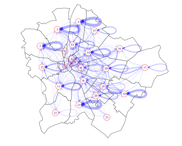
Figure 1: Flows of accepted students between school districts in Budapest. Flows from one district $D$ to another district $D^{\prime}$ are bent to the left when viewed from $D^{\prime}$. The width of the flow arrows from district $D$ to another district $D^{\prime}$ is proportional to the number of students who live in district $D$ and who were accepted at a school in district $D^{\prime}$.

We can link the application records in the KIFIR database to the corresponding information in the NABC dataset for 10,880 students who applied for a secondary school place in Budapest in 2015. In order to attain comparable competitive conditions, we adjust the schools’ capacities by removing any seats that were assigned to students not in our sample. In total, there are 881 school programmes of 246 schools that are located in the city of Budapest. A school programme sometimes contains several particular classes in which students specialize on languages or computer science, for instance. Thus, schools can offer multiple programs within the same age cohort. We aggregate school programmes at the school level in order to reduce the sample size and the associated computational burden, which is not negligible in our context. Combining the 246 schools with 10,880 students still leaves us with almost 2.7 million possible student-school combinations to be considered. We focus on three school types – four-year grammar schools, vocational secondary, and vocational schools – which the students apply to after having completed eight years of primary education. For all students in the sample, their location of residence is approximated by their zip code, and the Open Source Routing Machine (Luxen and Vetter, 2011) was used to compute travel distances from each of Hungary’s zip code centroids to every known school location.

Table 1: Secondary School Applicants in Budapest: Summary Statistics.

	Mean	SD	Min	Max	N
Panel A. Student characteristics
birth year	2,000.1	0.550	1,996	2,002	10,880
female	0.495	0.500	0	1	10,880
grade average	4.064	0.693	1.000	5.000	10,880
math score (NABC)*	0.000	1.000	$-$3.825	3.521	10,880
hungarian score (NABC)*	0.000	1.000	$-$4.186	3.176	10,880
ability†	1.472	1.398	-3.662	6.006	10,880
SES score*	0.000	1.000	$-$4.111	1.651	10,880
ROL length	4.093	1.800	1	24	10,880
applies to home district	0.680	0.466	0	1	10,880
ROL length within home district	1.054	0.965	0	7	10,880
Panel B. Attributes of first-choice school
distance (km)	7.100	4.630	0.105	36.645	10,880
ave. math score (enrolled students)	0.320	0.716	$-$1.971	1.754	10,880
ave. hungarian score (enrolled students)	0.352	0.699	$-$2.006	1.686	10,880
ave. SES score (enrolled students)	0.090	0.582	$-$1.886	1.212	10,880
Panel C. Attributes of assigned school
match rank	1.476	0.924	1.000	11.000	9,783
matched to first choice	0.711	0.453	0.000	1.000	9,783
distance (km)	7.061	4.653	0.105	36.645	9,783
assigned to home district	0.297	0.457	0.000	1.000	9,783
ave. math score (enrolled students)	0.195	0.686	$-$1.971	1.754	9,783
ave. hungarian score (enrolled students)	0.230	0.669	$-$2.006	1.686	9,783
ave. SES score (enrolled students)	$-$0.012	0.571	$-$1.886	1.212	9,783

• Variables indicated with an asterisk are z-normalized. The 2015 Hungarian and math test scores are taken by the students as part of the admissions process. ^† ability is the first principal component of the joint distribution of students’ grades, their math, and their hungarian scores. Socioeconomic status is a composite measure which includes, amongst other variables, the number of books that the household has, or the level of parental education.

Table 1 shows student-level summary statistics of our data. Panel A shows that most students were born in 2002, and that there are as many girls as boys, as one would expect. The students’ mean grade average in the previous school year is four (on a scale from one to five, where five is the highest grade in the Hungarian grading system). Their math, Hungarian, and SES scores from the NABC were standardised by us since their absolute numbers have no meaning. The variable measuring students’ socio-economic status (SES) is a composite measure that includes, amongst other variables, the number of books that the household has, or the level of parental education. This indicator was also standardized. Since the students’ grade average, their math, and their Hungarian NABC scores are highly correlated, we created a composite measure that we call “ability” and which is constructed as the first principal component of these variables. Table 1 shows that the students from Budapest in our sample file applications to about four schools, on average. Roughly seventy percent of the students apply to at least one school in their home district, and on average, students include only one school from their home district in their submitted rank order list.

Panel B shows some attributes of students’ first choice school, and panel C shows attributes of the students’ actual assigned school. Panel C shows that the average match rank is 1.46, with more than seventy percent of all students being assigned to their top choices. This is probably due to the fact that there is much excess capacity: the schools in the sample reportedly have vastly more seats than there are students (cf. tables 1 and 2). This peculiar fact has been confirmed in conversation with officials from the Hungarian ministry of education on several occasions. The distribution of the number of programmes the students apply to, and of the actual match rank in the 2015 matching round, are shown in figure 2. Figure 2 confirms that most students submit rather short ROLs, and the vast majority of students are assigned to their submitted top choice.

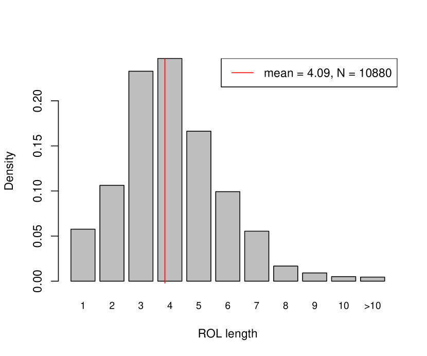
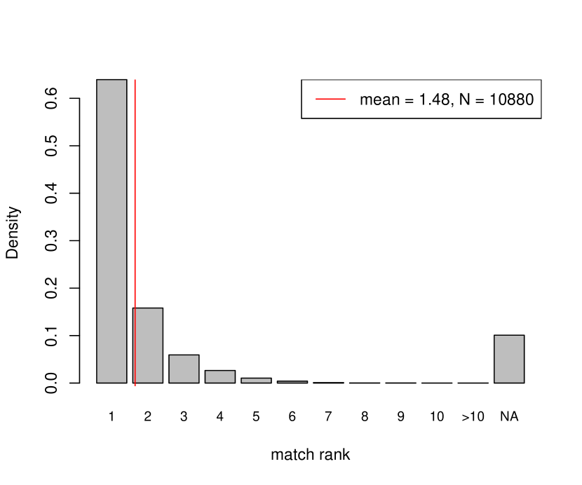
Figure 2: Distribution of the length of students’ ROLs and of their realised match rank.

Table 2 shows the school-level summary statistics. School programmes in Budapest are very attractive so that many students from outside Budapest rank a school in Budapest as their top choice. Therefore, students from Budapest face stiff competition in their “domestic” school market, and restricting the attention to students from Budapest will likely lead to a much more relaxed assignment problem. In order to circumvent this problem, we subtracted the number of admitted students from outside Budapest from the schools’ capacity so as to maintain the original “tightness” of the market – this is the adjusted capacity that is used throughout our analysis.

Table 2: Secondary Schools in Budapest: Summary Statistics.

Statistic	Mean	St. Dev.	Min	Max	N
capacity	137.098	96.306	6	502	246
adjusted capacity	116.447	90.586	6	498	246
applications	411.199	456.929	7	2,392	246
ROL1 applications	44.228	44.254	0	251	246
acceptable applications	130.638	124.433	0	698	246
assigned students	39.768	31.499	0	157	246
avg. match rank	47.229	34.011	2	187	242
entrance interview	0.439	0.497	0	1	246
enrolled students’ average
math	$-$0.130	0.778	$-$1.971	1.754	246
Hungarian	$-$0.084	0.747	$-$2.006	1.686	246
SES	$-$0.185	0.643	$-$1.886	1.212	246
assigned students’ average
math	$-$0.248	0.670	$-$2.355	1.643	246
Hungarian	$-$0.253	0.694	$-$2.332	1.476	246
SES	$-$0.135	0.638	$-$1.789	1.282	246

The average school receives over four hundred applications, of which only 130 are deemed “acceptable”. In the end, about forty students are assigned to each school on average. The comparably small number of acceptable applications could indicate that it is quite costly for schools to rank all their applicants consistently, and so they focus on only ranking those students which are most likely to be admitted to the school. Note that our estimation approach assumes that schools submit their priority lists truthfully, i.e. that every student who is labelled “unacceptable” is really less preferred than any other applicant that is actually ranked by the school. This assumption could be violated if schools strategically choose to omit very high achieving students, because they feel that these students are more likely to be admitted to a more prestigious school, and thus want to avoid the workload of prioritising these students. However, we think that this is probably a minor problem and schools are overall truth-telling.

We also collected data on whether a school holds an additional entrance interview, and we found that about forty percent of all schools do so. Table 2 also summarises the school-level averages of admitted and currently enrolled students. The standard deviation of these school-level averages is more than two-thirds of the total variance across students, which is normalised to one. Thus, there is evidence of a substantial amount of sorting by ability and socio-economic status.

5 Empirical strategy

Our empirical strategy to estimate the gains from district consolidation in a school choice market can be summarised as follows: we compute the SOSM in an unconsolidated, district-level school market and compare it to the SOSM in the consolidated, city-wide school market. In a first pass, we use the submitted rank order lists to obtain an ad hoc measure of the consolidation gains. This approach has some shortcomings since the submitted rank order lists are incomplete, as will be outlined below. To circumvent these shortcomings, we develop a procedure to estimate the complete preference order of all market participants. This allows us to compute a more complete SOSM in the unconsolidated market, and also to compare utility outcomes. Figure 3 summarises our strategy at a glance.

Figure 3: Our empirical strategy

In section 3 we have shown theoretically that one can expect overall welfare gains from school district consolidation, but that the magnitude of these gains may depend on the specific market characteristics. We test these predictions using student-level administrative data from the Hungarian school assignment system KIFIR. The KIFIR dataset contains the stated preferences of students over all schools that are included in their submitted rank order lists, and the respective rankings of schools over their applicants. These submitted rank order lists allow us to perform an ad hoc qualitative assessment of the consolidation gains in terms of foregone rank order items.

However, using the short submitted rank order lists has two shortcomings. The first problem is related to the computation of the matching in an unconsolidated district-level school market. As table 1 shows, over thirty percent of all students have not included any school from their home district in their submitted rank order lists, and on average, students included only a single school from their home district in their submitted rank order list. This is probably because the school market in Budapest has been consolidated for a long time. As a result, many students would remain unmatched in a counter-factual, disintegrated school market. Moreover, it seems reasonable to assume that students would adjust their submitted rank order lists if the school market were to be disintegrated. Thus, the SOSM in a disintegrated school market cannot be well described by using the submitted short rank order lists from the consolidated school market.

Second, it is unclear how a change in a student’s match rank translates to utility gains or losses, because the former is an ordinal concept, whereas the latter is a cardinal concept. Also, the cardinal concept of utility is more appropriate to compute aggregate welfare measures. To overcome this, we present a data augmentation approach to back out the “true” complete preference ordering from the submitted rank order lists. Our method is based on the discrete choice framework (Train, 2009) and we use it to compute the different SOSM allocations and to evaluate their welfare implications. This method is outlined in more detail in the next subsection.

5.1 Preference estimation: methodology

We observe a school choice market with a set of students ($T$) and a set of schools ($S$). We write students’ utilities over the set of schools $U_{t}(s)$, and schools’ valuations over the set of students $V_{s}(t)$ as

$$U_{t}(s) = U_{t0}+\mathbf{X}_{ts}\beta+\epsilon_{ts}$$ (4)

$$V_{s}(t) = V_{s0}+\mathbf{W}_{st}\gamma+\eta_{st}$$ (5)

where $\mathbf{X}_{ts}$ and $\mathbf{W}_{st}$ are observed characteristics that are specific to the school-student match $st$. $\mathbf{X}_{ts}$ could, for instance, include a school fixed effect or the travel distance from $t$ to $s$. The terms $U_{t0}$ and $V_{s0}$ are the outside utilities of not being matched to any student or school. These are assumed to be zero, so that the latent utilities represent the net utility of being matched. The match valuations $U_{t}(s)$ and $V_{s}(t)$ are treated as latent variables that are to be estimated along with the structural parameters $\beta$ and $\gamma$.

Throughout, we will denote by $\mathbf{U}_{t}$ the vector of student $t$’s utilities over the entire set of schools, and by $\mathbf{V}_{s}$ school $s$’s valuations over the entire set of students. We make use of the common indexing notation whereby the elements of some vector $\mathbf{Z}$ that do not refer to the student-school pair $ts$ are denoted by $\mathbf{Z}_{-ts}$, i.e. $\mathbf{U}_{-ts}$ denotes the entire set of utility numbers but for $U_{t}(s)$. We further assume that the structural error terms $\epsilon_{ts}$ and $\eta_{st}$ are independent across alternatives, and normally distributed with unit variance. While one could in principle allow for more general correlation structures, it is customary (and necessary) in the discrete choice literature to put some structure on the error terms in order to ensure identification (Train, 2009). Including a sufficiently rich set of controls and co-variates allows us to model the dependencies across alternatives in a more transparent manner than if we had left the co-variance structure completely unspecified.

We introduce some more notation for convenience below. We observe students’ submitted partial rank order lists over schools, $\mathbf{rk}$, and schools’ submitted partial priority orderings over students, $\mathbf{pr}$. Following the notation of Fack et al. (2019), we denote the observed rank order list of student $t$ as $L_{t}=(s_{t}^{1},s_{t}^{2},\ldots,s_{t}^{K_{t}})$, where $s_{t}^{k}\in\mathcal{S}$ is some school. Denote the rank that student $t$ assigns to school $s$ as $rk_{t}(s)$, with $1\leq rk_{t}(s)\leq K_{t}$ if $s\in L_{t}$ and $rk_{t}(s)=\emptyset$ else. The observed rank order lists $\mathbf{rk}$ encompass all individually observed rankings $rk_{t}(s)$. Similarly, denote the set of students who apply to school $s$ as $L_{s}$, and let the priority number that school $s$ assigns to student $t$ be $pr_{s}(t)$. Priority numbers are like ranks, in that they take discrete values, and a lower priority number means higher priority. Schools are required to prioritise all students who apply to them, but they may rank some students as “unacceptable”. We say that $pr_{s}(t)=+\infty$ if student $t$ is unacceptable to school $s$, and $pr_{s}(t)=\emptyset$ if student $t$ did not apply at school $s$. Thus, $pr_{s}(t)\in\{1,2,\ldots,|L_{s}|,\infty,\emptyset\}$.

Given the specification of the error terms and the observed rankings, equations (4) and (5) can be regarded as representing two distinct rank-ordered probit models (Train, 2009, p.181). However, the complications outlined in the introductory part of this section imply that an estimation as such is unlikely to succeed in obtaining the true preference parameters. Because schools only rank students who apply to them, and geographical distance is not an admission criterion, we cannot follow the approach of Burgess et al. (2015) to construct the feasible choice set of each student in order to identify her true preferences. For the same reason, the construction of the stability-based estimator that is proposed in Fack et al. (2019) cannot be applied. Still, we follow their idea in that we use a combination of identifying assumptions to identify the model parameters. These are described in turn.

We chose a Bayesian data augmentation approach, owing to its flexibility, and because it allows us to directly estimate the latent variables $\mathbf{U}$ and $\mathbf{V}$ which are our prime objects of interest for the purpose assessing the gains of integration. Similar approaches have been used by Logan et al. (2008) and Menzel and Salz (2013) in the context of one-to-one matching markets. Following Lancaster (2004, p.238), who describes a data augmentation approach for an ordered multinomial probit model, we simulate draws from the posterior density of the structural preference parameters $p(\beta,\gamma|data)$ by considering the component conditionals $p(\mathbf{U}|\beta,\gamma,\mathbf{V},data)$, $p(\mathbf{V}|\beta,\gamma,\mathbf{U},data)$, $p(\beta|\gamma,\mathbf{U},\mathbf{V},data)$ and $p(\gamma|\beta,\mathbf{U},\mathbf{V},data)$. We assume a vague prior for the structural preference parameters $\gamma$ and $\beta$. Details of the conditional posterior distributions are spelled out in B.2. Our data comprises the co-variates $\mathbf{X}$ and $\mathbf{W}$, of the assignment $\mu$ and of the submitted rank order and priority lists. In general, the Gibbs algorithm to sample from the posterior density can be described as follows:

1. for all $t,s$: draw $U_{t}(s)$ from $p(U_{t}(s)|\beta,\gamma,\mathbf{U}_{-ts},\mathbf{V},data)=N(\mathbf{X}_{is}\beta,1)$,
   truncated to $[\underline{U}_{t}(s),\overline{U}_{t}(s)]$

2. for all $s,t$: draw $V_{s}(t)$ from $p(V_{s}(t)|\beta,\gamma,\mathbf{V}_{-st},\mathbf{U},data)=N(\mathbf{W}_{st}\gamma,1),$
   truncated to $[\underline{V}_{s}(t),\overline{V}_{s}(t)]$

3. draw $\beta$ from $p(\beta|\gamma,\mathbf{U},\mathbf{V},data)=N\left(b,(\mathbf{X}^{\prime}\mathbf{X})^{-1}\right)$, with $b=(\mathbf{X}^{\prime}\mathbf{X})^{-1}\mathbf{X}^{\prime}\mathbf{U}$

4. draw $\gamma$ from $p(\gamma|\beta,\mathbf{U},\mathbf{V},data)=N\left(g,(\mathbf{W}^{\prime}\mathbf{W})^{-1}\right)$, with $g=(\mathbf{W}^{\prime}\mathbf{W})^{-1}\mathbf{W}^{\prime}\mathbf{V}$

5. repeat steps 1–4 $N$ times

Key to our estimation methodology are the truncation intervals for $U_{t}(s)$ and $V_{s}(t)$. These intervals are functions of the data and the latent variables in the model, and they are specific to the particular set of identifying restrictions that is used. The bounds of these intervals could be very tight, or they could encompass the entire real line. We describe possible identifying restrictions below, and outline how they can be used to construct these truncation intervals; a detailed derivation of the truncation intervals is deferred to B.1.

Weak truth-telling (WTT)

Weak truth-telling requires that the student truthfully submits his or her top-$K_{t}$ choices, and that any unranked alternative is valued less than any ranked alternative. Formally, this implies that $U_{i}(s)\geq U_{i}(s^{\prime})$ if (but not only if) $rk_{t}(s)<rk_{t}(s^{\prime})$ or $s^{\prime}\notin L_{t}$. That is, any unranked school is assumed to be less preferable than any ranked school. A similar reasoning can be applied to schools’ priorities over students, with the difference that a school $s$ cannot rank a student $t$ unless $t$ applies to $s$. However, a school can label a student as “unacceptable” which implies that all students labelled in this manner are valued less than any other ranked student. So we can bound $V_{s}(t)\geq V_{s}(t^{\prime})$ if $s\in L_{t}\cap L_{t^{\prime}}$ and $pr_{s}(t)<pr_{s}(t^{\prime})$ or $pr_{s}(t^{\prime})=+\infty$. Taken together, these bounds pin down the truncation intervals and the component conditionals in steps 1 and 2 above.

Undominated Strategies (UNDOM)

The assumption of undominated strategies is similar to that of weak truth-telling, but is restricted to the submitted rank order lists. That is, we can bound $U_{t}(s)\geq U_{t}(s^{\prime})$ if $s,s^{\prime}\in L_{t}$ and $rk_{t}(s)<rk_{t}(s^{\prime})$. The bounds for the school’s valuation over students are the same as in the weak truth-telling case because a school cannot decide not to rank a student; it must at least decide whether the student is acceptable or not. Undominated strategies is thus a weaker, but also more general, condition than weak truth-telling in the sense that the latter implies the former, but not vice versa.

Stability

If we assume that the matching of students to schools is stable in the sense outlined in section 3, a different set of bounds can be applied to the latent valuations. Denote the observed matching as $\mu$ such that $\mu(t)=s$ and $i\in\mu(s)$ if student $t$ is assigned to school $s$. Stability implies that there is no pair of a student $t$ and a school $s$ such that $V_{s}(t)>\min_{t^{\prime}\in\mu(s)}V_{s}(t^{\prime})$ (so there is no school $s$ that would like to see student $t$ enrolled rather than one of its currently enrolled students) and $U_{t}(s)>U_{t}(\mu(t))$ (no student $t$ would prefer being enrolled at $s$ rather than at his current school). This condition implies that we can bound the realization of $U_{t}(s)$ conditional on the matching $\mu$, and on the match valuations $\mathbf{U}_{-ts}$ and $\mathbf{V}_{-ts}$. Analogous bounds can be placed on $V_{s}(t)$ with straightforward extensions for cases where schools are not operating at full capacity. These bounds are spelt out in appendix B.1 in greater detail. This identifying assumption can be used on its own, or in conjunction with the assumption of undominated strategies.

5.2 Identification

Fack et al. (2019) provide an illuminating discussion of the merits of different estimation procedures in the Paris school choice context where the econometricians can observe students’ priorities at all schools. They argue that the identifying restriction stability alone allows for point-identification in large markets as in the Paris setting, but can also be used in conjunction with UNDOM. While we characterise our estimation approach in the same terms as they do, our setting differs from theirs in that the students’ relative rankings at various schools is only incompletely observed. Our preferred identifying assumption is the combination of undominated strategies and stability because it allows point identification, and it guarantees that the observed matching $\mu$ is stable under the estimated latent match valuations. The stability property is also convenient because it allows us to replicate the observed matching by computing the SOSM based on priority and preference lists that are computed from the estimated latent match valuations.

The usual conditions for identification in additive random utility models apply, and preference parameters are identified up to the variance of the unobserved random utility component which we restrict to unity. In these models, only utility differences are identified, and so we can identify only up to $J-1$ alternative-specific constants in a choice situation with $J$ alternatives, with one constant being normalised to zero. Moreover, the effect of the decision makers’ characteristics are only identified as interactions with characteristics that vary across alternatives. Furthermore, since only utility differences matter, only the differences of the error terms are identified. This is handled implicitly in our data augmentation approach, by drawing the errors subject to lower and upper bounds that are implied by the observed rank order lists. Lastly, parameters are only identified if there is sufficient heterogeneity in the observed choices: If everyone were to choose the same option, then any parameter which leads to this option being assigned a utility of plus infinity could rationalise what is observed in the data (Train, 2009; Cameron and Trivedi, 2005).

Preference parameters under the identifying restriction of weak truth-telling can in principle be identified by utilising a rank ordered model where the choice set encompasses the entire set of schools. However, because students may omit some of their most preferred schools if chances of admission are small, this assumption is often violated and parameter estimates are biased in such a model (Fack et al., 2019). To see this, consider a very popular school $s^{+}$ to which chances of admission are so small that most students, although they would rank it first, never actually include it in their submitted ROL. But then, the probability that school $s^{+}$ is the most preferred option differs from the probability that it is ranked first, and so the likelihood is misspecified. This may not be a problem at all if the researcher was merely concerned with describing the actual application behaviour of students in an existing school choice problem, but it becomes a problem if one is to study the effects of changing the rules of an existing allocation mechanism. When considering the impact of the changing of rules, it seems reasonable to assume that students’ true underlying preferences would remain unchanged, but that the changed admission rules would lead to an alteration in students’ behaviour . Therefore, an analysis that is based on student’s true preferences would retain its validity in a counter-factual allocation mechanism, while an analysis (based on reported preferences) that does not take into account strategic reporting would not be applicable.

The alternative, and weaker, identifying assumption of undominated strategies merely makes a statement about how likely it is for an individual student to prefer school $s$ over school $s^{\prime}$, given the student’s and the schools’ observable characteristics. This probability can be identified non-parametrically from the observed ROLs, conditional on $s$ and $s^{\prime}$ being part of the submitted ROL, even if some top choices, or some very unattractive alternatives, were omitted due to strategic reasoning. If we assume that the student’s decision to include both $s$ and $s^{\prime}$ in her ROL is independent of whether she ranks $s$ or $s^{\prime}$ higher, then these conditional non-parametric estimates can be matched to the unconditional model-implied probabilities, and hence the model is completely specified. Therefore, the coefficients on alternative-specific covariates can in principle be identified by their relative contribution to the probability that a particular choice $s$ is ranked before an alternative $s^{\prime}$. Of course, the usual limitations that apply in multinomial choice models also apply here; for example, preference parameters are only identified up to the scale of the error variance. In this regard we deviate from Fack et al. (2019, p.1507) who argue that an econometric model based on undominated strategies is incomplete in the sense of Tamer (2003), because “the assumption […] does not predict a unique ROL for the student”. In our Monte Carlo study, we instead find that this assumption does permit point identification of preference parameters.

If, in addition, one is willing to make the assumption that the observed matching is stable with respect to the decision makers’ true preferences, this stability assumption can serve as an additional source of identification. To illustrate this, consider some school $s^{-}$ which is so unpopular that only a few students have included it in their ROLs. Because of this, the probability that this school is preferred to some other school $s^{\prime}$ is only poorly identified, and this can lead to significant uncertainties in the parameter estimates. However, if school $s^{-}$ has some vacant seats, the stability of the observed matching implies that no other student prefers this school over their currently assigned school. In general, the stability assumption imposes additional bounds on a student’s latent match valuation if some school have vacant seats and if the student is matched to another school; or if a school’s latent valuation of this student is larger than the least valued student who is currently assigned to that school. Similar considerations apply for the bounds on schools’ valuations over students. So, the stability assumption places additional identifying restrictions on the distributions of latent errors and structural parameters.

5.3 Monte-Carlo evidence

Monte Carlo simulations provide further evidence that our method for identification works as intended. Specifically, we compare various estimation approaches that are based on different identifying assumptions as laid out above, and we show that a combination of stability and undominated strategies allows us to obtain unbiased parameter estimates with a reasonably small variance.

The data generating process of our Monte Carlo study is borrowed from Fack et al. (2019), but with slight adjustments. We consider markets with $T\in\{100,200,500\}$ students and six schools with a total capacity of $0.95\cdot T$ seats, so there is slight excess demand. Students’ utility over schools is given by

$$U_{t}(s)=\delta_{s}-d_{ts}+3\cdot(a_{t}\cdot\bar{a}_{s})+\epsilon_{ts}$$

where $\delta_{s}$ is a school fixed effect, $d_{ts}$ is the distance from student $t$ to school $s$, $a_{t}$ is the students’ grade and $\bar{a}_{s}$ is the average grade of all students at school $s$ (or put differently, the schools’ academic quality). Hence, the true preference parameter in the data generating process is a vector $\beta_{0}=(1,-1,3)^{\prime}$. $\epsilon_{ts}$ follows a standard normal distribution. For the exposition, we assume that $\delta_{s}$ is known to the econometrician and therefore enters the estimation as an additional co-variate. The schools’ valuation over students (which translates into the students’ priorities) is given by

$$V_{s}(t)=a_{t}+\eta_{st}$$

where $\eta_{is}$ is also standard normally distributed. Here, the true priority parameter $\gamma_{0}$ is a scalar equal to one. We subsume all preference and priority parameters as $\theta_{0}=(\beta_{0}^{\prime},\gamma_{0})^{\prime}$. In the market, students choose their optimal application portfolio, given their equilibrium beliefs about admission probabilities, and a small application cost. This leads some students to skip seemingly unattainable top choices, or to truncate their ROL at the bottom. As a result, the submitted ROLs are likely to violate the assumption of WTT. Based on the simulated submitted ROLs, students and school seats are matched according to the SOSM. We refer the reader to the online appendix of Fack et al. for further details.

Our major departure from their approach is with their assumption that a student’s ranking at a school is known to the econometrician. Instead, we assume that the econometrician only observes the relative rankings of students who applied at school $s$. Also, normally distributed errors are used on both sides of the market instead of the type-I extreme value distributed errors used by Fack et al..

For our Monte Carlo study, we simulated one hundred independent realisations of these markets. In the simulated markets with two hundred students, a share of 0.69 of the submitted rank order lists satisfied WTT across all simulations. For every sample $k$, we estimated students’ preferences over schools ($\hat{\beta}_{k}$), and schools’ priorities over students ($\hat{\gamma}_{k}$) using the data augmentation approach described above. In line with the recommendations laid out in Fack et al. (2019), the following different sets of identifying assumptions were used to compute the truncation intervals based on the strategically submitted ROLs:

1. weak truth-telling (WTT)

2. stability

3. undominated strategies

4. stability + undominated strategies

As a benchmark, we estimated the model under the assumption of undominated strategies based on true and complete ROLs. We let the Gibbs sampler run for 20,000 iterations, with a burn-in period of 10,000 iterations. To reduce the parameter estimates’ serial correlation, we used only every fifth sample, and discarded the rest.

Figure 4 shows box plots of the estimation errors ($\hat{\theta}_{k}-\theta_{0}$) across the one hundred realised data sets, for different estimation approaches. Table 3 shows the corresponding mean squared error and bias statistics. The first three panels of figure 4 depict the distribution of the estimation errors of students’ preference parameters ($\hat{\beta}_{k}-\beta_{0}$). As expected, the benchmark case where the complete ROLs are known on both sides allows us to identify the parameters very precisely. Furthermore, the estimates for student preferences that are derived under the assumption of weak truth-telling are biased. This too is to be expected because the assumption of weak truth-telling does not hold in the data generating process.

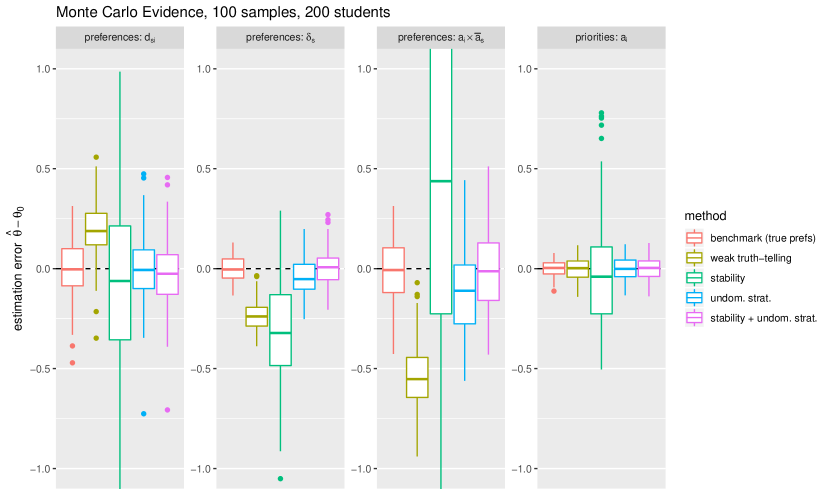
Figure 4: Box plots of the distributions of estimation errors across one hundred simulated markets (six schools with 190 seats and 200 students).

When the estimation is conducted using only the stability assumption, the results are noisy and biased. Under the stability assumption, the best estimation results are those for the coefficient on travel distances $d_{ts}$, but worse results are obtained for the schools’ quality $\delta_{s}$ and for the interaction parameter. This is in line with the previous literature on stability based estimators of preferences in small two-sided matching markets. That literature has reached a consensus that the preference parameters are only identified under certain assumptions on the observable characteristics (Weldon, 2016, pp.158-168) or certain preference structures such as perfectly aligned preferences (Agarwal and Diamond, 2014), and may not be identified at all in other circumstances. Note that this is not necessarily at odds with Fack et al. (2019) who argue that a stability based estimator can be used to point-identify preference parameters, for their stability-based estimator is based on the assumption that students’ feasible choice sets are known, whereas we assume that this is not the case.

Table 3: MSE and Bias Statistics on the Monte Carlo Simulation.

Method	Preferences			Priorities
	$d_{is}$	$\delta_{s}$	$a_{i}\cdot\bar{a}_{s}$	$a_{i}$
Panel A. Mean squared error (MSE)
benchmark (true prefs.)	0.0187	0.0038	0.0227	0.0016
weak truth–telling	0.0598	0.0581	0.3243	0.0032
stability	0.2903	0.1597	4.8612	0.0788
undominated strategies	0.0338	0.0103	0.0539	0.0030
stability + undom. strat.	0.0323	0.0088	0.0448	0.0030
Panel B. Bias
benchmark (true prefs.)	-0.0066	-0.0023	-0.0027	-0.0009
weak truth–telling	0.1937	-0.2302	-0.5425	0.0004
stability	-0.1273	-0.3132	0.9949	-0.0204
undominated strategies	0.0055	-0.0421	-0.1179	0.0001
stability + undom. strat.	-0.0219	0.0134	-0.0183	0.0026

The estimates that are derived under undominated strategies are much more precise, but also appear to suffer from a slight bias, which could be a result of the small sample size. Finally, when we combine stability and undominated strategies, our estimates are virtually indistinguishable from the benchmark estimates that are derived using the true and complete ROLs. Interestingly, estimates for the schools’ priority function are quite good in all estimation approaches, although the priority lists are only incompletely observed. This insight could lend support to alternative two-step estimators where the schools’ priority structure is estimated first, and students’ preferences are estimated in a second step, as in He and Magnac (2019).

To confirm that the combination of stability and undominated strategies is indeed able to correct the estimation bias due to strategic reporting, we compute the share of submitted ROLs satisfying WTT in each sample market, and plot this share against the parameter estimate in that sample. This is done in figure 5. Each dot in that figure represents one parameter estimate in one single simulated market. The lines represent the least square estimates for the relation between the share of ROLs that satisfy WTT and the estimation error. The corresponding regression coefficients are shown in table 4 and asterisks indicate their significance. The leftmost three panels of that figure show that the estimation error for students’ utility parameters under the WTT assumption decreases in absolute terms as the share of submitted ROLs satisfying WTT increases (green line). On the other hand, the benchmark estimates and the estimates under stability and undominated strategies are not dependent on the share of ROLs that satisfy WTT. For schools’ priority parameters, there is no significant relation between either of the estimates and the WTT share, although the point estimates are weakly positive. We conclude from this figure that the proposed estimation approach that relies on a combination of undominated strategies and stability is robust to the strategic submission of preference lists.

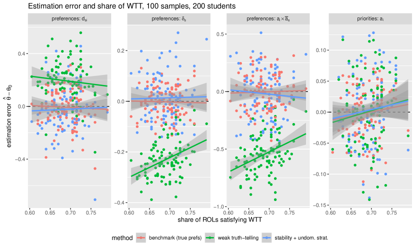
Figure 5: Dependence of the estimation error in different specifications on the share of submitted ROLs that satisfy the WTT assumption. Every dot represents one parameter estimate in one sample market. One hundred simulated markets, six schools with 190 seats, and 200 students.

Table 4: Robustness of Estimation Procedures to Violations of WTT.

Method	Preferences						Priorities
	$d_{is}$		$\delta_{s}$		$a_{i}\cdot\bar{a}_{s}$		$a_{i}$
benchmark (true prefs.)	-0.155		-0.040		0.122		0.134
weak truth–telling	-0.398		0.780	***	1.756	***	0.199
stability	0.488		0.143		-10.336	*	1.670	**
undominated strategies	0.157		0.083		-0.307		0.181
stability + undom. strat.	0.143		0.047		-0.381		0.153

• p-values indicated by ${}^{*}<0.1;{}^{**}<0.05;{}^{***}<0.01$. The table shows the coefficients from separate linear regressions of the estimation error on the share of ROLs satisfying WTT, by estimation approach and parameter. For an estimation approach to be robust to violations of the WTT assumption, the estimation error should not depend on the share of ROLs satisfying WTT.

6 Empirical results

This section reports our estimates of the gains from consolidation. First, we present results that are based on the actual submitted preference lists. Next, we present our estimates of students’ preferences that are used to construct complete preference lists. These complete preference lists are used to estimate the consolidation gains, circumventing the restrictions that are imposed by the first approach.

6.1 Gains from consolidation: using reported preferences

We first approach the problem of estimating the gains from consolidation from a purely descriptive standpoint. To this end, we take the students’ submitted rank order lists (ROLs) as given, and re-compute the SOSM under different district consolidation scenarios. As a benchmark outcome, we use the matching in the consolidated market comprising all districts in Budapest. This matching is denoted by $\mu_{BP}$ and it is almost identical to the actual matching observed in the KIFIR dataset. This matching is compared to the matching that obtains in a district-level school market ($\mu_{d}$). For every student, we compare the match rank obtained in the district-level market to the match rank in the benchmark scenario. This difference in match ranks is used as a measure for the consolidation gains.

There are two major complications with the aforementioned approach: first, a considerable number of students do not include any school from their home district in their submitted rank order list, and second, some individual school districts cannot actually accommodate all domestic students, even though there is much excess school capacity in the aggregate. These problems lead to a large number of students not being matched in the counter-factual matching. We assume that these unmatched students would prefer being matched rather than being unmatched, and that the option of being unmatched is as good as the school that they ranked last. In doing so, we obtain a lower bound for the consolidation gains.

Because district number 23 has only one single school, it does not even offer one school for every track (gymnazium, secondary or vocational). Therefore, we merge this district to its neighbouring district number 20. We show some summary statistics of the district-level and consolidated matches in table 5 below.

Table 5: Matching Statistics based on Reported Preferences.

Panel A. Unconsolidated matching
matched students	6,554
share top choice match	0.78
avg. match distance [km]	3.49
Panel B. Consolidated matching
matched students	10,494
share top choice match	0.43
share matched in home district	0.30
avg. match distance [km]	7.10

Table 6 contains a detailed account of the consolidation gains per district. That table shows that the vast majority of students is strictly better off in the consolidated market, either because they are assigned to a more preferred school in the consolidated market (29%) or because they are unmatched in the unconsolidated market (40%). Only 4% of the students are assigned to a more preferred school in the unconsolidated market. Moreover, there is not a single district in which more students would prefer the unconsolidated market over the integrated market in Budapest. Motivated by the general insights of corollary 1, figure 6 shows how the share of students who strictly gain from consolidation varies along two key dimensions: district size (left panel) and excess capacity (right panel). Figure 6(a) shows that the share of consolidation winners is practically unrelated to district size and is above fifty percent throughout. This share appears to be negatively correlated with the excess capacity in a district, as shown in Figure 6(b).

Table 6: Losers ($-$) and Winners ($+$) from Consolidation (Reported Preferences).

District	seats	students	excess seats	$-$	$0$	$+$	unmatched
1	338	95	243	3	9	26	50
2	1,191	634	557	36	241	190	148
3	928	743	185	32	263	227	213
4	865	746	119	32	319	241	151
5	625	217	408	5	50	32	122
6	1,243	172	1,071	14	24	51	77
7	1,312	212	1,100	14	73	48	70
8	2,524	290	2,234	11	79	77	119
9	2,116	275	1,841	19	73	98	77
10	2,012	591	1,421	45	120	224	194
11	1,025	713	312	13	181	169	347
12	956	359	597	17	142	108	90
13	3,290	449	2,841	44	148	152	100
14	2,893	796	2,097	52	189	247	291
15	701	454	247	11	99	120	219
16	770	659	111	1	96	162	397
17	147	628	-481	0	40	107	481
18	503	873	-370	17	177	245	432
19	773	444	329	13	68	120	237
20	1,643	573	1,070	31	157	189	189
21	2,518	641	1,877	14	258	204	157
22	273	316	-43	7	51	92	165
Total	28,646	10,880	17,766	431	2,857	3,129	4,326

• Seats refers to number of seats after removing those given to students from outside Budapest. Excess seats refers to seats minus students. The symbols $-$, $0$ and $+$ denote the number of losers, indifferences and winners from consolidation, respectively. Data obtained using stated preferences.

(a) Share of winners and district sizes

(b) Share of winners and excess capacity

Figure 6: Majority support for an integrated market in Budapest, using stated preference lists. One observation denotes one district.

To test whether these relationships are significant, we computed a linear regression of the winners’ shares per district on the size and relative excess capacity per district. Column (1) in table 7 shows that the relationship with a district’s size is insignificant, albeit estimated to be negative. The coefficient for a district’s capacity is negative and significantly different from zero.

Although the share of winners is above fifty percent in all districts, it is by no means clear that district consolidation would also be politically feasible ex ante. Our majority share measure is composed of those who strictly gain from consolidation ex post. As Fernandez and Rodrik (1991) note, ex ante uncertainty about the identity of those who gain and those who loose due to a reform induces a bias towards the status quo in majority votes. This bias can effectively prevent the implementation of a reform even when it would be supported by a majority ex post. This would be especially true for those districts where the majority share of winners is not so large.

Table 7: Testing the Relationship between Consolidation Gains and District Statistics.

	Dependent variable:
	consolidation winners’ share	average rank gain
district size (# students)	$-$0.0002	$-$0.0008
	(0.0001)	(0.0005)
relative excess capacity	$-$0.0256∗∗	$-$0.1191∗∗
	(0.0111)	(0.0478)
Observations	22	22

• ^∗p$<$0.1; ^∗∗p$<$0.05; ^∗∗∗p$<$0.01. Standard errors in parentheses, intercept not shown. One observation denotes one district. Statistics obtained using states preferences.

Next, we examine how our theoretical predictions about the distribution of quantitative rank order gains relates to our empirical results. Corollary 1 states that the expected gains from consolidation are larger for smaller markets and markets with less capacity. Figure 7(a) shows that there is practically no correlation between district size, as measured by the number of students per district, and the average rank gains from consolidation. Moreover, panel 7(b) shows that there is a strong negative partial correlation between the average rank order gains, and the districts’ excess capacity. Column (2) in table 7 contains the estimated coefficients and standard errors from a regression of average rank order gains per district on the size and capacity per district. The table shows that the coefficient for district size is rather small, and also insignificant, whereas the the coefficient for district-level capacity is significantly negative. Therefore, we find robust empirical support for the first part of Corollary 1, but we cannot statistically confirm the validity of the second part.

(a) Average rank gains and district sizes

(b) Average rank gains and excess capacityLABEL:footnote:excesscapacity

Figure 7: Rank order gains from an integrated market in Budapest, using stated preference lists. One observation denotes one district.

6.2 Preference estimation results

We now turn to the key building block of our structural approach to computing the gains from consolidation. In order to derive the complete preference ordering over schools and students, we estimate a general model of students’ preferences and schools’ priorities that was described in detail in section 5.1. See section 4 for an in depth discussion of the data sources.

We assume that students’ preferences over schools depend on the geographical distance and on the squared distance, between a student’s place of residence and the schools’ location. To proxy for the schools’ academic quality, we computed the average of the mean NABC scores in math and Hungarian of students currently enrolled at that school. Also, we computed the average SES score of those students. Finally, we included the interaction terms of the students’ math, Hungarian, and socio-economic scores with their respective school-level means in order to test whether there is evidence for assortative matching, similar to what Fack et al. (2019) find. To account for any unobserved heterogeneity across schools, we include school dummies, as we have a rather small set of observable school-level characteristics. We assume that schools select their students based on their gender, math and Hungarian NABC scores, and the SES score. The NABC scores are a proxy for the outcome of a nationwide assessment which we do not observe. We estimated a separate set of coefficients for each tier of the Hungarian school system. Our Gibbs sampler was initialized with zero values for all parameters and valuations. Because the estimation procedure is rather time consuming, we let it run for only ten thousand iterations and discarded the first five thousand iterations. To reduce the serial correlation, only every tenths estimate of the remaining five thousand iterations was used so that the posterior means are averaged across five hundred iterations. By visual inspection, we confirmed that the coefficient estimates had converged to their stationary posterior distribution after about two thousand iterations.

The posterior means of the parameter estimates for two different identifying assumptions that were discussed in section 5.1 – weak truth-telling (WTT), and stability in combination with undominated strategies – are shown in table 8 below and will be discussed in turn. Notice that our Bayesian estimation approach allows us to directly sample from the posterior parameter distribution, so that we do not need to rely on asymptotic results as in conventional estimation approaches. That is why table 8 does not include asymptotic p-values but instead shows the 95% confidence intervals of the posterior distribution.

Table 8: Posterior Parameter Means under Two Different Identifying Assumptions.

Student’s selection of schools	stability + undom.		WTT
	$\bar{\beta}$	95% CI	$\bar{\beta}$	95% CI
distance (km)	-0.148	[-0.152;-0.144]	-0.339	[-0.341;-0.336]
distance (km2)	0.002	[ 0.002; 0.003]	0.007	[ 0.007; 0.007]
academic quality	0.750	[ 0.681; 0.818]	1.487	[ 1.458; 1.515]
avg. SES	1.520	[ 1.411; 1.650]	0.462	[ 0.418; 0.509]
oral entrance exam	-1.457	[-1.698;-1.240]	-4.436	[-4.587;-4.288]
math $\times$ ave. math	0.183	[ 0.166; 0.196]	0.185	[ 0.175; 0.195]
hungarian $\times$ ave. Hungarian	0.222	[ 0.205; 0.237]	0.303	[ 0.293; 0.315]
SES $\times$ ave. SES	0.294	[ 0.279; 0.308]	0.356	[ 0.347; 0.368]
Schools’ selection of students	$\bar{\gamma}$	95% CI	$\bar{\gamma}$	95% CI
gymnazium
female	-0.930	[-0.947;-0.909]	-0.013	[-0.040; 0.014]
math score	0.049	[ 0.033; 0.066]	0.194	[ 0.171; 0.218]
Hungarian score	0.394	[ 0.376; 0.413]	0.224	[ 0.199; 0.249]
SES score	0.038	[ 0.024; 0.053]	0.096	[ 0.076; 0.116]
secondary school
female	-0.439	[-0.481;-0.401]	0.124	[ 0.089; 0.159]
math score	0.184	[ 0.163; 0.205]	0.236	[ 0.208; 0.265]
Hungarian score	0.287	[ 0.262; 0.315]	0.231	[ 0.203; 0.259]
SES score	0.053	[ 0.032; 0.072]	0.103	[ 0.082; 0.123]
vocational school
female	0.094	[ 0.043; 0.158]	0.051	[-0.031; 0.131]
math score	0.101	[ 0.063; 0.136]	0.078	[ 0.025; 0.129]
Hungarian score	0.189	[ 0.152; 0.226]	0.144	[ 0.089; 0.200]
SES score	0.011	[-0.023; 0.044]	0.015	[-0.020; 0.051]

• Posterior means of preference and priority parameters under two different identifying assumptions. Fixed effects for schools numbered 2 through to 243 were included in students’ preference equation and are not reported here. Confidence intervals from the posterior parameter distribution of the Gibbs sampler.

First, consider the results of the college selection equation (top panel of table 8) across the two identifying assumptions. These results are qualitatively similar to each other: students dislike schools that are further away from them, but the marginal disutility of travelling is decreasing because the squared distance term is positive. Students also value academic quality and prefer schools with a higher average SES score, but they dislike the presence of an oral entrance exam. The coefficient for the presence of an entrance exam is much smaller (i.e. more negative) in the WTT result: this is an indication that students strategically omit highly competitive schools which hold an entrance exam, so that the WTT estimates of the oral interview are biased downwards, whereas our stability based estimator corrects for this bias. This result confirms how important it is correct for biases due to strategic reporting when estimating students’ preferences. The interaction terms are all positive, which suggests that there is sorting on both academic ability and on socioeconomic background. Both estimation approaches yield results that are qualitatively quite similar. Note that the variance of the interacted variables is much larger than that of the school-level variables, so that the interaction terms’ contribution towards explaining student preferences is actually quite large.

The results of the student selection equation (bottom panel) show that students’ math and Hungarian scores are important variables that schools condition their choices on. Somewhat surprisingly, the female coefficient is negative in the stability + undom. specification, whereas it is minimal in the WTT specification. The large negative estimated coefficients for the female indicator is due to the stability requirement: in the data, female students have higher Hungarian scores than male students. At the same time, the Hungarian score is also a key determinant of the schools’ priority decision. But in the aggregate, roughly as many female students as male students are admitted to each school, and so the negative female coefficient is needed to ensure that not too many female students form instabilities with school seats occupied by male students. Hence, we think that the negative female coefficient merely reflects the schools’ desire to have a balanced gender composition, but it does not indicate discrimination of female students per se.

All schools except for vocational schools appear to select on the students’ socioeconomic status although the coefficient is rather small compared to the Hungarian score. Yet, in combination with the students’ taste for schools with a higher average socio-economic status, and the tendency of students with higher socio-economic backgrounds to prefer schools with a higher average socio-economic status, these results may be indicative of social sorting patterns that could be interesting in their own right.

Constructing complete preference lists

In order to obtain complete preference lists for the entire market, we use the estimated coefficients of the student and school selection equations as represented in table 8 and combine them with one set of draws from the distribution of error terms that respect the upper and lower bounds derived from stability and imposed by submitted preference lists. Thus, the estimated utility for student $i$ visiting school $s$ is

$$\hat{U}_{t}(s)=\mathbf{X}_{ts}\bar{\beta}+\hat{\epsilon}_{ts}$$

where $\hat{\epsilon}_{ts}$ is one particular realization of the latent error distribution such that $\hat{U}_{t}(s)$ respects the bounds that are imposed by the identifying assumptions. This estimated latent utility comes straight from the Gibbs sampler. Schools’ latent match utilities are constructed analogously. These estimates of the latent valuations can then be used to construct, for each market participant, a complete preference ordering of the other market side. Note however, that every such set of valuations is only one particular draw from an infinite manifold of possible realizations. Currently, we only use a single realization of the valuations, and we believe that the large market size validates this approach.

6.3 Gains from consolidation: using estimated preferences

We now repeat the analysis of section 6.1 above, but using the complete rank order lists described above. Again, we compare the outcome of a consolidated city-wide match to the district-level matching scheme. Instead of the rank order gains, we computed the average gains in latent utility. For a student $t$, this is defined as the utility difference between visiting the assigned school in the consolidated market, $\mu_{BP}(t)$, and the assigned school in the district level market, $\mu_{d}(t)$:

$$\Delta U_{t}\equiv\hat{U}_{t}(\mu_{BP}(t))-\hat{U}_{t}(\mu_{d}(t))$$

Utility is a unitless quantity which is hard to interpret per se, but our utility specification allows us to express these gains in terms of travel distances:

$$\Delta U_{t}^{km}\approx\frac{\Delta U_{t}}{\left|\frac{\partial\hat{U}_{t}(\mu_{BP}(t))}{\partial d_{t\mu_{BP}(t)}}\right|},$$

with $d_{t\mu_{BP}(t)}$ being the travel distance between student $t$’s zip code of residence and her assigned school in the consolidated market. Because students dislike utility, we use the absolute value in the denominator, so that $\Delta U_{t}^{km}>0$ corresponds to a positive welfare gain due to market consolidation. Therefore, $\Delta U_{t}^{km}$ is a measure of the additional travel time that a student would be willing to incur in order to visit the school in the consolidated market, rather than the assigned school in the district level school market. As before, we merge district 23 to its neighbouring district number 20. We also conducted the same analysis with artificially balanced markets where the number of school seats was equal to the number of students in every district. Those results are reported in B.6.

Table 9 shows some summary statistics of the resulting district-level and consolidated, city-wide matchings. Table 9 shows that some students remain unmatched in the district-level matching. This is because the school market in Budapest has been an integrated one for a long time already, so some districts do not have enough school seats to accommodate all students of their own district. In the consolidated market, all students are matched because there is enough capacity in the aggregate, and because preference lists are complete.

Table 9: Matching Statistics based on Estimated Preferences.

Panel A. Unconsolidated matching
matched students	9,986
share top choice match	0.83
avg. match distance [km]	3.55
Panel B. Consolidated matching
matched students	10,880
share top choice match	0.66
share matched in home district	0.29
avg. match distance [km]	7.14

Table 10 shows that the vast majority of students (67%) strictly benefit from participating in a consolidated market. Only 2% of the students are assigned to a less preferred school under the consolidated assignment. As in the analysis made with stated preferences, we observe that more students benefit from district consolidation than those that are harmed, and this observation holds for every single school district.8% of the students remain unassigned in the unconsolidated market because there are three school districts with more students than school seats.

Table 10: Losers ($-$) and Winners ($+$) from Consolidation (Estimated Preferences).

District	seats	students	excess seats	$-$	$0$	$+$	unmatched
1	338	95	243	3	9	83	0
2	1,191	634	557	3	216	415	0
3	928	743	185	3	253	487	0
4	865	746	119	8	273	465	0
5	625	217	408	2	43	172	0
6	1,243	172	1,071	8	20	144	0
7	1,312	212	1,100	3	81	128	0
8	2,524	290	2,234	18	64	208	0
9	2,116	275	1,841	24	71	180	0
10	2,012	591	1,421	59	123	409	0
11	1,025	713	312	8	153	552	0
12	956	359	597	8	134	217	0
13	3,290	449	2,841	4	163	282	0
14	2,893	796	2,097	51	196	549	0
15	701	454	247	0	92	362	0
16	770	659	111	0	24	635	0
17	147	628	-481	0	6	141	481
18	503	873	-370	0	31	472	370
19	773	444	329	33	70	341	0
20	1,643	573	1,070	6	166	401	0
21	2,518	641	1,877	0	265	376	0
22	273	316	-43	0	30	243	43
Total	28,646	10,880	17,766	241	2,483	7,262	894

• Seats refers to number of seats after removing those given to students from outside Budapest. Excess seats refers to seats minus students. The symbols $-$, $0$ and $+$ denote the number of losers, indifferences and winners from consolidation, respectively. Data obtained using estimated preferences.

The first row in table 11 shows summary statistics of the consolidation gains $\Delta U_{t}$. Because not all students are matched in the unconsolidated market, those gains cannot be computed for all students. The average gains are positive, but some students also lose due to market consolidation. However, the median is positive so that the majority of all students gain. The second row of that table shows the utility gains, converted to distance units $\Delta U_{t}^{km}$. It shows that the average student’s gains are equivalent to saving more than five kilometres in travel distances, even though students actually incur longer travel distances in the consolidated market, as table 9 shows. Accordingly, the utility gains greatly outweigh the additional travel distances that are incurred in the consolidated market.

Table 11: Measures of Consolidation Gains in Latent Utility Changes.

	Mean	SD	Min	Median	Max	N
total gains
in latent utility units	0.819	0.916	-1.895	0.600	5.799	9,986
in equivalent kilometres	5.532	6.187	-12.805	4.054	39.180	9,986
decomposition
choice effect I	0.750	0.798	0.000	0.548	5.010	10,880
competition effect I	0.103	0.590	-3.655	0.000	5.352	9,986
choice effect II	0.865	0.899	0.000	0.663	5.799	9,986
competition effect II	-0.040	0.295	-3.000	0.000	2.000	10,880

As in section 6.1, we now ask whether market consolidation can be decided upon unanimously if every district had one vote, and if those votes were bound to reflect the majority view in those districts. It is assumed that students who are unmatched in the district-level matching prefer the consolidated matching. Of course, this is an ex post perspective, as was already discussed in section 6.1. Figure 8 shows that a majority of all students in every district strictly prefers the consolidated market over the disintegrated market. The left panel of figure 8 shows that there is no correlation between the majority shares and the district sizes, and the right panel of that figure shows a strong negative correlation between the majority shares and the relative excess capacities, by district.

(a) Share of winners and district sizes

(b) Share of winners and excess capacityLABEL:footnote:excesscapacity

Figure 8: Majority support for an integrated market in Budapest, using inferred complete preference lists. One observation denotes one district.

Table 12: Testing the Relationship between Consolidation Gains and District Statistics.

	Dependent variable:
	share consol. winners	ave. latent util. gain
district size (100 students)	$-$0.0190	$-$0.0850
	(0.0135)	(0.0499)
relative excess capacity	$-$0.0306∗∗	$-$0.1417∗∗∗
	(0.0120)	(0.0442)
Observations	22	22

• ^∗p$<$0.1; ^∗∗p$<$0.05; ^∗∗∗p$<$0.01. Standard errors in parentheses, intercept not shown. One observation denotes one district. Statistics obtained using inferred complete preferences.

Next, we relate the average consolidation gains in latent utility units per district to two key district characteristics, size and capacity. Figure 9 shows that there is a weakly positive correlation between the average utility gains and district size, and a negative correlation between average gains and district-level excess capacity. A test based on a regression of district-level average gains on district characteristics is reported in table 12 and shows that both the district size (as measured in hundreds of students) as well as the district capacity (as measured by relative excess capacity) have a negative partial effect on the average gains in latent utility, but only the marginal effect of district capacity is significantly different from zero. Qualitatively, these results are in line with parts one and two of Corollary 1 in section 3. But the graphical results, as well as the lack of significance for the effect of district size show that these postulated relationships are quite noisy. This can be explained by the fact that the theoretical results were derived under the stark assumption of random preferences on both sides of the market. But the previous subsection has just revealed the opposite, namely that preferences systematically depend on market observables. It is therefore quite understandable that the district level results exhibit a considerable amount of variability that cannot be explained by theory alone.

(a) Average utility gains and district sizes

(b) Average rank gains and excess capacityLABEL:footnote:excesscapacity

Figure 9: Average latent utility gains ($\Delta U_{t}$) of an integrated market in Budapest, using inferred complete preference lists. One observation denotes average statistics in one district.

Decomposition of the utility gains

As we write in the theoretical section, district consolidation has two effects on students’ welfare: first, it leads to more choice, which is unambiguously good, and second, it may increase or decrease competition. Increased competition means that it becomes more difficult for a given student to be admitted to his or her favourite schools. Whether competition increases or decreases depends on many factors. If the schools in some sub-market are very attractive, or if this market is not as tight as the aggregate market (from the students’ perspectives), then district consolidation will lead to more competition, so that domestic students may be hurt. The composition of choice and competition effects may help to explain the large utility gains from consolidation that we find.

In order to explain the large welfare gains we have documented, we isolate the effects of choice and competition in a decomposition exercise. The idea is to keep an individual student $t$ fixed, and assign her to the most preferred feasible school, given that all other students are restrained to attend only local schools. The competition effect is then the change of student $t$’s welfare as all other students’ choice sets are enlarged to include the entire integrated market. Similarly, the choice effect is the change of that student $t$’s welfare as her choice set is expanded to include all schools, keeping the other students’ choice sets constant. This is repeated for all students, and the results are aggregated. The idea is illustrated in figure 10, and more details on the procedure can be found in B.5. As this figure shows, there are always two ways to measure either the choice, or the competition effect. We shall refer to the resulting statistics as type-I and type-II effects.

Figure 10: Decomposition of the gains from market consolidation into choice and competition effects

Table 11 shows summary statistics of the choice and competition effects that are calculated in both ways. In general, the sum of the competition and choice effects of either type should be equal to the total welfare effect of consolidation. However, because not all students are assigned to a school in the district level matching (c.f. table 9), the type-I competition effect and the type-I choice effect cannot be computed for all students. However, this affects only very few students, and so the average choice gains and the average competition effects approximately add up to the total gains. The results show that the choice effects account for the vast share of total welfare gains, while the average competition effects are much smaller in magnitude, and vary in sign. Whereas the average type-II competition effect is small and negative, the type-I competition effect is small and positive. Therefore, it remains an open question whether competition is stronger in the consolidated market, or in the district-level markets.

The fact that the competition effects are so small in magnitude is probably related to the fact that the Hungarian school market is characterized by much excess capacity, as was already discussed. Thus, an integrated market leads to significant welfare gains due to increased choice, but increases the competitive pressure by only a small amount.

In order to further explain the gains from market consolidation, we regress the student-level gains, and the competition and choice effects that were computed above, on student- and district-level observables. Table 13 shows the results of this linear regression analysis. The coefficients describe a “consolidation premium” that can be ascribed to various observable student characteristics. The results for the type-I and type-II decomposition are similar, and so we discuss only results related to the type-I choice and competition effects.

Table 13: Explaining Gains from Consolidation with Students Observables.

	Dependent variable: latent utility gains
		type-I decomposition		type-II decomposition
	total	choice	competition	choice	competition
	(1)	(2)	(3)	(4)	(5)
socio-economic	0.0085	0.0141	-0.0067	0.0187∗∗	-0.0097∗∗∗
status (SES)	(0.0097)	(0.0086)	(0.0062)	(0.0095)	(0.0034)
ability	0.0143∗∗	0.0443∗∗∗	-0.0238∗∗∗	0.0267∗∗∗	-0.0139∗∗∗
	(0.0070)	(0.0062)	(0.0045)	(0.0069)	(0.0025)
district size	-0.1408∗∗∗	-0.2106∗∗∗	0.0692∗∗∗	-0.1443∗∗∗	0.0038
(100 students)	(0.0172)	(0.0160)	(0.0110)	(0.0169)	(0.0063)
relative excess	-0.3101∗∗∗	-0.0457∗∗	-0.2720∗∗∗	-0.2958∗∗∗	-0.0116
capacity	(0.0246)	(0.0221)	(0.0157)	(0.0242)	(0.0087)
gymnazium	-0.1308∗∗∗	-0.2487∗∗∗	0.0785∗∗∗	-0.1544∗∗∗	0.0368∗∗∗
	(0.0352)	(0.0311)	(0.0225)	(0.0346)	(0.0123)
secondary	-0.0288	-0.0670∗∗	0.0134	-0.0425	0.0188
	(0.0331)	(0.0292)	(0.0211)	(0.0326)	(0.0115)
constant	2.2938∗∗∗	1.9240∗∗∗	0.4160∗∗∗	2.2997∗∗∗	-0.0215
	(0.0767)	(0.0691)	(0.0490)	(0.0755)	(0.0272)
district FE	Yes	Yes	Yes	Yes	Yes
Observations	9,986	10,880	9,986	9,986	10,880

• The table shows regression coefficients of students’ gains on student observables. Variables ’district size’ and ’relative excess capacity’ refer to the students’ home districts; the school type refers to the school type of the assigned school in the integrated market. ^∗p$<$0.1; ^∗∗p$<$0.05; ^∗∗∗p$<$0.01. Standard errors in parentheses.

The first column of this table shows that students with a higher socio-economic status (SES) benefit relatively more from district consolidation. The italicised adverb is important because students benefit on average, but some students benefit more than others. However, we cannot reject the null hypothesis of there being no effect at all. The second and third columns reveal that this is because students with a higher SES benefit more from increased choice, but benefit less from the more favourable competitive conditions in the consolidated market. Again, these effects are insignificant although the effects in the fourth and fifth column that are related to the type-II effects would indeed be significantly different from zero.

A similar, but exacerbated pattern can be observed for students with higher academic ability. High-ability students benefit more from district consolidation than average students, and they benefit comparatively more from an enhanced choice set, and less from more relaxed competitive conditions in the aggregate. These effects are statistically significant. Students in larger districts or those districts with a lot of excess capacity, benefit significantly less than other students. This is consistent with the predictions of corollary 1 and with the district-level findings reported in table 12. Contrary to what we find in the district-level analysis in that table, the negative effect of district size on the consolidation gains is now estimated to be significantly different from zero in the student-level analysis.

The results imply that there is a consolidation premium for high-ability students, and possibly for students from a higher socio-economic background. As table 1 shows, the explanatory variable SES is standardized and has unit variance, whereas the variance of “ability” is about $1.5$. Because the estimated coefficient in table 13 is also larger for “ability” than for SES, it follows that an increase in student ability by one standard deviation increases the consolidation premium by about $1.5\times 0.014\approx 0.021$ utility units, whereas an increase of the socio-economic status indicator by one standard deviation increases the consolidation premium by only $0.009$. So besides being insignificant, the estimated effect of a higher socio-economics status on consolidation gains is also much less relevant. Thus, it appears that the highly selective consolidated Hungarian school system benefits high-ability students more than those from higher socio-economic background, if the latter benefit at all.

However, there are some caveats to the above conclusion. First, the variables measuring SES and student ability are highly correlated ($r=0.47$) and so there will be a large overlap of high-SES and high-ability students among those who benefit a lot from market consolidation. Second, the overall effects are rather small compared to the total variance of the consolidation gains, which is close to one utility unit (see table 11). On that account, the systematic factors driving the consolidation gains are rather small, and idiosyncratic factors seem to be the most important determinants.

7 Conclusion

We analyse the effects of school market consolidation theoretically and empirically employing a structural preference model. The theoretical predictions show that market consolidation leads to substantial welfare gains for students, and that students who live in smaller markets, or in markets with fewer available school seats, are expected to have larger welfare gains. Our empirical results confirm that the average student greatly benefits from having a consolidated school market, and that more than half of all students are better off in the consolidated school market. We find that the gains from consolidation are larger in school districts which have little capacity compared to the number of students, and in smaller districts. By and large, these results are independent of whether we use students’ stated preferences or an inferred complete preference ranking. Moreover, our results indicate that high-ability students benefit more from market consolidation than other students.

As a by-product, we establish a method to consistently estimate students’ preferences in school markets with school-specific admission criteria unknown to the researcher. Our estimation approach avoids a bias that is otherwise introduced by students’ strategic reporting of their preferences. We show by means of a Monte Carlo study that this method works as intended. We find that students favour nearby schools which have a high academic reputation and peers with a high socio-economic status, but dislike having to sit school-specific entrance exams. We also find that there is evidence for sorting on academic ability, and social status. Schools appear to base their admissions mostly on the students’ abilities in Hungarian, with math scores and socio-economic background being less important.

We compute consolidation gains under the assumption that the students’ and schools’ characteristics remain fixed throughout, while only the admission system is changed. Thus, our results should be interpreted as measuring the isolated, or partial effect of the admission system on students’ welfare. We think that we can accurately describe and measure this partial effect, and that it is a valuable statistic in itself that informs the debate on the merits of centralized assignment mechanisms. But, of course, there are other effects that could be taken into account.

Recall that the status quo and starting point of our analysis, is the completely consolidated school market in Budapest, so that the gains from consolidation are more accurately described as hypothetical losses from market disintegration. But if that school market were to be disintegrated, then both students and schools could probably react in unforeseeable ways, and this could attenuate the losses of disintegration and, conversely, reduce the gains from consolidation. For instance, schools could increase their capacity, but they could also increase the diversity of their educational profile in response to the changed environment. Also, the unobservable component to schools’ attractiveness that we subsume in a fixed effect for each school could change as a result, so that the students’ preference orderings may actually change, thus leading to a different counter-factual assignment. It could appear to the reader that one could estimate these second order consequences of district consolidation by means of an iterative procedure whereby the schools’ average academic qualities, and students’ preferences, are updated in turns until a “steady state” is reached. But in our opinion, such a mechanistic steady state analysis is unlikely to mirror the multitude of individual and institutional responses, and would thus be somewhat speculative. Therefore, we refrained from this approach, focusing on what we can measure, and not on what we cannot measure.

Our results contribute to the growing literature on school market consolidation, and its effects on student welfare. If the aggregate school market has excess capacity, then a consolidated school market probably leads to large welfare gains that benefit substantially more than half of all students. Intuitively, students greatly benefit from an expanded choice set, while the competitive pressure does not increase by very much. On the other hand, our supplementary analysis in B.6 shows that, if the school market as a whole is roughly balanced, with just enough capacity to accommodate all students, then the students’ welfare become significantly smaller (but remain positive). In such a case, more students benefit from district consolidation than those who are harmed by it, but the median student is unaffected by district consolidation. The reason is that the benefits of an expanded choice set in the consolidated market are largely offset by increased competitive pressure. In general, high-ability students benefit most from school market consolidation, which is presumably due to a rather competitive assignment system that allows those students to attend the best schools in an increased choice set. Students with a high socio-economic background also benefit relatively more, but less so than high-ability students.

Appendix A Proofs

The proof of proposition 2 is as follows:

Proof.

Combining two existing results, we can show that in random ESCPs

$$\textup{rk}_{T}(\sigma_{\textup{\tiny SOSM}}(\cdot,\Omega))\approx\frac{N+K}{qN}\log\left(\frac{N+K}{K}\right)+1$$

We obtain the expression above by combining two known properties of matching markets: i) each many-to-one matching market with responsive preferences has a corresponding one-to-one matching market (lemma 5.6 in Roth and Sotomayor, 1992), and ii) the students’ absolute average rank of schools in random one-to-one matching markets can be approximated by $\frac{N+K}{N}\log(\frac{N+K}{K})$ (theorem 2 in Ashlagi et al., 2017). This approximation maps remarkably well the simulation for many-to-one markets in Table 4 in Ashlagi et al. (2017). For example with $N=198,K=2,q=5$, their simulations give a rank of 1.9 whereas the approximation gives 1.93. We emphasize that our approximation only works for relatively small values of $q$; when $q$ is large instead then there is a large probability that each agent will be assigned to his most desired school, and thus $\textup{rk}_{T}(\sigma_{\textup{\tiny SOSM}}(\cdot,\Omega))\approx 1$.

To compare the gains from consolidation, we only need to approximate $\textup{rk}_{T}(\sigma_{\textup{\tiny SOSM}}(\cdot,D))$. To do this, we define the relative rank of a school $s$ in the preference order of a student $t\in T^{D_{i}}$ (over potential schools in within his own district) as $\hat{\textup{rk}}_{t}(s)\coloneqq\left|\{s^{\prime}\in S^{D_{i}}:s^{\prime}\succcurlyeq_{t}s\}\right|$. Given a matching $\mu$, the students’ relative average rank of schools is defined by

$$\hat{\textup{rk}}_{T}(\mu) \coloneqq \frac{1}{\left|\overline{T}\right|}\sum_{t\in\overline{T}}\hat{\textup{rk}}_{t}(\mu(t))$$

where $\overline{T}$ is the set of students assigned to a school under matching $\mu$.

In a district with $qn_{i}$ students, $q(k_{i}+n_{i})$ school seats and with $k_{i}>0$, we can approximate the students’ relative average rank of schools (using the same tools as before) as

$$\hat{\textup{rk}}_{T}(\sigma_{\textup{\tiny SOSM}}(\cdot,D))\approx\frac{n_{i}+k_{i}}{qn_{i}}\log\left(\frac{n_{i}+k_{i}}{k_{i}}\right)+1$$ (A1)

whereas in a district with $k_{i}<0$, the approximation becomes

$$\hat{\textup{rk}}_{T}(\sigma_{\textup{\tiny SOSM}}(\cdot,D))\approx\frac{n_{i}+k_{i}}{1+\frac{n_{i}}{n_{i}+k_{i}}\log\left(\frac{n_{i}}{k_{i}}\right)}$$ (A2)

The final step in the proof closely follows the proof of Proposition 3 in Ortega (2018). To relate the students’ relative average rank of schools before consolidation to the absolute ranking, suppose that a school is ranked $h$ among all schools in its district. A random school from another district could be better ranked than school 1, between schools 1 and 2, …, between schools $h-1$ and $h$, …, between schools $n_{i}+k_{i}-1$ and $n_{i}+k_{i}$, or after school $n_{i}+k_{i}$. Therefore, a random school from another district is in any of those gaps with probability $1/(n_{i}+k_{i}+1)$ and thus has $h/(n_{i}+k_{i}+1)$ chances of being more highly ranked than our original school with the relative rank $h$. There are $N+K-n_{i}-k_{i}$ schools from other districts. On average, $\frac{h(N+K-n_{i}-k_{i})}{n_{i}+k_{i}+1}$ schools will be ranked better than it. Furthermore, there were already $h$ schools in its own district better ranked than it. This implies that his expected ranking is $h+\frac{h(N+K-n_{i}-k_{i})}{n_{i}+k_{i}+1}\approx\frac{h(N+K)}{n_{i}+k_{i}}$. Substituting $h$ for (A1) and (A2), respectively, we obtain students’ relative average rank of schools before consolidation. After some algebra, and getting rid of the constants (which are irrelevant in large markets), it follows that

$$\gamma_{T}(\sigma_{\textup{\tiny SOSM}})\approx\frac{N+K}{q}\left(\frac{\log(\frac{n_{i}+k_{i}}{k_{i}})}{n_{i}}-\frac{\log(\frac{N+K}{K})}{N}\right)$$

if $k_{i}\geq 0$, and

$$\gamma_{T}(\sigma_{\textup{\tiny SOSM}})\approx\frac{N+K}{q}\left(\frac{q(n_{i}+k_{i})}{n_{i}\log(\frac{n_{i}}{k_{i}})}-\frac{\log(\frac{N+K}{K})}{N}\right)$$

if $k_{i}<0$. ∎

Appendix B Supplementary material (for online publication only)

B.1 Explicit computation of the bounds on latent valuations

The estimation procedure relies on imposing upper and lower bounds on the latent valuations. This section describes explicitly how these bounds can be computed at every step of the estimation procedure, under various identifying restrictions. For convenience, we repeat the notation that is used to describe students’ and schools’ ordinal preferences and priorities here.

We denote the observed rank order list of student $i$ of length $L_{t}$ as $\mathcal{L}_{t}=(s_{t}^{1},s_{t}^{2},\ldots,s_{t}^{L_{i}})$, where $s_{t}^{k}\in S$. Denote the rank that student $t$ assigns to school $s$ as $rk_{t}(s)$, with $1\leq rk_{t}(s)\leq L_{t}$ if $s\in\mathcal{L}_{t}$ and $rk_{t}(s)=\emptyset$ else. Collect all observed ranks into $\mathbf{rk}=\{rk_{t}(s)\}_{t\in T,s\in S}$. The preference orderings that is induced by these observed ranks are a subset of students’ unobserved strict preference ordering $\mathbf{\succ}=\{\succ_{t}\}_{t\in T}$, i.e. $rk_{t}(s)<rk_{t}(s^{\prime})\Rightarrow s\succ_{t}s^{\prime}$ but not vice versa, because students may find it optimal to not rank all schools if the application procedure is costly. This is the ,,skipping at the top” and ,,truncation at the bottom” problem that was discussed in the main text and that precludes the application of standard revealed preference arguments to estimate a reduced-form model of students’ preferences.

Similarly, denote the set of students who apply to school $s$ as $\mathcal{L}_{s}$, and let the the priority number that school $s$ assigns to student $t$ be $pr_{s}(t)$. Priority numbers are like ranks, in that they take discrete values and a lower priority number means higher priority. Schools are required to prioritize all students who apply to them, but they may rank some students as “unacceptable”. We say that $pr_{s}(t)=+\infty$ if student $t$ is unacceptable to school $s$, and $pr_{s}(t)=\emptyset$ if student $t$ did not apply at school $s$. Furthermore, denote the set of ranked students that are acceptable to school $s$ as $\ell_{s}=\{t\in\mathcal{L}_{s}:pr_{s}(t)<\infty\}$ and define the largest priority number of any school $s$ as $\overline{pr}_{s}=\max\{pr_{s}(t):t\in\mathcal{L}_{s}\}\in\{|\ell_{s}|,\infty\}$. Thus, $pr_{s}(t)\in\{1,2,\ldots,|\ell_{s}|,\infty,\emptyset\}$. The set of all observed priority rankings is given by $\mathbf{pr}=\{pr_{s}(t)\}_{t\in T,s\in S}$. Again, the priority structure induced by $pr_{s}$ is a subset of the unobserved true priority ordering $\mathbf{\rhd}=\{\rhd_{s}\}_{s\in S}$.

Because the bounds depend on the observed ranks and priorities, but also on the latent valuations of students and schools, they must be computed anew in every iteration of the Gibbs sampler. More concretely, the vector of latent utilities at the current iteration step $k$ is constructed as

$$\mathbf{U}^{(k)}_{ij}=\begin{cases}\mathbf{U}^{(k)}_{ij}&\text{if the pair }ij\text{ has been visited in iteration }k\\ \mathbf{U}^{(k-1)}_{ij}&\text{else.}\end{cases}$$

An analogue updating scheme is used to construct the vector of latent valuations $\mathbf{V}$. This Gauss-Seidel style updating scheme ensures that, at any point in the iteration scheme, the upper and lower bounds are satisfied for the entire vector of latent utilities and valuations, but it comes at a higher computational burden. The alternative would be to compute upper and lower bounds once in every iteration $k$, using only the last estimates of the latent utilities $\mathbf{U}^{(k-1)}_{ij}$. In what follows, we will omit the index of the current iteration round $k$, and assume that any reference to $\mathbf{U}_{is}=U_{i}(s)$ is made with respect to the most recent available estimate of $U_{i}(s)$, either from iteration $k$ or from iteration $k-1$.

Lastly, we will in the following exposition use the order $>$ on the set of ranks, or priorities. Since either a rank $rk_{t}(s)$ or a priority $pr_{s}(t)$ can take the value $\emptyset$, it is necessary to define the behaviour of this operator with respect to $\emptyset$: we will assume that the statement $a>\emptyset$ is false for all values of $a$, whereas $a\geq\emptyset$ is true if, and only if, $a=\emptyset$. Also, as a convention, the minimum of an empty set returns $\infty$ and the maximum of an empty set returns $-\infty$.

Weak truth-telling (WTT)

Having clarified the notation, we now turn to describe how upper and lower bounds implied by the weak truth-telling assumption (WTT) are constructed. WTT posits that, on the side of the students, any unranked alternative school $s:rk_{t}(s)=\emptyset$ is worse than any ranked alternative $s^{\prime}$ with $rk_{t}(s^{\prime})\neq\emptyset$. Given latent valuations $\mathbf{U}_{-it}$, and observed ranks $\mathbf{rk}$, the upper and lower bounds for utility $U_{t}(s)$ can be expressed as follows:

$$\overline{U}_{t}(s) =\begin{cases}+\infty&rk_{t}(s)=1\\ \min_{s^{\prime}\in\mathcal{L}_{t}}\{U_{t}(s^{\prime}):rk_{t}(s^{\prime})<rk_{t}(s)\}&rk_{i}(s)>1\\ \min_{s^{\prime}\in\mathcal{L}_{t}}\{U_{t}(s^{\prime})\}&rk_{i}(s)=\emptyset\end{cases}$$

$$\underline{U}_{t}(s) =\begin{cases}\max_{s^{\prime}\in\mathcal{L}_{t}}\{U_{t}(s^{\prime}):rk_{t}(s^{\prime})>rk_{t}(s)\}&rk_{t}(s)<L_{t}\\ \max_{s^{\prime}\notin\mathcal{L}_{t}}\{U_{t}(s^{\prime})\}&rk_{t}(s)=L_{t}<|S|\\ -\infty&rk_{t}(s)=\emptyset\wedge rk_{t}(s)=|S|\\ \end{cases}$$

In our setting, schools only get to see those students who apply to them and hence, $pr_{s}(t)=\emptyset$ does not imply that the school $s$ considers student $t$ worse than any or all of their ranked students $t^{\prime}\in\mathcal{L}_{s}$ that showed up their application list. Therefore, WTT does not allow us to infer anything about the upper and lower valuation bounds for those students that did not apply at school $s$. Schools are required to prioritize all students that apply to them, but if school $s$ deems student $t\in\mathcal{L}_{s}$ unacceptable, it assigns $pr_{s}(t)=\infty$ to that student, which implies that this student $t$ is less preferred than any other ranked student $t^{\prime}\in\mathcal{L}_{t}:pr_{s}(t^{\prime})<\infty$. This, however, does not allow us to infer anything about how school $s$ priorities student $t$ relative to other students that are equally unacceptable. Hence, the upper bounds for school $s$’s valuation of student $t$, $V_{s}(t)$, conditional on $\mathbf{V}_{-st}$ and observed priorities $\mathbf{pr}$ are given by

$$\overline{V}_{s}(t)=\begin{cases}+\infty&pr_{s}(t)\in\{1,\emptyset\}\\ \min_{t^{\prime}\in\mathcal{L}_{s}}\{V_{s}(t^{\prime}):pr_{s}(t^{\prime})<pr_{s}(t)\}&1<pr_{s}(t)\leq\overline{pr}_{s}\\ \end{cases}$$

and the lower bounds by

$$\underline{V}_{s}(t)=\begin{cases}-\infty&pr_{t}(s)\in\{\overline{pr}_{s},\emptyset\}\\ \max_{t^{\prime}\in\mathcal{L}_{s}}\{V_{s}(t^{\prime}):pr_{s}(t^{\prime})>pr_{s}(t)\}&1\leq pr_{s}(t)<\overline{pr}_{s}\\ \end{cases}$$

Undominated Strategies (UNDOM)

Under undominated strategies (UNDOM), unranked alternatives are not assumed to be worse, from the students’ perspective. Therefore, UNDOM imposes fewer restrictions than WTT. Given latent valuations $\mathbf{U}_{-it}$, and observed ranks $\mathbf{rk}$, the upper and lower bounds for utility $U_{t}(s)$ can be expressed as follows:

$$\overline{U}_{t}(s) =\begin{cases}+\infty&rk_{t}(s)\in\{1,\emptyset\}\\ \min_{s^{\prime}\in\mathcal{L}_{t}}\{U_{t}(s^{\prime}):rk_{t}(s^{\prime})<rk_{t}(s)\}&rk_{i}(s)>1\end{cases}$$

$$\underline{U}_{t}(s) =\begin{cases}-\infty&rk_{t}(s)\in\{L_{t},\emptyset\}\\ \max_{s^{\prime}\in\mathcal{L}_{t}}\{U_{t}(s^{\prime}):rk_{t}(s^{\prime})>rk_{t}(s)\}&rk_{t}(s)<L_{t}\end{cases}$$

Because schools are cannot choose to intentionally not rank a student who applies there, the upper and lower bounds under UNDOM are exactly the same that were derived under WTT.

Stability

Finally, consider an observed matching $\mu$ where $\mu(s)$ denotes the set of all students that are assigned to school $s$, and $\mu(t)$ denotes the assigned school of student $t$ (a student can only be assigned to one school at once). If student $t$ is unassigned, $\mu(t)=t$. Every school can accommodate at most $q_{s}$ students, so we define the convenience function

$$\chi(s)=\mathbf{1}\left(|\mu(s)|=q_{s}\right)$$

that indicates whether a school is at full capacity or not. Further, define the feasible set of student $t$ as the set of schools that do not classify student $t$ as unacceptable or have not ranked student $t$, and that either have some vacant seats, or would favour student $t$ over one of their currently admitted students:

$$\mathcal{F}_{t}=\left\{s\in S:\left(pr_{s}(t)<\infty\vee pr_{s}(t)=\emptyset\right)\wedge\left(\neg\chi(s)\vee V_{s}(t)>\min_{t^{\prime}\in\mu(s)}V_{s}(t^{\prime})\right)\right\}.$$

This feasible set of student $t$ is unobserved (it is a latent set) because it depends on the latent valuations $\mathbf{V}$.

We now outline conditions on the valuations and utilities that, if satisfied, guarantee that the observed matching $\mu$ is stable. Logan et al. (2008) have used similar conditions to estimate the parameters of a one-to-one marriage market model, and we adapt their setting to a many-to-one matching market. Before we proceed, we introduce the following assumption:

Assumption 1 (Non-wastefulness).

The matching $\mu$ is non-wasteful: all schools operate at full capacity ($|\mu(s)|=q_{s}$) or no student is unmatched ($\mu(t)\neq t$).

This assumption is convenient in order to ensure that one can always find utilities and valuations that are consistent with a stable matching and it is also the approach that was taken by Sørensen (2007, p.2732). Without this assumption, it would be necessary to specify outside options for agents, which would complicate the analysis, but pose no substantial challenges to it. Conditional on the latent set $\mathcal{F}_{t}$, stability requires that student $t$’s utility for any school in this latent set be less than that of her currently assigned school. Therefore, the upper bound for a student $t$’s valuation of school $s$ is given by

$$\overline{U}_{t}(s)=\begin{cases}U_{t}(\mu(t))&\mu(t)\notin\{s,t\}\wedge s\in\mathcal{F}_{t}\\ +\infty&\text{else}\end{cases}$$

Similarly, the lower bounds are given by

$$\underline{U}_{t}(s)=\begin{cases}\max_{s^{\prime}\in\mathcal{F}_{t}\setminus\{s\}}\{U_{t}(s^{\prime})\}&\mu(t)=s\\ -\infty&\text{else}\end{cases}$$

Note that we assume that all schools are acceptable to the student. This implies that if student $t$ is unmatched ($\mu(t)=t$), then we cannot bound her utility for any school, be it in her feasible set or not. Instead, stability requires that her feasible set be empty. This, places bounds on the schools’ valuations for student $t$ which will be described shortly.

We define school $s$’s feasible set as the set of students who are acceptable to school $s$, and who would prefer going to school $s$ than to their current school, or are unassigned under the matching $\mu$. We chose to include only students that are acceptable to school $s$ in this set because it simplifies the notation below. Thus, the feasible set is given by

$$\mathcal{F}_{s}=\left\{t\in T:pr_{s}(t)<\infty\wedge\large(U_{t}(s)>U_{t}(\mu(s))\vee\mu(t)=t\large)\right\}.$$

Again, this is a latent set that depends on the latent student utilities $\mathbf{U}$. Then, upper and lower bounds of school $s$’s valuation of student $t$ can be constructed if school $s$ is at full capacity, i.e. if $\chi(s)$ is true:

$$\overline{V}_{s}(t)=\begin{cases}\min_{t^{\prime}\in\mu(s)}\{V_{s}(t^{\prime})\}&\chi(s)\wedge t\notin\mu(s)\wedge t\in\mathcal{F}_{s}\\ +\infty&\text{else.}\end{cases}$$

Similarly, the lower bounds are given by

$$\underline{V}_{s}(t)=\begin{cases}\max_{t^{\prime}\in\mathcal{F}_{s}\setminus\mu(s)}\{V_{s}(t^{\prime})\}&\chi(s)\wedge t\in\mu(s)\\ -\infty&\text{else.}\end{cases}$$

In general, the upper and lower bounds on utilities and valuations are interdependent, and are not unique.

Combination of UNDOM and Stability

The combination of the two assumptions that students and schools play undominated strategies, and that the assignment is stable, allows us to tighten the bounds. For instance, let $[\underline{U}^{rk}_{t}(s),\overline{U}^{rk}_{t}(s)]$ be the bound that is imposed by the assumption of undominated strategies on the valuation $U_{t}(s)$, and let $[\underline{U}^{\mu}_{t}(s),\overline{U}^{\mu}_{t}(s)]$ be the bounds that follow from the requirement that the observed matching $\mu$ be stable. An obvious way to combine these two bounds is to simply set

$$\underline{U}_{t}(s) =\max\left\{\underline{U}^{rk}_{t}(s),\underline{U}^{\mu}_{t}(s)\right\}$$

$$\overline{U}_{t}(s) =\min\left\{\overline{U}^{rk}_{t}(s),\overline{U}^{\mu}_{t}(s)\right\}$$

and for $V_{t}(s)$ in an analogous manner. Now, the question is whether so truncation intervals that are constructed in this way are non-empty, i.e. whether $\underline{U}_{t}(s)\leq\overline{U}_{t}(s)$. We will show that, for any given stable matching $\mu$, observed priorites $\mathbf{pr}$ and preference ranks $\mathbf{rk}$, there is at least one set of preferences $\mathbf{U}$ and valuations $\mathbf{V}$ such that the assumptions UNDOM and stability are satisfied:

Lemma 1.

Consider any given non-wasteful stable matching $\mu$ that is derived from the observed partial rankings $\mathbf{rk}$ and priority structures $\mathbf{pr}$. Then, there exists a complete preference structure $\succ$ and priority ordering $\rhd$ such that

1. $\succ$ and $\rhd$ are consistent with $\mathbf{rk}$ and $\mathbf{pr}$, respectively and

2. $\mu$ is stable under $\succ$ and $\rhd$.

Thus, the set of utilities $\mathbf{U}$ and valuations $\mathbf{V}$ that satisfies the bounds imposed by UNDOM and stability is non-empty for any observed matching $\mu$.

Proof.

The first point is obvious: fix an arbitrary set of utility numbers $\{U_{t}(s):s\in\mathcal{L}_{t}\}$ and valuation numbers $\{V_{s}(t):t\in\mathcal{L}_{s}\}$ that respect the ordering implied by the observed ranks $\mathbf{rk}$ and priorities $\mathbf{pr}$; there will always be such numbers. For the second point, note that we can equivalently express students’ preferences and schools’ priorities in terms of their partial rank and priority order lists, or in terms of their utilities and valuations. Since the observed matching $\mu$ is stable under the former, it must also be stable under the latter representation and so, any set of utility and priority numbers that respects the bounds imposed by UNDOM also satisfies the bounds that are imposed by stability. Next, we need to show that there are always utility and valuation numbers for the remaining non-ranked pairs such that there are no blocking pairs. Consider any such pair $t,s$ such that $s\notin\mathcal{L}_{t}$. Under the student-proposing deferred acceptance mechanism, no student can be assigned to a school that she did not include in her stated rank order list $\mathbf{rk}_{t}$, and hence $s\neq\mu(t)$. Then there are four remaining cases to consider:

Case 1

Student $t$ is not unmatched, and school $s$ is at full capacity, i.e. $\mu(t)\neq t$ and $|\mu(s)|=q_{s}$. Stability is satisfied if $U_{t}(s)<U_{t}(\mu(t))$ or $V_{s}(t)<\min_{t^{\prime}\in\mu(s)}V_{s}(t^{\prime})$, or both.

Case 2

Student $t$ is not unmatched, and school $s$ has spare capacity. Stability is satisfied for all $U_{t}(s)<U_{t}(\mu(t))$ and $V_{s}(t)\in\mathbb{R}$.

Case 3

Student $t$ is unmatched, and school $s$ is at full capacity. Stability is satisfied for all $V_{s}(t)<\min_{t^{\prime}\in\mu(s)}V_{s}(t^{\prime})$ and $U_{t}(s)\in\mathbb{R}$.

Case 4

Student $t$ is unmatched, and school $s$ has spare capacity. This case is ruled out under the assumption that $\mu$ is non-wasteful.

Hence, if the matching $\mu$ is non-wasteful, it will always be possible to find utilities and valuations that respect both the partially observed rank and priority structures, and stability properties. ∎

However, we observe in our dataset that roughly ten percent of all students are not assigned to a school in the first matching round (c.f. table 1) so that the allocation is not non-wasteful in the sense outlined above, and the last case of the proof does not go through. This could appear to be a problem for our estimation approach, because the existence of an unmatched student $t$ and a school that has spare capacity $s$ necessarily leads to instability in our estimation approach. The solution would be to endogenously determine “latent” unacceptable students, to exclude such students from the sample, or to artificially label them as being “unacceptable”, neither approach of which is very attractive. Instead, we note that if there exists a student $t$ who is unmatched, and a school $s$ with spare capacity, it must either be that $t$ did not apply to $s$, in which case the bounds on the latent utility and on the latent valuation are $\pm\infty$, or that student $t$ did rank school $s$, but school $s$ ranked student $t$ as unacceptable, in which case the valuation and utility bounds are well defined. Only the former case represents a case of true instability, whereas the latter case is well covered by our estimation approach. Most importantly, if such a case of true instability should occur, it will not affect the parameter estimates in either direction, because the utilities and valuations are not restricted and simply add some white noise to the parameter updates.

B.2 Posterior distributions

The Bayesian estimator uses the data augmentation approach (proposed by Albert and Chib, 1993) that treats the latent valuation variables as nuisance parameters. This section describes the components conditionals of the Gibbs sampler that is used to sample from the posterior distribution of the parameters of interest $\beta$ and $\gamma$, $p(\beta,\gamma|data)$ where the $data$ are observed co-variates, and possibly rank and priority structures or matching information.

Conditional distribution of utilities and valuations

Recall that it is assumed that $\epsilon_{ts},\eta_{s}t\sim N(0,1)$, as is customary and necessary in the discrete choice literature. Then, the component conditionals for the unobserved latent utilities and valuations are given by

$$p(U_{t}(s)|\beta,\gamma,\mathbf{U}_{-ts},\mathbf{V},data) \propto\exp\left\{\frac{-(U_{t}(s)-\mathbf{X}_{ts}\beta)^{2}}{2}\right\}\mathbf{1}(U_{t}(s)\in[\underline{U}_{t}(s)\overline{U}_{t}(s)])$$

$$p(V_{s}(t)|\beta,\gamma,\mathbf{V}_{-st},\mathbf{U},data) \propto\exp\left\{\frac{-(V_{s}(t)-\mathbf{W}_{st}\gamma)^{2}}{2}\right\}\mathbf{1}(V_{s}(t)\in[\underline{V}_{s}(t),\overline{V}_{s}(t)])$$

Note that, although the error terms are uncorrelated and independent across alternatives, the utilities are not because their truncation intervals are endogenously determined. For example, if we observe a student’s ranking across three different schools $A$, $B$, and $C$ such that $rk_{t}(A)<rk_{t}(B)<rk_{t}(C)$, this implies that $U_{t}(A)>U_{t}(B)>U_{t}(C)$. Therefore, the distribution of utilities across schools is not iid normal, but rather a multivariate normal distribution subject to a system of linear inequality constraints. Commonly known techniques for sampling from these distributions with linear constraints are rather slow when the number of alternatives is very large, as is the case in our setting with thousands of students, and hundreds of schools. Instead, we embed the sampling from this intractable distribution into our Gibbs sampler. However, we found that this procedure is rather slow to converge, and also exhibits very strong serial correlation so that a sufficiently large number of Gibbs samples must be drawn.

Conditional distribution of utility and valuation parameters

We assume a vague prior for the structural parameters $\beta$ and $\gamma$ which, together with the assumption that the error terms have unit variance, implies that the posteriors of $\beta$ and $\gamma$ follow a normal distribution (Lancaster, 2004, p.120). Also, we note that the scale and the location of the utilities and valuations are not identified, as in any discrete choice model. Our assumption that the idiosyncratic errors have unit variance pins down the scale of utility, and the assumption that these errors are zero in expectation pins down the location of utilities. Hence the component conditional distribution of the utility parameter is given by

$$p(\beta|\gamma,\mathbf{U},\mathbf{V},data)=p(\beta|\mathbf{U},data)=N\left(b,(\mathbf{X}^{\prime}\mathbf{X})^{-1}\right)$$

for $b=(\mathbf{X}^{\prime}\mathbf{X})^{-1}\mathbf{X}^{\prime}\mathbf{U}$, and similarly, the conditional component for the priority parameter $\gamma$ reads

$$p(\gamma|\beta,\mathbf{U},\mathbf{V},data)=p(\gamma|\mathbf{V},data)=N\left(g,(\mathbf{W}^{\prime}\mathbf{W})^{-1}\right)$$

for $g=(\mathbf{W}^{\prime}\mathbf{W})^{-1}\mathbf{W}^{\prime}\mathbf{V}$.

B.3 More Monte Carlo results

100 students

In a smaller market with only one hundred students, the stability-based estimator performs very poorly compared to any other estimation strategy:

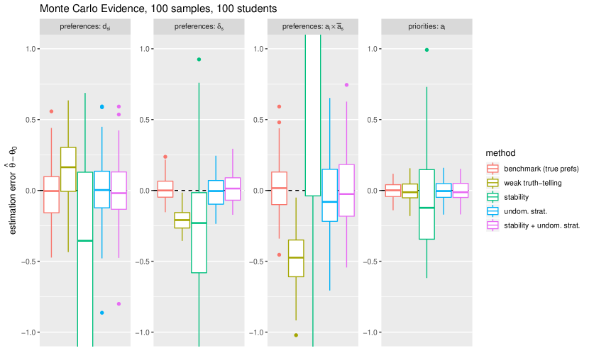
Figure A1: Distributions of estimation errors across one hundred simulated markets (six schools with 95 seats and 100 students).

(a) Mean squared error (MSE)

	preferences			priorities
method	$d_{is}$	$\delta_{s}$	$a_{i}\cdot\bar{a}_{s}$	$a_{i}$
benchmark (true prefs.)	0.0393	0.0065	0.0391	0.0028
weak truth–telling	0.0643	0.0496	0.2832	0.0048
stability	4.7436	0.3016	28.3876	0.1974
undominated strategies	0.0547	0.0114	0.0801	0.0049
stability + undom. strat.	0.0517	0.0107	0.0798	0.0047

(b) Bias

	preferences			priorities
method	$d_{is}$	$\delta_{s}$	$a_{i}\cdot\bar{a}_{s}$	$a_{i}$
benchmark (true prefs.)	-0.0144	0.0091	0.0223	0.0001
weak truth–telling	0.1498	-0.2091	-0.4897	-0.0050
stability	-1.0446	-0.2945	3.0821	-0.0283
undominated strategies	-0.0016	-0.0073	-0.0323	0.0003
stability + undom. strat.	-0.0213	0.0146	0.0093	0.0011

Table A1: MSE and bias statistics for one hundred simulated markets (six schools with 95 seats and 100 students).

500 students

The variance of the estimates improves considerably in larger markets, as figure A2 below shows. However, the stability based estimator still produces estimates that are rather imprecise, and also biased.

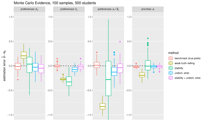
Figure A2: Distributions of estimation errors across one hundred simulated markets (six schools with 475 seats and 500 students).

(a) Mean squared error (MSE)

	preferences			priorities
method	$d_{is}$	$\delta_{s}$	$a_{i}\cdot\bar{a}_{s}$	$a_{i}$
benchmark (true prefs.)	0.0083	0.0016	0.0093	0.0010
weak truth–telling	0.0549	0.0743	0.6863	0.0398
stability	0.0446	0.1207	0.3576	0.0328
undominated strategies	0.0158	0.0086	0.0343	0.0015
stability + undom. strat.	0.0163	0.0035	0.0217	0.0016

(b) Bias

	preferences			priorities
method	$d_{is}$	$\delta_{s}$	$a_{i}\cdot\bar{a}_{s}$	$a_{i}$
benchmark (true prefs.)	-0.0129	-0.0019	0.0152	-0.0208
weak truth–telling	0.2179	-0.2704	-0.8242	-0.1892
stability	0.0141	-0.3243	-0.2801	0.0242
undominated strategies	-0.0207	-0.0726	-0.1198	-0.0181
stability + undom. strat.	-0.0515	-0.0238	-0.0404	-0.0172

Table A2: MSE and bias statistics for one hundred simulated markets (six schools with 475 seats and 500 students).

B.4 Data sources and construction

Since the data that we use contain very sensitive information, we had no direct access to it but instead let submitted our code to the Hungarian Education Authority (HEA) who executed it on their local computes. In order to develop our estimation routines, we were able to use an example dataset that closely resembled the actual data structure. This appendix is intended to provide some more information on the construction of our working data set.

Table A3 shows summary statistics of the student-level NABC data. Most students are fifteen years old at the time of the NABC test (in 2015). The NABC scores in Hungarian and mathematics are the results of a standardized test procedure. The socio-economic status (SES) is a composite measure that is based on responses given by students in an accompanying survey, so that this variable has more missing data. Also, the grade average is based on student’s own responses and may thus be biased. Therefore, we use the NABC scores as a proxy for student’s academic ability.

statistic	mean	SD	min	max	N
Birth year	2000.1	0.58216	1996	2002	88,959
Female	0.494	0.5	0	1	88,967
Last grade average	3.9837	0.7668	1	5	60,843
NABC score Hungarian	1559.9	202.36	820.97	2199.2	82,237
NABC score math	1612.1	196.5	907.81	2307.3	82,176
Socioeconomic status (csh)	-0.0226	1.01	-3.15	1.88	64,971

Table A3: Summary statistics of the original NABC (2015) data

Table A4 shows that there are significant differences in test outcomes and between male and female students. Female students perform much better in Hungarian on average (almost one third of a standard deviation), whereas male students perform better in math on average (one tenth of a standard deviation). Also, female students obtain a slightly better SES index (five percent of a standard deviation) but notice that the SES index is based on self reporting, so it could be due to different reporting behaviour. In all cases, the differences in means are significant at the one percent level.

	mean				t-test
statistic	all	male	female		diff.	t	p
NABC score Hungarian	1,560	1,538	1,583		-45.04	-32.109	$<$0.001
NABC score math	1,612	1,621	1,603		18.89	13.793	$<$0.001
Socioeconomic status (csh)	-0.023	-0.037	-0.008		-0.029	-3.644	$<$0.001

Table A4: Gender differences in test outcomes. Raw NABC (2015) data. Two-sample t-test with equal variance.

Table A5 shows key statistics of the nation-wide matching scheme. The data comprises almost four hundred thousand applications from almost ninety thousand students to over six thousand school programs. Each record corresponds to the application of a student to a school and contains the ranks $rk_{t}(s)$ and $rk_{s}(t)$, an indicator whether the school finds the student acceptable, and a match indicator. On average, each student applies to 4.5 school programs, or to 2.8 different schools. Almost 95% of all students are assigned to a school, of which three quarters are eventually assigned to their top choice program. We link this data to a school survey in order to obtain the precise location of each school, and the school’s district.

# students	$88,401$
# school programs	$6,181$
# schools (OMid-telephely-tipus)	$1,793$
# student-school applications	$395,222$
length of submitted ROL (school programs)	$4.471$
length of submitted ROL (schools)	$3.002$
# assigned	$83,482$
.. share top choice	$0.759$
.. average match rank	$1.486$

Table A5: Summary statistics of the original application data (KIFIR)

The HEA used a confidential concordance table to link records from the KIFIR and NABC datasets. As described in the main text, we restricted the linked sample to students who applied to at least one school from Budapest, which leaves us with 10,088 students.

As table A3 shows, the NABC scores and, in particular, the SES are missing for a quite substantial share of our sample. Because the computation of the student-optimal stable matching depends on the composition of the student sample, we were reluctant to drop records with missing data, as this would have left us with rather few complete records. Instead, we opted for a data imputation approach and used the R package mice to construct a complete dataset. Missing variables were imputed using predictive mean matching, were missing values are replaced by actual values from other records that resemble the incomplete record, conditional on other observed characteristics. As predictors, we used an extended set of variables that included also some results from the 2017 NABC round (where available), and further student level variables that are not shown here. This procedure is repeated a few times, until the imputed values converge in expectation. It is recommended that researchers construct multiple imputed datasets to assess the robustness of their analysis with respect to these imputations, but due to the substantial computational burden of our estimation procedures, this was infeasible in our context. The following table A6 shows details of the imputation procedure. It can be seen that the imputed mean of the variables referring to academic ability is lower than in the original data. Our imputation procedure naturally introduces measurement error into the data, which, in a classical regression framework, should lead to estimated coefficients that biased towards zero. We expect that this is also true for our estimation procedure which is, comprises a data augmentation approach with a linear regression. Nevertheless, it is our opinion that the drawbacks of using an imputed data set are greatly outweighed by the benefit of having a comprehensive set of students for the estimation procedure (which relies on stability considerations, and thus, on the entirety of the student population) and for the counter-factual matches (which are more directly dependent on the entire student population).

	raw data			imputed data
statistic	N	mean	SD	N	mean	SD	p
Birth year	$10,879$	$2,000.06$	$0.55$	1	$2,001.00$	–	$0.09$
Sex (1=female,2=male)	$10,880$	$1.50$	$0.50$	0	–	–	–
Last grade average	$6,598$	$4.12$	$0.68$	4,282	$3.97$	$0.70$	$<0.01$
NABC score Hungarian	$9,934$	$1,659.63$	$183.87$	946	$1,612.10$	$192.57$	$<0.01$
NABC score math	$9,948$	$1,607.88$	$186.60$	932	$1,569.42$	$189.95$	$<0.01$
Socioeconomic status (SES)	$7,097$	$0.45$	$0.87$	3,783	$0.41$	$0.88$	$0.02$

Table A6: Results of the imputation procedure, using predictive mean matching and ten iterations. The p-value is computed for a two-sided t-test with unequal variances.

In order to ease the interpretation of estimated preference parameters, we decided to standardize the NABC scores and the SES index to having a mean of zero, and unit standard deviation. This is shown in table 1 in the main text.

B.5 Decomposing the gains from consolidation: details

This section presents in detail how we construct the decomposition of the students’ consolidation gains into a choice effect and a competition effect. In doing so, we make use of the large market approximation to matching markets (Azevedo and Leshno, 2016) by which school-specific cutoff scores play the role of prices that balance the supply of, and the demand for school seats. The cutoff score at school $s$ under the matching $\mu$ is the lowest valuation among all students who where admitted to that school under $\mu$, or

$$c_{s}(\mu)=\min_{t\in\mu(s)}V_{s}(t)$$

We assume that the school market consists of relatively few schools and a large number of students so that the addition (or deletion) of a single student has practically no effect on a schools’ cutoff score, in line with the framework Azevedo and Leshno (2016). In order to decompose the total consolidation gains, we compute the school-level cutoff scores under the district wise matching $\mu_{d}$ and under the integrated matching $\mu_{BP}$. The effect of increased choice, keeping everything else constant, can then be computed as the difference between student $t$ being matched to her most preferred feasible school in her own district, and globally, using either the district-level or the city-wide cutoffs. Let the feasible set of student $t$ under the cutoffs $\{c_{s}(\mu)\}_{s\in S}$ be

$$\mathcal{F}_{t}^{\mu}=\left\{s\in S:V_{s}(t)\geq c_{s}(\mu)\right\}$$

and denote the set of schools in district $d$ as $S^{d}$. Then, the choice gain of student $t$ can either be expressed as

$$\Delta^{ch-I}U_{t}=\max_{s\in\mathcal{F}_{t}^{\mu_{BP}}}U_{t}(s)-\max_{s\in\mathcal{F}_{t}^{\mu_{BP}}\cap S^{d}}U_{t}(s)$$

or

$$\Delta^{ch-II}U_{t}=\max_{s\in\mathcal{F}_{t}^{\mu_{d}}}U_{t}(s)-\max_{s\in\mathcal{F}_{t}^{\mu_{d}}\cap S^{d}}U_{t}(s)$$

as is illustrated in figure 10. The only difference between $\Delta^{ch-I}U_{t}$ and $\Delta^{ch-II}U_{t}$ is the usage of a different baseline scenario to compute the cutoffs – the global cutoffs $\{c_{s}(\mu_{BP})\}$ for $\Delta^{ch-I}U_{t}$ and the local cutoffs for $\Delta^{ch-II}U_{t}$. It is easy to see that the choice gains will always be weakly positive by construction. It can also happen that a student is not assigned in one of the counter-factual scenarios. In our empirical application, the choice gains $\Delta^{ch-I}U_{t}$ are missing for about one quarter of all students, because their set of feasible schools within their home district is empty under the global cutoff scores. In a similar manner, one can compute the change in student $t$’s welfare as the market is opened up to external competition. We call this change a competition gain, but it is not a priori clear whether students actually gain or lose from competition. The competition gain can be computed either as

$$\Delta^{co-I}U_{t}=\max_{s\in\mathcal{F}_{t}^{\mu_{BP}}\cap S^{d}}U_{t}(s)-\max_{s\in\mathcal{F}_{t}^{\mu_{d}}\cap S^{d}}U_{t}(s)$$

or as

$$\Delta^{co-II}U_{t}=\max_{s\in\mathcal{F}_{t}^{\mu_{BP}}}U_{t}(s)-\max_{s\in\mathcal{F}_{t}^{\mu_{d}}}U_{t}(s)$$

Now, $\Delta_{t}^{co-I}$ differs from $\Delta^{co-II}U_{t}$ in that student $t$’s choice set is restricted to feasible schools within her home district $d$ in the former, but not in the latter. It is easy to see that the sum of $\Delta^{ch-I}U_{t}$ and $\Delta^{co-I}U_{t}$ is identical to the sum of $\Delta^{ch-II}U_{t}$ and $\Delta^{co-II}U_{t}$ unless some type-I choice gains are missing. Also, the sum of the choice and competition gains are equal to the total welfare gains.

B.6 Balanced markets

The Hungarian school market is characterized by a great amount of nominal excess capacity. To see whether, and if so, how, this affects the conclusions drawn in the main text, we repeated the analysis in section 6.3 with an artificially balanced market. This was achieved by scaling the schools’ capacities proportionally within each district until the total number of seats equals the total number of students (up to the integer constraint). In doing so, we guarantee that every student is matched to some school. Of course, this is a highly artificial setting, but it serves as a useful comparison benchmark against which the results from the main text can be viewed.

Table 7(a) shows the match statistics for the balanced markets. The consolidation gains were computed analogue to the main text. The first row of table 7(b) shows that the consolidation gains are now very small compared to the large gains achieved in the unbalanced markets, and the median student neither gains nor looses due to district consolidation. The de-composition into choice and competition effects, also shown in table 7(b), shows why this is the case: The choice, and the competition effects now have about equal magnitudes and opposite signs, and so they cancel each other. Interestingly, the competition effects are now strictly negative.

district markets
# matched	10,880
share top choice match	0.57
ave. match distance [km]	3.53
consolidated market
# matched	10,880
share top choice match	0.54
share matched in home district	0.18
ave. match distance [km]	8.99

(a) Assignment statistics of the district-wise and integrated student-school matching.

	Mean	SD	Min	Median	Max	N
total gains
in latent utility units	0.033	1.131	-7.000	0.000	5.000	10,880
in equivalent kilometres	0.223	7.639	-47.297	0.000	33.784	10,880
decomposition
choice effect I	1.190	1.203	0.000	0.929	7.445	7,536
competition effect I	-1.055	1.289	-8.060	-0.566	0.000	7,536
choice effect II	1.050	0.981	0.000	0.888	6.725	10,880
competition effect II	-1.017	0.818	-6.791	-0.924	0.000	10,880

(b) Various measures of consolidation gains, expressed in latent utility changes.

Table A7: Gains from market consolidation using inferred complete preferences lists and artificially balanced markets: summary statistics

Figure 3(a) shows that there is a weakly negative relationship between ex post majority support for market consolidation and district size. A linear regression analysis (not shown here) confirms this, but does not find a significant effect ($p=0.139$). The important difference to result from the main text, which were derived with the original amount of excess capacity, not all districts have a majority of consolidation winners. Figure 3(b) shows that there is a weakly negative correlation between average latent utility gains and district size, similar to figure 9(a). Again, this negative effect is insignificant in a linear model ($p=0.448$). Thus, we cannot confirm the prediction of Corollary 1 in this case. Because all district-level school markets were exactly balanced in this exercise, it is not possible to determine how the excess capacity affects the gains from consolidation.

We also estimated a linear regression of the students’ total gain and their choice and competition gains on student and district observables, the results of which are shown in table A8. Contrary to table 13, students with a higher SES gain less than the average student, but the coefficient is equally insignificant. Furthermore, high-ability students have significantly larger consolidation gains. Interestingly, the estimated effect of a student’s home district size is now significantly positive, contrary to the correlation in figure 3(b). However, when the district FEs are not included (results not shown here), the effect is significantly negative.

In conclusion, this appendix shows that the results from the main text do not necessarily carry over to situations where the aggregate school market has less excess capacity or is even balanced. With artificially balanced markets, the median student neither gains nor losses due to market consolidation, and the share of students who gain is below fifty percent in many districts. This is somewhat at odds with the theoretical predictions in chapter 3 where we showed that the expected consolidation gains are positive for students in all districts (Corollary 1), and it could be due to the fact that those theoretical results were derived under the assumption of uniform and random preferences. Therefore, it seems imperative for theoretical researchers to extend the set of possible preference structures that are accommodated by their models.

(a) Share of winners and district sizes

(b) Average latent utility gains and district sizes

Figure A3: Majority support for, and average latent utility gains of market consolidation, using inferred complete preference lists and balanced markets.

	Dependent variable: latent utility gains
		type-I decomposition		type-II decomposition
	total	choice	competition	choice	competition
	(1)	(2)	(3)	(4)	(5)
socio-economic status SES	-0.0099	0.0585∗∗∗	-0.0716∗∗∗	0.0494∗∗∗	-0.0594∗∗∗
	-0.0121	-0.0164	-0.017	-0.0106	-0.0091
ability	0.0839∗∗∗	0.0404∗∗∗	0.0235∗	0.0066	0.0772∗∗∗
	-0.0088	-0.0123	-0.0127	-0.0077	-0.0066
district size (100 students)	0.2044∗∗∗	-0.1431	0.2173	0.0203	0.1841∗∗∗
	-0.0559	-0.1533	-0.1587	-0.0492	-0.042
school type: gymnazium	0.0993∗∗∗	0.0854∗∗	-0.0089	-0.0193	0.1186∗∗∗
	-0.0295	-0.0424	-0.0438	-0.0259	-0.0222
school type: secondary	-0.5061∗∗∗	1.4227∗∗∗	-1.4857∗∗∗	1.3117∗∗∗	-1.8178∗∗∗
	-0.1579	-0.4762	-0.4928	-0.1388	-0.1186
Constant	-0.5061∗∗∗	1.4227∗∗∗	-1.4857∗∗∗	1.3117∗∗∗	-1.8178∗∗∗
	-0.1579	-0.4762	-0.4928	-0.1388	-0.1186
district FE	Yes	Yes	Yes	Yes	Yes
Observations	10,880	7,536	7,536	10,880	10,880
Note:	∗p$<$0.1; ∗∗p$<$0.05; ∗∗∗p$<$0.01
	Standard errors in parentheses.

Table A8: Explaining gains from consolidation with students observables (balanced markets). The table shows regression coefficients of students’ gains on student observables. The school type refers to the school type of the assigned school in the integrated market.

References

- Abdulkadiroğlu et al. (2017) Abdulkadiroğlu, A., N. Agarwal, and P. A. Pathak (2017): “The welfare effects of coordinated assignment: Evidence from the New York City high school match,” American Economic Review, 107, 3635–89.
- Abdulkadiroğlu et al. (2014) Abdulkadiroğlu, A., J. Angrist, and P. Pathak (2014): “The elite illusion: Achievement effects at Boston and New York exam schools,” Econometrica, 82, 137–196.
- Abdulkadiroğlu and Sönmez (2003) Abdulkadiroğlu, A. and T. Sönmez (2003): “School choice: A mechanism design approach,” American Economic Review, 93, 729–747.
- Agarwal (2015) Agarwal, N. (2015): “An empirical model of the medical match,” American Economic Review, 105, 1939–78.
- Agarwal and Diamond (2014) Agarwal, N. and W. Diamond (2014): “Identification and estimation in two-sided matching markets,” Cowles foundation discussion papers, Yale University.
- Akyol and Krishna (2017) Akyol, P. and K. Krishna (2017): “Preferences, selection, and value added: A structural approach,” European Economic Review, 91, 89–117.
- Albert and Chib (1993) Albert, J. H. and S. Chib (1993): “Bayesian analysis of binary and polychotomous response data,” Journal of the American Statistical Association, 88, 669–679.
- Alsbury and Shaw (2005) Alsbury, T. and N. Shaw (2005): “Policy implications for social justice in school district consolidation,” Leadership and Policy in Schools, 4, 105–126.
- Artemov et al. (2017) Artemov, G., Y.-K. Che, and Y. He (2017): “Strategic ‘mistakes’: Implications for market design research,” NBER Working Paper.
- Ashlagi et al. (2017) Ashlagi, I., Y. Kanoria, and J. Leshno (2017): “Unbalanced random matching markets: The stark effect of competition,” Journal of Political Economy, 125, 69–98.
- Azevedo and Leshno (2016) Azevedo, E. M. and J. D. Leshno (2016): “A supply and demand framework for two-sided matching markets,” Journal of Political Economy, 124, 1235–1268.
- Baswana et al. (2019) Baswana, S., P. P. Chakrabarti, S. Chandran, Y. Kanoria, and U. Patange (2019): “Centralized admissions for engineering colleges in India,” Interfaces, 49, 338–354.
- Beggs et al. (1981) Beggs, S., S. Cardell, and J. Hausman (1981): “Assessing the potential demand for electric cars,” Journal of Econometrics, 17, 1 – 19.
- Berry (2005) Berry, C. R. (2005): “School district consolidation and student outcomes: Does size matter?” in Besieged: School Boards and the Future of Education Politics, ed. by W. G. Howell, Brookings Institution Press Washington, DC, 56–80.
- Berry and West (2008) Berry, C. R. and M. R. West (2008): “Growing pains: The school consolidation movement and student outcomes,” The Journal of Law, Economics, & Organization, 26, 1–29.
- Biró (2008) Biró, P. (2008): “Student admissions in Hungary as Gale and Shapley envisaged,” Tech. rep., University of Glasgow.
- Biró (2012) ——— (2012): “Matching practices for secondary schools – Hungary,” Tech. rep., MiP Country Profile 6.
- Brasington (1999) Brasington, D. M. (1999): “Joint provision of public goods: the consolidation of school districts,” Journal of Public Economics, 73, 373 – 393.
- Braun et al. (2010) Braun, S., N. Dwenger, and D. Kübler (2010): “Telling the truth may not pay off: An empirical study of centralized university admissions in Germany,” The BE Journal of Economic Analysis & Policy, 10.
- Bucarey (2018) Bucarey, A. (2018): “Who pays for free college? Crowding out on campus,” Tech. rep., MIT.
- Bukodi et al. (2008) Bukodi, E., P. Róbert, and S. Altorjai (2008): “The Hungarian educational system and the implementation of the ISCED-97,” The International Standard Classification of Education, 200–215.
- Burgess et al. (2015) Burgess, S., E. Greaves, A. Vignoles, and D. Wilson (2015): “What parents want: School preferences and school choice,” The Economic Journal, 125, 1262–1289.
- Cameron and Trivedi (2005) Cameron, A. C. and P. K. Trivedi (2005): Microeconometrics: Methods and Applications, Cambridge University Press.
- Castillo and Dianat (2016) Castillo, M. and A. Dianat (2016): “Truncation strategies in two-sided matching markets: Theory and experiment,” Games and Economic Behavior, 98, 180–196.
- Chade et al. (2014) Chade, H., G. Lewis, and L. Smith (2014): “Student portfolios and the college admissions problem,” Review of Economic Studies, 81, 971–1002.
- Che and Koh (2016) Che, Y.-K. and Y. Koh (2016): “Decentralized college admissions,” Journal of Political Economy, 124, 1295–1338.
- Che and Tercieux (2019) Che, Y.-K. and O. Tercieux (2019): “Efficiency and stability in large matching markets,” Journal of Political Economy, 127, 2301–2342.
- Chen (2013) Chen, J. (2013): “Estimation of the loan spread equation with endogenous bank-firm matching,” Advances in Econometrics, 3, 251–289.
- Chen and Pereyra (2019) Chen, L. and J. S. Pereyra (2019): “Self-selection in school choice,” Games and Economic Behavior, 117, 59 – 81.
- Correa et al. (2019) Correa, J., R. Epstein, J. Escobar, I. Rios, B. Bahamondes, C. Bonet, N. Epstein, N. Aramayo, M. Castillo, A. Cristi, et al. (2019): “School choice in Chile,” in Proceedings of the 2019 ACM Conference on Economics and Computation, 325–343.
- Cox (2010) Cox, B. (2010): “A decade of results: a case for school district consolidation?” Education, 131, 83–92.
- Doğan and Yenmez (2017) Doğan, B. and B. Yenmez (2017): “Unified enrollment in school choice: How to improve student assignment in Chicago,” Tech. rep., SSRN preprint.
- Duncombe et al. (1995) Duncombe, W., J. Miner, and J. Ruggiero (1995): “Potential cost savings from school district consolidation: A case study of New York,” Economics of Education Review, 14, 265–284.
- Ekmekci and Yenmez (2019) Ekmekci, M. and B. Yenmez (2019): “Common enrollment in school choice,” Theoretical Economics, 14, 1237–1270.
- Fack et al. (2019) Fack, G., J. Grenet, and Y. He (2019): “Beyond truth-telling: Preference estimation with centralized school choice and college admissions,” American Economic Review, 109, 1486–1529.
- Fairman and Donis-Keller (2012) Fairman, J. C. and C. Donis-Keller (2012): “School district reorganization in Maine: Lessons learned for policy and process,” Maine Policy Review, 21, 24–40.
- Fernandez and Rodrik (1991) Fernandez, R. and D. Rodrik (1991): “Resistance to reform: Status quo bias in the presence of individual- specific uncertainty,” American Economic Review, 81, pp. 1146–1155.
- Gale and Shapley (1962) Gale, D. and L. S. Shapley (1962): “College admissions and the stability of marriage,” The American Mathematical Monthly, 69, 9–15.
- Gordon and Knight (2009) Gordon, N. and B. Knight (2009): “A spatial merger estimator with an application to school district consolidation,” Journal of Public Economics, 93, 752–765.
- Haeringer and Klijn (2009) Haeringer, G. and F. Klijn (2009): “Constrained school choice,” Journal of Economic Theory, 144, 1921–1947.
- Hafalir et al. (2019) Hafalir, I., F. Kojima, and B. Yenmez (2019): “Interdistrict school choice: A theory of student assignment,” Tech. rep., SSRN preprint.
- Hafalir and Yenmez (2017) Hafalir, I. and B. Yenmez (2017): “Integrating school districts: Diversity, balance, and welfare,” Tech. rep., SSRN preprint.
- Hafalir et al. (2018) Hafalir, I. E., R. Hakimov, D. Kübler, and M. Kurino (2018): “College admissions with entrance exams: Centralized versus decentralized,” Journal of Economic Theory, 176, 886 – 934.
- Hastings et al. (2013) Hastings, J. S., C. A. Neilson, and S. D. Zimmerman (2013): “Are some degrees worth more than others? Evidence from college admission cutoffs in Chile,” NBER Working Paper.
- He and Magnac (2019) He, Y. and T. Magnac (2019): “Application Costs and Congestion in Matching Markets,” Tech. rep., Toulouse School of Economics.
- Hiller and Tercieux (2014) Hiller, V. and O. Tercieux (2014): “Choix d’écoles en France,” Revue Économique, 65, 619–656.
- Howley et al. (2011) Howley, C., J. Johnson, and J. Petrie (2011): “Consolidation of schools and districts: What the research says and what it means,” National Education Policy Center.
- Kertesi and Kézdi (2013) Kertesi, G. and G. Kézdi (2013): “School segregation, school choice, and educational policies in 100 Hungarian towns,” Tech. rep., Corvinus University Budapest.
- Kirkebøen (2012) Kirkebøen, L. (2012): “Preferences for lifetime earnings, earnings risk and nonpecuniary attributes in choice of higher education,” Statistics Norway Discussion Paper 725.
- Kumar et al. (2020) Kumar, R., K. Manocha, and J. Ortega (2020): “On the integration of Shapley-Scarf housing markets,” arXiv preprint arXiv:2004.09075.
- Lancaster (2004) Lancaster, T. (2004): An Introduction to Modern Bayesian Econometrics, Blackwell.
- Leach et al. (2010) Leach, J., A. A. Payne, and S. Chan (2010): “The effects of school board consolidation and financing on student performance,” Economics of Education Review, 29, 1034–1046.
- Logan et al. (2008) Logan, J. A., P. D. Hoff, and M. A. Newton (2008): “Two-sided estimation of mate preferences for similarities in age, education, and religion,” Journal of the American Statistical Association, 103, 559–569.
- Luxen and Vetter (2011) Luxen, D. and C. Vetter (2011): “Real-time routing with OpenStreetMap data,” in Proceedings of the 19th ACM SIGSPATIAL International Conference on Advances in Geographic Information Systems, 513–516.
- Machado and Szerman (2018) Machado, C. and C. Szerman (2018): “Centralized admissions and the student-college match,” Tech. rep., SSRN preprint.
- Manjunath and Turhan (2016) Manjunath, V. and B. Turhan (2016): “Two school systems, one district: What to do when a unified admissions process is impossible,” Games and Economic Behavior, 95, 25–40.
- McGill et al. (1978) McGill, R., J. W. Tukey, and W. A. Larsen (1978): “Variations of box plots,” The American Statistician, 32, 12–16.
- Menzel (2015) Menzel, K. (2015): “Large matching markets as two-sided demand systems,” Econometrica, 83, 897–941.
- Menzel and Salz (2013) Menzel, K. and T. Salz (2013): “Robust decisions with incomplete structural models of strategic interactions,” Tech. rep., New York University.
- Mora and Romero-Medina (2001) Mora, R. and A. Romero-Medina (2001): “Understanding preference formation in a matching market,” Tech. rep., Universidad Carlos III de Madrid.
- Ortega (2018) Ortega, J. (2018): “Social integration in two-sided matching markets,” Journal of Mathematical Economics, 78, 119 – 126.
- Ortega (2019) ——— (2019): “The losses from integration in matching markets can be large,” Economics Letters, 174, 48 – 51.
- Riedel et al. (2010) Riedel, A., K. Schneider, C. Schuchart, and H. Weishaupt (2010): “School choice in German primary schools. How binding are school districts?” Journal for Educational Research Online, 2, 94–120.
- Roth and Sotomayor (1992) Roth, A. and M. Sotomayor (1992): Two-sided matching: A study in game-theoretic modeling and analysis, Econometric Society Monographs, Cambridge University Press.
- Siegel-Hawley et al. (2017) Siegel-Hawley, G., K. Bridges, and T. J. Shields (2017): “Solidifying segregation or promoting diversity? School closure and rezoning in an urban district,” Educational Administration Quarterly, 53, 107–141.
- Söderström and Uusitalo (2010) Söderström, M. and R. Uusitalo (2010): “School choice and segregation: evidence from an admission reform,” Scandinavian Journal of Economics, 112, 55–76.
- Sørensen (2007) Sørensen, M. (2007): “How smart is smart money? A two-sided matching model of venture capital,” The Journal of Finance, 62, 2725–2762.
- Sprumont (1990) Sprumont, Y. (1990): “Population monotonic allocation schemes for cooperative games with transferable utility,” Games and Economic Behavior, 2, 378–394.
- Tamer (2003) Tamer, E. (2003): “Incomplete simultaneous discrete response model with multiple equilibria,” Review of Economic Studies, 70, 147–165.
- Train (2009) Train, K. E. (2009): Discrete Choice Methods with Simulation, Cambridge University Press, 2 ed.
- Turhan (2019) Turhan, B. (2019): “Welfare and incentives in partitioned school choice markets,” Games and Economic Behavior, 113, 199–208.
- van Buuren and Groothuis-Oudshoorn (2011) van Buuren, S. and K. Groothuis-Oudshoorn (2011): “mice: Multivariate Imputation by Chained Equations in R,” Journal of Statistical Software, 45, 1–67.
- Waslander and Thrupp (1995) Waslander, S. and M. Thrupp (1995): “Choice, competition and segregation: an empirical analysis of a New Zealand secondary school market, 1990-93,” Journal of Education Policy, 10, 1–26.
- Weldon (2016) Weldon, M. (2016): “School Choice, Competition and Ethnic Segregation in Lancashire: Evidence from structural models of two-sided matching,” Ph.D. thesis.
- Wilson (1972) Wilson, L. (1972): “An analysis of the stable marriage assignment algorithm,” BIT Numerical Mathematics, 12, 569–575.
- Yao and Böckenholt (1999) Yao, G. and U. Böckenholt (1999): “Bayesian estimation of Thurstonian ranking models based on the Gibbs sampler,” British Journal of Mathematical and Statistical Psychology, 52, 79–92.