A stabilized finite element method for inverse problems subject to the convection–diffusion equation. II: convection-dominated regime

Abstract.

We consider the numerical approximation of the ill-posed data assimilation problem for stationary convection–diffusion equations and extend our previous analysis in [Numer. Math. 144, 451–477, 2020] to the convection-dominated regime. Slightly adjusting the stabilized finite element method proposed for dominant diffusion, we draw upon a local error analysis to obtain quasi-optimal convergence along the characteristics of the convective field through the data set. The weight function multiplying the discrete solution is taken to be Lipschitz continuous and a corresponding super approximation result (discrete commutator property) is proven. The effect of data perturbations is included in the analysis and we conclude the paper with some numerical experiments.

1. Introduction

In this work, we consider a data assimilation problem for a stationary convection–diffusion equation

(1) $$\mathcal{L}u:=-\mu\Delta u+\beta\cdot\nabla u=f\quad\text{in }\Omega\subset\mathbb{R}^{n},$$

when convection dominates, that is $0<\mu\ll|\beta|$, and complement the diffusion-dominated case discussed in the first part [BNO20]. We assume that $\Omega\subset\mathbb{R}^{n}$ is open, bounded and connected, and there exists a solution $u\in H^{2}(\Omega)$ to (1). The problem under study is to approximate the solution $u$ given the source $f$ in $\Omega$ and the perturbed restriction $\tilde{U}_{\omega}=u|_{\omega}+\delta$ of the solution to an open subset $\omega\subset\Omega$. The perturbation $\delta$ is taken in $L^{2}(\omega)$. Notice that we consider no boundary conditions on $\partial\Omega$. This is a linear ill-posed problem also known as unique continuation.

To start with, let us briefly recall the main results obtained in the first part. Consider an open bounded set $B\subset\Omega$ that contains the data region $\omega$ such that $B\setminus\omega$ does not touch the boundary of $\Omega$. For $u\in H^{1}(\Omega)$, the following conditional stability estimate was proven for $\mu>0$ and $\beta\in L^{\infty}(\Omega)^{n}$,

(2) $$\left\|u\right\|_{L^{2}(B)}\leq C_{st}\left(\left\|u\right\|_{L^{2}(\omega)}+\tfrac{1}{\mu}\left\|\mathcal{L}u\right\|_{H^{-1}(\Omega)}\right)^{\kappa}\left\|u\right\|_{L^{2}(\Omega)}^{1-\kappa},$$

where the Hölder exponent $\kappa\in(0,1)$ depends only on the geometric setting. In the case of simple geometric configurations, e.g. when $\omega,\,B,\,\Omega$ are three concentric balls, the exponent $\kappa\in(0,1)$ can be given explicitly, see [BNO20, Remark 1]. The stability constant $C_{st}$ is given explicitly in terms of the physical parameters

(3) $$C_{st}=C_{1}\exp\left(C_{2}(1+\tfrac{|\beta|}{\mu})^{2}\right),\quad|\beta|:=\left\|\beta\right\|_{L^{\infty}(\Omega)^{n}},$$

with constants $C_{1},\,C_{2}>0$ depending only on the geometry. Note that the continuum estimate (2) is valid in both the diffusion-dominated and convection-dominated regimes, and that the stability constant $C_{st}$ is uniformly bounded when diffusion dominates. However, when convection dominates $C_{st}$ grows exponentially, rendering the stability estimate ineffective in practice. We also recall that for global unique continuation from $\omega$ to the entire $\Omega$ the stability is no longer Hölder, but logarithmic, that is the modulus of continuity for the given data is not $|\cdot|^{\kappa}$ any more, but $|\log(\cdot)|^{-\kappa}$.

On the discrete level, the continuum estimate (2) was combined with a stabilized linear finite element method to obtain convergence orders for the approximate solution. More precisely, for a mesh size $h$, and defining the Péclet number

$$Pe(h):=\frac{|\beta|h}{\mu},$$

the following error bound [BNO20, Theorem 1] was proven for the approximation $u_{h}$ in the diffusive regime $Pe(h)<1$,

(4) $$\|u-u_{h}\|_{L^{2}(B)}\leq C_{st}\,h^{\kappa}(\|u\|_{H^{2}(\Omega)}+h^{-1}\|\delta\|_{L^{2}(\omega)}),$$

where the convergence order $\kappa\in(0,1)$ is the same as the Hölder exponent in (2) and the stability constant $C_{st}$ is proportional to the one in (3). Under an additional assumption on the divergence of the convective field $\beta$, similar error bounds were also proven in the $H^{1}$-norm, see [BNO20, Theorem 2].

The prototypical effect of dominating diffusion is shown in Figure 1, where the problem is set in the unit square and contour error plots are shown for data assimilation from a centered disk of radius 0.1. One can notice oscillating errors that grow in size away from the data region towards the boundary. The exact solution in this example is $u=2\sin(5\pi x)\sin(5\pi y)$ where the factor 2 is taken to make its $L^{2}$-norm unitary. For the computation we used an unstructured mesh with 512 elements on a side and mesh size $h\approx 0.0025$.

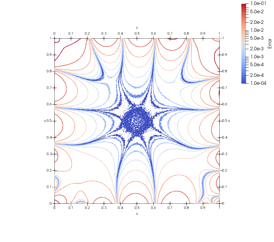
Figure 1. Absolute error contour plot in the diffusion-dominated case, $\mu=1,\,\beta=(1,0)$. The domain is the unit square, data given in a centered disk of radius 0.1 for the exact solution $u=2\sin(5\pi x)\sin(5\pi y)$.

1.1. Objective and main results

We consider a stabilized finite element method for data assimilation subject to the convection–diffusion equation in the convection-dominated regime. Since the behaviour of the physical system changes fundamentally when convection dominates and

$$Pe(h)\gg 1,$$

the goal of this second part paper is to reconsider the numerical method proposed in the first part [BNO20] and develop an error analysis that captures and exploits the governing transport phenomenon. This is illustrated in Figure 2 where the transition to the convection-dominated regime through an intermediate regime is made by decreasing the diffusion coefficient $\mu$. We aim to obtain sharper local error estimates along the characteristics of the convective field through the data region. Even though the error analysis that we perform herein is different in nature to the one in the first part, the numerical method itself is only slightly changed (see Remark 1 below). For the error localization technique we draw on ideas used for the streamline diffusion method in [JNP84], continuous interior penalty in [BGL09], and non-coercive hyperbolic problems in [Bur14].

From the definition of the Péclet number we see that the regime will also depend on the resolution of the computation besides the physical parameters. We can therefore expect the method to change behaviour as the resolution increases and $Pe(h)$ decreases. This phenomenon was already observed computationally in [Bur13] and can now be explained theoretically.

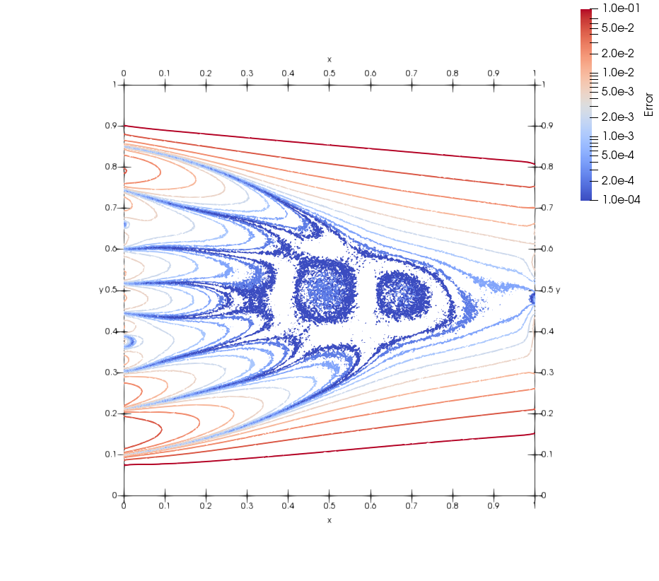
(a) $\mu=10^{-2}$.

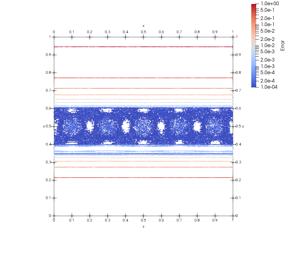
(b) $\mu=10^{-6}$.

Figure 2. Absolute error contour plot when convection becomes dominant, $\beta=(1,0)$. The domain is the unit square, data given in a centered disk of radius 0.1 for the exact solution $u=2\sin(5\pi x)\sin(5\pi y)$.

To make the presentation as simple as possible we consider a model case in the unit square $\Omega$ with constant convection

$$\beta:=(\beta_{1},0),\quad\beta_{1}\in\mathbb{R},$$

and the solution given in the subset

$$\omega:=(0,x)\times(y^{-},y^{+})\text{ with }x>h\text{ and }y^{+}-y^{-}>h.$$

For the subset ${\omega_{\beta}}\subset\Omega$ covered by the characteristics of $\beta$ that go through $\omega$, we introduce the stability region ${\mathring{\omega}_{\beta}}\subset\omega_{\beta}$ by cutting off a crosswind layer of width $\mathcal{O}(h^{\frac{1}{2}}|\ln(h)|)$ (see Section 2.1 for more details). We separate the convection-dominated and diffusion-dominated regimes by introducing a constant $Pe_{\lim}>1$ such that

$$Pe(h)>Pe_{\lim}>1.$$

To reduce the number of constants appearing in the analysis, we will write this as $Pe(h)\gtrsim 1$. As suggested by Figure 2, we expect different results for data assimilation downstream vs upstream in an intermediate regime. We prove in Theorem 1 weighted error estimates that for $\beta_{1}>0$ essentially take the following form

$$\|u-u_{h}\|_{L^{2}(\mathring{\omega}_{\beta})}\leq C(|\beta|^{\frac{1}{2}}h^{\frac{3}{2}}|u|_{H^{2}(\Omega)}+|\beta|^{\frac{1}{2}}h^{-\frac{1}{2}}\|\delta\|_{L^{2}(\omega)}),\text{ when }Pe(h)\gtrsim 1.$$

This is similar to the typical error estimates for piecewise linear stabilized FEMs for convection-dominated well-posed problems, such as local projection stabilization, dG methods, continuous interior penalty or Galerkin least squares. On general shape-regular meshes these methods have an $\mathcal{O}(h^{\frac{1}{2}})$ gap to the best approximation convergence order. Taking this into account, our result is thus quasi-optimal. For a recent overview of challenges and open problems in the well-posed case, see e.g. [JKN18] and [RS15].

When going against the characteristics, i.e. $\beta_{1}<0$, we prove in Theorem 2 first the pre-asymptotic bound

$$\|u-u_{h}\|_{L^{2}(\mathring{\omega}_{\beta})}\leq C(|\beta|^{\frac{1}{2}}h|u|_{H^{2}(\Omega)}+h^{-1}\|\delta\|_{L^{2}(\omega)}),\text{ when }1\lesssim Pe(h)<h^{-1},$$

followed by

$$\|u-u_{h}\|_{L^{2}(\mathring{\omega}_{\beta})}\leq C(|\beta|^{\frac{1}{2}}h^{\frac{3}{2}}|u|_{H^{2}(\Omega)}+h^{-\frac{1}{2}}\|\delta\|_{L^{2}(\omega)}),\text{ when }Pe(h)>h^{-1}.$$

It follows that when solving the data assimilation problem against the flow, the diffusivity reduces the convergence order in an intermediate regime. Only for very small diffusion coefficients $\mu<|\beta|h^{2}$ do we get quasi-optimal bounds. This asymmetry of the error distribution for moderate Péclet numbers is clearly visible in the left plot of Figure 2.

Previous results on optimal control for stabilized convection–diffusion equations include [BV07, DQ05, HYZ09, YZ09]. We refer to the first part [BNO20] for a more detailed discussion.

In terms of notation, above and throughout the paper $C$ denotes a generic positive constant, not necessarily the same at each occurrence, that is independent of the coefficients $\mu,\,\beta$ and the mesh size $h$.

2. Discrete setting

Let $V_{h}\subset H^{1}(\Omega)$ be the conforming finite element space of piecewise affine $\mathbb{P}_{1}$ functions defined on a computational mesh $\mathcal{T}_{h}$ that consists of shape-regular triangular elements $K$ with diameter $h_{K}$. The mesh size $h$ is the maximum over $h_{K}$ and we will assume that $h<1$. The interior faces of all the elements are collected in the set $\mathcal{F}_{i}$ and the jump of a quantity across such a face $F$ is denoted by $\llbracket\cdot\rrbracket_{F}$, omitting the subscript whenever the context is clear. We denote by $n$ the unit normal.

First we introduce the standard inner products with the induced norms

$$(v_{h},w_{h})_{\Xi}:=\int_{\Xi}v_{h}w_{h}~{}\mbox{d}x,\quad\left<v_{h},w_{h}\right>_{\partial\Xi}:=\int_{\partial\Xi}v_{h}w_{h}~{}\mbox{d}s,$$

and the bilinear form in the weak formulation of (1)

$$a_{h}(v_{h},w_{h}):=(\beta\cdot\nabla v_{h},w_{h})_{\Omega}+(\mu\nabla v_{h},\nabla w_{h})_{\Omega}-\left<\mu\nabla v_{h}\cdot n,w_{h}\right>_{\partial\Omega}.$$

We will make use of the stabilizing bilinear forms

$$s_{\Omega}(v_{h},w_{h}):=\gamma\sum_{F\in\mathcal{F}_{i}}\int_{F}h(\mu+|\beta|h)\llbracket\nabla v_{h}\cdot n\rrbracket\cdot\llbracket\nabla w_{h}\cdot n\rrbracket~{}\mbox{d}s,$$

which will act on the discrete solution penalizing the jumps of its gradient across interior faces, and

$$s_{*}(v_{h},w_{h}):=\gamma_{*}\left(\left<(|\beta|+\mu h^{-1})v_{h},w_{h}\right>_{\partial\Omega}+(\mu\nabla v_{h},\nabla w_{h})_{\Omega}+s_{\Omega}(v_{h},w_{h})\right),$$

where $\gamma$ and $\gamma_{*}$ are positive constants that can be heuristically chosen at implementation. They do not play a role in the convergence of the method and most of the time we will include them in the generic constant $C$. For the data assimilation term we consider the scaled inner product in the data set $\omega$ given by

$$s_{\omega}(v_{h},w_{h}):=((|\beta|h^{-1}+\mu h^{-\zeta})v_{h},w_{h})_{\omega},\quad\zeta\in[0,2].$$

To this we add the stabilizing interior penalty term $s_{\Omega}$ to define for conciseness

$$s(v_{h},w_{h}):=s_{\Omega}(v_{h},w_{h})+s_{\omega}(v_{h},w_{h}),$$

The idea behind the computational method follows the discretize-then-optimize approach: we first discretize and then formulate the data assimilation problem as a PDE-constrained optimization problem with additional stabilizing terms. Apart from their stabilizing intake, these terms are also chosen such that they vanish at optimal rates. For an overview on this approach to ill-posed problems and more details on the desired properties of discrete stabilizers, we refer the reader to [Bur13]. To be more precise, for an approximation $u_{h}\in V_{h}$ and a discrete Lagrange multiplier $z_{h}\in V_{h}$, we consider the functional

$$L_{h}(u_{h},z_{h}):={} \tfrac{1}{2}s_{\omega}(u_{h}-\tilde{U}_{\omega},u_{h}-\tilde{U}_{\omega})+a_{h}(u_{h},z_{h})-(f,z_{h})_{\Omega}$$

$$+\tfrac{1}{2}s_{\Omega}(u_{h},u_{h})-\tfrac{1}{2}s_{*}(z_{h},z_{h}),$$

where the first term is measuring the misfit between $u_{h}$ and the known perturbed restriction $\tilde{U}_{\omega}=u|_{\omega}+\delta$, the next two terms are imposing the weak form of the PDE (1) as a constraint, and the last two terms have stabilizing role and act only on the discrete level.

We look for the saddle points of the Lagrangian $L_{h}$ and analyse their convergence to the exact solution. Using the optimality conditions we obtain the finite element method for data assimilation subject to (1), which reads as follows: find $(u_{h},z_{h})\in[V_{h}]^{2}$ such that

(5) $$\left\{\begin{array}[]{rcl}a_{h}(u_{h},w_{h})-s_{*}(z_{h},w_{h})&=&(f,w_{h})_{\Omega}\\ a_{h}(v_{h},z_{h})+s(u_{h},v_{h})&=&s_{\omega}(\tilde{U}_{\omega},v_{h})\end{array}\right.,\quad\forall(v_{h},w_{h})\in[V_{h}]^{2}.$$

Notice that the exact solution $u\in H^{2}(\Omega)$ (with noise $\delta\equiv 0$) and the dual variable $z\equiv 0$ satisfy (5) since the gradient of the exact solution has no jumps across interior faces. Hence the Lagrange multiplier $z_{h}$ should converge to zero.

Remark 1.

The same finite element method (5) has been proposed in the first part [BNO20] for the diffusion-dominated case; $s_{\Omega}$ and $s_{*}$ are exactly the stabilizing terms introduced there. However, herein we have increased the penalty coefficient in the data term $s_{\omega}$ from $|\beta|h+\mu$ to $|\beta|h^{-1}+\mu h^{-\zeta}$. We note that the bounds in [BNO20] hold also for this stronger penalty term, but the sensitivity to perturbations in data increases by a factor of $h^{-1}$.

Proposition 1.

The finite element method (5) has a unique solution $(u_{h},z_{h})\in[V_{h}]^{2}$ and the Euclidean condition number $\mathcal{K}_{2}$ of the system matrix satisfies

$$\mathcal{K}_{2}\leq Ch^{-4}.$$

Proof.

The proof given in [BNO20, Proposition 2] holds verbatim. ∎

2.1. Stability region and weight functions

We will exploit the convective term of the PDE to obtain stability in the zone that connects through characteristics to the data region $\omega$. The objective is to obtain weighted $L^{2}$-estimates in this region that are independent of $\mu$ (but not of the regularity of the exact solution) with the underlying assumption that $\mu\ll|\beta|$. To this end we first define the subdomain where we can obtain stability (see Figure 3 for a sketch) and some weight functions that will be used to define weighted norms. These can be given in explicit form in the simple framework where $\beta=(\beta_{1},0)$ and

$$\omega:=(0,x)\times(y^{-},y^{+})\text{ with }x>h\text{ and }y^{+}-y^{-}>h.$$

Let $\omega_{\beta}$ denote the closed set of all the points $p\in\bar{\Omega}$ that can be reached through characteristics from $\omega$, i.e. for which there exists $s\in\mathbb{R}$ such that $p+s\beta\in\partial\omega$. Similarly to the classical work [JNP84], we define the stability region ${\mathring{\omega}_{\beta}}$ by cutting off a crosswind layer from $\omega_{\beta}$, namely

(6) $${\mathring{\omega}_{\beta}}:=\{p\in{\omega_{\beta}}:\,\mbox{dist}(p,\Omega\setminus\omega_{\beta})\geq c_{\lambda}h^{\frac{1}{2}}\ln(1/h)\},$$

with the constant $c_{\lambda}$ to be made precise in the following. In our setting, we simply have that ${\mathring{\omega}_{\beta}}=[0,1]\times[\mathring{y}^{-},\mathring{y}^{+}]$ for some $\mathring{y}^{+}>\mathring{y}^{-}>0$. The crosswind layer and its width are motivated by the subsequent construction of weight functions with a specific decay outside $\omega_{\beta}$.

Figure 3. Data set $\omega$ (gray) and the stability region ${\mathring{\omega}_{\beta}}$ (hatched).

We will consider different weight functions depending on the direction of the convection field. In the downstream case we let

$$\psi_{1}(x,y):=e^{-x},\text{ when }\beta_{1}>0,$$

and in the upstream case

$$\psi_{1}(x,y):=-e^{-x},\text{ when }\beta_{1}<0.$$

In both cases we have that $\nabla\psi_{1}=(-\psi_{1},0)$. Let then $\psi_{2}\in W^{1,\infty}(\Omega)$ be a function satisfying

(7) $$\psi_{2}=\left\{\begin{array}[]{ll}1,&\text{ in }\mathring{\omega}_{\beta}\\ \mathcal{O}(h^{3}),&\text{ in }\Omega\setminus\omega_{\beta}\end{array}\right.,\quad\beta\cdot\nabla\psi_{2}=0,\quad|\nabla\psi_{2}|\leq Ch^{-\frac{1}{2}}.$$

Such a function can be obtained by taking a positive constant $\lambda$ that will be specified later and letting

$$\psi_{2}(x,y):=\left\{\begin{array}[]{ll}\exp((\mathring{y}^{+}-y)/(\lambda h^{\frac{1}{2}})),&y>\mathring{y}^{+}\\ 1,&(x,y)\in{\mathring{\omega}_{\beta}}\\ \exp((y-\mathring{y}^{-})/(\lambda h^{\frac{1}{2}})),&y<\mathring{y}^{-}.\end{array}\right.$$

Note that $\psi_{2}$ is only piecewise continuously differentiable. For $\psi_{2}$ to decrease sufficiently rapidly to $\mathcal{O}(h^{3})$ outside of $\omega_{\beta}$, we can take

$$\mbox{dist}({\mathring{\omega}_{\beta}},\Omega\setminus\omega_{\beta})=\min(y^{+}-\mathring{y}^{+},\mathring{y}^{-}-y^{-})\geq 3\lambda h^{\frac{1}{2}}\ln(1/h),$$

which corresponds to $c_{\lambda}=3\lambda$ in the definition of $\mathring{\omega}_{\beta}$ given in (6). We thus have that

$$|\nabla\psi_{2}|\leq\lambda^{-1}h^{-\frac{1}{2}},$$

and in the subsequent proofs the constant $\lambda$ will be taken large enough.

We now define the weight function $\varphi\in W^{1,\infty}(\Omega)$ that will be used in the weighted norms. For the downstream case we take in Section 4.3

(8) $$\varphi:=\psi_{1}\psi_{2}\in(0,1),\text{ when }\beta_{1}>0,$$

and for the upstream case in Section 4.4,

(9) $$\varphi:=\psi_{1}\psi_{2}\in(-1,0),\text{ when }\beta_{1}<0.$$

Using the product rule and the fact that $\beta\cdot\nabla\psi_{2}=0$, it follows that in both cases we have

(10) $$\beta\cdot\nabla\varphi=-|\beta||\varphi|,$$

and

(11) $$|\nabla\varphi|\leq(1+\lambda^{-1}h^{-\frac{1}{2}})|\varphi|.$$

We will denote the inflow and outflow boundaries by $\partial\Omega^{-}$ and $\partial\Omega^{+}$, i.e. $\beta\cdot n<0$ on $\partial\Omega^{-}$ and $\beta\cdot n>0$ on $\partial\Omega^{+}$. We will also assume that $\beta\cdot n=0$ can only hold on the boundary of $\Omega\setminus\omega_{\beta}$, and that $\mu\leq\operatorname{Pe}^{-1}_{\lim}|\beta\cdot n|h$ when $\beta\cdot n\neq 0$. This is straightforward to verify in the model case of the unit square that we are considering.

3. Preliminaries and the discrete commutator property

We first collect several inequalities that will be used repeatedly. We recall the standard discrete inverse inequality

(12) $$\|\nabla v_{h}\|_{L^{2}(K)}\leq Ch^{-1}\|v_{h}\|_{L^{2}(K)},\quad\forall v_{h}\in\mathbb{P}_{1}(K),$$

see e.g. [EG04, Lemma 1.138], the continuous trace inequality

(13) $$\|v\|_{L^{2}(\partial K)}\leq C(h^{-\frac{1}{2}}\|v\|_{L^{2}(K)}+h^{\frac{1}{2}}\|\nabla v\|_{L^{2}(K)}),\quad\forall v\in H^{1}(K),$$

see e.g. [MS99], and the discrete trace inequality

(14) $$\|\nabla v_{h}\cdot n\|_{L^{2}(\partial K)}\leq Ch^{-\frac{1}{2}}\|\nabla v_{h}\|_{L^{2}(K)},\quad\forall v_{h}\in\mathbb{P}_{1}(K).$$

We will use standard estimates for the $L^{2}$-projection $\pi_{h}:L^{2}(\Omega)\mapsto V_{h}$, namely

$$\left\|\pi_{h}u\right\|_{H^{m}(\Omega)}\leq C\left\|u\right\|_{H^{m}(\Omega)},\quad u\in H^{m}(\Omega),\,m=0,1,$$

$$\left\|u-\pi_{h}u\right\|_{H^{m}(\Omega)}\leq Ch^{k-m}\left\|u\right\|_{H^{k}(\Omega)},\quad u\in H^{k}(\Omega),\,k=1,2.$$

Scaling the result in [BHL18, Lemma 2] we recall the Poincaré-type inequality

(15) $$\|(\mu^{\frac{1}{2}}h+|\beta|^{\frac{1}{2}}h^{\frac{3}{2}})v_{h}\|_{H^{1}(\Omega)}\leq C\gamma^{-\frac{1}{2}}s(v_{h},v_{h})^{\frac{1}{2}},\quad\forall v_{h}\in V_{h}.$$

Using (13) and approximation estimates we also have the jump inequality

(16) $$s_{\Omega}(\pi_{h}u,\pi_{h}u)^{\frac{1}{2}}\leq C\gamma^{\frac{1}{2}}(\mu^{\frac{1}{2}}h+|\beta|^{\frac{1}{2}}h^{\frac{3}{2}})|u|_{H^{2}(\Omega)},\quad\forall u\in H^{2}(\Omega).$$

We also recall that for a Lipschitz domain $K$ – and hence for any element $K\in\mathcal{T}_{h}$ – a function $\varphi$ is Lipschitz continuous if and only if $\varphi\in W^{1,\infty}(K)$. This follows from the proof in [Eva10, Theorem 4, p. 294] where the extension operator in the third step of the proof is replaced by the extension operator in [Ste70, Theorem 5, p. 181]. This equivalence holds for more general domains satisfying the minimal smoothness property in [Ste70, p. 189]. The proof in [Eva10, Theorem 4, p. 294] also shows that the mean value theorem holds and for any $x,y\in K$,

(17) $$|\varphi(x)-\varphi(y)|\leq C_{ex}h_{K}|\varphi|_{W^{1,\infty}(K)},$$

where $|\varphi|_{W^{1,\infty}(K)}:=\|\nabla\varphi\|_{\infty,K}$ and the constant $C_{ex}>0$ is the norm of the extension operator used.

Lemma 1.

For all $v_{h}\in V_{h}$ and $K\in\mathcal{T}_{h}$, the following inequalities hold

(18) $$\|\varphi\|_{\infty,K}\|v_{h}\|_{K}\leq C\|v_{h}\varphi\|_{K},$$

(19) $$\|v_{h}\varphi\|_{\partial K}\leq Ch^{-\frac{1}{2}}\|v_{h}\varphi\|_{K},$$

assuming that $(h+\lambda^{-1}h^{\frac{1}{2}})$ is small enough.

Proof.

Let $x^{*}\in K$ be such that $|\varphi(x^{*})|=\|\varphi\|_{\infty,K}$. Using the triangle inequality we may write

$$\|\varphi\|_{\infty,K}\|v_{h}\|_{K}\leq\|\varphi v_{h}\|_{K}+\|(\varphi(x^{*})-\varphi)v_{h}\|_{K}.$$

By the mean value theorem (17) we have that

$$|\varphi(x^{*})-\varphi|\leq C_{ex}h|\varphi|_{W^{1,\infty}(K)},$$

and by (11) together with the assumption that $C_{ex}(h+\lambda^{-1}h^{\frac{1}{2}})<\frac{1}{2}$ we get

$$C_{ex}h|\varphi|_{W^{1,\infty}(K)}\leq C_{ex}(h+\lambda^{-1}h^{\frac{1}{2}})\|\varphi\|_{\infty,K}\leq\frac{1}{2}\|\varphi\|_{\infty,K}.$$

It follows that

$$\|\varphi\|_{\infty,K}\|v_{h}\|_{K}\leq\|\varphi v_{h}\|_{K}+\frac{1}{2}\|\varphi\|_{\infty,K}\|v_{h}\|_{K},$$

from which the claim (18) is immediate. Considering now (19), using the standard element-wise trace inequality (13) we have

$$\|h^{\frac{1}{2}}v_{h}\varphi\|_{\partial K}\leq C(\|v_{h}\varphi\|_{K}+h\|\nabla(v_{h}\varphi)\|_{K}).$$

We bound the gradient term using (11) and the inverse inequality (12),

$$h\|\nabla(v_{h}\varphi)\|_{K} \leq h\|v_{h}\nabla\varphi\|_{K}+h\|\varphi\nabla v_{h}\|_{K}$$

$$\leq(h+\lambda^{-1}h^{\frac{1}{2}})\|\varphi\|_{\infty,K}\|v_{h}\|_{K}+C\|\varphi\|_{\infty,K}\|v_{h}\|_{K}.$$

We conclude by collecting the terms and using (18). ∎

3.1. Discrete commutator property

We denote by $i_{h}$ the Lagrange nodal interpolant. We herein consider a Lipschitz weight function and prove the following super approximation result, also known as the discrete commutator property. This result will be essential to derive local weighted estimates and is similar to the one proven in [Ber99] for smooth compactly supported weight functions. For an introduction to interior estimates we refer the reader to [NS74].

Lemma 2.

Let $v_{h}\in V_{h}$ and $K\in\mathcal{T}_{h}$. Then for any weight function $\varphi\in W^{1,\infty}(K)$

$$\|v_{h}\varphi-i_{h}(v_{h}\varphi)\|_{K}+h\|\nabla(v_{h}\varphi-i_{h}(v_{h}\varphi))\|_{K}\leq Ch|\varphi|_{W^{1,\infty}(K)}\|v_{h}\|_{K}.$$

Proof.

We will first show the $L^{2}$-norm estimate

$$\|v_{h}\varphi-i_{h}(v_{h}\varphi)\|_{K}\leq Ch|\varphi|_{W^{1,\infty}(K)}\|v_{h}\|_{K}.$$

Let $x^{*}\in K$ be such that $|\varphi(x^{*})|=\|\varphi\|_{\infty,K}$ and let $R_{\varphi}=\varphi-\varphi(x^{*})$. Note that

$$\|(1-i_{h})(v_{h}\varphi)\|_{K}=\|(1-i_{h})(v_{h}R_{\varphi})\|_{K}.$$

Observe that $i_{h}(v_{h}\varphi)=i_{h}(v_{h}i_{h}\varphi)$ and therefore

$$\|(1-i_{h})(v_{h}R_{\varphi})\|_{K}=\|v_{h}R_{\varphi}-i_{h}(v_{h}i_{h}R_{\varphi})\|_{K}.$$

By the triangle inequality

$$\|i_{h}(v_{h}i_{h}R_{\varphi})-v_{h}R_{\varphi}\|_{K}\leq\|i_{h}(v_{h}i_{h}R_{\varphi})-v_{h}i_{h}R_{\varphi}\|_{K}+\|v_{h}(i_{h}R_{\varphi}-R_{\varphi})\|_{K}.$$

For the first term, since $v_{h}i_{h}R_{\varphi}\in H^{1}(K)$ we have by standard interpolation that

$$\|i_{h}(v_{h}i_{h}R_{\varphi})-v_{h}i_{h}R_{\varphi}\|_{K}\leq Ch\|\nabla(v_{h}i_{h}R_{\varphi})\|_{K}$$

and then

$$\|\nabla(v_{h}i_{h}R_{\varphi})\|_{K}\leq|i_{h}R_{\varphi}|_{W^{1,\infty}(K)}\|v_{h}\|_{K}+\|i_{h}R_{\varphi}\|_{\infty,K}\|\nabla v_{h}\|_{K}.$$

By inserting $\nabla\varphi$ and $\varphi$, respectively, and using interpolation estimates in $W^{1,\infty}(K)$ [EG04, Theorem 1.103] and the mean value theorem (17) we have the following approximation

$$h|i_{h}R_{\varphi}|_{W^{1,\infty}(K)}+\|i_{h}R_{\varphi}\|_{\infty,K}\leq Ch|\varphi|_{W^{1,\infty}(K)}.$$

Combined with the previous estimate and the inverse inequality (12) this gives that

(20) $$\|\nabla(v_{h}i_{h}R_{\varphi})\|_{K}\leq C|\varphi|_{W^{1,\infty}(K)}\|v_{h}\|_{K}.$$

For the second term, using again interpolation [EG04, Theorem 1.103] we have

$$\|v_{h}(i_{h}R_{\varphi}-R_{\varphi})\|_{K}\leq\|i_{h}R_{\varphi}-R_{\varphi}\|_{\infty,K}\|v_{h}\|_{K}\leq Ch|\varphi|_{W^{1,\infty}(K)}\|v_{h}\|_{K},$$

and thus we have shown that

$$\|v_{h}\varphi-i_{h}(v_{h}\varphi)\|_{K}\leq Ch|\varphi|_{W^{1,\infty}(K)}\|v_{h}\|_{K}.$$

The approximation estimate for the gradient follows by the same arguments. Indeed,

$$\|\nabla(1-i_{h})(v_{h}\varphi)\|_{K} =\|\nabla(1-i_{h})(v_{h}R_{\varphi})\|_{K}=\|\nabla(v_{h}R_{\varphi})-\nabla i_{h}(v_{h}i_{h}R_{\varphi})\|_{K}$$

$$\leq\|\nabla(v_{h}R_{\varphi})-\nabla(v_{h}i_{h}R_{\varphi})\|_{K}+\|\nabla(v_{h}i_{h}R_{\varphi})-\nabla i_{h}(v_{h}i_{h}R_{\varphi})\|_{K}.$$

We first use interpolation and the inverse inequality (12) to get

$$\|\nabla(v_{h}(R_{\varphi}-i_{h}R_{\varphi}))\|_{K} \leq\|v_{h}\nabla(R_{\varphi}-i_{h}R_{\varphi})\|_{K}+\|(R_{\varphi}-i_{h}R_{\varphi})\nabla v_{h}\|_{K}$$

$$\leq C|\varphi|_{W^{1,\infty}(K)}\|v_{h}\|_{K}.$$

Then we use an inverse inequality followed by interpolation and (20) to obtain

$$\|\nabla(v_{h}i_{h}R_{\varphi})-\nabla i_{h}(v_{h}i_{h}R_{\varphi})\|_{K}\leq C\|\nabla(v_{h}i_{h}R_{\varphi})\|_{K}\leq C|\varphi|_{W^{1,\infty}(K)}\|v_{h}\|_{K}.$$

∎

4. A priori local error estimates

4.1. Consistency and continuity

The following consistency result holds exactly as in the diffusion-dominated case, see [BNO20, Lemma 4]. We give the proof for the sake of completeness.

Lemma 3 (Consistency).

Let $u\in H^{2}(\Omega)$ be the solution to (1) and $(u_{h},z_{h})\in[V_{h}]^{2}$ the solution to (5), then

$$a_{h}(\pi_{h}u-u_{h},w_{h})+s_{*}(z_{h},w_{h})=a_{h}(\pi_{h}u-u,w_{h}),$$

and

$$-a_{h}(v_{h},z_{h})+s(\pi_{h}u-u_{h},v_{h})=s_{\Omega}(\pi_{h}u-u,v_{h})+s_{\omega}(\pi_{h}u-\tilde{U}_{\omega},v_{h}),$$

for all $(v_{h},w_{h})\in[V_{h}]^{2}$.

Proof.

The first claim follows from the definition of $a_{h}$, since

$$a_{h}(u_{h},w_{h})-s_{*}(z_{h},w_{h})=(f,w_{h})_{\Omega}=(-\mu\Delta u+\beta\cdot\nabla u,w_{h})_{\Omega}=a_{h}(u,w_{h}),$$

where in the last equality we integrated by parts. The second claim follows similarly from

$$a_{h}(v_{h},z_{h})+s(u_{h},v_{h})=s_{\omega}(\tilde{U}_{\omega},v_{h}),$$

which combined with the fact that $s_{\Omega}(u,v_{h})=0$ leads to

$$-a_{h}(v_{h},z_{h})+s(\pi_{h}u-u_{h},v_{h}) =s(\pi_{h}u,v_{h})-s_{\omega}(\tilde{U}_{\omega},v_{h})$$

$$=s_{\Omega}(\pi_{h}u-u,v_{h})+s_{\omega}(\pi_{h}u-\tilde{U}_{\omega},v_{h}).$$

∎

We now introduce the stabilization norm on $[V_{h}]^{2}$ by combining the primal and dual stabilizers

$$\|(v_{h},w_{h})\|^{2}_{s}:=s(v_{h},v_{h})+s_{*}(w_{h},w_{h}),$$

and the “continuity norm” defined on $H^{\frac{3}{2}+\varepsilon}(\Omega)$, for any $\varepsilon>0$,

$$\|v\|_{\sharp}:=\||\beta|^{\frac{1}{2}}h^{-\frac{1}{2}}v\|_{\Omega}+\||\beta|^{\frac{1}{2}}h^{\frac{1}{2}}\nabla v\|_{\Omega}+\|h^{\frac{1}{2}}\mu^{\frac{1}{2}}\nabla v\cdot n\|_{\partial\Omega}.$$

From the jump inequality (16), standard approximation bounds for $\pi_{h}$ and the trace inequality (13), it follows that for $u\in H^{2}(\Omega)$

(21) $$\|(u-\pi_{h}u,0)\|_{s}+\|u-\pi_{h}u\|_{\sharp}\leq C(\mu^{\frac{1}{2}}h+|\beta|^{\frac{1}{2}}h^{\frac{3}{2}})|u|_{H^{2}(\Omega)}.$$

We also define the orthogonal space

$$V_{h}^{\perp}:=\{v\in H^{2}(\Omega):(v,w_{h})_{\Omega}=0,\quad\forall w_{h}\in V_{h}\}.$$

Lemma 4.

(Continuity) Let $v\in V_{h}^{\perp}$ and $w_{h}\in V_{h}$, then

$$a_{h}(v,w_{h})\leq C\|v\|_{\sharp}\|(0,w_{h})\|_{s}.$$

Proof.

Integrating by parts in the convective term of $a_{h}$ and using $\nabla\cdot\beta=0$ leads to

$$a_{h}(v,w_{h})=-(v,\beta\cdot\nabla w_{h})_{\Omega}+\left<v\beta\cdot n,w_{h}\right>_{\partial\Omega}+(\mu\nabla v,\nabla w_{h})_{\Omega}-\left<\mu\nabla v\cdot n,w_{h}\right>_{\partial\Omega}.$$

For the first term we recall the discrete approximation estimate that holds for any piecewise linear $\beta$, see e.g. [Bur05, Theorem 2.2],

(22) $$\begin{split}\inf_{x_{h}\in V_{h}}\|h^{\frac{1}{2}}(\beta\cdot\nabla w_{h}-x_{h})\|_{\Omega}&\leq C\left(\sum_{F\in\mathcal{F}_{i}}\|h\llbracket\beta\cdot\nabla w_{h}\rrbracket\|_{F}^{2}\right)^{\frac{1}{2}}\\ &\leq C|\beta|^{\frac{1}{2}}\gamma^{-\frac{1}{2}}s_{\Omega}(w_{h},w_{h})^{\frac{1}{2}}\end{split}$$

and use orthogonality to obtain

$$-(v,\beta\cdot\nabla w_{h})_{\Omega}\leq\|h^{-\frac{1}{2}}v\|_{\Omega}\inf_{x_{h}\in V_{h}}\|h^{\frac{1}{2}}(\beta\cdot\nabla w_{h}-x_{h})\|_{\Omega}\leq C\|v\|_{\sharp}\|(0,w_{h})\|_{s}.$$

For the remaining terms, applying the Cauchy-Schwarz inequality we see that

$$\left<v\beta\cdot n,w_{h}\right>_{\partial\Omega}+(\mu\nabla v,\nabla w_{h})_{\Omega}-\left<\mu\nabla v\cdot n,w_{h}\right>_{\partial\Omega}\leq C\|v\|_{\sharp}\|(0,w_{h})\|_{s}.$$

∎

Note that the proof of the above continuity estimate holds for any divergence-free piecewise linear velocity field $\beta$. To address the case of a general velocity field $\beta\in W^{1,\infty}(\Omega)$ one can use a similar argument by considering its piecewise linear approximation as in [BNO20, Lemma 5]. Assuming that $\beta$ is divergence-free, the constant would be proportional to $hPe(h)^{\frac{1}{2}}|\beta|_{1,\infty}/\|\beta\|_{\infty}$, otherwise it would be proportional to $Pe(h)^{\frac{1}{2}}|\beta|_{1,\infty}/\|\beta\|_{\infty}$.

4.2. Convergence of regularization

We now prove optimal convergence for the stabilizing and data assimilation terms.

Proposition 2.

(Convergence of regularization). Let $u\in H^{2}(\Omega)$ be the solution of (1) and $(u_{h},z_{h})\in[V_{h}]^{2}$ the solution to (5), then there holds

$$\|(\pi_{h}u-u_{h},z_{h})\|_{s}\leq C(\mu^{\frac{1}{2}}h+|\beta|^{\frac{1}{2}}h^{\frac{3}{2}})(|u|_{H^{2}(\Omega)}+h^{-2}\|\delta\|_{\omega}).$$

Proof.

Denoting $e_{h}=\pi_{h}u-u_{h}$ we have that

$$\|(e_{h},z_{h})\|_{s}^{2}=a_{h}(e_{h},z_{h})+s_{*}(z_{h},z_{h})-a_{h}(e_{h},z_{h})+s(e_{h},e_{h}).$$

Using both claims in Lemma 3 we may write

$$\|(e_{h},z_{h})\|_{s}^{2}=a_{h}(\pi_{h}u-u,z_{h})+s_{\Omega}(\pi_{h}u-u,e_{h})+s_{\omega}(\pi_{h}u-\tilde{U}_{\omega},e_{h}).$$

Since $\pi_{h}u-u\in V_{h}^{\perp}$ we have by Lemma 4 that

$$a_{h}(\pi_{h}u-u,z_{h})\leq C\|\pi_{h}u-u\|_{\sharp}\|(0,z_{h})\|_{s}.$$

We bound the other terms using the Cauchy-Schwarz inequality

$$s_{\Omega}(\pi_{h}u-u,e_{h})+s_{\omega}(\pi_{h}u-\tilde{U}_{\omega},e_{h})\leq(\|(\pi_{h}u-u,0)\|_{s}+(|\beta|h^{-1}+\mu h^{-\zeta})^{\frac{1}{2}}\|\delta\|_{\omega})\|(e_{h},0)\|_{s}.$$

Collecting the above bounds we have

$$\|(e_{h},z_{h})\|_{s}^{2}\\ \leq C(\|\pi_{h}u-u\|_{\sharp}+\|(\pi_{h}u-u,0)\|_{s}+(|\beta|h^{-1}+\mu h^{-\zeta})^{\frac{1}{2}}\|\delta\|_{\omega})\|(e_{h},z_{h})\|_{s}$$

and the claim follows by applying the approximation inequality (21). ∎

Remark 2.

Compared to the result in the diffusion-dominated case [BNO20, Proposition 3], the sensitivity to data perturbations has increased by a factor of $h^{-1}$. This is due to the stronger penalty in the data term $s_{\omega}$ (c.f. Remark 1).

4.3. Downstream estimates

In this case we consider $\beta=(\beta_{1},0)$ with $\beta_{1}>0$ and the data set

$$\omega=(0,x)\times(y^{-},y^{+})$$

touching part of the inflow boundary $\partial\Omega^{-}$. We aim to obtain control of the following weighted triple norm defined on $V_{h}$,

(23) $$|\!|\!|v_{h}|\!|\!|_{\varphi}^{2}:=\||\beta|^{\frac{1}{2}}v_{h}\varphi^{\frac{1}{2}}\|_{\Omega}^{2}+\|\mu^{\frac{1}{2}}\nabla v_{h}\varphi^{\frac{1}{2}}\|_{\Omega}^{2}+\||\beta\cdot n|^{\frac{1}{2}}v_{h}\varphi^{\frac{1}{2}}\|_{\partial\Omega^{+}}^{2},$$

where $\varphi$ is given by (8). Since $\varphi\in(0,1)$, we will often use that $\|\cdot\varphi\|_{\Omega}\leq\|\cdot\varphi^{\frac{1}{2}}\|_{\Omega}$. We first consider $v_{h}\varphi$ as a test function in the weak bilinear form $a_{h}$ and obtain the following bound.

Lemma 5.

There exist $\alpha>0$ and $h_{0}>0$ such that for all $h<h_{0}$ and $v_{h}\in V_{h}$ we have

$$\alpha|\!|\!|v_{h}|\!|\!|_{\varphi}^{2}\leq a_{h}(v_{h},v_{h}\varphi)+C\|(v_{h},0)\|^{2}_{s}.$$

Proof.

We start with the convective term. Since $\nabla\cdot\beta=0$, the divergence theorem leads to

$$2(\beta\cdot\nabla v_{h},v_{h}\varphi)_{\Omega}=\left<v_{h}\beta\cdot n,v_{h}\varphi\right>_{\partial\Omega}-(v_{h},v_{h}\beta\cdot\nabla\varphi)_{\Omega}.$$

Then combining with (10) we have

$$(\beta\cdot\nabla v_{h},v_{h}\varphi)_{\Omega}=\frac{1}{2}\left(\left<v_{h}\beta\cdot n,v_{h}\varphi\right>_{\partial\Omega}+|\beta|\|v_{h}\varphi^{\frac{1}{2}}\|^{2}_{\Omega}\right).$$

We split the boundary term into inflow and outflow

$$\left<v_{h}\beta\cdot n,v_{h}\varphi\right>_{\partial\Omega}=-\||\beta\cdot n|^{\frac{1}{2}}v_{h}\varphi^{\frac{1}{2}}\|_{\partial\Omega^{-}}^{2}+\||\beta\cdot n|^{\frac{1}{2}}v_{h}\varphi^{\frac{1}{2}}\|_{\partial\Omega^{+}}^{2},$$

and write

$$\frac{1}{2}\left(\||\beta\cdot n|^{\frac{1}{2}}v_{h}\varphi^{\frac{1}{2}}\|_{\partial\Omega^{+}}^{2}+|\beta|\|v_{h}\varphi^{\frac{1}{2}}\|^{2}_{\Omega}\right)=(\beta\cdot\nabla v_{h},v_{h}\varphi)_{\Omega}+\frac{1}{2}\||\beta\cdot n|^{\frac{1}{2}}v_{h}\varphi^{\frac{1}{2}}\|_{\partial\Omega^{-}}^{2}.$$

Splitting now the inflow boundary with respect to the closed set $\omega_{\beta}$ and using the discrete trace inequality (13) in $\omega$, and the weight decay (7) together with a standard global trace inequality for $H^{1}$ functions outside, we have that

(24) $$\begin{split}\||\beta\cdot n|^{\frac{1}{2}}v_{h}\varphi^{\frac{1}{2}}\|_{\partial\Omega^{-}}&\leq C|\beta|^{\frac{1}{2}}(\|v_{h}\varphi^{\frac{1}{2}}\|_{\partial\Omega^{-}\cap\omega_{\beta}}+\|v_{h}\varphi^{\frac{1}{2}}\|_{\partial\Omega^{-}\setminus\omega_{\beta}})\\ &\leq C|\beta|^{\frac{1}{2}}h^{-\frac{1}{2}}\|v_{h}\|_{\omega}+C|\beta|^{\frac{1}{2}}h^{\frac{3}{2}}\|v_{h}\|_{H^{1}(\Omega)}\\ &\leq C\gamma^{-\frac{1}{2}}\|(v_{h},0)\|_{s},\end{split}$$

where in the last step we used the Poincaré-type inequality (15). Hence we obtain control over the convective terms in the triple weighted norm

(25) $$\frac{1}{2}\left(\||\beta\cdot n|^{\frac{1}{2}}v_{h}\varphi^{\frac{1}{2}}\|_{\partial\Omega^{+}}^{2}+|\beta|\|v_{h}\varphi^{\frac{1}{2}}\|^{2}_{\Omega}\right)\leq(\beta\cdot\nabla v_{h},v_{h}\varphi)_{\Omega}+C\gamma^{-1}\|(v_{h},0)\|^{2}_{s}.$$

Let us consider the terms in $a_{h}(v_{h},v_{h}\varphi)$ corresponding to the diffusion operator, starting with

$$(\mu\nabla v_{h},\nabla(v_{h}\varphi))_{\Omega}=\|\mu^{\frac{1}{2}}\nabla v_{h}\varphi^{\frac{1}{2}}\|_{\Omega}^{2}+(\mu\nabla v_{h},v_{h}\nabla\varphi)_{\Omega},$$

which we rearrange as

$$\|\mu^{\frac{1}{2}}\nabla v_{h}\varphi^{\frac{1}{2}}\|_{\Omega}^{2}=(\mu\nabla v_{h},\nabla(v_{h}\varphi))_{\Omega}-(\mu\nabla v_{h},v_{h}\nabla\varphi)_{\Omega}.$$

Bounding $\nabla\varphi$ by (11) and using Cauchy-Schwarz together with $\mu\leq|\beta|h$ we have that

$$|(\mu\nabla v_{h},v_{h}\nabla\varphi)_{\Omega}| \leq\mu(|\nabla v_{h}\cdot\nabla\varphi|,v_{h})_{\Omega}$$

$$\leq\mu(1+\lambda^{-1}h^{-\frac{1}{2}})(|\nabla v_{h}|\varphi^{\frac{1}{2}},v_{h}\varphi^{\frac{1}{2}})_{\Omega}$$

$$\leq\frac{1}{3}\|\mu^{\frac{1}{2}}\nabla v_{h}\varphi^{\frac{1}{2}}\|_{\Omega}^{2}+C(h+\lambda^{-2})|\beta|\|v_{h}\varphi^{\frac{1}{2}}\|^{2}_{\Omega}.$$

We split the boundary term $\left<\mu\nabla v_{h}\cdot n,v_{h}\varphi\right>_{\partial\Omega}$ into inflow and outflow again. Similarly to (24) we have that

$$\left<\mu\nabla v_{h}\cdot n,v_{h}\varphi\right>_{\partial\Omega^{-}}\leq Ch\gamma^{-1}\|(v_{h},0)\|^{2}_{s}.$$

For the outflow boundary term we use Cauchy-Schwarz and a trace inequality to obtain

$$\left<\mu\nabla v_{h}\cdot n,v_{h}\varphi\right>_{\partial\Omega^{+}} \leq\|\mu^{\frac{1}{2}}\nabla v_{h}\cdot n\varphi^{\frac{1}{2}}\|_{\partial\Omega^{+}}\|\mu^{\frac{1}{2}}v_{h}\varphi^{\frac{1}{2}}\|_{\partial\Omega^{+}}$$

$$\leq Ch^{-\frac{1}{2}}\|\mu^{\frac{1}{2}}\nabla v_{h}\varphi^{\frac{1}{2}}\|_{\Omega}Pe_{\lim}^{-\frac{1}{2}}h^{\frac{1}{2}}\||\beta\cdot n|^{\frac{1}{2}}v_{h}\varphi^{\frac{1}{2}}\|_{\partial\Omega^{+}}$$

$$\leq{\textstyle\frac{1}{3}}\big{\|}\mu^{\frac{1}{2}}\nabla v_{h}\varphi^{\frac{1}{2}}\big{\|}_{\Omega}^{2}+Pe^{-1}_{\lim}\big{\|}|\beta\cdot n|^{\frac{1}{2}}v_{h}\varphi^{\frac{1}{2}}\big{\|}_{\partial\Omega^{+}}^{2}.$$

We denote the part of the boundary where $\beta\cdot n=0$ by $\partial\Omega^{0}$ and use the assumption that $\partial\Omega^{0}$ is away from $\omega_{\beta}$, meaning that the weight function $\varphi$ is $\mathcal{O}(h^{3})$ there. We use trace inequalities and (15) to bound

$$\left<\mu\nabla v_{h}\cdot n,v_{h}\varphi\right>_{\partial\Omega^{0}}\leq C\gamma^{-1}\|(v_{h},0)\|^{2}_{s}.$$

Collecting the above bounds we obtain that

$$\tfrac{1}{3}\|\mu^{\frac{1}{2}}\nabla v_{h}\varphi^{\frac{1}{2}}\|_{\Omega}^{2}\leq{} (\mu\nabla v_{h},\nabla(v_{h}\varphi))_{\Omega}-\left<\mu\nabla v_{h}\cdot n,v_{h}\varphi\right>_{\partial\Omega}$$

$$+C(h+\lambda^{-2}+Pe^{-1}_{\lim})(\||\beta|^{\frac{1}{2}}v_{h}\varphi^{\frac{1}{2}}\|_{\Omega}^{2}+\||\beta\cdot n|^{\frac{1}{2}}v_{h}\varphi^{\frac{1}{2}}\|^{2}_{\partial\Omega^{+}})$$

$$+C\gamma^{-1}\|(v_{h},0)\|^{2}_{s}.$$

We conclude by combining this with (25) and assuming that $h$ is small enough and $Pe_{\lim}$ are large enough (thus absorbing the convective terms from the rhs into the lhs). ∎

Now we refine the control over the triple norm $|\!|\!|v_{h}|\!|\!|_{\varphi}$ by taking the projection $\pi_{h}(v_{h}\varphi)\in V_{h}$ as a test function.

Corollary 1.

There exist $\alpha>0$ and $h_{0}>0$ such that for all $h<h_{0}$ and $v_{h}\in V_{h}$ we have

$$\alpha|\!|\!|v_{h}|\!|\!|_{\varphi}^{2}\leq a_{h}(v_{h},\pi_{h}(v_{h}\varphi))+C\|(v_{h},0)\|^{2}_{s}.$$

Proof.

Since

$$a_{h}(v_{h},\pi_{h}(v_{h}\varphi))=a_{h}(v_{h},(\pi_{h}-1)(v_{h}\varphi))+a_{h}(v_{h},v_{h}\varphi),$$

we must bound $a_{h}(v_{h},(\pi_{h}-1)(v_{h}\varphi))$ in a suitable way. Writing out the terms we have

$$a_{h}(v_{h},(\pi_{h}-1)(v_{h}\varphi))={} (\beta\cdot\nabla v_{h},(\pi_{h}-1)(v_{h}\varphi))_{\Omega}+(\mu\nabla v_{h},\nabla(\pi_{h}-1)(v_{h}\varphi))_{\Omega}$$

$$-\left<\mu\nabla v_{h}\cdot n,(\pi_{h}-1)(v_{h}\varphi)\right>_{\partial\Omega}=I+II+III.$$

Let us consider the convection term first, and use orthogonality combined with (22)

$$I=(\beta\cdot\nabla v_{h},(\pi_{h}-1)(v_{h}\varphi))_{\Omega} \leq C|\beta|^{\frac{1}{2}}\gamma^{-\frac{1}{2}}\|(v_{h},0)\|_{s}h^{-\frac{1}{2}}\|(\pi_{h}-1)(v_{h}\varphi)\|_{\Omega}$$

$$\leq C|\beta|^{\frac{1}{2}}\gamma^{-\frac{1}{2}}\|(v_{h},0)\|_{s}h^{-\frac{1}{2}}\|(i_{h}-1)(v_{h}\varphi)\|_{\Omega}.$$

Integrating by parts and using that $\Delta v_{h}=0$ on every element $K$ we obtain by the trace inequality (13) and the assumption $Pe(h)>1$ that

$$II+III =\sum_{F\in\mathcal{F}_{i}}\int_{F}\mu\llbracket\nabla v_{h}\cdot n\rrbracket(\pi_{h}-1)(v_{h}\varphi)~{}\mbox{d}s$$

$$\leq C|\beta|^{\frac{1}{2}}\gamma^{-\frac{1}{2}}s_{\Omega}(v_{h},v_{h})^{\frac{1}{2}}(h^{-\frac{1}{2}}\|(\pi_{h}-1)(v_{h}\varphi)\|_{\Omega}+h^{\frac{1}{2}}\|\nabla(\pi_{h}-1)(v_{h}\varphi)\|_{\Omega}).$$

Notice that $i_{h}(v_{h}\varphi)=\pi_{h}(i_{h}(v_{h}\varphi))$ and the stability of the projection gives

(26) $$\|\nabla(\pi_{h}-i_{h})(v_{h}\varphi)\|_{\Omega}=\|\nabla\pi_{h}(1-i_{h})(v_{h}\varphi)\|_{\Omega}\leq C\|\nabla(1-i_{h})(v_{h}\varphi)\|_{\Omega},$$

and hence

(27) $$\begin{split}h^{\frac{1}{2}}\|\nabla(\pi_{h}-1)(v_{h}\varphi)\|_{\Omega}&\leq h^{\frac{1}{2}}(\|\nabla(\pi_{h}-i_{h})(v_{h}\varphi)\|_{\Omega}+\|\nabla(i_{h}-1)(v_{h}\varphi)\|_{\Omega})\\ &\leq Ch^{\frac{1}{2}}\|\nabla(i_{h}-1)(v_{h}\varphi)\|_{\Omega}.\end{split}$$

Since

$$h^{-\frac{1}{2}}\|(\pi_{h}-1)(v_{h}\varphi)\|_{\Omega}\leq Ch^{-\frac{1}{2}}\|(i_{h}-1)(v_{h}\varphi)\|_{\Omega},$$

collecting the contributions above we see that

$$I+II+III\leq C|\beta|^{\frac{1}{2}}\gamma^{-\frac{1}{2}}\|(v_{h},0)\|_{s}\underbrace{(h^{-\frac{1}{2}}\|(i_{h}-1)(v_{h}\varphi)\|_{\Omega}+h^{\frac{1}{2}}\|\nabla(i_{h}-1)(v_{h}\varphi)\|_{\Omega})}_{IV},$$

and hence

$$a_{h}(v_{h},(\pi_{h}-1)(v_{h}\varphi))=I+II+III\leq C\gamma^{-1}\|(v_{h},0)\|^{2}_{s}+|\beta|IV^{2}.$$

The discrete commutator property Lemma 2 together with the $\varphi$-bounds (11) and (18) give that

(28) $$IV\leq Ch^{\frac{1}{2}}\|\nabla\varphi\|_{\infty,\Omega}\|v_{h}\|_{\Omega}\leq C(h^{\frac{1}{2}}+\lambda^{-1})\|v_{h}\varphi\|_{\Omega}.$$

Since $\varphi\in(0,1)$ and $\varphi<\varphi^{\frac{1}{2}}$, it follows that for $h$ small enough and $\lambda$ large enough, given some $\alpha>0$ we have

(29) $$|\beta|IV^{2}\leq\frac{\alpha}{2}|\!|\!|v_{h}|\!|\!|_{\varphi}^{2}.$$

Collecting the estimates for $a_{h}(v_{h},(\pi_{h}-1)(v_{h}\varphi))$ and using Lemma 5 we see that

$$a_{h}(v_{h},\pi_{h}(v_{h}\varphi))=a_{h}(v_{h},(\pi_{h}-1)(v_{h}\varphi))+a_{h}(v_{h},v_{h}\varphi)\geq\frac{\alpha}{2}|\!|\!|v_{h}|\!|\!|_{\varphi}^{2}-C\gamma^{-1}\|(v_{h},0)\|^{2}_{s},$$

from which we conclude by renaming $\alpha/2$ as $\alpha$. ∎

Lemma 6.

For all $v_{h}\in V_{h}$ there holds

$$\|(0,\pi_{h}(v_{h}\varphi))\|^{2}_{s}\leq C(|\!|\!|v_{h}|\!|\!|^{2}_{\varphi}+\|(v_{h},0)\|^{2}_{s}).$$

Proof.

First note that by triangle inequalities we have that up to a constant

$$\|(0,\pi_{h}(v_{h}\varphi))\|_{s}\leq{} \|\mu^{\frac{1}{2}}\nabla(\pi_{h}-1)(v_{h}\varphi))\|_{\Omega}+\|\mu^{\frac{1}{2}}\nabla(v_{h}\varphi))\|_{\Omega}$$

$$+(|\beta|+\mu h^{-1})^{\frac{1}{2}}(\|(\pi_{h}-1)(v_{h}\varphi)\|_{\partial\Omega}+\|v_{h}\varphi\|_{\partial\Omega})$$

$$+s_{\Omega}(\pi_{h}(v_{h}\varphi),\pi_{h}(v_{h}\varphi))^{\frac{1}{2}}.$$

We bound these terms line by line. Using (27), (28), (11) and (18) we bound the first line by

$$|\beta|^{\frac{1}{2}}h^{\frac{1}{2}}\|\nabla(i_{h}-1)(v_{h}\varphi)\|_{\Omega}+\|\mu^{\frac{1}{2}}\nabla v_{h}\varphi\|_{\Omega}+2|\beta|^{\frac{1}{2}}(h^{\frac{1}{2}}+\lambda^{-1})\|v_{h}\varphi\|_{\Omega}\leq C|\!|\!|v_{h}|\!|\!|_{\varphi}.$$

For the second line, using a global trace inequality and the stability of the projection we have

$$(|\beta|+\mu h^{-1})^{\frac{1}{2}}\|(\pi_{h}-1)(v_{h}\varphi)\|_{\partial\Omega}\leq C(|\beta|+\mu h^{-1})^{\frac{1}{2}}\|v_{h}\varphi\|_{\Omega}\leq C|\beta|^{\frac{1}{2}}\|v_{h}\varphi^{\frac{1}{2}}\|_{\Omega}.$$

Splitting the boundary into inflow and outflow and using (24), we have

$$(|\beta|+\mu h^{-1})^{\frac{1}{2}}\|v_{h}\varphi\|_{\partial\Omega}\leq C|\beta|^{\frac{1}{2}}\|v_{h}\varphi\|_{\partial\Omega}\leq C\|(v_{h},0)\|_{s}+C|\!|\!|v_{h}|\!|\!|_{\varphi}.$$

For the contribution of the jump term, we insert $i_{h}$ and bound

(30) $$\begin{split}s_{\Omega}(\pi_{h}(v_{h}\varphi),\pi_{h}(v_{h}\varphi))^{\frac{1}{2}}\leq{}&s_{\Omega}((\pi_{h}-i_{h})(v_{h}\varphi),(\pi_{h}-i_{h})(v_{h}\varphi))^{\frac{1}{2}}\\ &+s_{\Omega}((i_{h}-1)(v_{h}\varphi),(i_{h}-1)(v_{h}\varphi))^{\frac{1}{2}}\\ &+s_{\Omega}(v_{h}\varphi,v_{h}\varphi)^{\frac{1}{2}}.\end{split}$$

We first observe that using (14) and (26), we can bound the first term by

$$s_{\Omega}((\pi_{h}-i_{h})(v_{h}\varphi),(\pi_{h}-i_{h})(v_{h}\varphi))^{\frac{1}{2}} \leq|\beta|^{\frac{1}{2}}h^{\frac{1}{2}}\|\nabla(\pi_{h}-i_{h})(v_{h}\varphi)\|_{\Omega}$$

$$\leq|\beta|^{\frac{1}{2}}h^{\frac{1}{2}}\|\nabla(i_{h}-1)(v_{h}\varphi)\|_{\Omega}$$

$$\leq C|\beta|^{\frac{1}{2}}h^{\frac{1}{2}}\|\nabla\varphi\|_{\infty,\Omega}\|v_{h}\|_{\Omega}$$

$$\leq C|\beta|^{\frac{1}{2}}(h^{\frac{1}{2}}+\lambda^{-1})\|v_{h}\varphi\|_{\Omega},$$

where for the last two inequalities we used the discrete commutator property Lemma 2 together with the $\varphi$-bounds (11) and (18). Since $\varphi$ is Lipschitz continuous on $K$, $\varphi|_{F}$ is also Lipschitz continuous, and so $\varphi|_{F}\in W^{1,\infty}(F)$. The restriction of the nodal interpolant on $K$ onto $F$ gives the nodal interpolant on $F$, hence applying Lemma 2 to $F$ instead of $K$ we have the discrete commutator estimate

$$h\|n\cdot\nabla(i_{h}-1)(v_{h}\varphi)\|_{F}\leq Ch|\varphi|_{W^{1,\infty}(K)}\|v_{h}\|_{F}\leq C(h^{\frac{1}{2}}+\lambda^{-1})\|v_{h}\varphi\|_{K},$$

where in the last step we used (11) and (18) together with a discrete trace inequality. After summation we have that

$$s_{\Omega}((i_{h}-1)(v_{h}\varphi),(i_{h}-1)(v_{h}\varphi))^{\frac{1}{2}}\leq C|\!|\!|v_{h}|\!|\!|_{\varphi}.$$

Finally we use the trivial bound (since $|\varphi|<1$)

$$s_{\Omega}(v_{h}\varphi,v_{h}\varphi)^{\frac{1}{2}}\leq s_{\Omega}(v_{h},v_{h})^{\frac{1}{2}}.$$

We conclude the proof by summing up the above contributions. ∎

We can now prove the following error estimate showing that, in the zone ${\mathring{\omega}_{\beta}}$ where we have stability, the convergence in the $L^{2}$-norm is of order $\mathcal{O}(h^{\frac{3}{2}})$ on unstructured meshes, which is known to be optimal.

Theorem 1.

Let $u\in H^{2}(\Omega)$ be the solution of (1) and $(u_{h},z_{h})\in[V_{h}]^{2}$ the solution to (5). Then there exists $h_{0}>0$ such that for all $h<h_{0}$ with $Pe(h)\gtrsim 1$ there holds

$$|\!|\!|u-u_{h}|\!|\!|_{\varphi}\leq C(|\beta|^{\frac{1}{2}}h^{\frac{3}{2}}|u|_{H^{2}(\Omega)}+|\beta|^{\frac{1}{2}}h^{-\frac{1}{2}}\|\delta\|_{\omega}).$$

Proof.

Let $e_{h}=\pi_{h}u-u_{h}\in V_{h}$, then $u-u_{h}=u-\pi_{h}u+e_{h}$. By Corollary 1 there exists $\alpha>0$ such that

$$\alpha|\!|\!|e_{h}|\!|\!|_{\varphi}^{2}\leq a_{h}(e_{h},\pi_{h}(e_{h}\varphi))+C\gamma^{-1}\|(e_{h},0)\|^{2}_{s}.$$

By Cauchy-Schwarz combined with Lemma 6 and Young’s inequality

$$-s_{*}(z_{h},\pi_{h}(e_{h}\varphi))\leq C\varepsilon_{1}^{-1}\|(0,z_{h})\|^{2}_{s}+\varepsilon_{1}(|\!|\!|e_{h}|\!|\!|_{\varphi}^{2}+\|(e_{h},0)\|^{2}_{s}),$$

for some $0<\varepsilon_{1}<\alpha/2$, hence

$$\frac{\alpha}{2}|\!|\!|e_{h}|\!|\!|_{\varphi}^{2}\leq a_{h}(e_{h},\pi_{h}(e_{h}\varphi))+s_{*}(z_{h},\pi_{h}(e_{h}\varphi))+C\varepsilon_{1}^{-1}\|(0,z_{h})\|^{2}_{s}+C\|(e_{h},0)\|^{2}_{s}.$$

Applying the first equality of the consistency Lemma 3 we obtain

(31) $$\frac{\alpha}{2}|\!|\!|e_{h}|\!|\!|_{\varphi}^{2}\leq a_{h}(\pi_{h}u-u,\pi_{h}(e_{h}\varphi))+C\varepsilon_{1}^{-1}\|(0,z_{h})\|^{2}_{s}+C\|(e_{h},0)\|^{2}_{s}.$$

Since $\pi_{h}u-u\in V_{h}^{\perp}$ we may apply Lemma 4 to bound

$$a_{h}(\pi_{h}u-u,\pi_{h}(e_{h}\varphi))\leq C\|\pi_{h}u-u\|_{\sharp}\|(0,\pi_{h}(e_{h}\varphi))\|_{s}.$$

From Lemma 6 and Young’s inequality we thus have that for some $\varepsilon_{2}>0$,

$$a_{h}(\pi_{h}u-u,\pi_{h}(e_{h}\varphi))\leq C((1+\varepsilon_{2}^{-1})\|\pi_{h}u-u\|_{\sharp}^{2}+\|(e_{h},0)\|_{s}^{2}+\varepsilon_{2}|\!|\!|e_{h}|\!|\!|_{\varphi}^{2}).$$

Taking $\varepsilon_{2}<\alpha/4$ and combining the above bound with (31) we see that

$$\frac{\alpha}{4}|\!|\!|e_{h}|\!|\!|_{\varphi}^{2}\leq C((1+\varepsilon_{2}^{-1})\|\pi_{h}u-u\|_{\sharp}^{2}+(1+\varepsilon_{1}^{-1})\|(e_{h},z_{h})\|_{s}^{2}).$$

Since $\varepsilon_{1,2}$ are independent of $h$ we can absorb them in the generic constant $C$ and using the approximation inequality (21) together with Proposition 2, we conclude that

$$|\!|\!|e_{h}|\!|\!|_{\varphi} \leq C(\mu^{\frac{1}{2}}h+|\beta|^{\frac{1}{2}}h^{\frac{3}{2}})(|u|_{H^{2}(\Omega)}+h^{-2}\|\delta\|_{\omega})$$

$$\leq C(|\beta|^{\frac{1}{2}}h^{\frac{3}{2}}|u|_{H^{2}(\Omega)}+|\beta|^{\frac{1}{2}}h^{-\frac{1}{2}}\|\delta\|_{\omega}),$$

where we used that $Pe(h)>1$. ∎

4.4. Upstream estimates

In this case we consider $\beta=(\beta_{1},0)$ with $\beta_{1}<0$ and the data set

$$\omega=(0,x)\times(y^{-},y^{+})$$

touching part of the outflow boundary $\partial\Omega^{+}$. We must choose the weight function differently and this time we take a negative $\varphi$ given by (9)

$$\varphi:=\psi_{1}\psi_{2}\in(-1,0).$$

It seems that in this case we can not simultaneously get control of the $L^{2}$-norm and the weighted $H^{1}$-norm and we have to sacrifice the latter since it is not uniform in $\mu$. We now take the weighted triple norm to be

(32) $$|\!|\!|v_{h}|\!|\!|_{\varphi}^{2}:=\||\beta|^{\frac{1}{2}}v_{h}|\varphi|^{\frac{1}{2}}\|_{\Omega}^{2}+\||\beta\cdot n|^{\frac{1}{2}}v_{h}|\varphi|^{\frac{1}{2}}\|_{\partial\Omega^{-}}^{2},$$

and rederive the results obtained in Section 4.3, aiming for a local error estimate. Since $\varphi\in(-1,0)$, we will use that $\|\cdot\varphi\|_{\Omega}\leq\|\cdot|\varphi|^{\frac{1}{2}}\|_{\Omega}$.

We start with an analogue of Lemma 5 by taking $v_{h}\varphi$ as a test function in the weak bilinear form $a_{h}$ and notice that since $\varphi<0$ we now have that

$$\frac{1}{2}\left(\||\beta\cdot n|^{\frac{1}{2}}v_{h}|\varphi|^{\frac{1}{2}}\|_{\partial\Omega^{-}}^{2}+|\beta|\|v_{h}|\varphi|^{\frac{1}{2}}\|^{2}_{\Omega}\right)=(\beta\cdot\nabla v_{h},v_{h}\varphi)_{\Omega}+\frac{1}{2}\||\beta\cdot n|^{\frac{1}{2}}v_{h}|\varphi|^{\frac{1}{2}}\|_{\partial\Omega^{+}}^{2}.$$

Arguing as previously in (24) but now for the outflow boundary, we obtain the bound

(33) $$\begin{split}\||\beta\cdot n|^{\frac{1}{2}}v_{h}|\varphi|^{\frac{1}{2}}\|_{\partial\Omega^{+}}&\leq C|\beta|^{\frac{1}{2}}(\|v_{h}|\varphi|^{\frac{1}{2}}\|_{\partial\Omega^{+}\cap\omega_{\beta}}+\|v_{h}|\varphi|^{\frac{1}{2}}\|_{\partial\Omega^{+}\setminus\omega_{\beta}})\\ &\leq C|\beta|^{\frac{1}{2}}h^{-\frac{1}{2}}\|v_{h}\|_{\omega}+C|\beta|^{\frac{1}{2}}h^{\frac{3}{2}}\|v_{h}\|_{H^{1}(\Omega)}\\ &\leq C\gamma^{-\frac{1}{2}}\|(v_{h},0)\|_{s},\end{split}$$

and thus

(34) $$\frac{1}{2}\left(|\beta|\|v_{h}|\varphi|^{\frac{1}{2}}\|^{2}_{\Omega}+\||\beta\cdot n|^{\frac{1}{2}}v_{h}|\varphi|^{\frac{1}{2}}\|^{2}_{\partial\Omega^{-}}\right)\leq(\beta\cdot\nabla v_{h},v_{h}\varphi)_{\Omega}+C\gamma^{-1}\|(v_{h},0)\|^{2}_{s}.$$

For the diffusion term we no longer have any positive contribution due to the change in sign of the weight function $\varphi$, since now

$$(\mu\nabla v_{h},\nabla(v_{h}\varphi))_{\Omega}=-\|\mu^{\frac{1}{2}}\nabla v_{h}|\varphi|^{\frac{1}{2}}\|_{\Omega}^{2}+(\mu\nabla v_{h},v_{h}\nabla\varphi)_{\Omega}.$$

We must therefore control this entirely using the stabilization. Integrating by parts and using the weighted trace inequality (19)

$$(\mu\nabla v_{h},\nabla(v_{h}\varphi))_{\Omega}-\left<\mu\nabla v_{h}\cdot n,v_{h}\varphi\right>_{\partial\Omega} =\sum_{F\in\mathcal{F}_{i}}\int_{F}\mu\llbracket\nabla v_{h}\cdot n\rrbracket v_{h}\varphi~{}\mbox{d}s$$

$$\leq C\gamma^{-\frac{1}{2}}s_{\Omega}(v_{h},v_{h})^{\frac{1}{2}}\mu^{\frac{1}{2}}h^{-1}\|v_{h}\varphi\|_{\Omega}$$

$$\leq C\gamma^{-\frac{1}{2}}s_{\Omega}(v_{h},v_{h})^{\frac{1}{2}}\mu^{\frac{1}{2}}h^{-1}\|v_{h}|\varphi|^{\frac{1}{2}}\|_{\Omega}.$$

To bound this by the triple norm we can simply use that $|\varphi|<1$ and $\mu\leq|\beta|h$, giving that $\mu^{\frac{1}{2}}h^{-1}|\varphi|^{\frac{1}{2}}\leq|\beta|^{\frac{1}{2}}h^{-\frac{1}{2}}.$ Hence we have that for some $\varepsilon>0$,

$$|(\mu\nabla v_{h},\nabla(v_{h}\varphi))_{\Omega}-\left<\mu\nabla v_{h}\cdot n,v_{h}\varphi\right>_{\partial\Omega}|\leq C\varepsilon^{-1}\gamma^{-1}h^{-1}s_{\Omega}(v_{h},v_{h})+C\varepsilon|\!|\!|v_{h}|\!|\!|_{\varphi}^{2}.$$

However, when $Pe(h)h>1$ one can obtain a better estimate due to $\mu^{\frac{1}{2}}h^{-1}|\varphi|^{\frac{1}{2}}\leq|\beta|^{\frac{1}{2}},$ which gives that

$$|(\mu\nabla v_{h},\nabla(v_{h}\varphi))_{\Omega}-\left<\mu\nabla v_{h}\cdot n,v_{h}\varphi\right>_{\partial\Omega}|\leq C\varepsilon^{-1}\gamma^{-1}s_{\Omega}(v_{h},v_{h})+C\varepsilon|\!|\!|v_{h}|\!|\!|_{\varphi}^{2}.$$

Summing these contributions we obtain the following result corresponding to Lemma 5.

Lemma 7.

There exists $\alpha>0$ such that for all $v_{h}\in V_{h}$ we have

$$\alpha|\!|\!|v_{h}|\!|\!|_{\varphi}^{2}\leq a_{h}(v_{h},v_{h}\varphi)+Ch^{-1}\|(v_{h},0)\|^{2}_{s},\text{ when }1\lesssim Pe(h)<h^{-1},$$

and

$$\alpha|\!|\!|v_{h}|\!|\!|_{\varphi}^{2}\leq a_{h}(v_{h},v_{h}\varphi)+C\|(v_{h},0)\|^{2}_{s},\text{ when }Pe(h)>h^{-1}.$$

Again, we can refine the control over the triple norm $|\!|\!|v_{h}|\!|\!|_{\varphi}$ by taking the projection $\pi_{h}(v_{h}\varphi)\in V_{h}$ as a test function and we obtain corresponding results.

Corollary 2.

There exists $\alpha>0$ such that for all $v_{h}\in V_{h}$ we have

$$\alpha|\!|\!|v_{h}|\!|\!|_{\varphi}^{2}\leq a_{h}(v_{h},\pi_{h}(v_{h}\varphi))+Ch^{-1}\|(v_{h},0)\|^{2}_{s},\text{ when }1\lesssim Pe(h)<h^{-1},$$

and

$$\alpha|\!|\!|v_{h}|\!|\!|_{\varphi}^{2}\leq a_{h}(v_{h},\pi_{h}(v_{h}\varphi))+C\|(v_{h},0)\|^{2}_{s},\text{ when }Pe(h)>h^{-1}.$$

Proof.

The argument in the proof of Corollary 1 remains valid with the remark that we now use the inequality $|\varphi|<|\varphi|^{\frac{1}{2}}$. ∎

Lemma 8.

For all $v_{h}\in V_{h}$ there holds

$$\|(0,\pi_{h}(v_{h}\varphi))\|^{2}_{s}\leq C(h^{-1}|\!|\!|v_{h}|\!|\!|^{2}_{\varphi}+\|(v_{h},0)\|^{2}_{s}),\text{ when }1\lesssim Pe(h)<h^{-1},$$

and

$$\|(0,\pi_{h}(v_{h}\varphi))\|^{2}_{s}\leq C(|\!|\!|v_{h}|\!|\!|^{2}_{\varphi}+\|(v_{h},0)\|^{2}_{s}),\text{ when }Pe(h)>h^{-1}.$$

Proof.

We follow the proof of Lemma 6 and we focus on the bounds that are now different. As before, by the triangle inequality we have that up to a constant

$$\|(0,\pi_{h}(v_{h}\varphi))\|_{s}\leq{} \|\mu^{\frac{1}{2}}\nabla(\pi_{h}-1)(v_{h}\varphi))\|_{\Omega}+\|\mu^{\frac{1}{2}}v_{h}\nabla\varphi\|_{\Omega}+\|\mu^{\frac{1}{2}}\nabla v_{h}\varphi\|_{\Omega}$$

$$+(|\beta|+\mu h^{-1})^{\frac{1}{2}}(\|(\pi_{h}-1)(v_{h}\varphi)\|_{\partial\Omega}+\|v_{h}\varphi\|_{\partial\Omega})$$

$$+s_{\Omega}(\pi_{h}(v_{h}\varphi),\pi_{h}(v_{h}\varphi))^{\frac{1}{2}}.$$

The first two terms can be bounded by $C|\!|\!|v_{h}|\!|\!|_{\varphi}$ as previously. For the third one, we can use the inverse inequality (12) and (18) to obtain

$$\|\mu^{\frac{1}{2}}\nabla v_{h}\varphi\|_{\Omega}\leq C\mu^{\frac{1}{2}}h^{-1}\|\varphi\|_{\infty,\Omega}\|v_{h}\|_{\Omega}\leq C\mu^{\frac{1}{2}}h^{-1}\|v_{h}\varphi\|_{\Omega}\leq C\mu^{\frac{1}{2}}h^{-1}\|v_{h}|\varphi|^{\frac{1}{2}}\|_{\Omega}.$$

Hence we have that

$$\|\mu^{\frac{1}{2}}\nabla v_{h}\varphi\|_{\Omega}\leq Ch^{-\frac{1}{2}}|\!|\!|v_{h}|\!|\!|_{\varphi},\text{ when }1\lesssim Pe(h)<h^{-1},$$

and

$$\|\mu^{\frac{1}{2}}\nabla v_{h}\varphi\|_{\Omega}\leq C|\!|\!|v_{h}|\!|\!|_{\varphi},\text{ when }Pe(h)>h^{-1}.$$

Arguing as previously, we can bound the second line by $C|\!|\!|v_{h}|\!|\!|_{\varphi}$ using (33) instead of (24). We conclude the proof by recalling the estimate (30) for the jump term and the subsequent bounds. ∎

We now prove the weighted error estimate in the upstream case showing that in the stability region $\mathring{\omega}_{\beta}$ we have quasi-optimal convergence for high Péclet numbers and a reduction of the convergence order by $\mathcal{O}(h^{\frac{1}{2}})$ in an intermediate regime.

Theorem 2.

Let $u\in H^{2}(\Omega)$ be the solution of (1) and $(u_{h},z_{h})\in[V_{h}]^{2}$ the solution to (5), then there holds

$$|\!|\!|u-u_{h}|\!|\!|_{\varphi}\leq C(|\beta|^{\frac{1}{2}}h|u|_{H^{2}(\Omega)}+|\beta|^{\frac{1}{2}}h^{-1}\|\delta\|_{\omega}),\text{ when }1\lesssim Pe(h)<h^{-1},$$

and

$$|\!|\!|u-u_{h}|\!|\!|_{\varphi}\leq C(|\beta|^{\frac{1}{2}}h^{\frac{3}{2}}|u|_{H^{2}(\Omega)}+|\beta|^{\frac{1}{2}}h^{-\frac{1}{2}}\|\delta\|_{\omega}),\text{ when }Pe(h)>h^{-1}.$$

Proof.

We combine Lemma 7, Corollary 2 and Lemma 8 as in the proof of Theorem 1 and note that the argument holds verbatim when $Pe(h)>h^{-1}$. Observe that when $1\lesssim Pe(h)<h^{-1}$ we similarly obtain for some $\alpha>0$ and $0<\varepsilon_{1}<\alpha/2$,

(35) $$\frac{\alpha}{2}|\!|\!|e_{h}|\!|\!|_{\varphi}^{2}\leq a_{h}(\pi_{h}u-u,\pi_{h}(e_{h}\varphi))+C\varepsilon_{1}^{-1}\|(0,z_{h})\|^{2}_{s}+Ch^{-1}\|(e_{h},0)\|^{2}_{s}.$$

Since $\pi_{h}u-u\in V_{h}^{\perp}$ we may apply Lemma 4 to bound

$$a_{h}(\pi_{h}u-u,\pi_{h}(e_{h}\varphi))\leq C\|\pi_{h}u-u\|_{\sharp}\|(0,\pi_{h}(e_{h}\varphi))\|_{s}.$$

From Lemma 8 and Young’s inequality we thus have that for some $\varepsilon_{2}>0$,

$$a_{h}(\pi_{h}u-u,\pi_{h}(e_{h}\varphi))\leq C((1+\varepsilon_{2}^{-1}h^{-1})\|\pi_{h}u-u\|_{\sharp}^{2}+\|(e_{h},0)\|_{s}^{2}+\varepsilon_{2}|\!|\!|e_{h}|\!|\!|_{\varphi}^{2}).$$

Taking $\varepsilon_{2}<\alpha/4$ and combining the above bound with (35) we see that

$$\frac{\alpha}{4}|\!|\!|e_{h}|\!|\!|_{\varphi}^{2}\leq C((1+\varepsilon_{2}^{-1}h^{-1})\|\pi_{h}u-u\|_{\sharp}^{2}+\varepsilon_{1}^{-1}h^{-1}\|(e_{h},z_{h})\|_{s}^{2}).$$

Since $\varepsilon_{1,2}$ are independent of $h$ we can absorb them in the constant $C$ and conclude the proof by using the approximation inequality (21) and Proposition 2 to obtain that

$$|\!|\!|e_{h}|\!|\!|_{\varphi} \leq C(\mu^{\frac{1}{2}}h^{\frac{1}{2}}+|\beta|^{\frac{1}{2}}h)(|u|_{H^{2}(\Omega)}+h^{-2}\|\delta\|_{\omega})$$

$$\leq C(|\beta|^{\frac{1}{2}}h|u|_{H^{2}(\Omega)}+|\beta|^{\frac{1}{2}}h^{-1}\|\delta\|_{\omega}).$$

∎

The error bounds in this section contain a global Sobolev norm. This may be large in the presence of layers and it would be optimal to replace it with a local regularity measure. However, it is not clear how to reconcile this goal with the ill-posed character of the problem. Inserting everywhere the weight function as in the well-posed case [BGL09], would perturb the stability of the optimality system and, due to the lack of physical coercivity, the residual terms would then be hard to control. One could also consider a reduced transport equation (with zero diffusivity) and define the far field, where the solution is unknown, by a smooth extension, but is not obvious how this could be constructed in our context, and without requiring regularity for the right-hand side. Nonetheless, in numerical experiments we observe a good regularity behaviour, i.e. layers do not pollute the solution in the stability zone, as shown in Figures 15 and 16.

5. Numerical experiments

(a) $\omega=B((0.5,0.5),0.1)$, measuring the error downstream and upstream.

(b) $\omega=(0,0.2)\times(0.4,0.6)$, measuring the error downstream in $(0.2,1)\times(0.45,0.55)$.

(c) $\omega=(0.8,1)\times(0.4,0.6)$, measuring the error upstream in $(0,0.8)\times(0.45,0.55)$.

Figure 4. Data set $\omega$ and error measurement regions (hatched).

We let $\Omega$ be the unit square and illustrate the performance of the numerical method (5) for different locations of the data domain $\omega$ and different regions of interest where we measure the approximation error. The computational domains are given in Figure 4 and the implementation is done using FEniCS [ABH⁺15]. In all the examples below we have used uniform triangulations with alternating left/right diagonals. In the definition of $s_{\Omega}$ and $s_{*}$ we have taken the stabilization parameters $\gamma=10^{-5}$ and $\gamma_{*}=1$, and $\zeta=2$ for $s_{\omega}$. The effect of different combinations of $\gamma$ and $\gamma_{*}$ on the $L^{2}$-errors is shown in Figure 5 and Figure 6 when data is given in a centered disk. Similar results are obtained when the data set is near the inflow/outflow boundary. Notice that our choice is empirically close to being optimal both locally and globally.

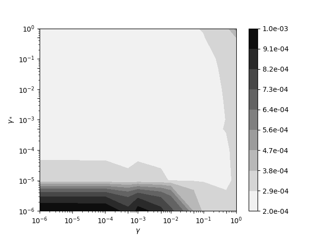
(a) $\mu=10^{-3}$.

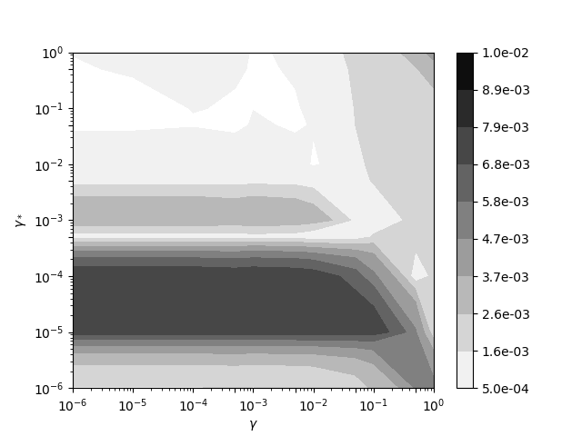
(b) $\mu=10^{-2}$.

Figure 5. Varying the stabilization parameters $\gamma$ and $\gamma_{*}$. Absolute $L^{2}$-errors downstream, computational domains in Figure 4(a). $\beta=(1,0)$, exact solution $u=2\sin(5\pi x)\sin(5\pi y)$. Similar results in the upstream case.

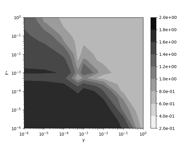
(a) $\mu=10^{-3}$.

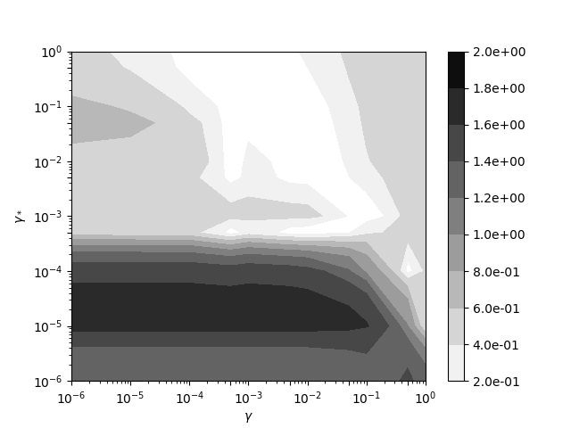
(b) $\mu=10^{-2}$.

Figure 6. Varying the stabilization parameters $\gamma$ and $\gamma_{*}$. Absolute $L^{2}$-errors globally, computational domains in Figure 4(a). $\beta=(1,0)$, exact solution $u=2\sin(5\pi x)\sin(5\pi y)$.

We first show convergence plots both downstream and upstream from the data set when varying the diffusion coefficient $\mu$ and keeping the convection field $\beta$ fixed. As in the case of well-posed convection-dominated problems, the observed $L^{2}$-convergence order is typically $\mathcal{O}(h^{2})$, surpassing by $\mathcal{O}(h^{\frac{1}{2}})$ the weighted error estimates proven for general meshes (see Figure 7, for example).

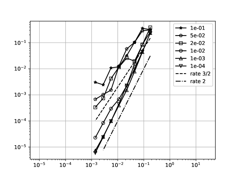
(a) Computational domains in Figure 4(b).

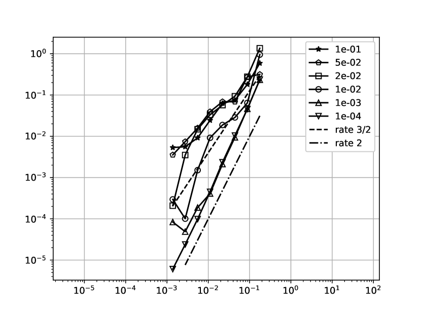
(b) Computational domains in Figure 4(c).

Figure 7. Absolute $L^{2}$-errors against mesh size $h$ when varying the diffusion coefficient $\mu$ for fixed $\beta=(1,0)$, exact solution $u=2\sin(5\pi x)\sin(5\pi y)$.

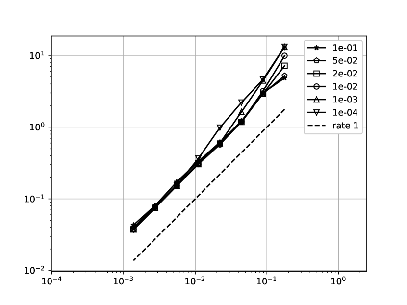
(a) Computational domains in Figure 4(b).

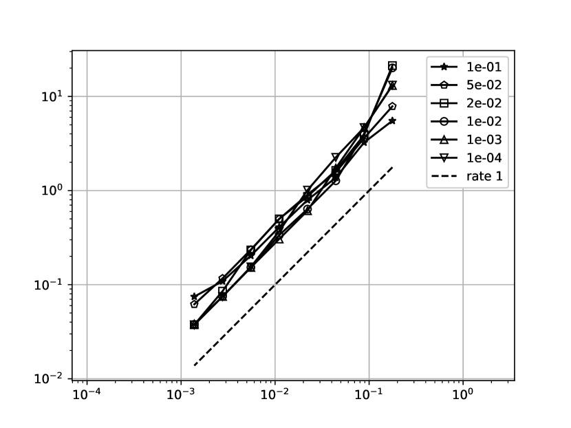
(b) Computational domains in Figure 4(c).

Figure 8. Absolute $H^{1}$-errors against mesh size $h$ when varying the diffusion coefficient $\mu$ for fixed $\beta=(1,0)$, exact solution $u=2\sin(5\pi x)\sin(5\pi y)$.

5.1. Data set near the inflow/outflow boundary

We consider the data set $\omega$ near the inflow and outflow boundaries of $\Omega$, as assumed in Section 2.1. We observe in Figure 7 that as diffusion is reduced the convergence order for the $L^{2}$-errors increases, culminating with quadratic convergence when convection dominates. Confirming the theoretical analysis in Section 4.4, we note the presence of an intermediate regime for Péclet numbers in which the upstream convergence orders are reduced and the upstream errors are typically larger. This can also be seen in Figure 9 where we consider the diffusion coefficient $\mu=10^{-2}$ and an interior data set. The errors in the $H^{1}$-seminorm are given in Figure 8 which shows almost linear convergence. This is probably due to the small contribution of the gradient term in the triple norm (23).

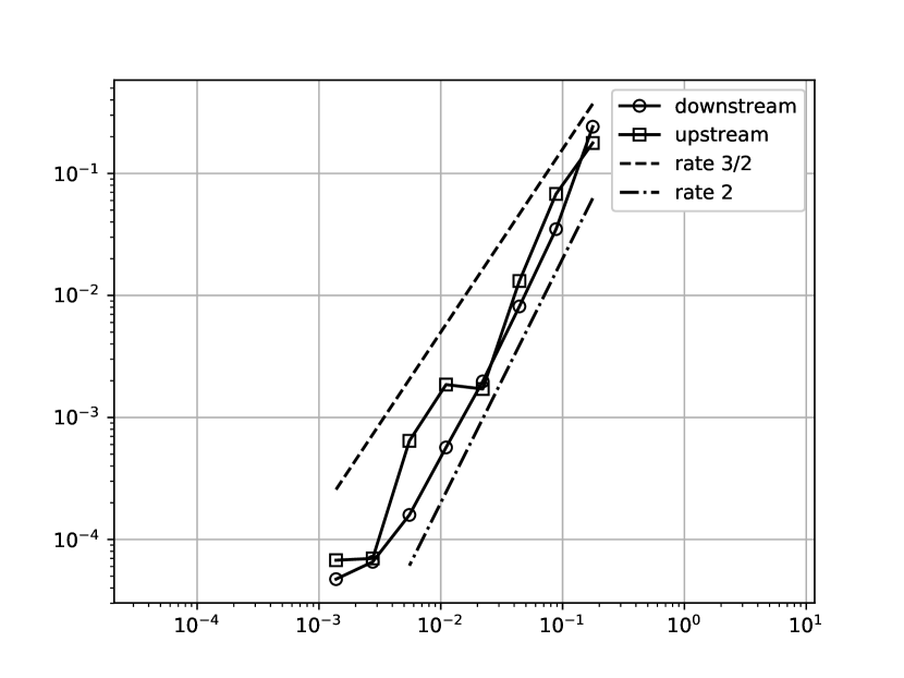
(a) Domains in Figure 4(a).

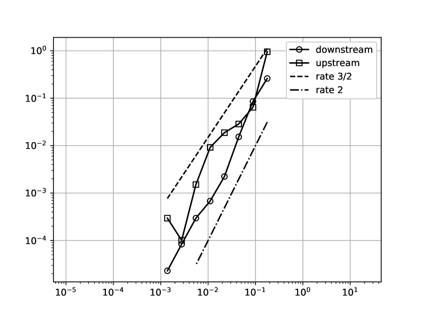
(b) Domains in Figure 4(b) and Figure 4(c).

Figure 9. Absolute $L^{2}$-errors against mesh size $h$, downstream vs upstream for $\mu=10^{-2}$, $\beta=(1,0)$, exact solution $u=2\sin(5\pi x)\sin(5\pi y)$.

(a) Downstream.

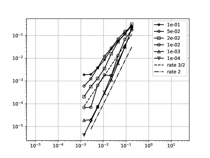
(b) Upstream.

Figure 10. Absolute $L^{2}$-errors against mesh size $h$, computational domains in Figure 4(a). Varying the diffusion coefficient $\mu$ for fixed $\beta=(1,0)$, exact solution $u=2\sin(5\pi x)\sin(5\pi y)$.

5.2. Interior data set

Next we consider the setting of the example discussed in the Introduction (Figure 2), where data is given in the centre of the domain. We give the convergence of the $L^{2}$-errors in Figure 10 with the caveat that this location of the data set $\omega$ is not rigorously covered by the theoretical analysis of the previous sections. Nonetheless, the experiments are in agreement with the proven results. Notice that the $L^{2}$-convergence is faster as $\mu$ decreases and for high Péclet numbers (above 10) one has optimal quadratic convergence both downstream and upstream, with the distinction that in the upstream case the convergence order is reduced in an intermediate regime, in agreement with the theoretical results in Section 4. Also, as expected from the error estimates proven in the first part [BNO20], when diffusion is moderately small one can see the transition towards the diffusion-dominated regime as the mesh gets refined – the convergence changes from almost quadratic to sublinear as the Péclet number decreases below 1. Figure 11 shows almost linear convergence in the $H^{1}$-seminorm. We think this is observed due to the small contribution of the gradient term in the triple norm (23). We also remark almost no distinction between upstream and downstream for this example, probably because the gradient term is controlled by the $L^{2}$-norm for small enough $\mu$.

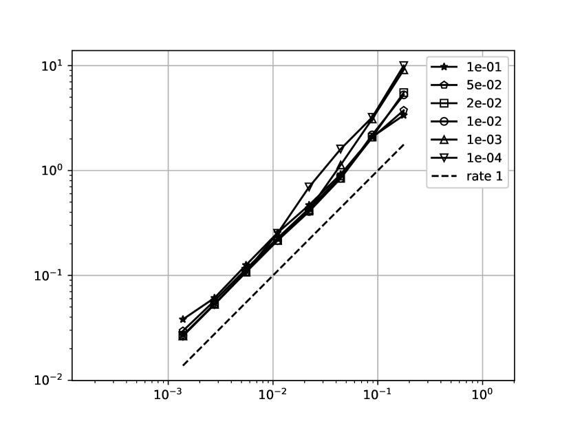
(a) Downstream.

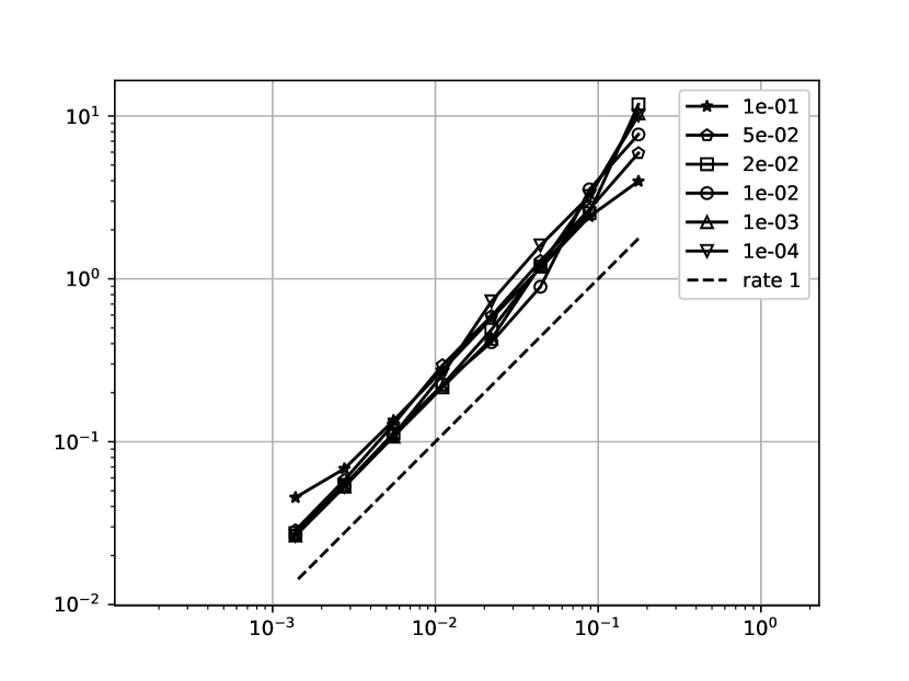
(b) Upstream.

Figure 11. $H^{1}$-errors against mesh size $h$, computational domains in Figure 4(a). Varying the diffusion coefficient $\mu$ for fixed $\beta=(1,0)$, exact solution $u=2\sin(5\pi x)\sin(5\pi y)$.

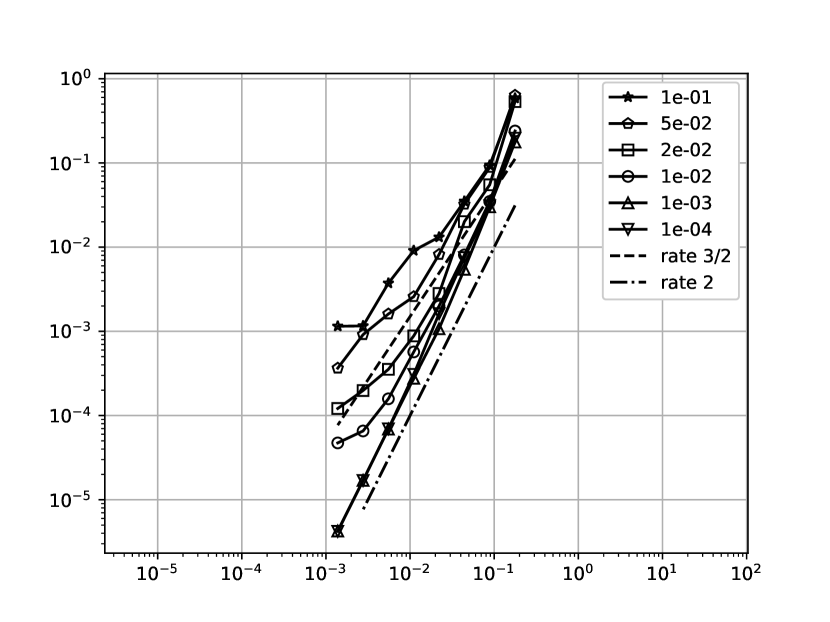
(a) Downstream, perturbation $\mathcal{O}(h^{2})$.

(b) Upstream, perturbation $\mathcal{O}(h^{2})$.

Figure 12. $L^{2}$-errors against mesh size $h$ for perturbations in data, computational domains in Figure 4(a). Varying the diffusion coefficient $\mu$ for fixed $\beta=(1,0)$, exact solution $u=2\sin(5\pi x)\sin(5\pi y)$.

5.3. Data perturbations

We demonstrate the effect of data perturbations $\tilde{U}_{\omega}=u|_{\omega}+\delta$ in a downstream vs upstream setting by polluting the restriction of $u$ to each node of the mesh in $\omega$ with uniformly distributed values in $[-h^{2},h^{2}],[-h,h]$ and $[-h^{\frac{1}{2}},h^{\frac{1}{2}}]$, respectively. Comparing first Figure 12 to Figure 10 we see that perturbations of amplitude $\mathcal{O}(h^{2})$ have no effect on the $L^{2}$-errors, as expected.

An $\mathcal{O}(h)$ noise amplitude exhibits in Figure 13 the difference – proven in Theorem 1 and Theorem 2 – between the downstream and upstream scenarios. In the upstream case the noise has a strong effect for moderate Péclet numbers and the errors stagnate. Only for high Péclet numbers one has convergence of order $\mathcal{O}(h^{\frac{1}{2}})$. In the downstream case one observes lower errors, faster convergence and almost no noise effect for high Péclet numbers. The difference is also very clear for perturbations of amplitude $\mathcal{O}(h^{\frac{1}{2}})$ shown in Figure 14. In the upstream case the errors stagnate and there seems to be no convergence, while in the downstream case the errors still convergence for high Péclet numbers.

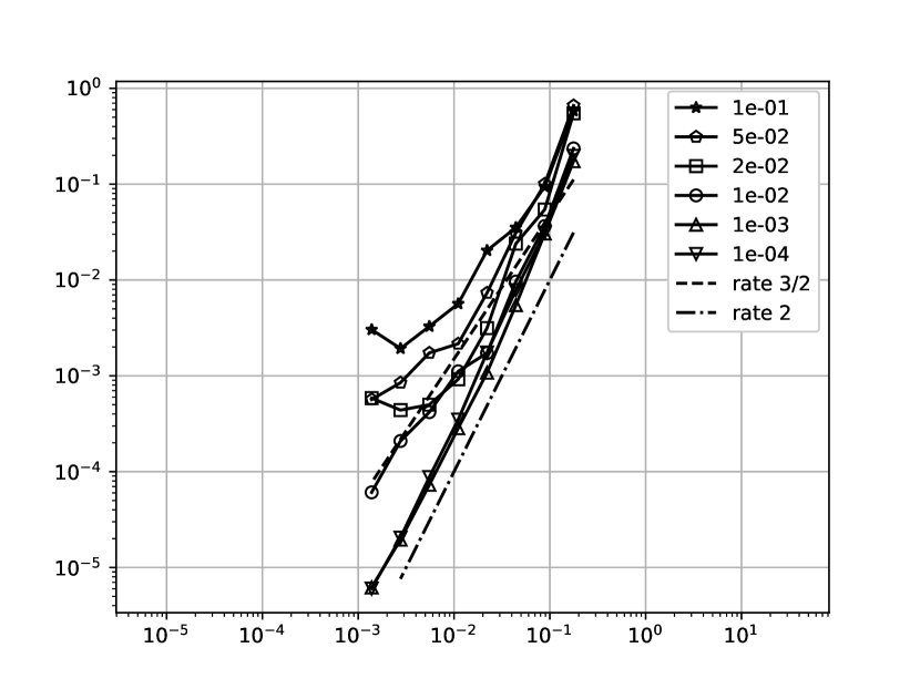
(a) Downstream, perturbation $\mathcal{O}(h)$.

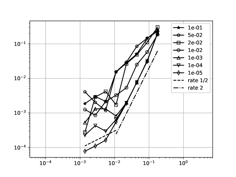
(b) Upstream, perturbation $\mathcal{O}(h)$.

Figure 13. $L^{2}$-errors against mesh size $h$ for perturbations in data, computational domains in Figure 4(a). Varying the diffusion coefficient $\mu$ for fixed $\beta=(1,0)$, exact solution $u=2\sin(5\pi x)\sin(5\pi y)$.

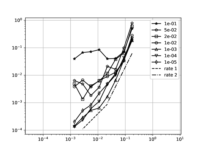
(a) Downstream, perturbation $\mathcal{O}(h^{\frac{1}{2}})$.

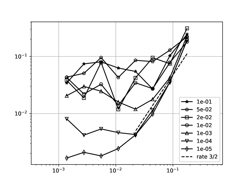
(b) Upstream, perturbation $\mathcal{O}(h^{\frac{1}{2}})$.

Figure 14. $L^{2}$-errors against mesh size $h$ for perturbations in data, computational domains in Figure 4(a). Varying the diffusion coefficient $\mu$ for fixed $\beta=(1,0)$, exact solution $u=2\sin(5\pi x)\sin(5\pi y)$.

5.4. Internal layer example

We now consider an exact solution $u=\sin(3\pi x)+\tanh(100(y-1/2))$ having an internal layer at $y=1/2$ and study qualitatively the transition from dominant diffusion to dominant convection. Data is given on both sides of the layer. The distribution of the absolute error is presented in Figure 15 for the diffusion-dominated regime and in Figure 16 for the intermediate and convection-dominated regimes. Note that the width of the internal layer does not depend on the physical parameters. Initially, the errors oscillate away from the data sets and concentrate around the boundary of the domain. When convection dominates, the approximation around the layer strongly deteriorates due to the crosswind position relative to the data sets. In this example the mesh is unstructured with 512 elements on a side and $h\approx 0.0025$.

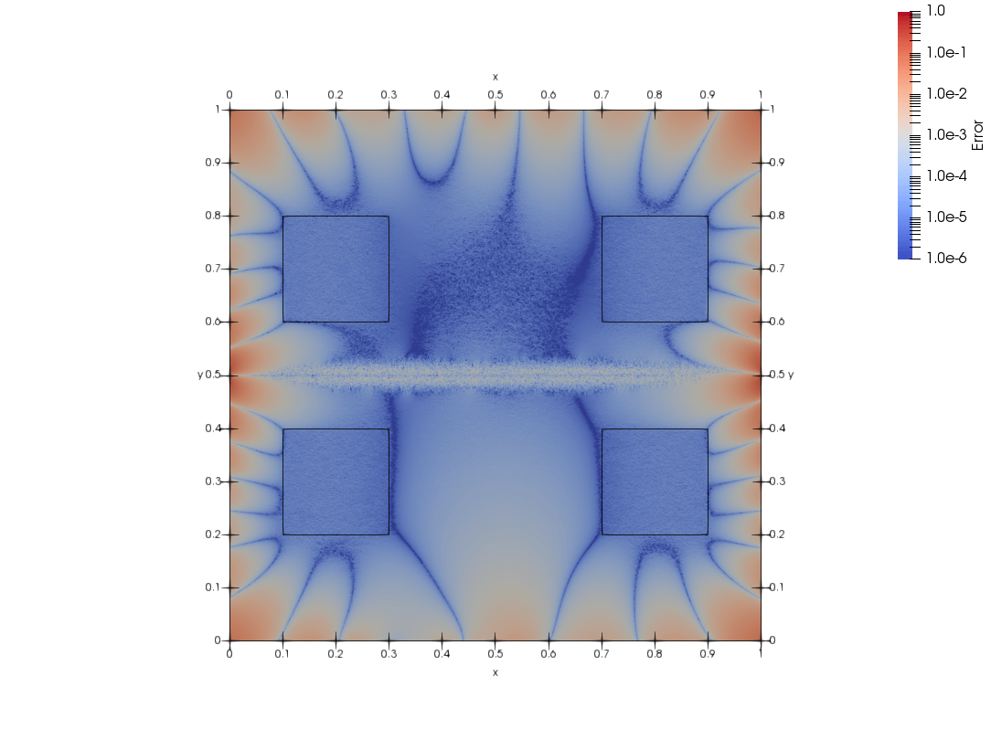
Figure 15. Absolute error in the diffusion-dominated regime, $\mu=1,\,\beta=(1,0)$. Data given in the four outlined boxes for the solution $u=\sin(3\pi x)+\tanh(100(y-1/2))$.

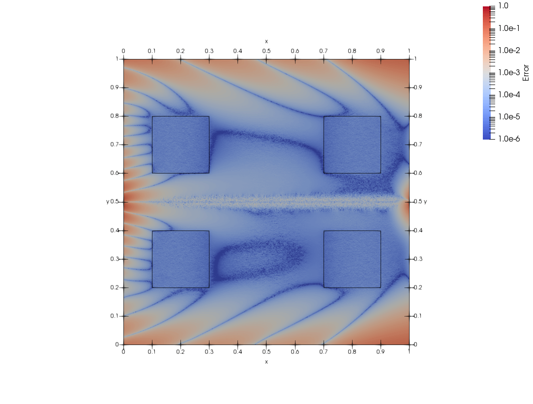
(a) $\mu=10^{-2}.$

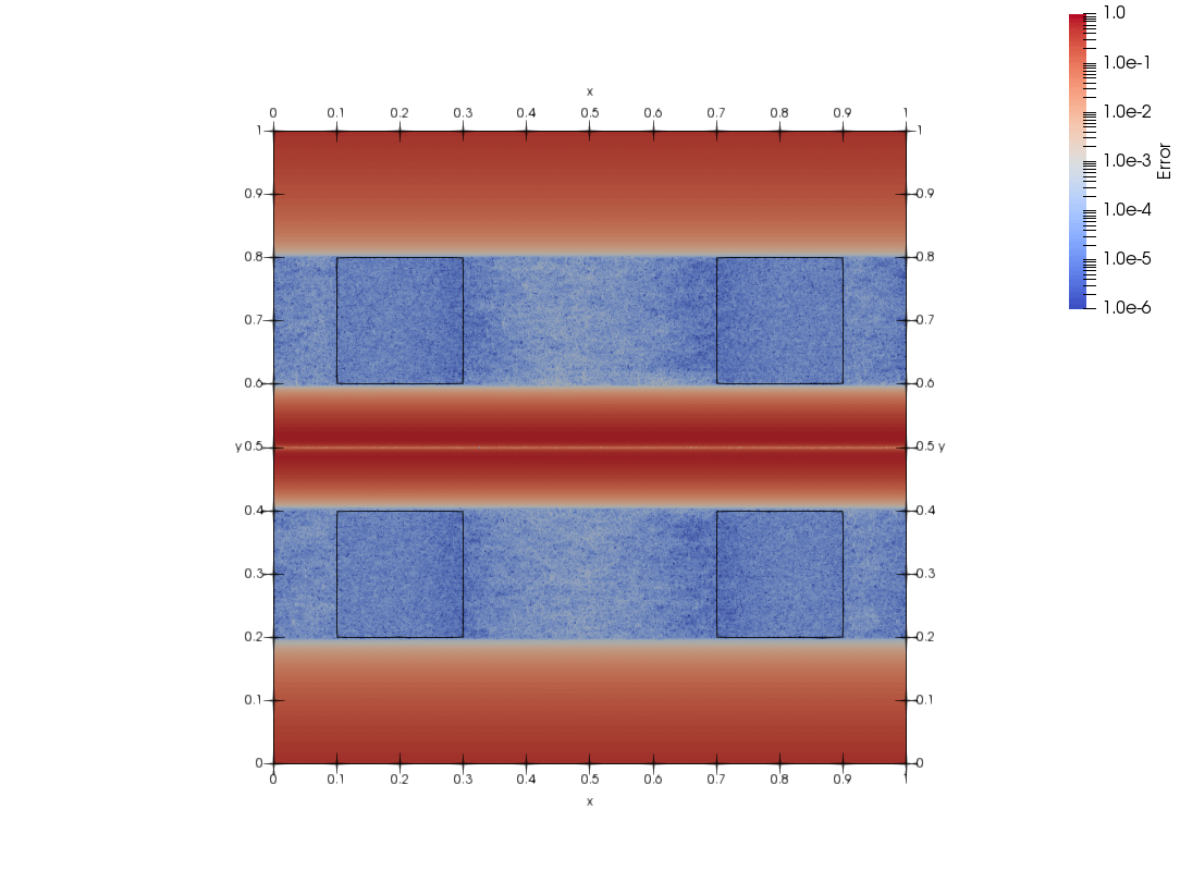
(b) $\mu=10^{-6}.$

Figure 16. Absolute error in transition to the convection-dominated regime, $\beta=(1,0)$. Data given in the four outlined boxes for the solution $u=\sin(3\pi x)+\tanh(100(y-1/2))$.

References

• [ABH+15] M. S. Alnæs, J. Blechta, J. Hake, A. Johansson, B. Kehlet, A. Logg, C. Richardson, J. Ring, M. E. Rognes, and G. N. Wells. The FEniCS Project Version 1.5. Archive of Numerical Software, 3(100):9–23, 2015.
• [Ber99] S. Bertoluzza. The discrete commutator property of approximation spaces. C. R. Acad. Sci. Paris Sér. I Math., 329(12):1097–1102, 1999.
• [BGL09] E. Burman, J. Guzmán, and D. Leykekhman. Weighted error estimates of the continuous interior penalty method for singularly perturbed problems. IMA J. Numer. Anal., 29(2):284–314, 2009.
• [BHL18] E. Burman, P. Hansbo, and M. G. Larson. Solving ill-posed control problems by stabilized finite element methods: an alternative to Tikhonov regularization. Inverse Problems, 34:035004, 2018.
• [BNO20] E. Burman, M. Nechita, and L. Oksanen. A stabilized finite element method for inverse problems subject to the convection–diffusion equation. I: diffusion-dominated regime. Numer. Math., 144(451–477), 2020.
• [Bur05] E. Burman. A unified analysis for conforming and nonconforming stabilized finite element methods using interior penalty. SIAM J. Numer. Anal., 43(5):2012–2033, 2005.
• [Bur13] E. Burman. Stabilized finite element methods for nonsymmetric, noncoercive, and ill-posed problems. Part I: Elliptic equations. SIAM J. Sci. Comput., 35(6):A2752–A2780, 2013.
• [Bur14] E. Burman. Stabilized finite element methods for nonsymmetric, noncoercive, and ill-posed problems. Part II: Hyperbolic equations. SIAM J. Sci. Comput., 36(4):A1911–A1936, 2014.
• [BV07] R. Becker and B. Vexler. Optimal control of the convection-diffusion equation using stabilized finite element methods. Numer. Math., 106(3):349–367, 2007.
• [DQ05] L. Dede’ and A. Quarteroni. Optimal control and numerical adaptivity for advection-diffusion equations. M2AN Math. Model. Numer. Anal., 39(5):1019–1040, 2005.
• [EG04] A. Ern and J.-L. Guermond. Theory and practice of finite elements, volume 159 of Applied Mathematical Sciences. Springer-Verlag, New York, 2004.
• [Eva10] L. C. Evans. Partial differential equations, volume 19 of Graduate Studies in Mathematics. American Mathematical Society, 2010.
• [HYZ09] M. Hinze, N. Yan, and Z. Zhou. Variational discretization for optimal control governed by convection dominated diffusion equations. J. Comput. Math., 27(2-3):237–253, 2009.
• [JKN18] V. John, P. Knobloch, and J. Novo. Finite elements for scalar convection-dominated equations and incompressible flow problems: a never ending story? Comput. Vis. Sci., 19(5):47–63, Dec 2018.
• [JNP84] C. Johnson, U. Nävert, and J. Pitkäranta. Finite element methods for linear hyperbolic problems. Comput. Methods Appl. Mech. Engrg., 45(1-3):285–312, 1984.
• [MS99] P. Monk and E. Süli. The adaptive computation of far-field patterns by a posteriori error estimation of linear functionals. SIAM J. Numer. Anal., 36(1):251–274, 1999.
• [NS74] J. A. Nitsche and A. H. Schatz. Interior estimates for Ritz-Galerkin methods. Math. Comp., 28(128):937–958, 1974.
• [RS15] H.-G. Roos and M. Stynes. Some open questions in the numerical analysis of singularly perturbed differential equations. Comput. Methods Appl. Math., 15(4):531–550, 2015.
• [Ste70] E. M. Stein. Singular integrals and differentiability properties of functions, volume 30 of Princeton Mathematical Series. Princeton University Press, 1970.
• [YZ09] N. Yan and Z. Zhou. A priori and a posteriori error analysis of edge stabilization Galerkin method for the optimal control problem governed by convection-dominated diffusion equation. J. Comput. Appl. Math., 223(1):198–217, 2009.