Analytical Survival Analysis of the Ornstein-Uhlenbeck Process

Abstract

We use asymptotic methods from the theory of differential equations to obtain an analytical expression for the survival probability of an Ornstein-Uhlenbeck process with a potential defined over a broad domain. We form a uniformly continuous analytical solution covering the entire domain by asymptotically matching approximate solutions in an interior region, centered around the origin, to those in boundary layers, near the lateral boundaries of the domain. The analytic solution agrees extremely well with the numerical solution and takes into account the non-negligible leakage of probability that occurs at short times when the stochastic process begins close to one of the boundaries. Given the range of applications of Ornstein-Uhlenbeck processes, the analytic solution is of broad relevance across many fields of natural and engineering science.

1 Introduction

The generalized Ornstein-Uhlenbeck (OU) model describes a stochastic process with at least one equilibrium point. It provides a framework for a wide range of physical, biological and social systems, wherein stabilization is viewed in terms of a potential minimum, characterized by a negative Lyapunov exponent, and high-frequency fluctuations are interpreted in terms of specific noise forcing. For example, an OU process is used to study neuronal activity Ricciardi1979 and the time-evolution of trait values towards their evolutionary optima OMeara2014 . In a clinical setting the health of the hepatic dynamic equilibrium is fit to an OU process using maximum likelihood estimation. Stochastic volatility, crucial for deducing stock returns or option pricing, is treated in terms of an OU process Schobel1999 , as are the noise spectra of climate observations Hasselmann1976 ; Moon2017 ; MAW2018 .

A particular stochastic model is commonly studied in terms of the survival probability, which is associated with the probability of one or more events occurring, or for the system to reach a defined threshold for the first time starting from a given initial position. Due to the generality of the question it addresses, survival analysis has been widely used in science and engineering. Examples include Feshbach resonances and the quantum Zeno effect (for example Feshbach ; Zeno1 ; Zeno2 ), engineering reliability analysis Zacks2012 , financial risk management McNeil2015 , and event history analysis in sociology Blossfeld2014 . Moreover, in the specific case of an OU process survival analyses from neuroscience Tuckwell1988 and epidemiology Mode2000 ; Madec2004 to quantitative finance Leblanc1998 ; Linetsky2004 ; Jeanblanc2000 and extreme value statistics of correlated random variables Majumdar2020 demonstrate the ubiquity of the approach. Our survival analysis is broadly relevant to all systems that can be described by an OU process. For example, it can be shown Gautie2019 that the survival probability of Brownian motion with an absorbing boundary that moves in time $t$ as $\propto\sqrt{t}$ can be recast as an OU process with a fixed absorbing boundary using Lamperti’s (or Doob’s) transformation.

Let $\{X(t),\,t\geq 0\}$ be an OU process starting at $x$. The time it takes for the state of a system to encounter a threshold ${\color[rgb]{0,0,0}X(t)=\beta}$ for the first time is variously called the first hitting time or first passage time, whose probability distribution function ${\color[rgb]{0,0,0}\zeta(t,x)}$, is defined as

$${\color[rgb]{0,0,0}\zeta(t,x)=\frac{\partial}{\partial t}\textrm{Prob}\{T\leq t\}},$$ (1)

where

$${\color[rgb]{0,0,0}T\equiv\textrm{inf}\{t\,:\,X(t)>\beta|X(0)=x\}.}$$ (2)

The time integral of the probability distribution of the first passage time is the survival probability (see for example Bray2013 ; Redner2001 ; Alili2005 ; Rich for reviews).

Despite the broad applicability of the survival probability, a simple accurate analytical expression has been lacking, which is the primary motivation of our work. The exact mathematical form is constructed using the Laplace transform and its inverse, which results in a series expansion of special functions Darling1953 . However, its complexity confounds practical implementation. In particular, when the initial data are close to the boundary of the confining potential Dolgoarshinnykh2006 , or when the boundary itself is near the equilibrium point Ditlevsen2005 , one must retain a considerable number of terms in the expansion.

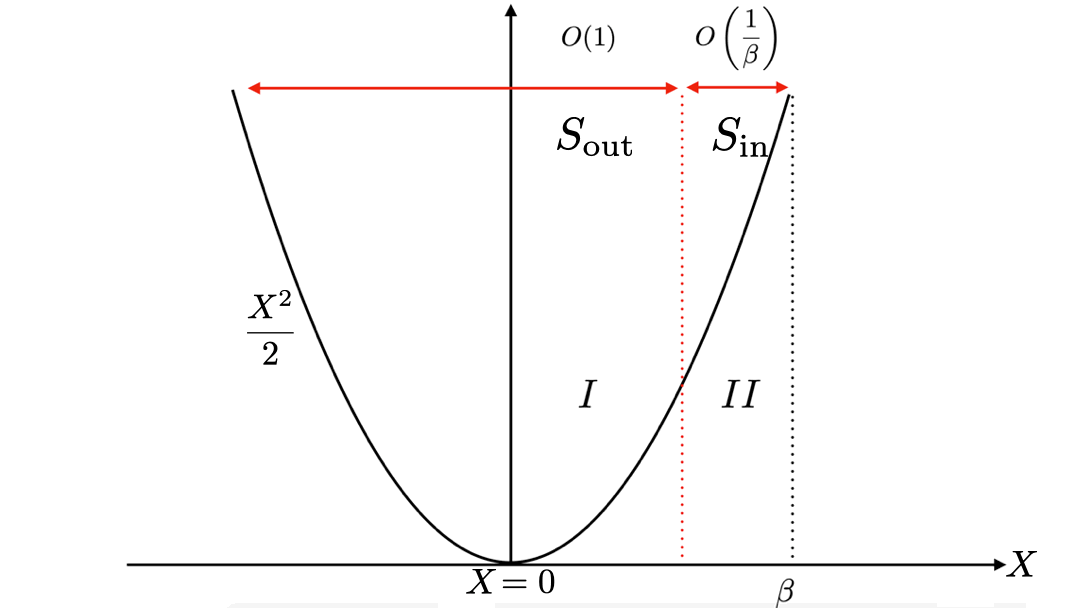
Figure 1: Schematic of the problem under study; what is the probability that a particle reaches the edge of the potential well? We divide the potential into an “outer” region $I$ and a boundary layer $II$, or the “inner” region, of the potential, in each of which the asymptotically dominant solutions are determined and then matched.

Our treatment of survival probability is shown in the schematic potential of Fig. 1, which contains a particle governed by a one-dimensional Ornstein-Uhlenbeck process through an overdamped autonomous Langevin equation given by

$${\color[rgb]{0,0,0}\dot{X}(t)=-aX(t)+\sqrt{2b}\xi(t)},$$ (3)

where $a$ and $b$ are positive constants and $\xi(t)$ is Gaussian white noise with a zero mean and $\langle\xi(t)\xi(s)\rangle=\delta(t-s)$.

The survival probability commonly characterizes the anomalous or abnormal behavior of a system. This motivates our consideration of a threshold state (${\color[rgb]{0,0,0}X=\beta}$) far from the equilibrium state (${\color[rgb]{0,0,0}X(t)=0}$), so that it is rare that the system will reach the threshold.

The next section is devoted to our overall approach. In §2.1 we summarize our method. In §2.2 we briefly review previous results on the survival probability of an OU process that will be used in §2.3 to derive a simple analytical expression that reproduces the survival probability for large values of the domain boundaries and when the initial data are close to the boundary. In §2.4 we compare the analytical and numerical results.

2 Using Matched Asymptotic Methods to Determine the Survival Probability

2.1 Summary of Analytical Method

Our approach is as follows. As shown in Fig. 1 we divide the domain into two regions footnote : a broad $O(1)$ region ($I$) containing the minimum of the potential, ${\color[rgb]{0,0,0}X=0}$, and a narrow $O\left({1}/{\beta}\right)$ boundary layer near ${\color[rgb]{0,0,0}X=\beta}$. We solve the limiting differential equations in these regions, from which we develop a uniform composite solution for the probability density of the survival probability using asymptotic matching, which is a highly accurate general analytical method Bender2013 , recently used to obtain the solution to the related problem of stochastic resonance Moon2020 .

2.2 Previous Results on the Survival Probability of an OU Process

The canonical approach of finding the survival probability of this OU process is to determine the probability distribution for the first hitting time in Laplace space

$${\color[rgb]{0,0,0}\tilde{\zeta}(\lambda,x)=\int_{0}^{\infty}e^{-\lambda t}\zeta(t,x)dt,}$$ (4)

which leads to the following analytical expression Siegert1951 ; Srinivasan2013 ; Ricciardi2013 ,

$$\tilde{\zeta}(\lambda,x)=\,e^{\frac{a(x^{2}-\beta^{2})}{4b}}\frac{D_{-\lambda/a}(-x\sqrt{a/b})}{D_{-\lambda/a}(-\beta\sqrt{a/b})},$$ (5)

where $D_{\lambda}(z)$ is the parabolic cylinder function, $\beta$ is the boundary position and $x$ is the initial position.

This equation can be written as a spectral decomposition Ricciardi1988 , wherein the countable number of eigenvalues correspond to the zeros of the denominator of Eq. (5). The final expression for the probability distribution of the first hitting time can be obtained by inverting each term of this spectral decomposition, which can be written as a weighted sum of exponential functions as

$$\begin{split}\zeta(t,x)=\sum_{p=0}^{\infty}e^{\lambda_{p}(\beta)t}\frac{\Phi(\lambda_{p}(\beta)/a,x\sqrt{a/b})}{\Phi^{\prime}(\lambda_{p}(\beta)/a,\beta\sqrt{a/b})},\end{split}$$ (6)

where $\lambda_{p}(\beta)$ is the solution of

$$\Phi(\lambda_{p}(\beta)/a,\beta\sqrt{a/b})=0,$$ (7)

and $\Phi$ and $\Phi^{\prime}$ are defined in Ricciardi1988 in terms of Kummer and digamma functions.

For large values of $t$ and $\beta-x$, Eq. (6) simplifies considerably. In fact, because all the eigenvalues, $\lambda_{p}(\beta)$, are negative, only that with the smallest magnitude will contribute significantly as $t\to\infty$. Moreover, for large values of $\beta-x$, Eq. (6) becomes

$$\begin{split}\lim_{\beta-x\to\infty}\zeta(t,x)&=\frac{1}{t_{1}(\beta;0)}\exp\left[-\frac{t}{t_{1}(\beta;0)}\right]\qquad\textrm{with}\\ t_{1}(\beta;0)&=\frac{1}{a\beta}\sqrt{\frac{2\pi b}{a}}\exp\left[\frac{a\beta^{2}}{2b}\right],\end{split}$$ (8)

where $t_{1}(\beta;0)$ is the mean first passage time of the process from $X(t=0)=0$ to the boundary $\beta$ Nobile1985 .

Importantly, however, the asymptotic expression in Eq. (8) is not valid when $x\approx\beta$. Indeed, as we show here, when the process starts in the neighborhood of $x=\beta$ there is a non-trivial leakage of probability. This leakage is not taken into account by Eq. (8) and transpires very rapidly, on a time scale of order $1/\beta^{2}$. Therefore, taking this approach requires that one calculate an enormous number of eigenvalues in Eq. (6), which is computationally inefficient. Our approach avoids this problem.

2.3 Detailed Development of the Approach

We derive an asymptotic expression for the survival probability, which is the time integral of the probability distribution of the first passage time, in the large $\beta$ limit that is trivial to evaluate when $x\approx\beta$.

The probability density, $\rho(y,t;x,s)$, of the OU process in Eq. (3) is described by the Kolmogorov forward (KFE) and backward (KBE) equations, the former of which is

$$\partial_{t}\rho(y,t;x,s) =a~{}\partial_{y}[y(t)\rho(y,t;x,s)]$$ (9)

$$+b~{}\partial_{yy}\rho(y,t;x,s)\,\equiv\mathcal{L}_{y}\rho(y,t;x,s),$$

where the operator $\mathcal{L}_{y}$ is the generator of the OU process viz., $[\mathcal{L}_{y}f](y,t)=a~{}\partial_{y}[yf(y,t)]+b~{}\partial_{yy}f(y,t)$. The KBE follows by replacing $\mathcal{L}_{y}$ with its adjoint, $\mathcal{L}_{x}^{*}$, defined as $[\mathcal{L}_{x}^{*}f](x,s)=-ax~{}\partial_{x}f(x,s)+b~{}\partial_{xx}f(x,s)$.

The KFE gives the evolution of the probability density of the process when the initial position and time, ($x,s$), are known, while the KBE treats the evolution when the final position and time, ($y,t$), are known. Both equations have initial condition

$$\rho(y,u;x,u)=\delta(y-x),$$ (10)

and boundary conditions

$$\rho(\pm\infty,t;x,s)=0\qquad\textrm{and}\qquad\rho(y,t;\pm\infty,s)=0$$ (11)

for the KFE and the KBE respectively.

The survival probability within the interval $(\alpha,\beta)$ is defined in terms of the KBE density, $\rho_{KBE}$, as

$$S(t;x,s)=\int_{\alpha}^{\beta}\rho_{KBE}(y,t;x,s)dy,$$ (12)

which satisfies

$$\begin{split}-\partial_{s}S(t;x,s)=-a~{}x(s)\partial_{x}S(t;x,s)+b~{}\partial_{xx}S(t;x,s),\end{split}$$ (13)

with initial condition

$$S(t=s;x,s)=\Theta(x-\alpha)\Theta(\beta-x),$$ (14)

and boundary conditions

$$S(t;x=\alpha,s)=S(t;x=\beta,s)=0\;\;\;\forall\;s\leq t,$$ (15)

where $\Theta(\cdot)$ is the Heaviside theta function.

Let $P_{i}^{\alpha}(P_{i}^{\beta})$ be the probability of hitting $x=\alpha(\beta)$ for the first time after $i$ time steps and let $S^{\alpha}(S^{\beta})$ be the survival probability with an absorbing boundary at $x=\alpha(\beta)$. Hence, if we discretize the stochastic process, the survival probability after $n$ time steps is

$$\begin{split}S_{n}&=\prod_{i=1}^{n}(1-P_{i}^{\alpha}-P_{i}^{\beta})=\prod_{i=1}^{n}[(1-P_{i}^{\alpha})(1-P_{i}^{\beta})-P_{i}^{\alpha}P_{i}^{\beta}]\\ &\simeq\prod_{i=1}^{n}(1-P_{i}^{\alpha})\prod_{i=1}^{n}(1-P_{i}^{\beta})=S_{n}^{\alpha}S_{n}^{\beta}.\end{split}$$ (16)

In the second line of Eq. (16), we have neglected the term $P_{i}^{\alpha}P_{i}^{\beta}$ when $|\alpha|\gg 1$ and $|\beta|\gg 1$, allowing us to write the survival probability in the interval $(\alpha,\beta)$ as the product of the two survival probabilities in the two intervals $(-\infty,\beta)$ and $(\alpha,\infty)$ with $\alpha<\beta$. From this point we will only consider the survival probability in the interval $(-\infty,\beta)$, and note that the derivation for the interval $(\alpha,\infty)$ is in straightforward analogy.

We now rewrite Eq. (13) in a rescaled form,

$$\begin{split}\partial_{t}S(x,t)=-x(t)\partial_{x}S(x,t)+\partial_{xx}S(x,t),\end{split}$$ (17)

with the new variables,

$$x\to x\sigma,\;\;\;\beta\to\beta\sigma~{}~{}\textrm{and}~{}~{}s\to-\frac{t}{a},$$ (18)

in which the spatial coordinate is expressed in terms of the standard deviation $\sigma=\sqrt{b/a}$ of a stationary OU process obtained from the solution of Eq. (9) in the limit $t\to\infty$. The new initial and boundary conditions are

$$\begin{cases}S(x,t=0)=\Theta(\beta-x),\\ S(x=\beta,t)=0,\\ S(x=-\infty,t)=1.\end{cases}$$ (19)

We solve the limiting differential equations within the two regions, from which we construct an approximate uniform solution by asymptotic matching. We denote $S_{\textrm{out}}(x,t)$ and $S_{\textrm{in}}(x,t)$ the solutions in region $I$ and $II$ respectively.

Region $I$. The outer solution is obtained by imposing $\beta-x\gg 1$. In this limit the probability distribution of the first hitting time in Eq. (8) is valid, and its time integral gives the survival probability as

$$S_{\textrm{out}}(t){\simeq}\,\textrm{e}^{-\left(\frac{\beta}{\sqrt{2\pi}}\textrm{e}^{-\frac{\beta^{2}}{2}}\right)t},$$ (20)

where the rescaled $\beta$ and $t$ of Eq. (18) have been used.

Region $II$. In the boundary layer, or the inner region, we have $x\sim\beta$, where the approximation of Region $I$ is no longer valid. We let $\epsilon\equiv 1/\beta\ll 1$ and introduce the following stretched coordinates,

$$\eta=\frac{x-\frac{1}{\epsilon}}{\epsilon}~{}~{}\textrm{and}~{}~{}\theta=\frac{t}{\epsilon^{2}},$$ (21)

that we use to rewrite Eq. (17) as

$$\frac{1}{\epsilon^{2}}\partial_{\theta}S_{\textrm{in}}(\eta,\theta) =-\left[\frac{1}{\epsilon^{2}}+\eta(\theta)\right]\partial_{\eta}S_{\textrm{in}}(\eta,\theta)$$

$$+\frac{1}{\epsilon^{2}}\partial_{\eta\eta}S_{\textrm{in}}(\eta,\theta),$$ (22)

which at leading-order becomes

$$\partial_{\theta}S_{\textrm{in}}(\eta,\theta)=-\partial_{\eta}S_{\textrm{in}}(\eta,\theta)+\partial_{\eta\eta}S_{\textrm{in}}(\eta,\theta).$$ (23)

Clearly, Eq. (23) is a diffusion equation for $S_{\textrm{in}}(\eta,\theta)$ along the characteristics

$$\frac{d\eta}{d\theta}=1~{}~{}\textrm{and}~{}~{}\frac{d\rho}{d\theta}=1,$$ (24)

which we can then write as

$$\partial_{\rho}S_{\textrm{in}}(\mu,\rho)=\partial_{\mu\mu}S_{\textrm{in}}(\mu,\rho),$$ (25)

wherein $\mu\equiv\eta-\theta$ and $\rho\equiv\theta$, so that the boundary condition becomes $S_{\textrm{in}}(\mu=-\rho,\rho)=0$.

We solve Eq. (25) by first finding its Green’s function, $G(\rho,\mu;\nu)$, which satisfies

$$\partial_{\rho}G(\mu,\rho;\nu)-\partial_{\mu\mu}G(\mu,\rho;\nu)=\delta(\mu-\nu)\delta(\rho).$$ (26)

This Green’s function is associated with the probability density $\rho_{KBE}$, satisfying the KBE, and hence the survival probability through Eq. (12). Hence, this density satisfies the following conditions;

$$\begin{cases}\rho_{KBE}(\mu,\rho=0;\nu)=\delta(\mu-\nu),\\ \rho_{KBE}(\mu=0,\rho;\nu)=\rho_{KBE}(\mu=-\infty,\rho;\nu)=0.\end{cases}$$ (27)

The Green’s function is (e.g., Duffy2015 )

$$\begin{split}G(\rho,\mu;\nu)=&\frac{1}{\sqrt{4\pi\,\rho}}\bigg{(}\exp\left[-\frac{(\nu-\mu)^{2}}{4\,\rho}\right]-\\ &-\exp\left[-\frac{(\nu+\mu)^{2}}{4\,\rho}-\nu\right]\bigg{)},\end{split}$$ (28)

which, as noted above, now allows us to write the solution of Eq. (25) as

$$\begin{split}S_{\textrm{in}}(\mu,\rho)&=\int_{-\infty}^{0}d\nu\int_{-\infty}^{\infty}d\phi\,G(\mu,\rho;\phi)\delta(\phi-\nu)=\\ &=\int_{-\infty}^{0}d\nu\,G(\mu,\rho;\nu).\end{split}$$ (29)

Upon integration and reversion to the original variable $t$ and to the stretched coordinate $\eta$, we find

$$\begin{split}S_{\textrm{in}}(\eta,t){\simeq}&\frac{K}{2}\textrm{e}^{\eta}\bigg{(}-\textrm{erfc}\bigg{[}\frac{1}{2}\sqrt{\frac{1}{t}}(-t-\eta)\bigg{]}+\\ &+\textrm{e}^{-\eta}\textrm{erfc}\bigg{[}\frac{1}{2}\sqrt{\frac{1}{t}}(-t+\eta)\bigg{]}\bigg{)}{\color[rgb]{0,0,0}\equiv K\,S_{\textrm{in}}^{\prime}(\eta,t)}.\end{split}$$ (30)

We determine the constant $K$ by requiring the outer limit of the inner solution to equal the outer solution;

$$\begin{split}&K=\lim_{\eta\to-\infty}S_{\textrm{in}}(\eta,t)=S_{\textrm{out}}(t){\simeq}\textrm{e}^{-\left(\frac{\beta}{\sqrt{2\pi}}\textrm{e}^{-\frac{\beta^{2}}{2}}\right)t}.\end{split}$$ (31)

Therefore, the uniformly valid approximate composite analytical solution for the survival probability is

$$\begin{split}S(x,t)&=S_{\textrm{in}}(x,t)+S_{\textrm{out}}(t)-K\\ &{\simeq}\frac{1}{2}\textrm{e}^{-\left(\frac{\beta}{\sqrt{2\pi}}\textrm{e}^{-\frac{\beta^{2}}{2}}\right)t}\textrm{e}^{\beta(x-\beta)}\\ &\bigg{(}{\color[rgb]{0,0,0}-~{}}\textrm{erfc}\bigg{[}\frac{1}{2}\sqrt{\frac{1}{t}}(-t-\beta(x-\beta))\bigg{]}+\\ &+\textrm{e}^{-\beta(x-\beta)}\textrm{erfc}\bigg{[}\frac{1}{2}\sqrt{\frac{1}{t}}(-t+\beta(x-\beta))\bigg{]}\bigg{)}=\\ &\equiv S{\color[rgb]{0,0,0}^{\prime}}_{\textrm{in}}(x,t)S_{\textrm{out}}(t),\end{split}$$ (32)

written in terms of the original spatial coordinate $x$ rather that the stretched coordinate $\eta$.

2.4 Comparing Analytical and Numerical Results

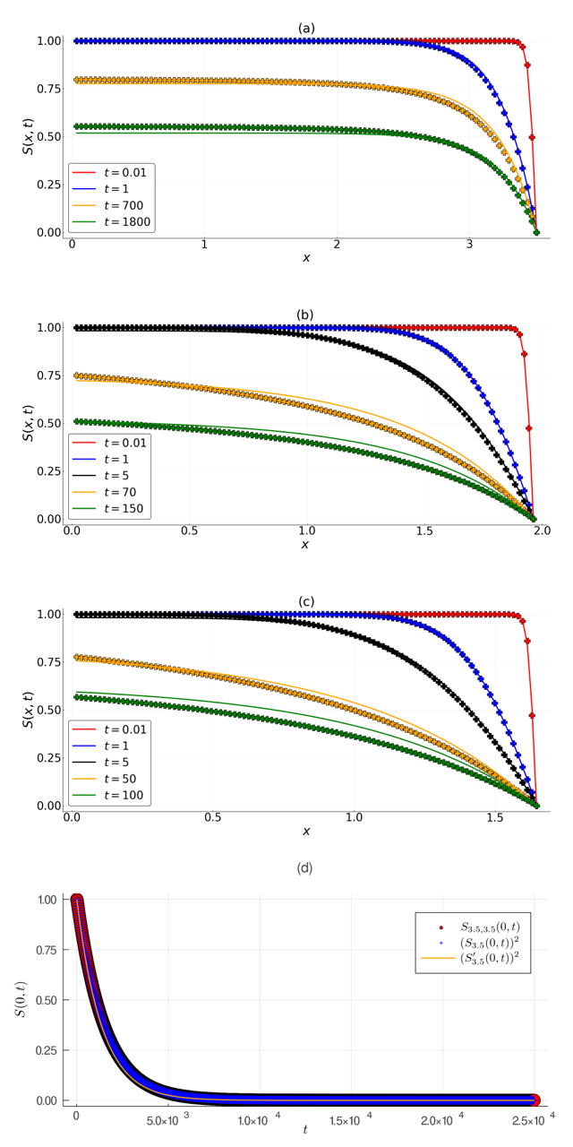
Figure 2: (a)-(c) Plot of Eq. (32), $S(x,t)$, versus $x\in[0,\beta]$ for different values of $t$ (solid lines) compared to the numerical solution of Eq. (17) (crosses). We use three different values of the boundary position $\beta$; (a) 3.5 (b) 1.96 and (c) 1.645, corresponding to the probability of finding the system below $x=\beta$ as $t\to\infty$ and without absorbing boundaries of (a) $99.95\%$, (b) $99\%$, and (c) $90\%$ respectively. (d) The numerical solution of Eq. (17) with two boundaries (red circles), $S_{\alpha,\beta}(x,t)$, $S_{\alpha}(x,t)S_{\beta}(x,t)$ (blue crosses), and the approximate analytical solution in Eq. (33)$,S^{\prime}_{\alpha}(x,t)S^{\prime}_{\beta}(x,t)$. Note that $S_{\alpha,\beta}(x,t)$ overlaps exactly with $S_{\alpha}(x,t)S_{\beta}(x,t)$. Here $\alpha=\beta=3.5$ and $x=0$.

We compare Eq. (32) with the numerical solution of Eq. (17) for different values of the parameter $\beta$ in Fig. (2), and find excellent agreement even when $\beta$ is not asymptotically large. Indeed, the smallest value of the distance to the boundary is $\beta=1.645\sigma$, corresponding to a $90\%$ probability that an unbounded stationary OU process remains below the boundary.

When $t\gg 1/\beta^{2}$ the left hand side of Eq. (23) is negligible and Eq. (32) becomes $S_{\textrm{out}}(t)[1-e^{\beta(x-\beta)}]$ and depends on time solely through $S_{\textrm{out}}(t)$, which is the prefactor of $S_{\textrm{in}}(x,t)$. Thus, depending on $x$ the rate of the decrease in the survival probability is controlled by $S_{\textrm{in}}(x,t)$, decaying more rapidly near the boundary for early times.

The accuracy of the asymptotic solutions over a wide range of the $\beta$ facilitates simple and wide ranging applications. For example, determining the input parameters of a leaky integrate-and-fire (LIF) neural model (see e.g., Lansky2008 and refs therein) based on experimentally observable interspike intervals Ditlevsen2005 . Of particular contemporary relevance is deducing the “critical community size” in disease epidemiology Dolgoarshinnykh2006 , or the population threshold below which infections do not persist.

Finally, we appeal to Eq. (16) to form the asymptotic expression for the survival probability of an Ornstein-Uhlenbeck process with two absorbing boundaries as

$$S_{\alpha,\beta}(x,t)=S{\color[rgb]{0,0,0}^{\prime}}^{\alpha}_{\textrm{in}}(x,t)S^{\alpha}_{\textrm{out}}(t)S{\color[rgb]{0,0,0}^{\prime}}^{\beta}_{\textrm{in}}(x,t)S^{\beta}_{\textrm{out}}(t)\;\forall t>s.$$ (33)

We note that only one of the boundary regions will contribute significantly viz.,

$$\begin{split}&S{\color[rgb]{0,0,0}^{\prime}}_{\textrm{in}}^{\alpha,\beta}(x,t)=S{\color[rgb]{0,0,0}^{\prime}}^{\alpha}_{\textrm{in}}(x,t)S{\color[rgb]{0,0,0}^{\prime}}^{\beta}_{\textrm{in}}(x,t)=S{\color[rgb]{0,0,0}^{\prime}}^{\gamma}_{\textrm{in}}(x,t),\\ &\gamma=\textrm{min}_{|h_{\alpha}|,|h_{\beta}|}(\alpha,\beta),\end{split}$$ (34)

where $h_{\alpha(\beta)}=x-\alpha(\beta)$.

In Fig. (2)(d) we show that the numerical solution with two boundaries matches that obtained by considering the two boundaries separately and with the analytical solution in Eq. (33).

3 Conclusion

We have obtained an asymptotic analytical solution for the survival probability of an Ornstein-Uhlenbeck process for large potentials. We divide the potential into two layers near the boundaries and a broad region between, which contains the origin, where we use the solution of Ricciardi & Sato Ricciardi1988 . The uniformly continuous solution is obtained by matching the two approximate solutions in the boundary layers with that in the broad region between. The solution agrees extremely well with both the numerical solution and with the more restricted asymptotic expression for the survival probability known in literature. Importantly, our analysis remains valid even when the initial position of the stochastic process is close to one of the boundaries, and furthermore it takes into account the non-negligible leakage of the probability early in the time evolution.

Despite the analysis using the assumption of asymptotically large boundaries, we showed that it agrees well with the numerical solution, even when the boundary positions are the same order of magnitude as the standard deviation of the stationary probability distribution function of the OU process. We demonstrate consistency even when there is a $90\%$ probability that the system without absorbing boundaries is found at a position less than $\beta$; when reaching the boundary can no longer be considered a rare event. Therefore, our method can be easily generalized to more general (less restrictive) settings. Finally, our compact analytical solution provides a computationally trivial framework for survival analysis of use across the broad spectrum of stochastic systems where the Ornstein-Uhlenbeck process arises.

References

- (1) L. M. Ricciardi and L. Sacerdote, The Ornstein-Uhlenbeck process as a model for neuronal activity, Biological Cybernetics, 35(1), 1-9 (1979).
- (2) B. C. O’Meara and J. M. Beaulieu, Modelling stabilizing selection: the attraction of Ornstein-Uhlenbeck models, in Modern Phylogenetic Comparative Methods and Their Application in Evolutionary Biology, p. 381-393 (Springer, Berlin, 2014).
- (3) D. C. Trost, E. A. Overman, J. H. Ostroff, W. Xiong and P. March, A model for liver homeostasis using modified mean-reverting Ornstein-Uhlenbeck process, Computational and Mathematical Methods in Medicine, 11(1), 27-47 (2010).
- (4) R. Schöbel and J. Zhu, Stochastic volatility with an Ornstein-Uhlenbeck process: an extension, Review of Finance, 3(1), 23-46 (1999).
- (5) K. Hasselmann, Stochastic climate models Part I. Theory, Tellus, 28(6), 473-485 (1976).
- (6) W. Moon and J. S. Wettlaufer, A unified nonlinear stochastic time series analysis for climate science, Sci. Rep., 7, 44228 (2017).
- (7) W. Moon, S. Agarwal and J. S. Wettlaufer, Intrinsic Pink-Noise Multidecadal Global Climate Dynamics Mode, Phys. Rev. Lett. 121, 108701 (2018).
- (8) F. V. Pepe, P. Facchi, Z. Kordi and S. Pascazio, Nonexponential decay of Feshbach molecules, Phys. Rev. A 101, 013632 (2020).
- (9) S. Maniscalco, J. Piilo, and K-A. Suominen, Zeno and Anti-Zeno Effects for Quantum Brownian Motion, Phys. Rev. Lett. 97, 130402 (2006).
- (10) F. Giacosa and G. Pagliara, Measurement of the neutron lifetime and inverse quantum Zeno effect, Phys. Rev. D 101, 056003 (2020).
- (11) S. Zacks, Introduction to Reliability Analysis: Probability Models and Statistical Methods (Springer, NY, 2012).
- (12) A. J. McNeil, R. Frey and P. Embrechts, Quantitative Risk Management: Concepts, Techniques and Tools-Eevised Edition (Princeton Univ. Press, Princeton, 2015).
- (13) H. Blossfeld, A. Hamerle and K. U. Mayer, Event History Analysis: Statistical Theory and Application in the Social Sciences (Psychology Press, NY, 2014).
- (14) H. C. Tuckwell, Introduction to Theoretical Neurobiology (volume 2): Nonlinear and Stochastic Theories (Cambridge University Press, Cambridge, 1988).
- (15) C. J. Mode and C. K. Sleeman, Stochastic Processes in Epidemiology: HIV/AIDS, Other Infectious Diseases, and Computers (World Scientific, Singapore, 2000).
- (16) Y. Madec and C. Japhet, First passage time problem for drifted Ornstein-Uhlenbeck process, Math. Biosci, 189, 131-140 (2004).
- (17) B. Leblanc and O. Scaillet, Path dependent options on yields in the affine term structure model, Finance and Stochastics, 2(4), 349-367 (1998).
- (18) V. Linetsky, Computing hitting time densities for CIR and OU diffusions: Applications to mean-reverting models, J. Comp. Finance, 7, 1-22 (2004).
- (19) M. Jeanblanc and M. Rutkowski, Modelling of default risk: An overview in Modern Mathematical Finance: Theory and Practice (Higher Ed. Press, Beijing, 2000).
- (20) S. N. Majumdar, A. Pal, G. Schehr, Extreme value statistics of correlated random variables: A pedagogical review, Phys. Rep. 840, 1 (2020).
- (21) T. Gautié, P. Le Doussal, S. N. Majumdar & G. Schehr, Non-crossing Brownian paths and Dyson Brownian motion under a moving boundary, J. Stat. Phys. 177(5), 752-805 (2019).
- (22) A. J. Bray, S. N. Majumdar and G. Schehr, Persistence and first-passage properties in nonequilibrium systems, Adv. Phys. 62, 225-361 (2013).
- (23) S. Redner, A Guide to First-Passage Processes (Cambridge University Press, Cambridge, 2001).
- (24) L. Alili, P. Patie and J. L. Pedersen, Representations of the first hitting time density of an Ornstein-Uhlenbeck process, Stochastic Models, 21(4), 967-980 (2005).
- (25) R. J. Martin , M. J. Kearney and R. V. Craster, Long- and short-time asymptotics of the first-passage time of the Ornstein-Uhlenbeck and other mean-reverting processes, J. Phys. A: Math. Theor. 52 134001 (2019).
- (26) D. A. Darling and A. J. F. Siegert, The First Passage Problem for a Continuous Markov Process, Ann. Math. Stat. 24, 624-639 (1953).
- (27) R. G. Dolgoarshinnykh and S. P. Lalley, Critical scaling for the SIS stochastic epidemic, J. App. Prob., 43(3), 892-898 (2006).
- (28) S. Ditlevsen and P. Lansky, Estimation of the input parameters in the Ornstein-Uhlenbeck neuronal model, Phys. Rev. E, 71(1), 011907 (2005).
- (29) We note that in the parlance of the field, the boundary layer is the inner region and the remainder of the domain is the outer region, although in this case the latter is in the interior of the potential.
- (30) C. M. Bender and S. A. Orszag, Advanced Mathematical Methods for Scientists and Engineers I: Asymptotic Methods and Perturbation Theory (Springer, NY, 2013).
- (31) W. Moon, N. J. Balmforth and J. S. Wettlaufer, Nonadiabatic escape and stochastic resonance, J. Phys. A: Math. Theor. 53 095001 (2020).
- (32) A. J. Siegert, On the first passage time probability problem, Phys. Rev., 81(4), 617 (1951).
- (33) S. K. Srinivasan and G. Sampath, Stochastic Models for Spike Trains of Single Neurons 16 (Springer, NY, 2013).
- (34) L. M. Ricciardi, Diffusion Processes and Related Topics in Biology 14 (Springer, NY, 2013).
- (35) L. M. Ricciardi and S. Sato, First-passage-time density and moments of the Ornstein-Uhlenbeck process, J. App. Prob., 25(1), 43-57 (1988).
- (36) A. G. Nobile, L. M. Ricciardi and L. Sacerdote, Exponential trends of Ornstein-Uhlenbeck first passage time densities, J. App. Prob., 22(2), 360-369 (1985).
- (37) D. G. Duffy, Green’s Functions with Applications (Chapman and Hall/CRC, Boca Raton, 2015).
- (38) P. Lansky and S. Ditlevsen, A review of the methods for signal estimation in stochastic diffusion leaky integrate-and-fire neuronal models, Biological Cybernetics, 99(4-5), 253 (2008).