FUGIN hot core survey. I. Survey method and initial results for l = 10${}^{\circ}$–20${}^{\circ}$

Abstract

We have developed a method to make a spectral-line-based survey of hot cores, which represent an important stage of high-mass star formation, and applied the method to the data of the FUGIN (FOREST Unbiased Galactic plane Imaging survey with the Nobeyama 45-m telescope) survey. First, we select hot core candidates by searching the FUGIN data for the weak hot core tracer lines (HNCO and CH${}_{3}$CN) by stacking, and then we conduct follow-up pointed observations on these candidates in C${}^{34}$S, SO, OCS, HC${}_{3}$N, HNCO, CH${}_{3}$CN, and CH${}_{3}$OH $J=2-1$ and $J=8-7$ lines to confirm and characterize them. We applied this method to the $l$ = 10${}^{\circ}$–20${}^{\circ}$ portion of the FUGIN data and identified 22 “Hot Cores” (compact sources with more than two significant detection of the hot core tracer lines, i.e., SO, OCS, HC${}_{3}$N, HNCO, CH${}_{3}$CN, or CH${}_{3}$OH $J=8-7$ lines) and 14 “Dense Clumps” (sources with more than two significant detection of C${}^{34}$S, CH${}_{3}$OH $J=2-1$, or the hot core tracer lines). The identified Hot Cores are found associated with signposts of high-mass star formation such as ATLASGAL clumps, WISE H II regions, and Class II methanol masers. For those associated with ATLASGAL clumps, their bolometric luminosity to clump mass ratios are consistent with the star formation stages centered at the hot core phase. The catalog of FUGIN Hot Cores provides a useful starting point for further statistical studies and detailed observations of high-mass star forming regions.

1 Introduction

High-mass stars play important roles in determination of their environments in galactic scale. They irradiate their surrounding gas and dust by strong UV light to heat and ionize them and drive stellar winds throughout their lifetime, and they finally explode as supernovae to make significant impacts even after the end of their lives. However, forming process of high-mass stars is still under debate. It is important to study the early stages of their formation process.

Often observed in high-mass star formation regions are “hot cores”, which are hot ($>$ 100 K) and compact ($<$ 0.1 pc) cores of dense ($>10^{7}$ cm${}^{-3}$) molecular gas with large extinction ($A_{\rm v}>100$ mag) and characteristic chemistry (e.g., [nom04]). In cool molecular clouds, gas-phase molecules are adsorbed on the surface of dust grains to form mantle. Chemical reaction occurs in both mantle around the dust grains and gas phase. Molecules forming in dust mantle include complex organic molecules (COMs) (e.g., [yam17]).

When high-mass stars are formed, surrounding dust grains are irradiated and become hot. Molecules in dust mantle evaporate to gas phase. Hot cores are observed with the characteristic emission lines of molecules that evaporate from the grains.

One of the key questions in researches of high-mass star formation is the conditions to form high-mass stars. Statistical studies of high-mass star forming regions are essential to address this issue. Surveys of high-mass star formation regions are mainly conducted in dust continuum emission. For instance, toward the clumps identified by the APEX Telescope Large Area Survey of the Galaxy (ATLASGAL), which is an 870 $\mu$m survey of the Galactic plane, spectral-line follow-ups have been made ([urq18]). Similarly, search for dense gas in CS $J=2-1$ emission was conducted toward IRAS point sources as an H II region survey ([bro95]). H II region catalogs of the Galactic plane were made using mid-infrared emission detected by the WISE satellite ([and14]) and by selecting compact sources in 70 $\mu$m from Hi-GAL (Herschel infrared Galactic Plane Survey) source catalog ([mol16]).

These continuum-based surveys have, however, potential weak points. First, the millimeter/submillimeter dust continuum emission is roughly proportional to the product of dust column density and dust temperature. The continuum-based surveys thus naturally pick more massive cores relative to the less massive hot cores because of large range of dust column density than dust temperature. Secondly, source confusion can limit the separation of cores in crowded areas such as cluster forming regions because continuum observations cannot separate sources by radial velocities.

To overcome the above weakness, it is important to conduct an unbiased survey in emission lines of hot core tracer molecules. Here we utilize the archived data of FOREST Unbiased Galactic plane Imaging survey with the Nobeyama 45-m telescope (FUGIN), which is a survey of the Galactic plane in $l=10^{\circ}$–$50^{\circ}$ and $198^{\circ}$–$236^{\circ}$, $|b|\leq 1^{\circ}$ using ${}^{12}$CO, ${}^{13}$CO and C${}^{18}$O $J=1-0$ lines with additional lines in the frequency band. The velocity resolution of FUGIN is 1.3 km s${}^{-1}$. The beam size is $14^{\prime\prime}$ and the angular resolution is $21^{\prime\prime}$ for ${}^{13}$CO and C${}^{18}$O ([ume17]). Since FUGIN is the Galactic plane CO survey made at the highest spatial resolution so far, it is most suited to find compact sources such as hot cores. Although FUGIN was targeted on the CO $J=1-0$ lines, the observed frequency band included some other weaker molecular lines such as HNCO $J_{K_{a},K_{c}}=5_{0,5}-4_{0,4}$ (109.906 GHz) and CH${}_{3}$CN $J_{K}=6_{K}-5_{K}$ ($K=0,1,2,3$; 110.364–110.384 GHz), which are known as good tracers of hot cores. We used these lines to survey hot cores without bias to the continuum emission. This research is the first approach of hot core survey using hot core tracer lines. We can discuss statistical characteristics of hot cores without bias to bright continuum emission.

In this paper, we establish a method to select candidate hot cores from the survey data, followed by confirmation observations (section 2), and introduce initial results for the $l=10^{\circ}$–$20^{\circ}$ area (section 3). In section 4, we characterize the nature of the detected sources.

2 Method

Our hot core survey based on the FUGIN data takes two major steps. First, we search for candidates of hot cores by looking at the C${}^{18}$O, HNCO, and CH${}_{3}$CN lines observed in the FUGIN survey. Although FUGIN observations were made as a survey of ${}^{12}$CO, ${}^{13}$CO and C${}^{18}$O $J=1-0$ lines, the observed frequency bands included some other molecular lines. Then, we make pointed observations towards the candidate sources at higher sensitivity to confirm and characterize the sources. In the following, we describe these steps in detail.

2.1 Candidate selection

First, we analyze the FUGIN survey data ([ume17]) to search for hot core candidates. Figure 1 shows the spectrum of the hot core source W51 e1/e8, which was observed repeatedly during the FUGIN survey for calibration purposes. In this high-sensitivity spectrum, we clearly see the emission lines of HNCO $J_{K_{a},K_{c}}=5_{0,5}-4_{0,4}$ and CH${}_{3}$CN $J_{K}=6_{K}-5_{K}$ ($K=0,1,2,3,4$) in addition to the ${}^{13}$CO and C${}^{18}$O $J=1-0$ lines. These HNCO and CH${}_{3}$CN lines are known as tracers of hot cores (e.g., [bis07]).

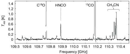
Figure 1: Spectrum near the ${}^{13}$CO and C${}^{18}$O $J=1-0$ lines of W51 e1/e8 taken during the FUGIN survey for calibration purposes.

The sensitivity of the actual FUGIN survey has been set for the ${}^{12}$CO, ${}^{13}$CO and C${}^{18}$O lines, and the resultant rms noise is d$T_{\rm mb}\approx$ 0.2–0.4 K for the ${}^{13}$CO and C${}^{18}$O lines. This makes it difficult to detect hot core tracer lines from the survey data if we depend on only one line of hot core tracer molecule. To improve the signal-to-noise ratio, we stacked the line of HNCO $J_{K_{a},K_{c}}=5_{0,5}-4_{0,4}$ and four lines of CH${}_{3}$CN $J_{K}=6_{K}-5_{K}$ ($K=0,1,2,3$).

In practice, this is still insufficient to efficiently exclude false detections from candidate sources for confirmation observations. Through our preliminary analysis in W51 e1/e8, we found that real sources were always associated with relatively bright C${}^{18}$O emission ($T_{\rm mb}$(C${}^{18}$O) $\geq 1.5$ K), which indicates regions of high column density of molecular gas. Since we can safely assume that hot cores exist in regions of high molecular column density, we require the hot core candidates to be associated with bright C${}^{18}$O emission. We thus selected our candidates in the following three steps:

1. In the C${}^{18}$O datacube, we identify positions with $T_{\rm mb}$(C${}^{18}$O) $\geq$ 1.5 K and record the corresponding peak velocities. By assuming the conditions typical for dense gas, this roughly corresponds to $N{\rm(H_{2})}\geq 8\times 10^{23}$ cm${}^{-2}$.

2. We calculate the integrated intensity of the stacked HNCO and CH${}_{3}$CN lines over $\pm$5 km s${}^{-1}$ centered at the peak velocity of C${}^{18}$O. If the integrated intensity exceeds 5$\sigma$, we regard it as a positive detection.

3. When we find more than two adjacent positive detections in the datacube, we regard them as a single source at the position where we get the strongest integrated intensity of the stacked lines.

We applied this method to the $10^{\circ}\leq l\leq 20^{\circ}$, $-1^{\circ}\leq b\leq 1^{\circ}$ part of the FUGIN data except the three square degrees regions ($12^{\circ}\leq l\leq 13^{\circ}$, $0^{\circ}\leq b\leq 1^{\circ}$; $15^{\circ}\leq l\leq 16^{\circ}$, $0^{\circ}\leq b\leq 1^{\circ}$; and $17^{\circ}\leq l\leq 18^{\circ}$, $0^{\circ}\leq b\leq 1^{\circ}$), which have strong scanning noise and are not suitable for the candidate selection. An rms level of each squared degree is 0.1–0.2 K in the $T_{\rm mb}$ scale as shown in figure 2. We adopted this rms noise levels to calculate the candidate selection threshold in each squared degrees. Consequently, we analyzed the 17 square degrees area of the FUGIN survey following the procedure described above and found 64 candidates for confirmation.

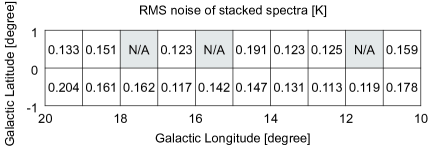
Figure 2: The rms noise levels of the stacked specra at 110 GHz in each squared degrees at 1.3 km s${}^{-1}$ velocity resolution. In three regions (12${}^{\circ}\leq l\leq$13${}^{\circ}$, 0${}^{\circ}\leq b\leq$1${}^{\circ}$; 15${}^{\circ}\leq l\leq$16${}^{\circ}$, 0${}^{\circ}\leq b\leq$1${}^{\circ}$; and 17${}^{\circ}\leq l\leq$18${}^{\circ}$, 0${}^{\circ}\leq b\leq$1${}^{\circ}$), there are strong scanning effect and we did not extract hot core candidates from these regions.

2.2 Confirmation observation

We focus on characteristic chemical abundance of hot core to identify the sources. In addition, we investigate compactness of the molecular distribution to exclude shock-originated molecular lines.

We conducted the observations to hot core candidates using the Nobeyama 45-m radio telescope in 2018 March and May. The 4-beam receiver FOREST ([min16]) and the autocorrelation spectrometer SAM45 ([kun11]) were used. The RF frequency ranges were 94.8–96.8 GHz and 108.8–110.8 GHz in the lower and upper sideband, respectively. The spectrometer was configured to cover 4 GHz in total at a 448.28 kHz channel separation. The corresponding velocity resolution varies from 1.52 km s${}^{-1}$ at 96 GHz to 1.33 km s${}^{-1}$ at 110 GHz. The beam size is $17^{\prime\prime}$ at 96 GHz and $14^{\prime\prime}$ at 110 GHz. The system noise temperatures were 150–350 K at 96 GHz and 200–400 K at 110 GHz during the observations. SiO masers were observed every 1 hour to calibrate the pointing offset of the telescope, and the pointing error was typically less than $3^{\prime\prime}$.

The major spectral lines in the observed frequency ranges are listed in table 2.2. In addition to the C${}^{18}$O $J=1-0$, HNCO $J_{K_{a},K_{c}}=5_{0,5}-4_{0,4}$ and CH${}_{3}$CN $J=6-5$ lines that we used to find the candidates, we observed C${}^{34}$S $J=2-1$, SO $J_{K}=2_{3}-1_{2}$, OCS $J=9-8$, HC${}_{3}$N $J=12-11$, and CH${}_{3}$OH lines, which are often quoted as tracers of hot cores. For CH${}_{3}$OH, in addition to the $J_{K}=2_{0}-1_{0}$ A${}^{+}$, $J_{K}=2_{-1}-1_{-1}$ E and $J_{K}=2_{0}-1_{0}$ E lines, we observed the $J_{K}=8_{0}-7_{1}$ A${}^{+}$ line, which is known to exhibit maser action in some high-mass star forming regions (e.g., [che11]).

List of important molecular lines included in the confirmation observation.
Molecule Transition Frequency [GHz] $E_{\rm u}^{*}/k$ [K] C${}^{18}$O $J=1-0$ 109.782173 005.27 C${}^{34}$S $J=2-1$ 096.412950 006.94 SO $J_{K}=2_{3}-1_{2}$ 109.252220 021.05 OCS $J=9-8$ 109.463063 026.26 HC${}_{3}$N $J=12-11$ 109.173634 034.06 HNCO $J_{K_{a},K_{c}}=5_{0,5}-4_{0,4}$ 109.905749 015.82 CH${}_{3}$CN $J_{K}=6_{0}-5_{0}$ 110.383500 018.54 CH${}_{3}$CN $J_{K}=6_{1}-5_{1}$ 110.381372 025.68 CH${}_{3}$CN $J_{K}=6_{2}-5_{2}$ 110.374989 047.13 CH${}_{3}$CN $J_{K}=6_{3}-5_{3}$ 110.364354 082.85 CH${}_{3}$CN $J_{K}=6_{4}-5_{4}$ 110.349470 132.84 CH${}_{3}$OH $J_{K}=2_{0}-1_{0}$ A${}^{+}$ 096.741371 006.96 CH${}_{3}$OH $J_{K}=2_{-1}-1_{-1}$ E 096.739358 012.54 CH${}_{3}$OH $J_{K}=2_{0}-1_{0}$ E 096.744545 020.09 CH${}_{3}$OH $J_{K}=8_{0}-7_{1}$ A${}^{+}$ 095.169391 083.54 $*$ Upper state energy.

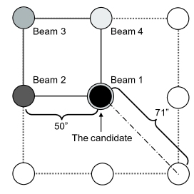
Figure 3: The mapping pattern of the confirmation observation with the FOREST four beams. We observed the candidate at the center with Beam 1, 2, 3 and 4 in turn, so that we can get spectra of the positions $50^{\prime\prime}$ and $71^{\prime\prime}$ away from the center.

We observed the 64 candidates in position switching mode using the FOREST four-beam receiver with the pattern shown in figure 3. The central position of a candidate was observed by the four beams in turn. As a result, we got a $3\times 3$ map with a $50^{\prime\prime}$ grid centered at each candidate. This allows us to judge if the emission is spatially confined ($\ll 100^{\prime\prime}$ = 1.45 pc at 3 kpc) or not, and to exclude extended objects like shocked gas from the hot core candidate list. The integration time was set to achieve a target sensitivity of d$T_{\rm mb}\approx$ 0.03–0.05 K, which was $\sim$ 10 times lower than that of the original FUGIN survey.

3 Results

3.1 Identification of Hot Cores and Dense Clumps

Figure 4 shows an example of the results of our follow-up observations. It shows the line profiles (upper panels) and integrated intensity distributions (lower panels) of the nine important molecular lines observed from one of identified hot core sources, G10.300$-$0.144. For each molecular line, we see its line profile and its spatial extent in a bar graph showing the integrated intensities at the center and the positions $50^{\prime\prime}$ and $71^{\prime\prime}$ away from the center. The intensities at $50^{\prime\prime}$ and $71^{\prime\prime}$ offsets are averages of the intensities at the four positions, i.e., north, south, east and west in the Galactic coordinate at $50^{\prime\prime}$ offset and northeast, northwest, southeast and southwest at $71^{\prime\prime}$ offset, respectively (figure 3). The 1$\sigma$ errors are shown by the solid lines at the top of the bars. The errors shown for the offset positions represent only the statistical errors and do not include the intrinsic intensity variation among the four positions in the average. With exceptions of C${}^{18}$O $J=1-0$ and CH${}_{3}$CN lines, the line intensities are integrated over seven velocity channels ($V_{\rm peak}-4.9$ km s${}^{-1}\leq V_{\rm LSR}\leq V_{\rm peak}+4.9$ km s${}^{-1}$ at 96 GHz and $V_{\rm peak}-4.3$ km s${}^{-1}\leq V_{\rm LSR}\leq V_{\rm peak}+4.3$ km s${}^{-1}$ at 110 GHz) centered at the peak velocity of the C${}^{18}$O emission ($V_{\rm peak}$). The C${}^{18}$O $J=1-0$ line is integrated over 10 channels ($V_{\rm peak}-6.1$ km s${}^{-1}\leq V_{\rm LSR}\leq V_{\rm peak}+6.1$ km s${}^{-1}$). In the case of CH${}_{3}$CN, the strongest $J_{K}=6_{0}-5_{0}$ line is blended with the neighboring $J_{K}=6_{1}-5_{1}$ line, and wider velocity range is used for integration ($V_{\rm peak}-3.7$ km s${}^{-1}\leq V_{\rm LSR}\leq V_{\rm peak}+8.5$ km s${}^{-1}$) to include the $J_{K}=6_{1}-5_{1}$ line.

We regard a line is detected if the integrated intensity exceeds 3$\sigma$ and its profile has a reasonable shape centered at the source velocity defined by the C${}^{18}$O line. The spatial compactness of the molecular emission is judged from a comparison of the integrated intensity at the center with those $50^{\prime\prime}$ and $71^{\prime\prime}$ away. At the distance of 3 kpc, $50^{\prime\prime}$ corresponds to 0.73 pc, which is significantly larger than the typical size of hot cores, detection of hot core tracer lines is expected only toward the center. In the example shown in figure 4, all of the nine molecular lines are detected, and their spatial distribution is compact except for C${}^{18}$O.

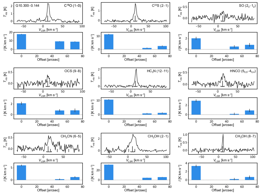
Figure 4: An example of the results of the confirmation observations showing the profiles of nine molecular lines observed from G10.300$-$0.144. Upper part of each panel shows the line profile. The horizontal axis is the radial velocity, $V_{\rm LSR}$ (km s${}^{-1}$), and the vertical axis is the main beam antenna temperature, $T_{\rm mb}$ (K). The long vertical lines indicate the peak velocity of the C${}^{18}$O line, and the short vertical lines for the CH${}_{3}$CN and CH${}_{3}$OH lines correspond to the frequency of their weaker lines. The horizontal lines with ticks on both ends indicate the velocity range of integration. Lower side of each panel shows the integrated intensity of the line at the center, $I=\int T_{\rm mb}\ {\rm d}V$ (K km s${}^{-1}$), and the average intensities at positions $50^{\prime\prime}$ and $71^{\prime\prime}$ away from the center. We can judge the compactness of the emission region by comparison of these three intensities.

The confirmation observation results of the 64 candidates show a range of significance for identification as a hot core. While we detect many of the spectral lines in table 2.2 from some candidates, other sources only show the C${}^{34}$S and CH${}_{3}$OH $J=2-1$ lines besides C${}^{18}$O. Based on the detected lines and their spatial distributions, we classify the candidates into three categories; “Hot Cores”, “Dense Clumps”, and non-detections with the following definitions.

Hot Cores

The sources with detection of at least two of the hot core lines (SO, OCS, HC${}_{3}$N, HNCO, CH${}_{3}$CN and CH${}_{3}$OH $J=8-7$) with clear spatial concentration at the center judged from the comparison of the line intensity at the center with those at positions $50^{\prime\prime}$ and $71^{\prime\prime}$ away from the center. G10.300$-$0.144 shown in figure 4 is a typical example of this category.

Dense Clumps

The sources that fail to meet the Hot Core criteria, but with detection of at least two of C${}^{34}$S, CH${}_{3}$OH $J=2-1$, or the hot core lines listed above.

Non-detections

The candidates that do not meet the criteria for the above two categories are not considered as positive detection. Most of them may represent the inevitable false positive detections in the candidate selection step.

We identified 22 Hot Cores and 14 Dense Clumps, which represent 34% (Hot Cores) and 22% (Dense Clumps) of the observed 64 candidates, respectively. Table 1 shows the identified Hot Cores and Dense Clumps according to the criteria above. Method to estimate distances of each candidate is described in section 3.3. The intensities with the parentheses in table are those below the 3$\sigma$ detection thresholds. Many of the Dense Clumps are detected only in C${}^{34}$S and CH${}_{3}$OH $J=2-1$. We classify G10.203$-$0.341, G10.209$-$0.336, and G12.816$-$0.185 as Dense Clumps despite the multiple detection of hot core lines, because their spatial distributions of the line intensities are not concentrated.

We note that the criteria employed in this work to identify Hot Cores do not explicitly include direct indices of high gas temperature (e.g., $\sim$ 100 K or higher). In this respect, the definition of Hot Cores in this paper may be broader than the classical definition, and the Hot Cores identified here can include also the warm envelopes with similar chemical characteristics that surround forming high-mass stars. An analysis of the excitation temperatures of CH${}_{3}$CN and CH${}_{3}$OH is being planned to further explore this point, but it is outside of the scope of the present paper.

Table 1: Identified Hot Cores and Dense Clumps with integrated intensities

			Integrated intensity [K km s${}^{-1}$]
Name	$V_{\rm{LSR}}$	Distance	C${}^{18}$O	C${}^{34}$S	SO	OCS	HC${}_{3}$N	HNCO	CH${}_{3}$CN	CH${}_{3}$OH	CH${}_{3}$OH
	[km s${}^{-1}$]	[kpc]	$1-0$	$2-1$	$2_{3}-1_{2}$	$9-8$	$12-11$	$5_{0,5}-4_{0,4}$	$6-5$	$2-1$	$8-7$
Hot Cores
G10.145$-$0.339	10.6	3.12 $\pm$0.21	13.49	2.92	1.33	($-0.12$)	(0.02)	1.11	(0.66)	4.88	(0.17)
G10.178$-$0.350	13.3	3.12 $\pm$0.21	23.29	6.49	(0.39)	(0.62)	3.93	1.92	(1.11)	7.14	(0.60)
G10.187$-$0.344	12.0	3.12 $\pm$0.21	22.65	2.09	(0.67)	1.31	1.85	2.91	(1.17)	11.22	(0.22)
G10.220$-$0.369	12.0	3.12 $\pm$0.21	26.02	1.89	(0.27)	(0.77)	1.43	2.43	($-0.11$)	8.53	(0.09)
G10.300$-$0.144	12.0	3.13 $\pm$0.22	17.84	11.46	2.07	2.14	10.61	3.03	6.03	31.53	3.34
G10.465$+$0.034	72.0	8.55 ${}^{+\,0.63}_{-\,0.55}$	11.21	2.27	0.84	(0.49)	1.83	2.99	0.87	12.40	(0.49)
G10.473$+$0.028	66.6	8.55 ${}^{+\,0.63}_{-\,0.55}$	24.07	27.50	11.79	13.28	22.52	14.94	32.48	66.01	14.27
G10.481$+$0.036	66.6	8.55 ${}^{+\,0.63}_{-\,0.55}$	10.92	2.96	1.33	1.51	3.96	6.79	2.92	29.96	2.41
G10.623$-$0.380	$-2.7$:	4.95 ${}^{+\,0.51}_{-\,0.43}$	57.17	33.82	7.01	3.98	25.56	5.66	11.25	39.99	7.84
G11.920$-$0.616	36.0	3.37 ${}^{+\,0.39}_{-\,0.32}$	12.80	4.55	1.24	2.41	8.63	6.12	6.30	39.33	8.76
G11.939$-$0.616	38.6	3.37 ${}^{+\,0.39}_{-\,0.32}$	18.32	7.39	0.65	(0.74)	11.59	1.62	3.77	14.76	1.72
G12.416$+$0.510	18.6	1.83 $\pm$0.09	12.66	3.46	1.10	1.10	4.30	(0.69)	(0.66)	9.49	(0.70)
G12.680$-$0.176	56.0	2.40 ${}^{+\,0.17}_{-\,0.15}$	26.91	2.32	(0.37)	($-0.04$)	2.47	1.49	(0.43)	12.78	(0.45)
G12.810$-$0.204	34.6	2.92 ${}^{+\,0.35}_{-\,0.28}$	48.73	27.96	3.95	2.27	20.78	3.42	5.70	28.83	2.88
G12.888$+$0.490	33.3	2.50 ${}^{+\,0.28}_{-\,0.23}$	27.43	11.42	3.68	2.91	10.92	2.30	5.38	12.96	6.41
G13.185$-$0.109	53.3	4.60 $\pm$0.23	14.81	1.27	(0.26)	($-0.18$)	2.41	1.64	1.54	11.19	(0.38)
G13.199$-$0.134	52.0	4.60 $\pm$0.23	16.17	1.02	(0.10)	(0.42)	0.81	1.55	($-0.37$)	10.03	($-0.22$)
G13.216$+$0.029	52.0	4.57 $\pm$0.22	14.66	1.00	(0.11)	0.80	1.29	1.82	0.93	13.71	0.95
G14.113$-$0.569	21.3	1.86 $\pm$0.10	15.24	2.13	1.60	(0.18)	1.33	(0.67)	1.56	5.02	(0.60)
G14.330$-$0.644	21.3	1.12 ${}^{+\,0.14}_{-\,0.11}$	18.20	12.07	8.60	4.40	22.03	3.41	9.52	50.81	57.76
G14.636$-$0.569	18.6	1.83 ${}^{+\,0.08}_{-\,0.07}$	9.64	2.65	0.48	(0.30)	2.77	0.91	0.91	15.57	1.43
G19.367$-$0.041	26.6	3.11 $\pm$0.26	14.47	2.62	0.48	1.00	0.56	(0.24)	($-0.13$)	10.05	(0.57)
Dense Clumps
G10.131$-$0.408	10.6	3.12 $\pm$0.21	12.69	0.96	(0.00)	($-0.48$)	(0.12)	(0.56)	($-0.28$)	4.60	($-0.08$)
G10.195$-$0.397	10.6	3.12 $\pm$0.21	20.23	1.74	($-0.23$)	($-0.03$)	1.12	(0.74)	(0.03)	5.83	(0.04)
G10.203$-$0.341	12.0	3.12 $\pm$0.21	24.38	1.79	($-0.06$)	(0.90)	(1.07)	0.98	0.58	7.02	(0.43)
G10.203$-$0.308	10.6	3.12 $\pm$0.21	18.60	(0.93)	(0.26)	(0.18)	(0.43)	1.54	(1.10)	2.08	(0.54)
G10.209$-$0.336	12.0	3.12 $\pm$0.21	28.21	1.73	(0.33)	(0.23)	1.67	2.04	(0.32)	7.84	(0.61)
G10.631$-$0.372	$-1.4$:	4.95 ${}^{+\,0.51}_{-\,0.43}$	17.46	3.25	($-0.21$)	(0.43)	2.41	(0.79)	(0.15)	5.73	(0.75)
G11.059$-$0.372	$-1.4$:	4.91 $\pm$0.25	12.70	(0.32)	(0.26)	(0.37)	($-0.06$)	0.83	(0.14)	2.07	($-0.25$)
G11.109$-$0.388	00.0	4.91 $\pm$0.25	10.83	0.55	($-0.12$)	(0.14)	(0.10)	(0.31)	(0.15)	2.82	($-0.02$)
G12.685$-$0.171	54.6	2.40 ${}^{+\,0.17}_{-\,0.15}$	18.89	1.19	($-0.09$)	(0.00)	0.74	0.86	(0.01)	6.18	(0.22)
G12.816$-$0.185	34.6	2.92 ${}^{+\,0.35}_{-\,0.28}$	19.23	5.33	(0.35)	0.72	4.52	2.37	2.31	24.47	1.09
G12.855$-$0.201	36.0	2.92 ${}^{+\,0.35}_{-\,0.28}$	17.08	1.16	($-0.14$)	($-0.21$)	0.78	(0.41)	(0.70)	2.37	($-0.13$)
G12.911$+$0.487	32.0	2.50 ${}^{+\,0.28}_{-\,0.23}$	13.81	1.64	($-0.54$)	(0.00)	(0.81)	(0.79)	($-1.07$)	3.35	(0.64)
G13.202$+$0.057	52.0	4.57 $\pm$0.22	12.17	1.13	(0.16)	($-0.06$)	0.88	(0.68)	(0.82)	2.35	(0.14)
G14.202$-$0.199	38.6	3.09 $\pm$0.39	13.02	1.55	($-0.10$)	(0.04)	(0.14)	(0.34)	(0.93)	8.88	(0.11)

See section 3.3 for the methods of distance determination.
This column shows the integrated intensities of the blend of the CH${}_{3}$CN $J_{K}=6_{0}-5_{0}$ and $J_{K}=6_{1}-5_{1}$ lines.
The column of CH${}_{3}$OH $J=2-1$ shows the integrated intensities of the blend of the $J_{K}=2_{0}-1_{0}$ A${}^{+}$ and $J_{K}=2_{-1}-1_{-1}$ E lines, and the column of CH${}_{3}$OH $J=8-7$ shows the integrated intensities of the $J_{K}=8_{0}-7_{1}$ A${}^{+}$ line.