Efficient Spatially Adaptive Convolution and Correlation

Abstract

Fast methods for convolution and correlation underlie a variety of applications in computer vision and graphics, including efficient filtering, analysis, and simulation. However, standard convolution and correlation are inherently limited to fixed filters: spatial adaptation is impossible without sacrificing efficient computation. In early work, Freeman and Adelson Freeman:PAMI:1991 have shown how steerable filters can address this limitation, providing a way for rotating the filter as it is passed over the signal.

In this work, we provide a general, representation-theoretic, framework that allows for spatially varying linear transformations to be applied to the filter. This framework allows for efficient implementation of extended convolution and correlation for transformation groups such as rotation (in 2D and 3D) and scale, and provides a new interpretation for previous methods including steerable filters and the generalized Hough transform. We present applications to pattern matching, image feature description, vector field visualization, and adaptive image filtering.

Figure 1: Applications of extended convolution. Left: Rotation-independent pattern matching was used to locate the pattern in the image at left. The three correct matches correspond to the three peaks in the match-quality image. Center: A rotation-dependent filter applied to a photograph with added noise produces an artistic effect. Right: Scale-dependent smoothing is used to remove compression artifacts from an image while preserving edges.

1 Introduction

One of the most widely used results in signal processing is the convolution theorem, which states that convolution in the spatial domain is equivalent to multiplication in the frequency domain. Combined with the availability of Fast Fourier Transform algorithms [CT65, FJ05], it reduces the complexity of what would be a quadratic-time operation to a nearly linear-time computation (linearithmic). This, together with the closely-related correlation theorem, have enabled efficient algorithms for applications in many domains, including audio analysis and synthesis [All77, Moo77], pattern recognition and compression of images [KJM05, Wal91], symmetry detection in 2D images [KS06] and 3D models [KFR04], reconstruction of 3D surfaces [SBS06], inversion of the Radon transform for medical imaging [KS01, Nat01], and solving partial differential [Ior01] and fluid dynamic equations [KM90, Sta01].

Despite the pervasiveness of convolution in signal processing, it has an inherent limitation: when convolving a signal with a filter, the filter remains fixed throughout the convolution, and cannot adapt to spatial information.

Early Work on Spatially-Varying Filters

A simple approach to allowing spatial variation is to limit the number of different filters that are allowed. For example, if differently-rotated versions of a filter are required, it is possible to quantize the rotation angle, compute a (relatively) small number of standard convolutions, and select the closest-matching rotation at each pixel.

Motivated by the early research of Knutsson et al. on non-stationary anisotropic filtering Knutsson:TOC:1983, Freeman and Adelson Freeman:PAMI:1991 investigated the idea of steerable filters. The essential observation is that, for angularly band-limited filters, the results of spatially adaptive filtering with arbitrary per-pixel rotation can be computed from per-pixel linear combinations of a finite set of convolutions with rotated filters. Given appropriate conditions on the filter, different transformation groups can be accommodated in this framework [FA91, SF96, THO99].

Contribution

In this work, we provide a representation-theoretic interpretation of steerable filters, and explore generalizations enabled by this interpretation. Our key idea is to focus not on the properties of filters that allow “steerability,” but rather on the structure of the group from which transformations are drawn. Specifically, we show how the ability to perform efficient function steering is related to the decomposition of the space of filters into irreducible representations of the transformation group. The analysis permits us to answer key questions such as:

• How many convolutions are required for spatially-adaptive filtering, given a particular transformation group and a particular filter?

• Given a fixed budget of convolutions, what is the best way to approximate the spatially-adaptive filtering?

We are able to answer these questions not only for 2D rotation, but for a variety of transformations including scaling and non-commutative groups such as 3D rotation. Moreover, we show that it is possible to obtain significantly better approximation results than previous methods that attempt to discretize the space of transformations.

One of our main generalizations is to apply our results to both the convolution and correlation operations, for which the effect of a spatially varying filter has different natural interpretations. Extended convolution is naturally interpreted as a scattering operation, in which the influence of each point in the signal is distributed according to the transformed filter. In contrast, extended correlation has a natural interpretation as a gathering operation, in which each output pixel is the linear combination of input pixels weighted by the locally-transformed filter. We show that the two approaches are appropriate for different applications, in particular demonstrating that the spatially adaptive voting of the Generalized Hough Transform [Bal81] may be implemented using extended convolution with a specially-designed filter.

Figure 1 shows several applications of spatially adaptive filtering that are enabled using our extended correlation and convolution. At left, we show pattern matching that locates all rotated instances of the pattern (top) in the target image (far left). At center we demonstrate an image manipulation in which gradient directions are used to place anisotropic brushstrokes across the image. At right, we show the effect of denoising an image with a filter whose scale is controlled by gradient magnitude, which yields edge-preserving smoothing similar to anisotropic diffusion and bilateral filtering [PM90, Wei97, TM98, Wei06]. For the first two applications, we use spatially adaptive scattering to detect the pattern and to distribute the brushstrokes, respectively. For the third, we use our generalization of function steering to support spatially adaptive (data-dependent) scaling of a smoothing filter.

Approach

Our approach is to leverage the fact that linear transformations of the filter can be realized as invertible matrices acting on a high-dimensional vector space (the space of functions, corresponding to filters). Choosing a basis for the space of functions, the transformation associated to a spatial location can be expressed in matrix form and spatially adaptive filtering can be implemented as a sum of standard convolutions over the matrix entries (Section 3). When the basis is chosen to conform to the irreducible representations of the transformation group, the matrix becomes block-diagonal with repeating diagonal blocks (Section 4), thereby reducing the total number of convolutions that need to be performed.

The generality of the method makes it capable of supporting a number of image processing and image analysis operations. In this paper, we highlight its versatility by describing several of these applications, including the use of the extended convolution in two different types of pattern matching applications (Sections 5, 7, and 6) and three different types of image filtering applications (Section 8). Additionally, we provide a discussion of how filter steering can be generalized to three dimensions, where the group of rotations is no longer commutative (Section 9).

2 Defining Adaptive Filtering

We begin by formalizing our definitions of spatially adaptive filtering. Following the nomenclature of stationary signal processing, we consider both the correlation and convolution of a signal with a filter. Though these operators are identical in the stationary case, up to reflection of the filter through the origin, they define different notions of spatially adaptive filtering.

For both we assume that we are given a spatial function $H$, a filter $F$, and a transformation field ${\mathfrak{T}}$ that defines how the filter is to be transformed at each point in the domain.

2.1 Correlation

The correlation of $H$ with $F$ is defined at a point $p$ as:

$$\bigl{(}H\star F\bigr{)}(p)=\int H(q)\,\overline{F(q-p)}\,dq.$$

Using the notation $\rho_{p}$ to denote the operator that translates functions by the vector $p$:

$$\bigl{(}\rho_{p}F\bigr{)}(q)\equiv F(q-p),$$

we obtain an expression for the correlation as:

$$\bigl{(}H\star F\bigr{)}(p)=\int H(q)\,\overline{\bigl{(}\rho_{p}F\bigr{)}(q)}\,dq.$$

That is, the correlation of $H$ with $F$ can be thought of as a gathering operation in which the value at a point $p$ is defined by first translating $F$ to the point $p$ and then accumulating the values of the conjugate of $F$, weighted by the values of $H$.

We generalize this to spatially adaptive filtering, defining the value of the extended correlation at a point $p$ as the value obtained by first applying the transformation ${\mathfrak{T}}(p)$ to the filter, translating the transformed filter to $p$, and then accumulating the conjugated values of the transformed $F$, weighted by $H$:

$$\{H,\ {\mathfrak{T}}\}\star F=\int H(q)\,\overline{\rho_{p}\bigl{(}{\mathfrak{T}}(p)\,F\bigr{)}(q)}\,dq.$$ (1)

Note that, if the transformations ${\mathfrak{T}}$ are linear, extended correlation maintains standard correlation’s properties of being linear in the signal and conjugate-linear in the filter.

2.2 Convolution

Similarly, convolution can be expressed as:

$$\bigl{(}H*F\bigr{)}(p)=\int H(q)\,\bigl{(}\rho_{q}F\bigr{)}(p)\,dq.$$

In this case, the convolution of $H$ with $F$ can be thought of as a scattering operation, defined by iterating over all points $q$ in the domain, translating $F$ to each point $q$, and distributing the values of $F$ weighted by the value of $H(q)$.

Again, we generalize this to spatially adaptive filtering, defining the extended convolution by iterating over all points $q$ in the domain, applying the transformation ${\mathfrak{T}}(q)$ to the filter $F$, translating the transformed filter to $q$, and then distributing the values of the transformed $F$, weighted by $H(q)$:

$$\{H,{\mathfrak{T}}\}*F=\int H(q)\,\rho_{q}\bigl{(}{\mathfrak{T}}(q)F\bigr{)}(p)\,dq.$$ (2)

Note that, as with standard convolution, the extended convolution is linear in both the signal and the filter (if the transformations ${\mathfrak{T}}$ are linear).

2.3 A Theoretical Distinction

While similar in the case of stationary filters, these operators give rise to different types of image processing techniques in the context of spatially adaptive filtering. This distinction becomes evident if we consider the response of filtering a signal that is the delta function centered at the origin.

In the case of extended convolution, the response is the function ${\mathfrak{T}}(0)\,F$, corresponding to the transformation of the filter by the transformation defined at the origin. In the case of the extended correlation, the response is more complicated: the value at point $p$ comes from the conjugate of the filter at the point(s) $\bigl{(}{\mathfrak{T}}(p)\bigr{)}^{-1}(p)$. Since the transformation field is changing, this implies that some of the values of the filter can be represented by multiple positions in the response, while others might not be represented at all.

Beyond thinking of “gathering” and “scattering,” another way of understanding the distinction between how correlation and convolution extend to varying filters is by considering the dependency of the transformation on the variables. In extended correlation, the filter’s transformation depends on the spatial variable of the result. In contrast, in extended convolution the transformation depends on the variable of integration. This provides another way of deciding which of the operations will be appropriate for a given problem.

2.4 A Practical Distinction

The distinction between the two is also evidenced in a more practical setting, if one compares using steerable filters [FA91] with using the Generalized Hough Transform [Bal81] for pattern detection where a local frame can be assigned to each point.

Steerable Filters

For steerable filters, pattern detection is performed using extended correlation. The filter corresponds to an aligned pattern template, and detection is performed by iterating over the pixels in the image, aligning the filter to the local frame, and gathering the correlation into the pixel. The pixel with the largest correlation value is then identified as the pattern center.

Generalized Hough Transform

For the Generalized Hough Transform, pattern detection is performed using extended convolution. The filter corresponds to candidate offsets for the pattern center and detection is performed by iterating over the pixels in the image, aligning the filter to the local frame, and distributing votes into the candidate centers, weighted by the confidence that the current pixel lies on the pattern. The pixel receiving the largest number of votes is then identified as the pattern center.

3 A First Pass at Adaptive Filtering

In this section, we show that for linear transformations, extended correlations and convolutions can be performed by summing the results of several standard convolutions. If we do not restrict the space of possible transformations, little simplification is possible (either mathematically or in algorithm design) to the brute-force computation implied by Equations 1 and 2. Therefore, we restrict our filter functions to lie within an $n$-dimensional space $\mathcal{F}$, spanned by (possibly complex-valued) basis functions $\langle F_{1},\ldots,F_{n}\rangle$. Moreover, we restrict the transformations ${\mathfrak{T}}(p):\mathcal{F}\rightarrow\mathcal{F}$ to act linearly on functions, meaning that they can be represented with matrices (possibly with complex entries). This permits significant simplification.

We expand the filter as $F=[F_{1}\,\ldots\,F_{n}]\,[a_{1}\,\ldots\,\,a_{n}]^{T}$, and write each transformation ${\mathfrak{T}}(p)$ as a matrix with entries ${\mathfrak{T}}_{ij}(p)$. Thus we can express the transformation of $F$ by ${\mathfrak{T}}(p)$ as the linear combination:

$${\mathfrak{T}}(p)\,F={\mathfrak{T}}(p)\!\left(\sum_{i=1}^{n}a_{i}F_{i}\right)=\sum_{i,j=1}^{n}{\mathfrak{T}}_{ij}(p)\,a_{j}F_{i}.$$

This, in turn, gives an expression for extended correlation as:

$$\bigl{(}\{H,\ {\mathfrak{T}}\}\star F\bigr{)}(p) = \int H(q)\,\overline{\rho_{p}\!\left(\sum_{i,j=1}^{n}{\mathfrak{T}}_{ij}(p)\,a_{j}F_{i}\right)\!(q)}\,dq$$

$$= \sum_{i,j=1}^{n}\overline{{\mathfrak{T}}_{ij}(p)}\int H(q)\,\overline{\rho_{p}\bigl{(}a_{j}F_{i}\bigr{)}(q)}\,dq$$

$$\{H,{\mathfrak{T}}\}\star F = \sum_{i,j=1}^{n}\overline{{\mathfrak{T}}_{ij}}\cdot\left(H\star a_{j}F_{i}\right),$$ (3)

which can be obtained by taking the linear combination of standard correlations. Similarly, we get an expression for extended convolution as:

$$\{H,\ {\mathfrak{T}}\}*F=\sum_{i,j=1}^{n}\left({\mathfrak{T}}_{ij}\cdot H\right)*a_{j}F_{i}$$ (4)

which can also be obtained by taking the linear combination of standard convolutions.

Note that both equations can be further simplified to reduce the total number of standard correlations (resp. convolutions) by leveraging the linearity of the correlation (resp. convolution) operator:

$$\{H,\ {\mathfrak{T}}\}\star F =\sum_{i=1}^{n}\left[\sum_{j=1}^{n}\overline{{\mathfrak{T}}_{ij}a_{j}}\right]\cdot\left(H\star F_{i}\right)$$ (5)

$$\{H,\ {\mathfrak{T}}\}*F =\sum_{i=1}^{n}\left(\left[\sum_{i=1}^{n}{\mathfrak{T}}_{ij}a_{j}\right]\cdot H\right)*F_{i}.$$ (6)

However, we prefer the notation of Equations 3 and 4 as they keep the filter separate from the signal, facilitating the discussion in the next section.

Example $n=1$

As a simple example, we consider the case in which we would like to correlate a signal with an adaptively rotating filter $F$ which is supported within the unit disk and has values:

$$F(r,\theta)=ae^{ik\theta}.$$

In this case, rotating by an angle $\Theta$ amounts to multiplying the filter by $e^{-ik\Theta}$. Thus, the extended correlation at point $p$ can be computed by multiplying the filter $F$ by $e^{-ik\Theta(p)}$, where $\Theta(p)$ is the angle of rotation at $p$, and then evaluating the correlation with the transformed filter at $p$. However, since correlation is conjugate-linear in the filter, the value of the extended correlation can also be obtained by first performing a correlation of $H$ with the un-transformed $F$, and only then multiplying the result at point $p$ by $e^{ik\Theta(p)}$.

Example $n=3$

Next, we consider a more complicated example in which the filter $F$ resides within a three-dimensional space of functions, $F=a_{1}F_{1}+a_{2}F_{2}+a_{3}F_{3}$, with the basis defined as:

$$F_{1}(r,\theta)=e^{i2\theta},\quad F_{2}(r,\theta)=e^{-i2\theta},\quad F_{3}(r,\theta)=1$$

In this case, rotating by an angle $\Theta$ amounts to multiplying the first component of the filter by $e^{-i2\Theta}$, the second by $e^{i2\Theta}$, and the third by $1$ so the previous approach will not work. However, by linearity, the extended correlation with $F$ can be expressed as the sum of the separate extended correlations with $aF_{1}$, $bF_{2}$, and $cF_{3}$. Each of these can each be obtained by computing the standard correlations with $a_{1}F_{1}$, $a_{2}F_{2}$, and $a_{3}F_{3}$ and then multiplying the values at point $p$ by $e^{i2\Theta(p)}$, $e^{-i2\Theta(p)}$, and $1$ respectively. Thus, we can obtain the extended correlation by performing $n=3$ separate correlations and taking their linear combination.

With respect to the notation in Equation 3, rotating the filter $F$ by an angle of $\Theta$ multiplies the coefficients $(a_{1},a_{2},a_{3})^{T}$ by:

$${\mathfrak{T}}_{ij}(\Theta)=\left(\begin{array}[]{ccc}e^{-i2\Theta}&0&0\\ 0&e^{i2\Theta}&0\\ 0&0&1\end{array}\right).$$

Thus, the extended correlation with $F$ can be computed by computing the standard correlations with the $n^{2}=9$ functions $a_{i}F_{j}$, multiplying the results of these correlations by the functions ${\mathfrak{T}}_{ij}(p)$, and then taking the sum. However, since the functions ${\mathfrak{T}}_{ij}(p)$ are uniformly zero whenever $i\neq j$, the standard correlations with $a_{i}F_{j}$ become unnecessary for $i\neq j$, and the extended correlation can be expressed using only $n=3$ standard correlations.

Example $n=3$, revisited

Though the previous example shows that the extended correlation with $F$ can be computed efficiently, we now show that the efficiency is tied to the way in which we factored the filter. In particular, we show that if the wrong factorization is chosen, the cost of computing the extended correlation can increase. Consider the same filter as above, but now expressed as the linear combination of a different basis as $F(r,\theta)=\tilde{a}_{1}\tilde{F}_{1}(r,\theta)+\tilde{a}_{2}\tilde{F}_{2}(r,\theta)+\tilde{a}_{3}\tilde{F}_{3}(r,\theta)$, with:

$$\tilde{F}_{1}(r,\theta)=\cos^{2}\!\theta,~{}~{}\tilde{F}_{2}(r,\theta)=\sin^{2}\!\theta,~{}~{}\tilde{F}_{3}(r,\theta)=\cos\theta\sin\theta.$$

Rotating such a filter by an angle of $\Theta$ multiplies the coefficients $(\tilde{a}_{1},\tilde{a}_{2},\tilde{a}_{3})^{T}$ by:

$$\tilde{{\mathfrak{T}}}_{ij}(\Theta)=\left(\begin{array}[]{ccc}\cos^{2}\Theta&\phantom{-}\sin^{2}\Theta&-\cos\Theta\sin\Theta\\ \sin^{2}\Theta&\phantom{-}\cos^{2}\Theta&\phantom{-}\cos\Theta\sin\Theta\\ \sin 2\Theta&-\sin 2\Theta&\cos 2\Theta\end{array}\right).$$

Thus, the extended correlation with $F$ can be computed by computing the standard correlations with the functions $\tilde{a}_{i}\tilde{F}_{j}$, multiplying the results of these correlations by the functions $\tilde{{\mathfrak{T}}}_{ij}(p)$ respectively, and then taking the sum. In this case, since the matrix entries are all non-zero, all $n^{2}=9$ standard correlations are required.

Of course, the above discussion was purely a strawman: using the grouping of terms in Equations 5 and 6, it is possible to avoid the need for $n^{2}$ correlations. However, focusing on the structure of the ${\mathfrak{T}}$ matrix and using the tools of representation theory to find a basis in which it has a particularly simple structure, we can bring the computational requirements even below $O(n)$ correlations or convolutions.

4 Choosing a Basis

As hinted at in the previous section, the efficiency of the implementation of extended correlation (resp. convolution) is tied to the choice of basis. In this section we make this explicit by showing that by choosing the basis of functions appropriately, we obtain matrices that are sparse (with many zero entries) and have repeated elements. Each zero and repetition corresponds to a standard correlation (resp. convolution) that does not need to be computed.

We begin by considering the group of planar rotations. We show that there exists a basis of functions in which the transformation matrix ${\mathfrak{T}}$ becomes sparse, specifically diagonal. We then use results from representation theory to generalize this, and to establish limits on how sparse the matrix ${\mathfrak{T}}$ can be made. We conclude this section with a detailed discussion of the relation of our work to earlier work in steerable functions.

4.1 Rotations

To motivate the result that the choice of basis is significant to the structure of the matrix ${\mathfrak{T}}$, consider planar rotations and their effect on 2D functions. In this case, the structure of ${\mathfrak{T}}$ is most easily exposed by considering the filter in polar coordinates. In particular, rotations preserve radius: $(r,\theta)$ is necessarily mapped to $(r,\theta^{\prime})$. Thus, in polar coordinates the only nonzero entries in ${\mathfrak{T}}$ occur in blocks around the diagonal, one block for each $r$. Starting with an $n$-pixel image, transformation into polar coordinates will give a function sampled at $N=O(n^{1/2})$ radii and $K=O(n^{1/2})$ angles. Hence the nonzero entries in ${\mathfrak{T}}$ will occupy $N$ blocks of size $K\times K$.

To make ${\mathfrak{T}}$ even more sparse, we consider representing the functions at each radius in the frequency domain, rather than the spatial domain. That is, within a radius the basis functions are proportional to $e^{ik\theta}$, for a fixed $k$. Applying a rotation to such a single-frequency function preserves that frequency; it is, in fact, expressible by multiplying the function by $e^{-ik\Theta}$, where $\Theta$ is the angle of the rotation. Therefore, in this basis ${\mathfrak{T}}$ has been simplified to purely diagonal (with complex entries).

In moving from an arbitrary basis to polar and polar/Fourier bases, we have reduced the number of nonzero entries in ${\mathfrak{T}}$ from $(N\times K)^{2}=O(n^{2})$ to $N\times K^{2}=O(n^{1.5})$ to $N\times K=O(n)$. Correspondingly, the number of standard correlations (resp. convolutions) that need to be computed is also reduced.

There is one more reduction we may obtain by considering repeated entries in ${\mathfrak{T}}$. In particular, we observe that all the diagonal entries corresponding to a particular frequency $k$, across different radii, will be the same: $e^{-ik\Theta(p)}$. Although the rotation angle $\Theta(p)$ may vary across the image, all of these entries will vary in lock-step, and the associated diagonal entries ${\mathfrak{T}}_{ii}$ will be identical. Thus, we may perform all such correlations (resp. convolutions) at once by correlating (resp. convolving) $e^{-ik\Theta(q)}$ with the sum of all $a_{i}F_{i}$, where $F_{i}$ has angular frequency $k$. As a result, the number of distinct correlations (resp. convolutions) is reduced to $K=O(n^{1/2})$.

Summarizing, to compute the extended correlation of a 2D signal $H$ and rotation field ${\mathfrak{T}}$ with filter $F$:

Filter Decomposition

We first decompose $F$ as the sum of functions with differing angular frequencies:

$$F=\sum_{k=-K/2}^{K/2}F_{k}\qquad\hbox{with}\qquad F_{k}(r,\theta)=f_{k}(r)\,e^{ik\theta}.$$

This can be done, for example, by first expressing $F$ in polar coordinates, and then running the 1D FFT at each radius to get the different frequency coefficients. [$O(n+n\log n)$]

Standard Correlation

Next, we compute the standard correlations of the signal with the functions $F_{k}(r,\theta)=f_{k}(r)e^{ik\theta}$:

$$G_{k}=H\star F_{k}\qquad\hbox{for each }k\in[-K/2,K/2].$$

This can be done by first evaluating the function $f_{k}(r)e^{ik\theta}$ on a regular grid and then using the 2D Fast Fourier Transform to perform the correlation. [$O(n^{3/2}+n^{3/2}\log n)$]

Linear Combination

Finally, we take the linear combination of the correlation results:

$$\bigl{(}\{H,\ {\mathfrak{T}}\}\star F\bigr{)}(p)=\sum_{k=-K/2}^{K/2}e^{ik\Theta(p)}\,G_{k}(p),$$

weighting the contribution of the $k$-th correlation to the pixel $p$ by the conjugate of the $k$-th power of the unit complex number corresponding to the rotation at $p$. [$O(n^{3/2})$]

The extended convolution can be implemented similarly, but in this case we need to pre-multiply the signal:

$$G_{k}(p)=H(p)\cdot e^{-ik\Theta(p)}\qquad\hbox{for each }k\in[-K/2,K/2]$$

and only then sum the convolutions of $G_{k}$ with $F_{k}$.

4.2 Generalization

In implementing the extended correlation for rotations we have taken advantage of the fact that the space of filters could be expressed as the direct-sum of subspaces that (1) are fixed under rotation, and (2) could be grouped into subspaces on which rotations act in a similar manner.

The decomposition of a space of functions into such subspaces is a central task of representation theory, which tells us that any vector-space $V$, acted upon by a group $G$, can be decomposed into a sum of subspaces (e.g. [Ser77]):

$$V\cong\,\bigoplus_{\lambda}\,m_{\lambda}\!V^{\lambda},$$

where $\lambda$ is the frequency, indexing the subspace fixed under the action of the group, and $m_{\lambda}$ is the multiplicity of the subspace. While we are only guaranteed that the subspace $V^{\lambda}$ is one-dimensional when the group $G$ is commutative, the subspace $V^{\lambda}$ is guaranteed to be as small as possible (i.e. irreducible) so that $V^{\lambda}$ cannot be decomposed further into subspaces fixed under the action of $G$.

Using the decomposition theorem, we know that if ${\mathcal{F}}$ represents the space of filters and the transformations ${\mathfrak{T}}(p)$ belong to a group $G$, then we can decompose ${\mathcal{F}}$ into irreducible representations of $G$:

$${\mathcal{F}}=\,\bigoplus_{k=1}^{\gamma}\left(\bigoplus_{l=1}^{m_{k}}{\mathcal{F}}_{kl}\right)$$ (7)

where $k$ indexes the sub-representation and, for a fixed $k$, the sub-representations $\left\{{\mathcal{F}}_{kl}\right\}_{l=1}^{m_{k}}$ are all isomorphic.

Referring back to the discussion of rotation in Section 4.1, the group acting on the filters is $G=\textrm{SO}(2)$ (the group of rotations in the plane) and the sub-representations ${\mathcal{F}}_{kl}$ are just functions of constant radius and constant angular frequency.

4.2.1 Block-Diagonal Matrix

Using the decomposition in Equation 7, we can choose a basis for ${\mathcal{F}}$ by choosing a basis for each subspace ${\mathcal{F}}_{kl}$. Since for fixed $k$ the $\{{\mathcal{F}}_{kl}\}_{l=1}^{m_{k}}$ are all isomorphic, we can denote their dimension by $n_{k}$ and represent the basis for ${\mathcal{F}}_{kl}$ by:

$${\mathcal{F}}_{kl}=\hbox{Span}\langle F_{1}^{kl},\ldots,F_{n_{k}}^{kl}\rangle.$$

Additionally, since ${\mathcal{F}}_{kl}$ is a sub-representation, we know that ${\mathfrak{T}}(q)$ maps ${\mathcal{F}}_{kl}$ back into itself. This implies that we can represent the restriction of ${\mathfrak{T}}(q)$ to ${\mathcal{F}}_{kl}$ by an $n_{k}\times n_{k}$ matrix with $(i,j)$-th entry ${\mathfrak{T}}_{ij}^{kl}(q)$. Thus, given $F=\sum a_{i}^{kl}F_{i}^{kl}\in{\mathcal{F}}$, we can express the transformation of $F$ by ${\mathfrak{T}}(q)$ as:

$${\mathfrak{T}}(q)(F)=\!\sum_{k=1}^{{\gamma}_{\vrule width=0.0pt,height=3.7pt,depth=0.0pt}}\sum_{l=1}^{\,m_{k}}\sum_{i,j=1}^{n_{k}}{\mathfrak{T}}_{ij}^{kl}(q)\,a_{i}^{kl}F_{j}^{kl}$$

corresponding to a block-diagonal representation of ${\mathfrak{T}}$ by a matrix with $\sum m_{k}$ blocks, where the $(k,l)$-th block is of size $n_{k}\times n_{k}$. As before, this gives:

$$\{H,\ {\mathfrak{T}}\}\star F=\!\sum_{k=1}^{{\gamma}_{\vrule width=0.0pt,height=3.7pt,depth=0.0pt}}\sum_{l=1}^{\,m_{k}}\sum_{i,j=1}^{n_{k}}\overline{{\mathfrak{T}}_{ij}^{kl}}\cdot\left(H\star a_{i}^{kl}F_{j}^{kl}\right).$$

Using this decomposition, evaluating the extended correlation now requires the computation of $m_{1}n_{1}^{2}+\cdots+m_{R}\,n_{R}^{2}$ standard correlations. Note that, since $n=m_{1}n_{1}+\cdots+m_{R}\,n_{R}$, the number of linear combinations will be smaller than $n^{2}$ if the space ${\mathcal{F}}$ contains more than one irreducible representation.

4.2.2 Multiplicity of Representations

We further improve the efficiency of the extended correlation by using the multiplicity of the representations. Since the spaces $\{{\mathcal{F}}_{kl}\}_{l=1}^{m_{k}}$ correspond to the same representation, we can choose bases for them such that the matrix entries ${\mathfrak{T}}_{ij}^{kl}(q)$ have the property that ${\mathfrak{T}}_{ij}^{kl}(q)={\mathfrak{T}}_{ij}^{kl^{\prime}}(q)\equiv{\mathfrak{T}}_{ij}^{k}$ for all $1\leq l,l^{\prime}\leq m_{k}$. As a result, the extended correlation simplifies to:

$$\{H,\ {\mathfrak{T}}\}\star F=\!\sum_{k=1}^{{\gamma}_{\vrule width=0.0pt,height=3.7pt,depth=0.0pt}}\sum_{i,j=1}^{n_{k}}\Biggl{[}\overline{{\mathfrak{T}}_{ij}^{k}}\cdot\left(H\star\biggl{[}\sum_{l=1}^{\,m_{k}}a_{i}^{kl}F_{j}^{kl}\!\biggr{]}\right)\Biggr{]}.$$

Thus, we only need to perform one standard correlation for each set of isomorphic representations, further reducing the number of standard correlations to $n_{1}^{2}+\cdots+n_{R}^{2}$.

While the previous discussion has focused on the extended correlation, an analogous argument shows that the same decomposition of the space of filters results in an implementation of the extended convolution that requires $n_{1}^{2}+\cdots+n_{R}^{2}$ standard convolutions.

4.3 Band-Limiting

In practice, we approximate the extended correlation (resp. convolution) by only summing the contribution from the first $K\ll{\gamma}$ frequencies, for some constant $K$. This further reduces the number of standard correlations (resp. convolutions) to $n_{1}^{2}+\cdots+n_{K}^{2}$ and is equivalent to band-limiting the filter prior to the computation of the extended convolution. For example, when rotating images sampled on a regular grid with $n$ pixels, this can reduce the complexity of extended correlation to $O(K\,n\log n)$ by band-limiting the filter’s angular components.

4.4 Relation to Steerable Filters

Using the extended correlation, the method described above can be used to perform efficient steerable filtering. While the implementation differs from the one described in [FA91], the complexity is identical, with both implementations running in $O(K\,N^{2}\log N)$ time for $N\times N$ images and filters with maximal angular frequency $K$.

We briefly review Freeman and Adelson’s implementation of steerable filtering and discuss how it fits into our representation-theoretic framework. We defer the discussion of the limitations of the earlier implementation in the context of higher-dimensional steering to Section 9.

In the traditional implementation of steerable filters, the filter $F$ is used to define the steering basis. (Note that the original work of Freeman and Adelson Freeman:PAMI:1991 also proposes, but does not use, an interpretation based on alternative basis functions.) Specifically, when the filter is angularly band-limited with frequency $K$, the steerable filtering is performed using the functions $F_{0},\ldots,F_{K-1}$, where the function $F_{k}$ is the rotation of $F$ by an angle of $k\pi/K$.

Because the span of these functions is closed under rotation and because it contains the filter $F$, the functions $F_{0},\ldots,F_{K-1}$ can be used for performing the extended correlation. In particular, one can compute the matrix ${\mathfrak{T}}_{ij}(\Theta)$ describing how the rotation of a basis function can be expressed as a linear combination of the basis, and then take the linear combinations of the standard correlations of the signal with the functions $a_{j}F_{i}$ weighted by the matrix entries ${\mathfrak{T}}_{ij}$.

While this interpretation of steerable filtering within the context of our representation-theoretic framework hints at an implementation requiring $K^{2}$ standard correlations (since the entries ${\mathfrak{T}}_{ij}$ are non-zero) this is not actually the case. What makes the classical implementation of steerable filtering efficient is that the filter is one of the basis vectors, $F=F_{0}$, so the decomposition of the filter $F$ as $F=a_{0}F_{0}+\cdots+a_{K-1}F_{K-1}$, has $a_{0}=1$ and $a_{i}=0$ for all $i\neq 0$. Thus, while all $K^{2}$ matrix entries ${\mathfrak{T}}_{ij}$ are non-zero, only $K$ of the functions $a_{j}F_{i}$ are non-zero, so the steerable filtering only requires that $K$ standard correlations be performed.

5 Application to Pattern Detection

We apply extended convolution to detect instances of a pattern within an image, even if the pattern occurs at different orientations. Recall that this approach may be thought of as an instance of the generalized Hough transform, such that image pixels vote for locations consistent with the presence of the pattern. Figure 1, left, shows an example application in which we search for instances of a pattern in Escher’s Heaven and Hell. In this example, all three rotated versions of the pattern give a high response.

5.1 Defining the Filter and Transformation Field

Our strategy will be to operate on the gradients of both the pattern $P$ and the target image $I$. In particular, we take the signal to be

$$H=\bigl{\|}\nabla I\bigr{\|},$$ (8)

and the transformation field ${\mathfrak{T}}$ to be rotation by the angle $\theta$, where

$$\theta_{\nabla I}=\textrm{atan2}\left(\frac{\partial I}{\partial y},\ \frac{\partial I}{\partial x}\right)$$ (9)

and atan2 is the usual two-argument arctangent function.

To design the filter $F$, we consider what will happen during the extended convolution when we place $F$ at some pixel $q$. The values of $F$ will be scattered, with weight proportional to the gradient magnitude at $q$; in other words, the filter will have its greatest effect at edges in the target image. Now, if $q$ were the only point with non-zero gradient magnitude, the optimal filter $F$ would simply be the distribution that scatters all of its mass to the single point $\widetilde{p}$ – the pattern center relative to the coordinate frame at $q$. When there are multiple points with non-zero gradient magnitude, we set $F$ to be the “consensus filter”, obtained by taking the linear combination of the different distributions, with weights given by the gradient magnitudes.

Figure 2: Visualization of the construction of the optimal filter defined in Equation (10): A crop from an input image is shown on the left. The gradients, the keypoint $p$, and neighboring points $q_{i}$ are shown in the middle. The derived filter is shown on the right.

In practice, the filter is itself constructed by a voting operation. For example, consider Figure 2, which shows an example of constructing the optimal filter (right) for an ‘A’ pattern (left) with respect to its gradient field (middle) at the point $p$. For each point $q$ in the vicinity of the pattern’s center, the gradient determines both the position of the bin and the weight of the vote with which $q$ contributes to the filter. For example, since the gradient at $q_{1}$ is interpreted as the $x$-axis of a frame centered at $q_{1}$, the position of $p$ relative to this frame will have negative $x$- and $y$-coordinates. The gradient at $q_{1}$ has a large magnitude, so the point $q_{1}$ contributes a large vote to bin $\widetilde{p}_{1}$. The keypoint $p$ has positive $x$- and $y$-coordinates relative to the frame at $q_{3}$ but since the gradient is small, it contributes a lesser vote to bin $\widetilde{p}_{3}$.

Iterating over all points in the neighborhood of the pattern’s center, we obtain the filter shown on the right. While the filter does not visually resemble the initial pattern, several properties of the pattern can be identified. For example, since the gradients along the outer left and right sides of the ‘A’ tend to be outward facing, points on these edges cast votes into bins with negative $x$-coordinates, corresponding to the two vertical seams on the left side of the filter. Similarly, the gradients on the inner edges point inwards, producing the small wing-like structures on the right side of the filter.

Formally, we define the filter as:

$$F=\int\|\nabla P\|\ \rho_{-{\mathfrak{T}}^{-1}(q)\cdot(p-q)}\ \delta\ dq,$$ (10)

where the transformation field ${\mathfrak{T}}$ is defined as rotation by the gradient directions of the pattern $P$, and $\delta$ is the unit impulse, or Dirac delta function. This encapsulates the voting strategy described above. In the appendix, we show that the filter $F$ defined in this manner optimizes the response of the extended convolution at the origin.

5.2 Discussion: Band-Limiting Revisited

As we have seen, the extended convolution of an $N\times N$ image with a rotating filter can be computed in $O(N^{3}\log N)$ time by computing $O(N)$ standard convolutions. Though this is faster than the $O(N^{4})$ brute force approach, a similar form of pattern matching could be implemented in $O(N^{3}\log N)$ by generating $O(N)$ rotations of the filter, performing a convolution of the image with each one, and setting the value of the response to be the maximum of the responses over all rotations.

The difference becomes apparent when we consider limiting the number of convolutions. As an example, Figure 3, top, shows the results of extended convolution-based pattern detection using low order frequencies. The band-limiting in the angular component gives blurred versions of the match-strength image, with the amount of blur reduced as the number of convolutions is increased. In contrast, convolving the image with multiple rotations of the pattern, as shown in the middle row, yields sub-sampled approximations to the response image, and more standard convolutions are required in order to reliably find all instances of the pattern. We can actually make a specific statement: the best way (in the least-squares sense, averaged over all possible rotations) to approximate the ideal extended convolution with a specific number of standard convolutions is to use the ones corresponding to the largest $a_{i}$: the most important projections onto the rotational-Fourier basis. Since in practice the lowest frequencies have the highest coefficients, simply using the lowest few bases is a useful heuristic.

Figure 3: Comparison of approximations to exact pattern detection. Using subsets of frequencies for extended convolution (top) converges more quickly than convolution with multiple rotations of the pattern (bottom).

6 Application to Contour Matching

As a second test, we apply extended convolution to the problem of matching complementary planar curves. To generate the signal and the rotation field, we rasterize the contour lines and their normals into a regular grid. We further convolve both the signal and the vector field with a narrow Gaussian to extend the support of the functions. Using these, we can define filters for queries and compute extended convolutions.

Our contour matching algorithm differs from standard pattern matching in two ways. First, we are searching for complementary shapes, not matching ones. Using the fact that complementary shapes have similar local signals, but oppositely oriented gradient fields, we define the filter using the negative of the query contour’s gradient field. Additionally, after finding the optimal aligning translation using extended convolution, we perform an angular correlation to find the rotation minimizing the $L_{2}$-difference between query and target.

An example search is shown in Figure 4. The image on the left shows the query contour, with a black circle indicating the region of interest. The image on the right shows the top nine candidate matches returned using the extended convolution, sorted by retrieval rank from left to right and top to bottom. Blue dots show the best matching position as returned by the extended convolution, and the complete transformation is visualized by showing the registered position of the query in the coordinate system of the target. Note that even for pairs of contours that do not match, our algorithm still finds meaningful candidate alignments.

Figure 4: An example of applying the extended convolution to contour matching. The image on the left shows the query contour with the region of interest selected. The images on the right show the best nine candidate matches returned by our system, in sorted order.

To evaluate our matching approach, we applied it to the contours of fragmented objects. Reconstructing broken artifacts from a large collection of fragments is a labor-intensive task in archeology and other fields, and the problem has motivated recent research in pattern recognition and computer graphics [MK03, HFG^∗06, BTFN^∗08]. As a basis for our experiments, we used the ceramic-3 test dataset that is widely distributed by Leitão and Stolfi Stolfi:TPAMI:2002. This dataset consists of 112 two-dimensional fragment contours that were generated by fracturing five ceramic tiles, and then digitizing the pieces on a flatbed scanner and extracting their boundary outlines.

Running the contour matching algorithm on each pair of fragments produces a sorted list of the top candidate matching configurations for each fragment pair. These candidate matches are reviewed to verify if they correspond to a true match. By using the same dataset, we can directly compare our algorithm’s performance against the multiscale dynamic programming sequence matching algorithm and results described in [LS02]. We used the same contour sampling resolution as their finest multiresolution scale: fragments thus ranged from 690 to 4660 samples per contour. The numbers of true matches found within the first $n$ ranked candidate matches found by the two algorithms are compared in Figure 5.

The extended convolution matching algorithm outperforms the multiscale sequence matching algorithm, and finds 72% more correct matches among the top-ranked 277 candidates. At this level of matching precision, our algorithm requires 6 hours to process the entire dataset of 112 fragments on a desktop PC (3.2 GHz Pentium 4). By reducing the sampling rate of the contour line rasterization grid or increasing the step size along the contours between extended convolution queries, the running time can be reduced significantly while trading off some search precision. For collections with a large number of fragments, the matching algorithm can easily be executed in parallel on subsets of the fragment pairs.

Figure 5: The number of true contour matches within the first $n$ ranked candidate matches found using extended convolution, as compared to those found using method of Leitão and Stolfi.

7 Application to Image Matching

An image feature descriptor can be constructed from the discretization of the optimal filter $F$, as defined in Equation (10), relative to the signal and frame field in Equations (8) and (9). We call this descriptor the Extended Convolution Descriptor (ECD).

We compare the ECD image descriptor against SIFT in the context of feature matching on a challenging, large-scale dataset. We choose to compare against SIFT for several reasons. Foremost, SIFT has stood the test of time. Despite its introduction over two decades ago, SIFT is arguably the premier detection and description pipeline and remains widely used across a number of fields, including robotics, vision, and medical imaging. Competing pipelines have generally emphasized computational efficiency and have yet to definitively outperform SIFT in terms of discriminative power and robustness[KPS17, TS18].

The advent of deep learning in imaging and vision has coincided with the introduction of a number of contemporaneous learned descriptors which have been shown to significantly outperform SIFT and other traditional methods in certain applications[MMRM17, HLS18, LSZ^∗18, ZR19]. However, the performance of learned descriptors is often domain-dependent and “deterministic" descriptors such as SIFT can provide either comparable or superior performance in specialized domains that learned descriptors are not specifically designed to handle[ZFR19]. More generally, “classical" methods for image alignment and 3D reconstruction, e.g. SIFT + RANSAC, may still outperform state-of-the-art learned approaches with the proper settings[SHSP17, JMM^∗20]. It is also worth noting that the extended convolution can be written as a convolution on $\textrm{SE}(2)$ (the group of planar rigid motions) by introducing Dirac delta functions to restrict contributions of integral over $\textrm{SO}(2)$ to those orientations defined by transformation field. Similar approaches have been shown to be an effective basis for image template matching [KC99a, KC99b, CK16].

The scope of this work is limited to local image descriptors – we do not consider the related problem of feature detection. The SIFT pipeline integrates both feature detection and description in the sense that keypoints are chosen based on the distinctive potential of the surrounding area. As we seek to compare against the SIFT descriptor directly, we perform two sets of experiments. In the first, we replace the SIFT descriptor with ECD within the SIFT pipeline to compare practical effectiveness. The goal of the second experiment is to more directly evaluate our contribution with respect to the design of rotationally invariant descriptors. Specifically, we seek an answer to the following question: By having all points in the local region encode the keypoint relative to their own frames, do we produce a more robust and discriminating descriptor than one constructed relative to the keypoint’s frame?

7.1 Comparison Regime

In both sets of experiments, we evaluate ECD and SIFT in the context of descriptor matching using the publicly available photo-tourism dataset associated with the 2020 CVPR Image Matching Workshop[JMM^∗20]. The dataset consists of collections of images of international landmarks captured in a wide range of conditions using different devices. As such, we use the dataset to simultaneously evaluate descriptiveness and robustness. The dataset also includes 3D ground-truth information in the form of the camera poses and depth maps corresponding to each image. In all of our experiments, we use the implementation of SIFT in the OpenCV library[Bra00] with the default parameters.

Due to the large size of the dataset, we restrict our evaluations to the image pools corresponding to six landmarks: reichstag, pantheon_exterior, sacre_coeur, taj_mahal, temple_nara_japan, and westminster_abbey, which we believe reflect the diversity of the dataset as a whole. Experiments are performed by evaluating the performance of the descriptors in matching a set of scene images to a smaller set of models.

For each landmark, five model images are chosen and removed from the pool. These images are picked such that their subjects overlap but differ significantly in terms of viewpoint and image quality. The scenes are those images in the remainder of the pool that best match the models.

Specifically, SIFT keypoints are computed for all model in each pool. Keypoints without a valid depth measure are discarded. For each landmark, images in the pool are assigned a score based on the number of keypoints that are determined to correspond to at least one keypoint from the five models originally drawn from the pool.

Keypoints are considered to be in correspondence if the distance between their associated 3D points is less than a threshold value $\tau$. For each of the five models, all pixels with valid depth are projected into 3D using the ground-truth depth maps and camera poses. These points are used to compute a rough triangulation corresponding to the surface of the landmark. As in [GBS^∗16], we define the threshold value relative to the area of the mesh, $A$,

$$\tau=0.005\cdot\sqrt{A\ /\ \pi\ }.$$ (11)

The top 15 images with the highest score from each pool are chosen as the scenes. The scaling factor in the value of $\tau$ was determined empirically; it provides a good balance between keypoint distinctiveness and ensuring each scene contributes approximately 1000 keypoints to the total.

Comparisons within the SIFT Pipeline

(a) Keypoints and scale determined by the SIFT feature detector

(b) Randomly selected keypoints and scale estimated from ground truth

Figure 6: The mean precision-recall curves for the ECD and SIFT descriptors. On the left, the keypoints and corresponding scales are computed in the SIFT pipeline. The three different curves correspond to the average over all scenes using the first 200, 500, and 1000 keypoints in each. On the right, keypoints are selected at random and scale is estimated from the ground truth. The curves are averaged over all scenes using 1000 keypoints in each.

In our first experiment, we perform comparisons with keypoints selected using the SIFT keypoint detector to gauge ECD’s practical effectiveness. For each model, we compute SIFT keypoints and sort them in descending order by “contrast”[Low04]. Of these, we retain the first 1000 distinct keypoints having a valid depth measure, preventing models with relatively large numbers of SIFT keypoints from having an outsize influence in our comparisons.

For each scene, we compute SIFT keypoints and discard those without valid depth. Those that remain are sorted by contrast and only the first 1000 distinct keypoints that match at least one keypoint from the five corresponding models are retained.

Next, ECD and SIFT descriptors are computed at each keypoint for both the models and the scenes. Both descriptors are computed at the location in the Gaussian pyramid assigned to the keypoint in the SIFT pipeline. The support radius, $\epsilon$, of the SIFT descriptor is determined by the scale associated with the keypoint in addition to the number of bins used in the histogram. The ECD descriptor uses more bins and we find that it generally exhibits better performance using a support radius 2.5 times larger that of the corresponding SIFT descriptor.

Comparisons using Randomized Keypoints

Our second set of experiments are performed in the same manner using the same collection of models and scenes. The only difference is that the keypoints are selected at random so as to avoid the influence of the SIFT feature detection algorithm on the results. Specifically, for each model, 1000 keypoints are randomly chosen out of the collection of points that have a valid depth measure. Then, for each scene, we randomly select keypoints with valid depth and keep only those that correspond to at least one keypoint from the five associated images in the models. This process is iterated until 1000 such points are obtained.

We use the ground-truth 3D information to provide an idealized estimation of the scale. That is, for a keypoint, the associated 3D point is first translated by $2\tau$ in a direction perpendicular to the camera’s view direction and then projected into the image plane. For both descriptors, the distance between the 2D keypoint and the projected offset defines the support radius.

Evaluating Matching Performance

In both sets of experiments, we evaluate the matching performance of the SIFT and ECD descriptors by computing precision-recall curves for all keypoints in the scenes, an approach that has been demonstrated to be well-suited to this task[KS04, MS05]. Given a scene keypoint, $s$ and corresponding descriptor $D({\mathbf{s}})$, all model keypoints are sorted based on the descriptor distance, giving $\{m_{1},\ldots,m_{M}\}$ with

$$\left\|D(s)-D(m_{i})\right\|\leq\left\|D(s)-D(m_{i+1})\right\|.$$

Some keypoints may be assigned multiple descriptors in the SIFT pipeline depending on the number of peaks in the local orientation histogram. In such cases we use the minimal distance over all of the keypoint’s descriptors.

Scene and model keypoints are considered to match if they correspond to the same landmark and the distance between their 3D positions is less than the threshold $\tau$ defined in Equation (11). We define $N_{s}$ to be the set of all model keypoints that are valid matches with $s$. Following [SMKF04], the precision $\mathcal{P}_{s}$ and recall $\mathcal{R}_{s}$ assigned to $s$ are defined as functions of the top $r$ model keypoints,

$$\mathcal{P}_{s}(r)=\frac{\left|N_{s}\cap\left\{m_{i}\right\}_{i\leq r}\right|}{r}\quad\hbox{and}\quad\mathcal{R}_{s}(r)=\frac{\left|N_{s}\cap\left\{m_{i}\right\}_{i\leq r}\right|}{\left|N_{s}\right|}.$$ (12)

Figure 7: Relative performance of SIFT and ECD in matching randomly selected keypoints in two pairs of scene (top) and model (bottom) images: Pairs of corresponding scene and model keypoints are grouped together and are visualized as vertical lines between the two images. Lines are colored to show the difference in the percentage of valid matches found by each descriptor and the thickness gives the number of corresponding pairs in each group.

7.2 Results and Discussion

We aggregate the results by computing the mean precision and recall across all keypoints in the scenes. For the first set of experiments, we compute three curves for each descriptor corresponding to the top 200, 500, and 1000 keypoints in each scene as ranked by contrast. The resulting precision-recall curves are shown in Figure 6(a). For the second set, we compute a single mean curve for each descriptor using all 1000 keypoints in each scene; these are shown in Figure 6(b).

Overall we see that ECD performs better than SIFT in our evaluations, though the difference is more pronounced when keypoint detection and scale estimation are decoupled from the SIFT pipeline as in our second set of experiments. In the former case, the precision of each descriptor decreases as the number of scene keypoints increases. This is not surprising as each successive keypoint added is of lower quality in terms of potential distinctiveness. Figure 7 shows a comparison of the valid matches found using the SIFT and ECD descriptors between two pairs of scene (top) and model (bottom) images in the randomized keypoint paradigm. We find that ECD tends to find slightly more valid matches than SIFT in less challenging scenarios, as in the case on the left where the scene and model image differ mainly in terms of a small change in the 3D position of the cameras. However, both descriptors perform similarly in more challenging scenarios as shown on the right.

We do not argue that the results presented here show that the ECD descriptor is superior. Rather, they demonstrate that the ECD descriptor is distinctive, repeatable, and robust in its own right and has the potential to be an effective tool in challenging image matching scenarios. However, it is important to note that effective implementations of the ECD descriptor may come at an increased cost. In our experiments, we find that ECD performs best with a descriptor radius of $7$, which translates to a descriptor size of $225$ elements, roughly two times the $128$ elements in the standard implementation of SIFT.

The run-time of our proof-of-concept implementation of ECD does not compare favorably to the highly optimized implementation of SIFT in OpenCV. (SIFT runs up to a factor of ten times faster.) However, both approaches have the same complexity, requiring similar local voting operations to compute the descriptor, and we believe that ECD can be optimized in the future to be more competitive.

8 Application to Image Filtering

We apply extended convolution to the problem of adaptive image filtering, associating a scale or rotation to every pixel. For example, Figure 8 shows adaptive smoothing of a market-stall image (left) with a Gaussian filter transformed according to a checkerboard scaling mask (center). White and black tiles in the mask correspond to wide and narrow filters, respectively.

Guided by the principles outlined in section 4, we can decompose any filter into functions of the form

$$F_{k}(r,\theta)=e^{ik\log r}f_{k}(\theta).$$

Note the similarity to the case of rotation, with the Fourier transform applied to $\log r$ instead of to $\theta$. For the radially-symmetric Gaussian filter, of course, $f_{k}(\theta)$ is just a constant and the implementation becomes even simpler.

The result of the extended convolution is shown at right, exhibiting the desired smoothing effect with points overlapped by the white regions in the transformation field blurred out and points overlapped by the dark region retaining sharp details.

A similar technique is used in Figure 1 (right), but with the scaling field obtained from the gradient magnitudes of the original image. As a result, the smoothing filter is scaled down at strong edges, preserving the detail near the boundaries and smoothing away from them, effectively acting similar to a bilateral filter [TM98, Wei06].

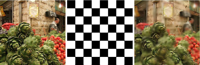
Figure 8: An example of using the extended convolution for adaptive smoothing. Given an image (left) and a transformation field (center) the extended convolution can adaptively smooth the image (right) so that darker points in the transformation field maintain feature detail while lighter points are blurred out.

To apply the extended convolution to image smoothing, we need to modify the output of the extended convolution so that the value at every point is defined as the weighted average of its neighbors. Treating the value $\bigl{(}\{H,\ {\mathfrak{T}}\}*F\bigr{)}(p)$ as the weighted sum of contributions from the neighbors of $p$, we can do this by dividing the value at $p$ by the total sum of weights. That is, if we denote by $\{1,\ {\mathfrak{T}}\}*F$ the extended convolution with a signal whose value is $1$ everywhere, the adaptively smoothed signal can be defined as:

$$\frac{\{H,\ {\mathfrak{T}}\}*F}{\{1,\ {\mathfrak{T}}\}*F}.$$ (13)

To localize the smoothing, we modify the signal. Specifically, using the fact that scaling the filter $F$ by ${\mathfrak{T}}(q)$ scales its integral by ${\mathfrak{T}}^{2}(q)$, we normalize the signal $H$, setting:

$$\tilde{H}(q)=\frac{H(q)}{\|{\mathfrak{T}}(q)\|^{2}}$$

so that the extended convolution $\{\tilde{H},\ {\mathfrak{T}}\}*F$ distributes the value $H(q)$ to its neighbors, using a unit-integral distribution. Note that this modification is necessary only when the transformation field ${\mathfrak{T}}$ includes scaling; it is not needed when ${\mathfrak{T}}$ consists of rotations.

As an example, Figure 9, left, shows the results of the extended convolution for the market stall signal and checkerboard transformation mask, without a division by $\{1,\ {\mathfrak{T}}\}*F$. Because the filters in the black regions in the mask have smaller variance, the corresponding regions in the image accumulate less contribution and are darker.

Dividing by $\{1,\ {\mathfrak{T}}\}*F$, we obtain Figure 9, right. The pixels now have the correct luminance, but because the filters used in the light portions are not normalized to have unit-integral, the adaptively smoothed image exhibits blur-bleeding across the mask boundaries. The correct result, with normalized $\tilde{H}$, is shown in Figure 8, right.

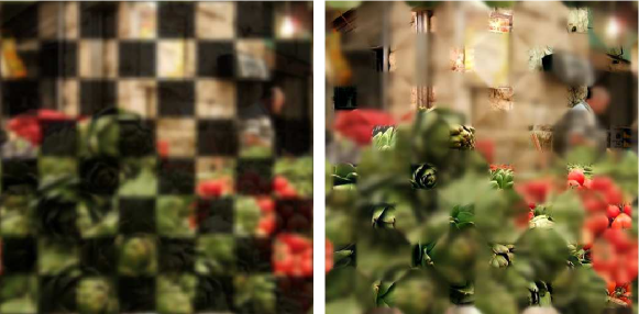
Figure 9: Left: If the value of a pixel is not normalized by the weighted average of its neighbors, the luminance is affected by the filter variance at each pixel. Right: Normalizing for filter variance, but failing to account for filter scale change, results in blur-bleeding across sharp edges in the transformation mask.

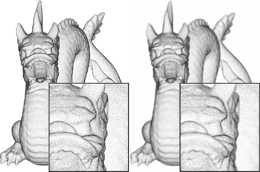
Figure 10: Left: A wire-frame visualization of a dragon model. Right: A simulation of depth-defocus obtained by using the depth values to set the scaling mask in performing adaptive smoothing on the wire-frame visualization.

An example of adaptive smoothing with a more complex scaling mask is shown in Figure 10. The image on the left shows a wire-frame visualization of a dragon model and the image on the right shows the results of adaptive smoothing applied to the visualization. For the scaling mask, we set:

$${\mathfrak{T}}(p)=|Z(p)-Z(p_{0})|$$

where $Z(p)$ is the value of the $z$-buffer at pixel $p$, and $p_{0}$ are the pixel coordinates of the center of the dragon’s left eye. For the filter, we used the indicator function of a disk, smoothed along the radial directions. Smoothing was necessary to ensure that undesirable ringing artifacts did not arise when we approximated the extended convolution by using only the first 64 frequencies. This visualization simulates the depth-defocus (e.g. [PC81, Dem04, ST04, KLO06]) resulting from imaging the dragon with a wide-aperture camera whose depth-of-field is set to the depth at the dragon’s left eye. Although the implementation does not take into account the depth-order of pixels, and hence does not provide a physically accurate simulation of the effects of depth-defocus, it generates convincing visualizations that can be used to draw the viewer’s eye to specific regions of interest.

The effectiveness of adaptive blurring is made possible by two properties: First, despite the band-limiting of the filter, adaptive blurring accurately reproduces fine detail, such as the single-pixel-width wire-frame lines in the left eye. Second, because the extended convolution is implemented as a scattering operation, it exhibits fewer of the edge-bleeding artifacts known to be difficult (e.g. [KLO06]) in “gathering” implementations.

As a further example of the effects achievable using adaptive filtering, we demonstrate the use of extended convolution with a rotational field to implement the Line Integral Convolution (LIC) technique for vector field visualization [CL93]. We apply the extended convolution of a long, narrow anisotropic Gaussian kernel to a random noise image, using the given vector field’s angle at each pixel to determine the rotation to apply to the kernel. The result is shown in Figure 11, center, while at right we show the result produced when the normalization in (13) is not performed. The same technique was used to produce Figure 1, center: the gradient of the source image was used to define the rotational field, and noise was added to the image before applying extended convolution.

#   

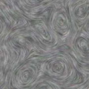
Figure 11: Line integral convolution for vector field visualization, implemented via extended convolution of a random noise image with the rotational field at left and a narrow anisotropic Gaussian filter. At right, we show the effects of not performing the normalization in (13) — while the result is not a correct convolution, it is nevertheless an effective visualization.

9 Function Steering in 3D

One of the contributions of our presentation is that it allows function steering to be generalized to higher dimensions. In this section, we discuss the limitations of using the classical formulation of function steering to adaptively rotate filters in 3D, and describe how such filtering can still be supported within our generalized, representation-theoretic framework.

As summarized in Section 4.4, classical steerable filtering with a filter $F$ is performed by using the functions $F_{0},\ldots,F_{K-1}$ as a steering basis, where $F_{j}$ is the rotation of the function $F$ by $j\pi/K$ and $K$ is the maximal angular frequency of the filter.

The efficiency of this implementation is based on three properties. (1) The space spanned by the $F_{j}$ is the $K$-dimensional space containing the orbit of $F$, so the functions $F_{j}$ can be used to steer the filter. (2) The number of rotations, $K$, is equal to the dimension of the space spanned by the orbit, so that the functions $F_{j}$ are the smallest set of functions required to steer $F$. And, (3) the filter is one of the basis functions, $F_{0}=F$, so that only $K$ of the functions $a_{i}F_{j}$ are non-zero, and hence an implementation of extended correlation only requires $K$ standard correlations.

What limits the extension of this approach to 3D function steering is that it is impossible to generically choose a set of $K$ rotations $R_{0},\ldots,R_{K-1}\in\hbox{SO}(3)$ such that $R_{0}$ is the identity and the functions $R_{0}(F),\ldots,R_{K}(F)$ are linearly independent. (See Appendix for more details.)

The inability to generalize classical steerable filtering to 3D has been observed before, and it has been suggested that an expansion into spherical harmonics might be used to accomplish this [FA91]. Our generalized approach provides the details, showing how to compute the extended correlation (resp. convolution) in a manner analogous to the one used for 2D rotations in Section 4.1. In this discussion, we will consider the spherical parameterization of the filter where we are assuming that $K=O(n^{1/3})$ is the maximal angular frequency, so that the dimensionality of each spherical function is $O(n^{2/3})$, and the radial resolution is $N=O(n^{1/3})$.

Filter Decomposition

We first decompose $F$ as the sum of functions with differing angular frequencies:

$$F=\sum_{l=0}^{K}\sum_{m=-l}^{l}F_{l}^{m}\qquad\hbox{with}\qquad F_{l}^{m}(r,\theta,\phi)=f_{l}^{m}\!(r)\,Y_{l}^{m}(\theta,\phi),$$

where the functions $Y_{l}^{m}$ are spherical harmonics of frequency $l$ and index $m$. This decomposition can be done by first expressing $F$ in spherical coordinates and then running the Fast Spherical Harmonic Transform [Sph98] at each radius to get the coefficients of the different frequency components. [$O(n+n\log^{2}n)$]

Standard Correlation

Next, we compute the standard correlations of the signal with the functions $f_{l}^{m^{\prime}}(r)Y_{l}^{m}(\theta,\phi)$:

$$G_{l}^{m,m^{\prime}}=H\star f_{l}^{m^{\prime}}F_{l}^{m}\qquad\forall\ l\in[0,K],\ m,m^{\prime}\in[-l,l].$$

This can be done by first evaluating the function $f_{l}^{m^{\prime}}F_{l}^{m}$ on a regular grid and then using the 3D Fast Fourier Transform to perform the correlation. [$O(n^{2}+n^{2}\log n)$]

Linear Combination

Finally, we take the linear combination of the correlation results:

$$\bigl{(}\{H,\ {\mathfrak{T}}\}\star F\bigr{)}(p)=\sum_{l=0}^{k}\,\sum_{m,m^{\prime}=-l}^{l}\overline{D_{m,m^{\prime}}^{l}\bigl{(}{\mathfrak{T}}(p)\bigr{)}}\,G_{l}^{m,m^{\prime}}(p),$$

where $D_{m,m^{\prime}}^{l}:\hbox{SO}(3)\rightarrow{\mathbb{C}}$ are the Wigner-D functions, giving the coefficient of the $(l,m^{\prime})$-th spherical harmonic within a rotation of the $(l,m)$-th spherical harmonic. [$O(n^{2})$]

Thus, our method provides a way for steering 3D functions, sampled on a regular grid with $n$ voxels, in time complexity $O(n^{2}\log n)$. If, as in the 2D case, we assume that the angular frequency of the filter is much smaller than the resolution of the voxel grid, $K\ll N$, the complexity becomes $O(nK^{3}\log n)$.

10 Conclusion

We have presented a novel method for extending the convolution and correlation operations, allowing for the efficient implementation of adaptive filtering. We have presented a general description of the approach, using principles from representation theory to guide the development of an efficient algorithm, and we discussed specific applications of the new operations to challenges in pattern matching and image processing.

In the future, we would like to apply extended convolutions using transformation fields consisting of both rotations and isotropic scales. We believe that this type of implementation opens the possibility for performing local shape-based matching over conformal parameterizations.

Defining Optimal Filters

Given an image $I$ and associated frame field ${\mathfrak{T}}$ and signal $H$, we seek a filter $F$, supported within a disk of radius of $\varepsilon$, whose extended convolution with the image is maximized (up to scale) at a point $q_{0}$.

Expanding the expression for the evaluation of the extended convolution at $q_{0}$, using the fact that evaluation at a point can be expressed by integrating against a delta function ($\delta$) at that point, and switching the order of integration, gives

$$\left(\{H,\ {\mathfrak{T}}\}*F\right)(q_{0})$$

$$=\int H(q)\ F\left({\mathfrak{T}}^{-1}(q)\cdot(q_{0}-q)\right)\ dq$$

$$=\int H(q)\ \left(\int F(p)\ \delta\left(p-{\mathfrak{T}}^{-1}(q)\cdot(q_{0}-q)\right)\ dp\right)\ dq$$

$$=\int F(p)\ \left(\int H(q)\ \delta\left(p-{\mathfrak{T}}^{-1}(q)\cdot(q_{0}-q)\right)\ dq\right)\ dp$$

$$=\int F(p)\ \left(\int H(q)\ \rho_{{\mathfrak{T}}^{-1}(q)\cdot(q_{0}-q)}\left(\ \delta(p)\ \right)\ dq\right)\ dp.$$

Thus, the filter $F$ supported within a disk of radius $\varepsilon$ that, up to scale, maximizes the response of the extended convolution at $q_{0}$, is

$$F =\int_{\|q_{0}-q\|\leq\varepsilon}H(q))\ \rho_{{\mathfrak{T}}^{-1}(q)\cdot(q_{0}-q)}\left(\delta\right)\ dq$$

$$=\int_{\|q\|\leq\varepsilon}H(q_{0}+q)\ \rho_{-{\mathfrak{T}}^{-1}(q_{0}+q)\cdot(q)}\left(\delta\right)\ dq.$$ (14)

Function Steering in 3D

To implement three-dimensional function steering with functions whose angular frequency is bounded by $K$, we would need to choose $N=(K+1)^{2}$ rotations $R_{0},\ldots,R_{N-1}\in\hbox{SO}(3)$ such that $R_{0}$ is the identity and the rotation of any (band-limited) filter $F$ could be expressed as the linear combination of the rotations of $F$:

$$R(F)=\sum_{j=0}^{N-1}\alpha_{j}(R)R_{j}F$$

Here, $\alpha_{j}:\hbox{SO}(3)\rightarrow{\mathbb{C}}$ is the function giving the coefficients of the $j$-th function and $\sum_{j=0}^{K}(2j+1)=(K+1)^{2}$ is the dimension of the space of spherical functions whose angular frequency is bounded by $K$.

The problem is that such a choice of rotations and hence the definition of the coefficient functions $\alpha_{j}$, needs to depend on the filter $F$. To see this, we show that for any choice of rotations, $R_{1},\ldots,R_{N-1}$, we can always find a spherical function $F$ whose orbit under the group of rotations spans an $N$-dimensional space but has the property that the functions $R_{0}F,\ldots,F_{N-1}F$ are linearly dependent, and cannot span the same space.

Consider the rotations $R_{0}$ and $R_{1}$, the former is the identity map, and the latter must be a rotation about some axis, which (without loss of generality) we assume to be the $y$-axis. Consequently, any function that is axially symmetric about the $y$-axis must be fixed by both rotations. In particular, this implies that any linear combination of the zonal harmonics has to be fixed. On the one hand, this implies that functions $\{R_{0}F,\ldots,R_{N-1}F\}$ span a space whose dimension is no larger than $N-1$ (since $R_{0}F=R_{1}F$) on the other hand, we know that if the coefficients of all the zonal harmonics are non-zero, the orbit of $F$ under the action of the rotation group must span an $N$-dimensional space. Thus, it is impossible to express all rotations of $F$ using linear combinations of $\{R_{0}F,\ldots,R_{N-1}F\}$.

Note that while this precludes the extension of classical steerable filtering to the steering of arbitrary functions in 3D, a more restricted version can still be implemented if the space of filters is constrained. Such a restriction is described in the work of Freeman and Adelson, where they discuss the possibility of filtering with functions that are rotationally symmetric about the $y$-axis. Since the only rotations fixing such filters are rotations about the $y$-axis, this subspace of functions may be steered if the rotations $R_{1},\ldots,R_{N-1}$ do not fix the $y$-axis.

References

- [All77] Allen J.: Short term spectral analysis, synthesis and modification by discrete Fourier transform. In IEEE Trans. Acoustics, Speech, and Signal Processing (1977), vol. 25, pp. 235–238.
- [Bal81] Ballard D.: Generalizing the hough transform to detect arbitrary shapes. Pattern Recognition 13 (1981), 111–122.
- [Bra00] Bradski G.: The OpenCV Library. Dr. Dobb’s Journal of Software Tools (2000).
- [BTFN∗08] Brown B., Toler-Franklin C., Nehab D., Burns M., Dobkin D., Vlachopoulos A., Doumas C., Rusinkiewicz S., Weyrich T.: A system for high-volume acquisition and matching of fresco fragments: Reassembling Theran wall paintings. ACM Transactions on Graphics (Proc. SIGGRAPH) 27, 3 (Aug 2008).
- [CK16] Chirikjian G. S., Kyatkin A. B.: Harmonic Analysis for Engineers and Applied Scientists: Updated and Expanded Edition. Courier Dover Publications, 2016.
- [CL93] Cabral B., Leedom L.: Imaging vector fields using line integral convolution. In Proc. SIGGRAPH (1993).
- [CT65] Cooley J., Tukey J.: An algorithm for the machine calculation of complex Fourier series. Math. Comput. 19 (1965), 297–301.
- [Dem04] Demers J.: Depth of Field: A Survey of Techniques. Addison-Wesley Professional, 2004, ch. 23, pp. 375–390.
- [FA91] Freeman W., Adelson E.: The design and use of steerable filters. IEEE Trans. Pattern Analysis and Machine Intelligence 13, 9 (1991), 891–906.
- [FJ05] Frigo M., Johnson S.: The design and implementation of FFTW3. Proceedings of the IEEE 93, 2 (2005), 216–231.
- [GBS∗16] Guo Y., Bennamoun M., Sohel F., Lu M., Wan J., Kwok N. M.: A comprehensive performance evaluation of 3d local feature descriptors. International Journal of Computer Vision 116 (2016), 66–89.
- [HFG∗06] Huang Q.-X., Flöry S., Gelfand N., Hofer M., Pottmann H.: Reassembling fractured objects by geometric matching. ACM Trans. Graphics 25 (2006), 569–578.
- [HLS18] He K., Lu Y., Sclaroff S.: Local descriptors optimized for average precision. In Computer Vision and Pattern Recognition (2018), pp. 596–605.
- [Ior01] Iorio R.: Fourier Analysis and Partial Differential Equations. Cambridge University Press, 2001.
- [JMM∗20] Jin Y., Mishkin D., Mishchuk A., Matas J., Fua P., Yi K. M., Trulls E.: Image matching across wide baselines: From paper to practice. arXiv preprint arXiv:2003.01587 (2020).
- [KC99a] Kyatkin A. B., Chirikjian G. S.: Computation of robot configuration and workspaces via the fourier transform on the discrete-motion group. The International Journal of Robotics Research 18, 6 (1999), 601–615.
- [KC99b] Kyatkin A. B., Chirikjian G. S.: Pattern matching as a correlation on the discrete motion group. Computer vision and image understanding 74, 1 (1999), 22–35.
- [KFR04] Kazhdan M., Funkhouser T., Rusinkiewicz S.: Symmetry descriptors and 3D shape matching. In Eurographics Symposium on Geometry Processing 2004 (2004), vol. 2, pp. 116–125.
- [KJM05] Kumar V., Juday R., Mahalanobis A.: Correlation Pattern Recognition. Cambridge University Press, 2005.
- [KLO06] Kass M., Lefohn A., Owens J.: Interactive Depth of Field Using Simulated Diffusion on a GPU. Tech. Rep. 06-01, Pixar Animation Studios, January 2006.
- [KM90] Kass M., Miller G.: Stable fluid dynamics for computer graphics. In Proceedings of Computer Graphics (SIGGRAPH ’90) (1990), vol. 24, pp. 49–57.
- [KPS17] Karami E., Prasad S., Shehata M.: Image matching using SIFT, SURF, BRIEF and ORB: performance comparison for distorted images. arXiv preprint arXiv:1710.02726 (2017).
- [KS01] Kak A., Slaney M.: Principles of Computerized Tomographic Imaging. Society of Industrial and Applied Mathematics, 2001.
- [KS04] Ke Y., Sukthankar R.: PCA-SIFT: A more distinctive representation for local image descriptors. In Computer Vision and Pattern Recognition (2004), vol. 2, IEEE, pp. 506–513.
- [KS06] Keller Y., Shkolnisky Y.: A signal processing approach to symmetry detection. IEEE Trans. Image Processing 15 (2006), 2198–2207.
- [KWG83] Knutsson H., Wilson R., Granlund G.: Anisotropic nonstationary image estimation and its applications: Part 1-restoration of noisy images. IEEE Transactions on Communications 31 (1983), 388–397.
- [Low04] Lowe D. G.: Distinctive image features from scale-invariant keypoints. International Journal of Computer Vision 60 (2004), 91–110.
- [LS02] Leitão H. C. G., Stolfi J.: A multiscale method for the reassembly of two-dimensional fragmented objects. IEEE Trans. Pattern Analysis and Machine Intelligence 24, 9 (2002), 1239–1251.
- [LSZ∗18] Luo Z., Shen T., Zhou L., Zhu S., Zhang R., Yao Y., Fang T., Quan L.: Geodesc: Learning local descriptors by integrating geometry constraints. In European Conference on Computer Vision. (2018), pp. 168–183.
- [MK03] McBride J., Kimia B.: Archaeological fragment reconstruction using curve-matching. In Proc. Computer Vision and Pattern Recognition Workshop (2003), vol. 1.
- [MMRM17] Mishchuk A., Mishkin D., Radenovic F., Matas J.: Working hard to know your neighbor’s margins: Local descriptor learning loss. In Advances in Neural Information Processing Systems (2017), pp. 4826–4837.
- [Moo77] Moorer J.: Signal processing aspects of computer music: A survey. In Proceedings of the IEEE (1977), vol. 65, pp. 1108–1137.
- [MS05] Mikolajczyk K., Schmid C.: A performance evaluation of local descriptors. Transactions on Pattern Analysis and Machine Intelligence 27 (2005), 1615–1630.
- [Nat01] Natterer F.: The Mathematics of Computerized Tomography. Society for Industrial and Applied Mathematics, Philadelphia, Pennsylvania, 2001.
- [PC81] Potmesil M., Chakravarty I.: A lens and aperture camera model for synthetic image generation. In Computer Graphics (Proceedings of SIGGRAPH 81) (1981), vol. 15, pp. 297–305.
- [PM90] Perona P., Malik J.: Scale-space and edge detection using anisotropic diffusion. Transactions on Pattern Analysis and Machine Intelligence 12 (1990), 629–639.
- [SBS06] Schall O., Belyaev A., Seidel H.: Adaptive Fourier-based surface reconstruction. In Geometric Modeling and Processing (2006), vol. 4, pp. 34–44.
- [Ser77] Serre J.: Linear Representations of Finite Groups. Springer-Verlag, New York, 1977.
- [SF96] Simoncelli E., Farid H.: Steerable wedge filters for local orientation analysis. IEEE Transactions on Image Processing 5 (1996), 1377–1382.
- [SHSP17] Schonberger J. L., Hardmeier H., Sattler T., Pollefeys M.: Comparative evaluation of hand-crafted and learned local features. In Computer Vision and Pattern Recognition (2017), pp. 1482–1491.
- [SMKF04] Shilane P., Min P., Kazhdan M., Funkhouser T.: The Princeton shape benchmark. In Proceedings Shape Modeling Applications (2004), pp. 167–178.
- [Sph98] SpharmonicKit 2.5: http://www.cs.dartmouth.edu/~geelong/sphere/, 1998.
- [ST04] Scheuermann T., Tatarchuk N.: Improved depth-of-field rendering. Charles River Media, 2004, ch. 4.4, pp. 363–377.
- [Sta01] Stam J.: A simple fluid solver based on the FFT. Journal of Graphics Tools 6 (2001), 43–52.
- [THO99] Teo P., Hel-Or Y.: Design of multi-parameter steerable functions using cascade basis reduction. IEEE Transactions on Pattern Analysis and Machine Intelligence 21 (1999), 552–556.
- [TM98] Tomasi C., Manduchi R.: Bilateral filtering for gray and color images. In Proceedings of the Sixth International Conference on Computer Vision ’98 (1998), pp. 839–846.
- [TS18] Tareen S. A. K., Saleem Z.: A comparative analysis of SIFT, SURF, KAZE, AKAZE, ORB, and BRISK. In 2018 International Conference on Computing, Mathematics and Engineering Technologies (2018), pp. 1–10.
- [Wal91] Wallace G.: The JPEG still picture compression standard. Communications of the ACM 34 (1991), 30–44.
- [Wei97] Weickert J.: A review of nonlinear diffusion filtering. In Proceedings of the First International Conference on Scale-Space Theory in Computer Vision (1997), pp. 1–28.
- [Wei06] Weiss B.: Fast median and bilateral filtering. ACM Trans. Graphics 25 (2006), 519–526.
- [ZFR19] Zhang L., Finkelstein A., Rusinkiewicz S.: High-precision localization using ground texture. In International Conference on Robotics and Automation (2019).
- [ZR19] Zhang L., Rusinkiewicz S.: Learning local descriptors with a CDF-based dynamic soft margin. In International Conference on Computer Vision (2019).