Scintillation can explain the spectral structure of the bright radio burst from SGR 1935+2154

Abstract

The discovery of a fast radio burst (FRB) associated with a magnetar in the Milky Way by the Canadian Hydrogen Intensity Mapping Experiment FRB collaboration (CHIME/FRB) and the Survey for Transient Astronomical Radio Emission 2 (STARE2) has provided an unprecedented opportunity to refine FRB emission models. The burst discovered by CHIME/FRB shows two components with different spectra. We explore interstellar scintillation as the origin for this variation in spectral structure. Modeling a weak scattering screen in the supernova remnant associated with the magnetar, we find that a superluminal apparent transverse velocity of the emission region of $>9.5\,c$ is needed to explain the spectral variation. Alternatively, the two components could have originated from independent emission regions spaced by $>8.3\times 10^{4}$ km. These scenarios may arise in “far-away” models where the emission originates from well beyond the magnetosphere of the magnetar (for example through a synchrotron-maser mechanism set up by an ultra-relativistic radiative shock), but not in “close-in” models of emission from within the magnetosphere. If further radio observations of the magnetar confirm scintillation as the source for the observed variation in spectral structure, this scattering model thus constrains the location of the emission region.

1 Introduction

On the 28th of April, 2020, the fast radio burst project of the Canadian Hydrogen Intensity Mapping Experiment (CHIME/FRB) detected a bright two-component millisecond-timescale radio burst in the direction of the galactic magnetar SGR 1935+2154 (The CHIME/FRB Collaboration et al., 2020). The coincidence of this burst with a one-second-long hard X-ray burst (Mereghetti et al., 2020; Ridnaia et al., 2020; Tavani et al., 2020; Zhang et al., 2020b) provides an unambiguous association of the CHIME/FRB radio detection with SGR 1935+2154, and stringently constrains models for the radio emission (Margalit et al., 2020a; Lu et al., 2020; Yuan et al., 2020; Lyutikov & Popov, 2020). In addition to the CHIME/FRB-detected burst in the 400–800 MHz band, a single-component burst was detected by the STARE2 instrument at 1281–1468 MHz (Bochenek et al., 2020), likely associated with the latter component of the CHIME/FRB detection. A $10^{7}$ times fainter burst was detected two days later by the FAST telescope in the 1.4 GHz band (Zhang et al., 2020a), and Burgay et al. (2020) later reported a tentative detection of persistent faint pulsed emission at 408 MHz.

The bright radio burst from SGR 1935+2154 exhibited a larger (by a few orders of magnitude) isotropic-equivalent energy than any radio burst previously observed from within the Milky Way. The fluences of $700^{+700}_{-350}$ kJy ms and $1.5\pm 0.3$ MJy ms measured by CHIME/FRB and STARE2 respectively, combined with a distance estimate of $\sim 10$ kpc to SGR 1935+2154, are consistent with a modest low-energy extrapolation of the extragalactic FRB population (Bochenek et al., 2020; The CHIME/FRB Collaboration et al., 2020). This suggests that magnetars like SGR 1935+2154 are viable sources of FRBs at extragalactic distances. In interpreting our results in this paper, we focus on two classes of emission models that were developed for extragalactic FRBs, but have been applied to the burst from SGR 1935+2154. “Close-in” models (Lyutikov & Popov, 2020; Lu et al., 2020) posit that the radio emission is generated at heights of $\lesssim 100\,r_{\mathrm{NS}}$, where $r_{\mathrm{NS}}\sim 10$ km is the neutron-star (NS) radius. A possible mechanism is the decay, at $\sim 20\,r_{\mathrm{NS}}$, of Alfvén waves launched from the magnetar surface by the same disturbance that generates the hard X-ray emission (Lu et al., 2020). On the other hand, “far-away” models require that magnetar bursts cause the ejection of a portion of the magnetosphere (known as a plasmoid) at relativistic speeds into the surrounding medium (Margalit et al., 2020a; Yuan et al., 2020). The plasmoid will shock the highly magnetized surrounding medium at distances of $10^{11}$ cm (Margalit et al., 2020a) to $10^{13}$ cm (Yuan et al., 2020) with Lorentz factors of a few tens (Margalit et al., 2020a) to a few hundreds (Yuan et al., 2020) depending on the composition of the medium. The shock will primarily dissipate radiatively in the high-energy portion of the electromagnetic spectrum, but will also be accompanied by prompt radio emission through the synchrotron maser mechanism. The position and velocity of the radio-emitting region are thus important discriminants between different models for the bright radio burst from SGR 1935+2154.

The two components in the burst detected by CHIME/FRB have different spectra. The earlier burst is brightest in the bottom of the observing band (400–600 MHz) while the later burst is faint at frequencies below $\sim 500$ MHz, but otherwise occupies the majority of the 400–800 MHz band (see Fig. 1 of The CHIME/FRB Collaboration et al. (2020).) Both components appear to be temporally broadened by the effects of multi-path propagation through the Milky Way interstellar medium (ISM), commonly referred to as “scattering”. The CHIME/FRB Collaboration et al. (2020) fit a characteristic scattering timescale of $0.759\pm 0.008$ ms simultaneously to the two components at 600 MHz. Scattering was also tentatively observed in the higher-frequency burst detected by STARE2 (Bochenek et al., 2020).

Spectral differences in emission components have been seen from extragalactic repeating FRBs (Hessels et al., 2019; CHIME/FRB Collaboration et al., 2019a, b); however, in these repeating FRBs the peak frequencies of components that arrive later are invariably lower, not higher. The origin of this characteristic repeating-FRB spectral structure remains unknown. Cordes et al. (2017) suggests it may arise from lensing within the host galaxy of the FRB source (for example, within a wind nebula or SNR associated with the FRB source, or an HII region within the galaxy), while Metzger et al. (2019) and Margalit et al. (2020b) explain this change in peak frequency within their synchrotron maser model as a deceleration of the shock front. This makes it difficult for the “far-away” emission models to explain the differences in the spectra of the two components of the radio burst from SGR 1935+2154 (Lu et al., 2020). The sharp cutoffs in the spectra of both bursts are difficult to explain without contrived discontinuities in the pre-shock medium; see the Appendix of Lu et al. (2020) for further details.

In this letter, we posit that the observed variation in spectral structure between the two components of the CHIME/FRB-detected burst is due to interstellar scintillation. In the picture we present in Section 2, two separate scattering screens intervene along the line-of-sight to SGR 1935+2154: one responsible of the observed temporal broadening of the burst and one responsible for the observed spectral structure. The differences in the spectra of the two bursts allow us to place a lower limit on the separation between the sources of the two bursts, which can be interpreted as either motion of the emission region or a spatial separation between two independent emission regions. We discuss the implications of this limit on models for FRB-like emission from magnetars in Section 3, and discuss ways in which our picture could be further tested in Section 4.

2 A two-screen model for the spectral properties of the two-component SGR 1935+2154 radio burst detected by CHIME/FRB

Two-screen scattering models have recently gained traction in the study of propagation effects for extragalactic FRBs (Masui et al., 2015; Ravi et al., 2016; Farah et al., 2018; CHIME/FRB Collaboration et al., 2019c; Macquart et al., 2019; Day et al., 2020); typically these are motivated by scattering inconsistent with expectations from the Milky Way or by incongruous temporal scatter-broadening timescales and scintillation bandwidths. In this letter, “scintillation” refers specifically to spectral modulations caused by the coherent combination of radiation propagating along different paths, and “scattering” refers to the general occurrence of multi-path propagation, which may manifest as scintillation or temporal broadening of pulses, among several phenomena (Rickett, 1990). For extragalactic FRBs, scintillation is typically associated with the effects of diffraction within the Milky Way, while the temporal broadening of the burst is attributed to additional scattering material associated with the circumburst medium, the ISM of the host galaxy or the halos of intervening galaxies.

Multiple scattering screens are also inferred in the Milky Way from pulsar scattering observations (e.g. Putney & Stinebring, 2006). In some cases, such as scattering towards the Galactic Center (in observations of both Sgr A* and the Galactic-Center magnetar SGR J1745-2900), one of the scattering screens is very close to the source of emission (Dexter et al., 2017). Similar evidence for scattering near the source is seen towards the Crab pulsar, PSR B0531+21 (e.g. Cordes et al., 2004; Main & van Kerkwijk, 2018; Driessen et al., 2019). Scintillation with characteristic bandwidths of 1 MHz at 1.66 GHz (Main & van Kerkwijk, 2018) and 2.3 MHz at 2.33 GHz (Cordes et al., 2004) is associated with scattering in the Crab nebula due to the rapid decorrelation timescales of the scintillation pattern.

Below, we explore the viability of a similar two-screen model for SGR 1935+2154, in which the spectral structure in the CHIME/FRB-detected burst is due to scintillation with an estimated scintillation half-width half-maximum bandwidth of 100 MHz at 600 MHz. This corresponds to a bandwidth of 770 MHz at 1 GHz, consistent with the combined detection of the second component by CHIME/FRB and STARE2. The observing parameters we will use are summarized in Table 1. The difference in the observed scintillation properties between the two components of the burst necessitates that the scintillation pattern upon the Earth has moved by at least the spatial scale of the scintle in the 28.97 ms separating the two components. We use this constraint on the velocity of the scintillation pattern to constrain the velocity of the emission region (if the same emission region is responsible for both components) or separations of two emission regions (if each component arose from a different region).

Table 1: Parameters measured or assumed for the CHIME/FRB bursts from SGR 1935+2154 and used throughout this work.

Parameter	Value	Description
Measured Parameters
$\nu_{\mathrm{ref}}$	600 MHz	Reference frequency for scattering and scintillation parameters
$\Delta t$	28.97 ms	Temporal separation between the two components
$\tau_{\mathrm{scat}}$	$0.759\pm 0.008$ ms	Scattering timescale fit by The CHIME/FRB Collaboration et al. (2020)
$\Delta\nu_{\mathrm{scint}}$	100 MHz	Scintillation (HWHM) bandwidth estimated from the dynamic spectra of the CHIME/FRB-detected radio burst
Derived Parameters
$\tau_{\mathrm{scint}}$	1.5 ns	Scattering timescale corresponding to $\Delta\nu_{\mathrm{scint}}$
$\Delta\nu_{\mathrm{scat}}$	200 Hz	Scintillation bandwidth corresponding to $\tau_{\mathrm{scat}}$
Fiducial Parameters
$d_{\mathrm{src}}$	10 kpc	Fiducial distance to SGR 1935+2154
$d_{\mathrm{scat}}$	5 kpc	Distance to the scattering screen responsible for temporal-broadening
$d_{\mathrm{scint}}$	9.984 kpc	Distance to the scattering screen responsible for scintillation
$s_{\mathrm{scat}}$	0.5	$s_{\mathrm{scat}}=1-d_{\mathrm{scat}}/d_{\mathrm{src}}$
$s_{\mathrm{scint}}$	$1.6\times 10^{-3}$	$s_{\mathrm{scint}}=1-d_{\mathrm{scint}}/d_{\mathrm{src}}$
$C_{1}$	0.957	Equation (2)
Other Parameters
$l_{d}$		$1/e$ half-width of the spatial scintillation pattern
$V_{\mathrm{src,app}}$		Apparent transverse velocity of the emission region
$V_{\mathrm{ISS}}$		Velocity of the scintillation pattern on the observer plane
$\Delta t_{\mathrm{scint}}$		Decoherence timescale of the scintillation pattern

We start by considering the locales of the two scattering regions. The NE2001 model (Cordes & Lazio, 2002, 2003) predicts a scattering timescale of 0.048 ms at 1 GHz, which scales to 0.37 ms at 600 MHz (assuming a timescale $\tau\propto\nu^{-4}$), off only by a factor of two from the measured scattering timescale. This suggests that the temporal broadening arises in the ISM as modeled in NE2001. In contrast, a scintillation bandwidth of 100 MHz corresponds to a scattering timescale of 1.5 ns, much smaller than (and therefore easily concealed by) the 0.759 ms timescale. Thus, we will consider below a picture in which the temporal broadening originates in the ISM while the scintillation is dominated by scattering closer to SGR 1935+2154. We consider the reverse scenario in Appendix A.

The distance to SGR 1935+2154 remains uncertain, with recent measurements of the distance to the associated supernova remnant SNR G57.2+0.8 including $6.6\pm 0.7$ kpc (Zhou et al., 2020) and $12.5\pm 1.5$ kpc (Kothes et al., 2018). We will adopt a fiducial distance of $d_{\mathrm{src}}=10$ kpc. Screens halfway between the observer and the source contribute most significantly to temporal broadening, so we will use a fiducial distance to the screen responsible for temporal broadening of $d_{\mathrm{scat}}=\frac{1}{2}d_{\mathrm{src}}$. Finally, the SNR associated with SGR 1935+2154 has an angular radius of 5.5 arcminutes. As this SNR is a possible location of scattering near the host, we will adopt a fiducial fractional distance between SGR 1935+2154 and the screen responsible for scintillation of $s_{\mathrm{scint}}=1-\frac{d_{\mathrm{scint}}}{d_{\mathrm{src}}}=1.6\times 10^{-3}$. Kothes et al. (2018) also identify a second arc-like feature in the GMRT 150-MHz survey radio map (Intema et al., 2017), with an approximate angular radius of 3.6 arcminutes (estimated from their Fig. 2). This feature, which, as Kothes et al. (2018) consider, could be a pulsar wind nebula (PWN)-like feature produced by the magnetar, is another possible location for scattering (with $s_{\mathrm{scint}}=1.0\times 10^{-3}$).

The $1/e$ half-width of the scintillation pattern projected on the observer plane, assuming isotropic scattering in a thin screen a distance $d_{\mathrm{lens}}$ from the observer, is given by (Cordes & Rickett, 1998)

$$l_{d} =\frac{1}{\nu_{\mathrm{ref}}}\left(\frac{c\Delta\nu_{d}}{2\pi C_{1}}\frac{d_{\mathrm{src}}d_{\mathrm{lens}}}{d_{\mathrm{src}}-d_{\mathrm{lens}}}\right)^{1/2}\;,$$ (1)

where $\nu_{\mathrm{ref}}$ is the reference frequency, $\Delta\nu_{d}$ is the half-width half-max scintillation bandwidth, and $C_{1}$ is a factor that depends on the spectrum of density fluctuations and the distribution of the scattering material, defined by the relationship between the scintillation bandwidth and the mean delay:

$$2\pi\Delta\nu_{d}\tau_{d}=C_{1}\;.$$ (2)

We will use $C_{1}=0.957$ for a Kolmogorov phase structure function of the radiation scattered by a thin screen (Cordes & Rickett, 1998). Adopting our fiducial values, Equation (1) can be written as

$$l_{d} =5.2\times 10^{7}\,\mathrm{km}\left(\frac{\nu_{\mathrm{ref}}}{600\,\mathrm{MHz}}\right)^{-1}\left(\frac{\Delta\nu_{d}}{100\,\mathrm{MHz}}\right)^{1/2}\left(\frac{d_{\mathrm{src}}}{10\,\mathrm{kpc}}\right)^{1/2}\left(\frac{(1-s)s^{-1}}{624}\right)^{1/2}\;,$$ (3)

where $s=1-\frac{d_{\mathrm{lens}}}{d_{\mathrm{src}}}$. For $s=1.6\times 10^{-3}$, the spatial size of the scintillation pattern is $5.2\times 10^{7}$ km, many times the size of the Earth.

The differing spectra observed between the two components of the burst necessitates that, if this spectral structure is due to scintillation, the scintillation pattern has moved by at least $l_{d}$ within the temporal separation of the two components, $\Delta t=28.97$ ms, or

$$V_{\mathrm{ISS}}\geq\frac{l_{d}}{\Delta t}\;,$$ (4)

where $V_{\mathrm{ISS}}$ is the velocity of the scintillation pattern in the plane of the observer. When the scattering screen is very close to the source, this motion is related to the apparent transverse motion of the source by

$$V_{\mathrm{src,app}}=\frac{s}{1-s}V_{\mathrm{ISS}}\;,$$ (5)

allowing us to constrain the apparent transverse motion of the source to be

$$V_{\mathrm{src,app}}\geq\frac{1}{\nu_{\mathrm{ref}}\Delta t}\left(\frac{c\Delta\nu_{d}d_{\mathrm{src}}}{2\pi C_{1}}\frac{s}{1-s}\right)^{1/2}\;.$$ (6)

In terms of our fiducial parameters:

$$V_{\mathrm{src,app}}\geq 9.5\,c\left(\frac{\nu_{\mathrm{ref}}}{600\,\mathrm{MHz}}\right)^{-1}\left(\frac{\Delta t}{28.97\,\mathrm{ms}}\right)^{-1}\left(\frac{\Delta\nu_{d}}{100\,\mathrm{MHz}}\right)^{1/2}\left(\frac{d_{\mathrm{src}}}{10\,\mathrm{kpc}}\right)^{1/2}\left(\frac{(1-s)s^{-1}}{624}\right)^{-1/2}\;.$$ (7)

For $s=1.6\times 10^{-3}$, $V_{\mathrm{src,app}}\geq 9.5\,c$. We can interpret this either as superluminal motion of the emission region, or as a spatial separation of $V_{\mathrm{src,app}}\,\Delta t\geq 8.3\times 10^{4}$ km between two emission regions. The scintillation bandwidth we use is uncertain, likely to a factor of $\sim 2$. As we see from Equation (7), our estimate for the apparent transverse velocity of the source depends on the square root of the scintillation bandwidth and therefore, for our fiducial distances to the source and scintillation-dominating screen, our inferred velocity of the source is in the range of $6.7-13.5\,c$ or transverse separation of $5.9-11.7\times 10^{4}$ km. As these variations are not sufficiently significant to affect the conclusions of this work, we consider only the fiducial value of 100 MHz going forward.

The diffractive scale, $r_{\mathrm{diff}}$, the typical spatial scale of density fluctuations at the screen, can be calculated for a scattering screen from a measurement of the scintillation bandwidth $\Delta\nu_{d}$ and the assumed distributions of scattering material and density fluctuations. For isotropic Kolmogorov turbulence in a thin screen distance $d_{\mathrm{lens}}$, the diffractive scale is given by (Macquart & Koay, 2013):

$$r_{\mathrm{diff}} =\frac{1}{\nu_{\mathrm{ref}}}\left(\frac{\Delta\nu_{d}\,d_{\mathrm{src}}\,c}{2\pi C_{1}}\,s(1-s)\right)^{1/2}$$ (8)

$$=8.3\times 10^{9}\,\mathrm{cm}\left(\frac{\nu_{\mathrm{ref}}}{600\,\mathrm{MHz}}\right)^{-1}\left(\frac{\Delta\nu_{d}}{100\,\mathrm{MHz}}\right)^{1/2}\left(\frac{d_{\mathrm{src}}}{10\,\mathrm{kpc}}\right)^{1/2}\left(\frac{s(1-s)}{1.6\times 10^{-3}}\right)^{1/2}\;.$$ (9)

For $s=1.6\times 10^{-3}$, $r_{\mathrm{diff}}=8.3\times 10^{9}$ cm, larger than the typical inner scale $l_{\mathrm{inner}}=100$ km in the ISM (Spangler & Gwinn, 1990).

When $r_{\mathrm{diff}}>l_{\mathrm{inner}}$, the scattering measure (SM) is related to the diffractive scale by (Macquart & Koay, 2013)

$$\mathrm{SM} =\left(\frac{1}{2}r_{\mathrm{diff}}\right)^{-5/3}\frac{3\nu_{\mathrm{ref}}^{2}}{11\pi c^{2}r_{e}^{2}}\frac{\Gamma(\frac{11}{6})}{\Gamma(\frac{-11}{6})}$$ (10)

$$=7.4\times 10^{-5}\,\mathrm{kpc}\,\mathrm{cm}^{-20/3}\left(\frac{\nu_{\mathrm{ref}}}{600\,\mathrm{MHz}}\right)^{11/3}\left(\frac{\Delta\nu_{d}}{100\,\mathrm{MHz}}\right)^{-5/6}\left(\frac{d_{\mathrm{src}}}{10\,\mathrm{kpc}}\right)^{-5/6}\left(\frac{s(1-s)}{1.6\times 10^{-3}}\right)^{-5/6}\;,$$ (11)

where $r_{e}$ is the classical electron radius and $\Gamma(.)$ is the Gamma function. For $s_{\mathrm{scint}}=1.6\times 10^{-3}$, $\mathrm{SM}=7.4\times 10^{-5}$ kpc m^-20/3. This is low compared to typical measurements of the SM in the ISM using pulsar scattering, which vary between $\sim 0.01-100$ kpc m^-20/3 (Bhat et al., 2004). However, most studies of pulsar scattering focus on scattering timescales measured within a narrow bandwidth, and thus select against weakly scattering material. This is compounded by the fact that few instruments are able to probe scintillation bandwidths that cover such a large fraction ($1/6^{\mathrm{th}}$, in this case) of the central observing frequency. Ongoing and future wide-band pulsar studies (e.g. with the MWA (Kirsten et al., 2019), LOFAR (Stappers et al., 2011), MeerTime (Bailes et al., 2018), CHIME/Pulsar (Ng, 2018), and pulsar timing with the Parkes Ultra-Wideband (UWL) receiver (Hobbs et al., 2020)) will provide more insight into the prevalence of weakly-scattering material in the Milky Way.

If the scattering material is in fact closer to the source, the derived SM of the material decreases while the lower limit on the speed of emission region (or on the separation between two emission regions) is relaxed, as shown in Fig. 1. As the distance to SGR 1935+2154 is uncertain to $<50\%$, it has a much less significant impact on the inferred properties of the scattering material and the emission mechanism than the location of the scattering material.

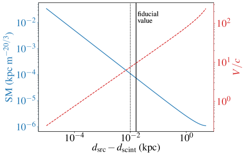
Figure 1: Dependence of scattering measure (SM, solid blue line, left-hand axis) and the derived lower limit on the velocity of the emission region ($V$, in units of $c$, dashed red line, right-hand axis) on the distance between SGR 1935+2154 and the scattering material responsible for scintillation. The velocity can also be interpreted as a separation between two emission regions, each responsible for one of the observed components of the burst. With a separation of 28.97 ms between the components, $V/c=1$ corresponds to a separation of 8700 km. The fiducial separation between the screen and source of 16 pc, for which the screen is associated with the SNR G57.2+0.8, is indicated with the solid black line, while the separation of 10 pc corresponding to scattering in the putative PWN is shown as the dotted black line. Note that as the screen is placed closer to the source, the lower limit on the velocity decreases, alleviating the constraint for superluminal motion, and the scattering measure increases, more consistent with average sight-lines through the Milky Way.

3 Discussion

We have shown that the spectral features present in the bright radio burst detected by CHIME/FRB from SGR 1935+2154 can originate from scintillation due to scattering within the surrounding SNR. If this spectral structure is indeed due to scintillation, this allows us to constrain the motion of the emission region (or the spatial separations of the sources of the two components of the burst). Here, we consider the implications of these constraints on models for the radio emission from SGR 1935+2154, with specific reference to the “close-in” (Lu et al., 2020; Lyutikov & Popov, 2020) and “far-away” (Margalit et al., 2020a; Yuan et al., 2020) classes of models. We conclude in Section 4 with a discussion of how future observations of SGR 1935+2154 may be able to test our interpretation of the spectral structure as scintillation.

3.1 Emission in the magnetosphere

Several models for the generation of extragalactic FRBs from within the magnetospheres of highly magnetized NSs have been proposed (e.g. Cordes & Wasserman, 2016; Kumar et al., 2017; Katz, 2018; Wadiasingh & Timokhin, 2019; Lyutikov & Popov, 2020; Lu et al., 2020), some of which which have recently been applied to the radio burst from SGR 1935+2154 (Lyutikov & Popov, 2020; Lu et al., 2020). Lyutikov & Popov (2020) simply postulate emission at $\lesssim 100\,r_{\mathrm{NS}}$ to address equipartition considerations. Lu et al. (2020) build on the model of Kumar & Bošnjak (2020) to account for the joint observation of a hard X-ray burst from SGR 1935+2154 together with the radio burst. In this model, Alfvén waves are launched along field lines near the magnetic poles by a crustal disturbance, which dissipate upon charge starvation at heights of tens of $r_{\mathrm{NS}}$ (or hundreds of km). The dissipation is predicted to result in the acceleration of charge bunches with characteristic scale corresponding to the plasma-oscillation scale, resulting in a radio burst. A strength of this model is that the characteristic burst energies and frequencies naturally result from typical magnetar characteristics (Kumar & Bošnjak, 2020). In general, because “close-in” models of emission in the magnetosphere cannot produce the large transverse motion (or separation) of $8.3\times 10^{7}$ m that we infer in our scintillation model, as this is similar to the light cylinder radius.

Lu et al. (2020) conclude that the angle between the pole and the emission region must be $\sim 0.1$ rad for the Alfvén waves to dissipate at a sufficient height to explain the observed radio emission. Because the duration of each component is much smaller than the temporal separation of the components in the burst from SGR 1935+2154, Lu et al. (2020) conclude that these must be two separate emission events. The maximum physical separation between these two events within this picture is determined by the opening angle of the emitting region, $\sim 0.01\,\mathrm{rad}$ after accounting for relativistic beaming effects. The maximum separation is then $\sim 0.01\,\mathrm{rad}\times 20\,r_{\mathrm{NS}}=2\times 10^{3}$ m, four orders of magnitude less than the separation of $8.3\times 10^{7}$ m we infer from the scintillation pattern. Even if we assume events are coming from very different regions of the magnetosphere, the height of the emission is too large by an order of magnitude. An angular separation of $\pi$ corresponds to a physical separation of $40\,r_{\mathrm{NS}}\approx 8\times 10^{6}$ m.

If instead we assume naively that the two emission components arise from the same emission region within the magnetosphere of SGR 1935+2154, the temporal and spatial separations of the two components allows us to constrain the height of the emission region (measured from the center of the NS). In the 28.97 ms between the two components, the magnetar has rotated only 0.056 rad. In this case, the emission height must be $h_{em}>1.5\times 10^{9}$ m outside of the light cylinder (radius of $\sim 10^{8}$ m), to satisfy the inferred lower limit on the spatial separation of the two components.

3.2 Synchrotron-maser model

Yuan et al. (2020) build a model for the SGR 1935+2154 observations that posits radio emission from shocks driven by relativistic magnetospheric ejections (known as “plasmoids”) into the surrounding electron-positron NS wind. The plasmoid properties are derived from force-free electrodynamics simulations. Continued magnetic reconnection at the ejection site amplifies the NS wind into which successive ejections are launched. Some energy is dissipated at the ejection site as hard X-rays, and the radio burst is produced through the synchrotron maser mechanism behind the decelerating shock at $\sim 10^{11}$ m from the NS. Coincidence between the radio and X-ray bursts is established partially due to the high Lorentz factor of the shock of a few hundred. In this scenario, the two components observed by CHIME/FRB from SGR 1935+2154 represent two separate plasmoid ejections. The lower limit on the spatial separation between the components that we derive under the scintillation hypothesis, $8.3\times 10^{7}$ m, is much smaller than the emission height, and this model is therefore consistent with our constraints.

Margalit et al. (2020a) apply the synchrotron-maser model of Metzger et al. (2019) to the burst observed from SGR 1935+2154. In this model, the shock is driven into a medium composed of the slow baryonic tails of previous ejections, rather than into the electron-positron NS wind. Through their analysis, they infer the radius of the shock responsible for the radio burst to be $\sim 1.7\times 10^{9}$ m at the time of emission. Again, this is much larger than the lower limit on the spatial separation between the two emission components and so consistent with this constraint. However, Margalit et al. (2020b) expect FRB emission in the surrounding medium to be suppressed for a time $\sim r_{\mathrm{sh}}/c$ ($\sim$ seconds) after a burst due to heating of the medium by the first shock. Babul & Sironi (2020) find the wait times for the shocked plasma to cool sufficiently are even longer, and that the second shock must outrun the first in order for components to be explained by successive shocks. If instead we attribute the hypothesized scintillation to motion of the emission region, we need to explain the apparent transverse velocity of $V_{\mathrm{src,app}}>9.5\,c$. Margalit et al. (2020a) model the shocked gas with a Lorentz factor $\Gamma\approx 24$. In this case, an offset between the line-of-sight and the direction of motion of the emission region of only $\theta_{v}=0.0086$ rad, much smaller than the relativistic beaming angle, $\theta_{b}=0.04$ rad, is needed to produce the observed superluminal motion.

To derive these constraints, we have assumed that motion of the emission region is marginally resolved by the screen. This means that spatial scales smaller than $8.3\times 10^{7}$ m are unresolved by the scattering screen and the screen does not resolve the beamed cone of emission itself.

Generally, “far-away” models are developed assuming spherical symmetry in the rest frame, and the emission is relativistically beamed towards the observer. Multiple emission sites or superluminal motion are only possible if the emission regions are in fact structured on scales smaller than the relativistic-beaming cones.

3.3 Extragalactic FRBs

Like the burst from SGR 1935+2154 detected by CHIME/FRB, some extragalactic FRBs show multiple components. When components are observed with different spectral structures, a similar analysis can be done for these FRBs. First, we must rewrite Equation (7) in terms of angular diameter distances and fiducial values more representative of the FRB population:

$$V_{\mathrm{src,app}} \geq 130\,c\left(\frac{\nu_{\mathrm{ref}}}{1\,\mathrm{GHz}}\right)^{-1}\left(\frac{\Delta t}{1\,\mathrm{ms}}\right)^{-1}\left(\frac{\Delta\nu_{d}}{100\,\mathrm{MHz}}\right)^{1/2}\left(\frac{d_{\mathrm{src,scint}}}{10\,\mathrm{pc}}\right)^{1/2}\left(\frac{d_{\mathrm{src}}}{1\,\mathrm{Gpc}}\right)^{-1/2}(1+z)^{-1/2}\;,$$ (12)

where $d_{\mathrm{src,scint}}$ is the angular diameter distance between the source and the screen responsible for scintillation and $z$ is the redshift of the lensing material. We have assumed that $d_{\mathrm{src,scint}}\ll d_{\mathrm{src}}$, so that the distance from the observer to the scattering screen is $d_{\mathrm{scint}}\approx d_{\mathrm{src}}$ and so that we can approximate the redshift of the screen as the redshift of the source.

Some FRBs show no evidence for scintillation (which may be masked by the instrumental resolution) (e.g., Ravi, 2019) and others show scintillation that is constant across multiple components (e.g., Farah et al., 2018, 2019). However, FRB 190611, a two-component burst detected by ASKAP and tentatively localized to a host galaxy at $z=0.378$ (Macquart et al., 2020) shows qualitative similarities with the picture described here (Day et al., 2020). The two components separated by $\sim 1$ ms show evidence of scintillation from the Milky Way ISM (consistent between the two components) in addition to an overall envelope which has a central frequency 48 MHz higher for the latter component (Day et al., 2020). Estimating $\Delta\nu=100$ MHz at 1250 MHz, assuming the screen, like in the case of SGR 1935+2154, is 16 pc from the source, and using the Planck 2015 cosmological parameters (Planck Collaboration et al., 2016) to calculate the angular diameter distance to the source, we find $l_{d}=3.2\times 10^{13}$ km and $V_{\mathrm{src,app}}>160\,c$, implying a highly relativistic emission region, with $\Gamma\gtrsim V_{\mathrm{src,app}}/c$ or a separation between two emission regions of $4.7\times 10^{7}$ m. Such high Lorentz factors are predicted by Beloborodov (2019) and Margalit et al. (2020b) for extragalactic FRBs.

FRB 190611 shows time-varying polarization properties as well as an apparent change in dispersion measure between the two components (Day et al., 2020). The apparent variations in dispersion measure, Faraday rotation measure, and polarization properties between the components of some FRBs (e.g. Cho et al., 2020; Day et al., 2020) may be interpreted as emission observed along different sightlines through a dense, magnetized, trans-relativistic plasma (Vedantham & Ravi, 2019), possibly with several radial magnetic-field reversals (Gruzinov & Levin, 2019). This scenario is consistent with our picture of significant spatial separations between emission sites for multiple-component FRBs. The apparent dispersion-measure change may also be intrinsic to the emission mechanism (e.g. due to slight offsets in the times of emission at different frequencies); similar phenomena are sometimes observed from FRB 121102 (Hessels et al., 2019).

4 Conclusions

Scintillation is a viable explanation for the spectral differences between the two components of the bright radio burst detected by CHIME/FRB from SGR 1935+2154. If this explanation is correct in practise, and using a model in which temporal broadening is dominated by a screen in the Milky Way ISM while scintillation is dominated by a screen in the SNR associated with SGR 1935+2154, we place a lower limit on the separation between the emission regions (or the motion of the emission region between the two bursts) of $8.3\times 10^{4}$ km (or $9.5\,c$). This separation is inconsistent with “close-in” models of emission within $\sim 100\,r_{\mathrm{NS}}$ of the magnetar surface (Lyutikov & Popov, 2020; Lu et al., 2020), but can be explained by “far-away” emission models that posit radio emission from well beyond the magnetosphere (Margalit et al., 2020a; Yuan et al., 2020). The observed difference in the spectra between the two components could instead be intrinsic to the emission mechanism - variations on such timescales are expected in the “close-in” model of Lu et al. (2020). Further observations are therefore vital to test our model of scintillation and determine the weight of the implications discussed in this letter.

In the case of a single moving emission region responsible for the multiple components in the SGR 1935+2154 burst, the beaming angle must be greater than the angle between the emission region velocity and the line-of-sight in order for the burst to be observed. This implies that the apparent transverse velocity must be $<\Gamma\,c$. If the emission region were moving at this speed, the decoherence timescale of the scintillation pattern, $\Delta t_{\mathrm{scint}}$, would be decreased according to $\Delta t_{\mathrm{scint}}\propto V_{\mathrm{src,app}}^{-1}$. This allows us to infer a minimum decoherence time of

$$\Delta t_{\mathrm{scint,min}} =\frac{l_{d}}{V_{\mathrm{src,max}}}\frac{s}{1-s}$$ (13)

$$=2.8\,\mathrm{ms}\left(\frac{\Gamma}{100}\right)^{-1}\left(\frac{\nu_{\mathrm{ref}}}{600\,\mathrm{MHz}}\right)^{-1}\left(\frac{\Delta\nu_{d}}{100\,\mathrm{MHz}}\right)^{1/2}\left(\frac{d_{\mathrm{src}}}{10\,\mathrm{kpc}}\right)^{1/2}\left(\frac{(1-s)^{-1}s}{1.6\times 10^{-3}}\right)^{1/2}\;.$$ (14)

Components separated by less than this timescale will show the same spectral structure. If there are additional factors that set the beaming cone to be smaller than this relativistic limit, the decoherence timescale may be smaller. This decoherence timescale analysis also applies to scintillation of extragalactic FRBs, and could be applied to verify our model of scintillation as the origin of spectral structure in cases like FRB 190611. Generically, the scintillation bandwidth is expected to increase at higher frequencies as $\Delta\nu_{d}\propto\nu^{\alpha}$. Typically, this follows a power-law relation, $\Delta\nu_{d}\propto\nu^{\alpha}$, where $\alpha=4$ for a square power-law distribution of density fluctuations and $\alpha=4.4$ for a Kolmogorov distribution. Pulsar observations typically find values of $\alpha$ between 1.5 and 4.5 (e.g. Bhat et al., 2004; Geyer et al., 2017; Kirsten et al., 2019). Adopting $\alpha=4$ and assuming no dependence of $\Gamma$ on frequency, we then expect this decoherence timescale to scale as $\Delta t_{\mathrm{scint,min}}\propto\nu$. In general, “far-away” models predict a weak dependence of the Lorentz factor of the relativistic shock on the radio-burst energy; however, the frequency of the observed radiation scales with the Lorentz factor and the local electron gyroradius, which in turn depends on the local pre-shock magnetic field (Beloborodov, 2019; Metzger et al., 2019).

Ultra-wideband or simultaneous multi-band observations will also allow tests of this scintillation model, by characterizing the frequency-dependence of the decoherence bandwidth, which we predict to scale as $\Delta\nu_{d}\propto\nu^{\alpha}$ with $\alpha\approx 4$, as discussed above. Similar studies of the original repeating FRB source, FRB 121102, have characterized the observed drift of components to lower frequencies at later times (e.g. Hessels et al., 2019; Josephy et al., 2019). Caleb et al. (2020) fit the drift rate as a function of frequency using a linear model, $\frac{\mathrm{d}\nu}{\mathrm{d}t}\propto\nu$. In our model, this drift rate is analogous to the ratio $\Delta\nu_{d}/\Delta t_{\mathrm{scint}}\propto\nu^{3}$, for which we expect a frequency dependence inconsistent with that in FRB 121102. Our model also cannot explain the lack of observations of upward-drifting components in FRB 121102 - we expect to see both upward and downward frequency drifts of the components due to scintillation.

Like the decoherence time, the spatial coherence scale of the scintillation pattern scales as $l_{d}\propto\nu$. While the spatial scale thus decreases at lower frequencies, we would have to observe at frequencies $\lesssim 100$ MHz, below the lowest-frequency FRB detections (300 MHz) to date (Pilia et al., 2020; Chawla et al., 2020), to resolve the spatial scintillation pattern we predict for SGR 1935+2154 using stations across the Earth. At $100$ MHz, the scintillation bandwidth is predicted to be $\sim 24$ kHz, requiring observations with fine spectral resolution. However, the detection of a burst from SGR 1935+2154 showing different spectral patterns in two stations across the Earth would provide an unequivocal confirmation that this spectral pattern arises from scintillation. Because of the much further distances of extragalactic FRBs, we expect the scintillation patterns from this model applied to extragalactic sources to have much greater spatial scales ($\sim 10^{13}$ km). Therefore, SGR 1935+2154 provides a unique opportunity to test this model of scintillation producing differences in FRB spectra on short timescales using multi-station observations.

Finally, all coherent emission from SGR 1935+2154 is subject to the same scattering effects as the radio burst we’ve analyzed here. If the magnetar exhibits proper motion similar to typical transverse pulsar velocities, on the order of $\sim 100$ km s^-1, the magnetar will traverse $8.3\times 10^{4}$ km in $\sim$ 83 s. Some magnetars exhibit pulsed radio emission (e.g. Camilo et al., 2007, 2008; Levin et al., 2010, 2012), including at frequencies below $150$ MHz (Malofeev et al., 2012; Glushak et al., 2014). If SGR 1935+2154 exhibits similar emission (which has already been tentatively detected; Zhang et al., 2020a; Burgay et al., 2020), we expect evidence of scintillation from within the SNR in the form of a spectral pattern that decoheres between bursts with temporal separations on the order of minutes at a reference frequency of 600 MHz (or decoheres between stations at frequencies $\lesssim 100$ MHz as described above).

Future monitoring of SGR 1935+2154 at radio frequencies is therefore crucial for confirming our model of scintillation towards SGR 1935+2154 and the resulting constraints we have placed on the emission mechanism for the bright radio burst observed from SGR 1935+2154. If “far-away” emission models indeed apply to FRBs at extragalactic distances, our analysis suggests that scintillation enables us to resolve the emission regions of multiple-component or long-duration bursts with sub-nanoarcsecond angular resolution.

Appendix A Reversing the order of the screens

In the main body of this paper, we assumed that the screen responsible for temporal scattering was closer to the observer than the screen responsible for scintillation, motivated by the consistency of the scattering tail timescale with expectations from the NE2001 model of scattering and dispersion in the Milky Way (Cordes & Lazio, 2002, 2003). In this section, we consider the impact of reversing the order of the screens. We first place the screen responsible for scintillation half-way to SGR 1935+2154, $d_{\mathrm{scint}}=0.5\,d_{\mathrm{src}}$. Using Equation (7), this would require $V_{\mathrm{src,app}}=240\,c$ or a separation of emission regions $>2.1\times 10^{6}$ km.

In order for scintillation from the screen closer to the observer to be present in this scenario, the scatter-broadened image of the source on the further screen must be unresolved to the closer screen. The resolution of the screen responsible for the observed scintillation is given by (again assuming isotropic Kolmogorov turbulence in a thin screen)

$$\theta_{\mathrm{res}} =\frac{c}{\nu_{\mathrm{obs}}}\frac{1}{\theta_{\mathrm{scint}}d_{\mathrm{scint}}}$$ (A1)

$$=\frac{1}{\nu_{\mathrm{obs}}}\left(\frac{\pi c\Delta\nu_{d}}{C_{1}}\frac{1}{d_{\mathrm{src}}\,s_{\mathrm{scint}}\,(1-s_{\mathrm{scint}})}\right)^{1/2}$$ (A2)

$$=6.1\,\mu\mathrm{as}\left(\frac{\nu_{\mathrm{obs}}}{600\,\mathrm{MHz}}\right)^{-1}\left(\frac{\Delta\nu_{d}}{100\,\mathrm{MHz}}\right)^{1/2}\left(\frac{d_{\mathrm{src}}}{10\,\mathrm{kpc}}\right)^{-1/2}s_{\mathrm{scint}}^{-1/2}\left(1-s_{\mathrm{scint}}\right)^{-1/2}\;,$$ (A3)

where $\theta_{\mathrm{scint}}$ is the angular size of the scatter-broadened image on the screen responsible for the observed scintillation (the screen closer to the observer). We have made use of the relation between the scattering timescale and the angular size of the image,

$$\tau=\frac{1-s}{s}\frac{\theta^{2}d_{\mathrm{src}}}{2c}\;,$$ (A4)

as well as equation (2). When $s_{\mathrm{scint}}=0.5$, the resolution of the scintillation-dominating screen is 12 $\mu$as. In order for the scattering screen to not broaden the image of the source beyond this resolution,

$$s_{\mathrm{scat}}<\left(1+\frac{2c\tau_{\mathrm{scat}}}{d_{\mathrm{src}}\theta_{\mathrm{res}}^{2}}\right)^{-1}\;.$$ (A5)

For $\theta_{\mathrm{res}}=12\,\mu$as and $d_{\mathrm{src}}=10$ kpc, $s_{\mathrm{scat}}<2.4\times 10^{-6}$, or $d_{\mathrm{src}}-d_{\mathrm{scat}}<2.4\times 10^{-2}$ pc. It is difficult to motivate scattering so close to SGR 1935+2154. Even if the scintillation-dominating screen is placed at the edge of the Local Bubble, $d_{\mathrm{scint}}=46$ pc and the resolution of this screen decreases to 90 $\mu$as, the temporal broadening-dominating screen must still be $<1.3$ pc from the source, while the spectral structure variation between the two components would necessitate an apparent transverse velocity $>3\times 10^{8}\,c$ of the emission region. This derived unreasonable proximity of the screen to the source further supports our assumption, used throughout the main text, that the scintillation-dominating screen is further from the observer than temporal broadening-dominating screen.

References

- Astropy Collaboration et al. (2013) Astropy Collaboration, Robitaille, T. P., Tollerud, E. J., et al. 2013, A&A, 558, A33, doi: 10.1051/0004-6361/201322068
- Babul & Sironi (2020) Babul, A.-N., & Sironi, L. 2020, arXiv e-prints, arXiv:2006.03081. https://arxiv.org/abs/2006.03081
- Bailes et al. (2018) Bailes, M., Barr, E., Bhat, N. D. R., et al. 2018, arXiv e-prints, arXiv:1803.07424. https://arxiv.org/abs/1803.07424
- Beloborodov (2019) Beloborodov, A. M. 2019, arXiv e-prints, arXiv:1908.07743. https://arxiv.org/abs/1908.07743
- Bhat et al. (2004) Bhat, N. D. R., Cordes, J. M., Camilo, F., Nice, D. J., & Lorimer, D. R. 2004, ApJ, 605, 759, doi: 10.1086/382680
- Bochenek et al. (2020) Bochenek, C. D., Ravi, V., Belov, K. V., et al. 2020, arXiv e-prints, arXiv:2005.10828. https://arxiv.org/abs/2005.10828
- Burgay et al. (2020) Burgay, M., Pilia, M., Bernardi, G., et al. 2020, The Astronomer’s Telegram, 13783, 1
- Caleb et al. (2020) Caleb, M., Stappers, B. W., Abbott, T. D., et al. 2020, arXiv e-prints, arXiv:2006.08662. https://arxiv.org/abs/2006.08662
- Camilo et al. (2008) Camilo, F., Reynolds, J., Johnston, S., Halpern, J. P., & Ransom, S. M. 2008, ApJ, 679, 681, doi: 10.1086/587054
- Camilo et al. (2007) Camilo, F., Ransom, S. M., Peñalver, J., et al. 2007, ApJ, 669, 561, doi: 10.1086/521548
- Chawla et al. (2020) Chawla, P., Andersen, B. C., Bhardwaj, M., et al. 2020, arXiv e-prints, arXiv:2004.02862. https://arxiv.org/abs/2004.02862
- CHIME/FRB Collaboration et al. (2019a) CHIME/FRB Collaboration, Amiri, M., Bandura, K., et al. 2019a, Nature, 566, 235, doi: 10.1038/s41586-018-0864-x
- CHIME/FRB Collaboration et al. (2019b) CHIME/FRB Collaboration, Andersen, B. C., Bandura, K., et al. 2019b, ApJ, 885, L24, doi: 10.3847/2041-8213/ab4a80
- CHIME/FRB Collaboration et al. (2019c) CHIME/FRB Collaboration, Amiri, M., Bandura, K., et al. 2019c, Nature, 566, 230, doi: 10.1038/s41586-018-0867-7
- Cho et al. (2020) Cho, H., Macquart, J.-P., Shannon, R. M., et al. 2020, ApJ, 891, L38, doi: 10.3847/2041-8213/ab7824
- Cordes et al. (2004) Cordes, J. M., Bhat, N. D. R., Hankins, T. H., McLaughlin, M. A., & Kern, J. 2004, ApJ, 612, 375, doi: 10.1086/422495
- Cordes & Lazio (2002) Cordes, J. M., & Lazio, T. J. W. 2002, arXiv e-prints, astro. https://arxiv.org/abs/astro-ph/0207156
- Cordes & Lazio (2003) —. 2003, arXiv e-prints, astro. https://arxiv.org/abs/astro-ph/0301598
- Cordes & Rickett (1998) Cordes, J. M., & Rickett, B. J. 1998, ApJ, 507, 846, doi: 10.1086/306358
- Cordes & Wasserman (2016) Cordes, J. M., & Wasserman, I. 2016, MNRAS, 457, 232, doi: 10.1093/mnras/stv2948
- Cordes et al. (2017) Cordes, J. M., Wasserman, I., Hessels, J. W. T., et al. 2017, ApJ, 842, 35, doi: 10.3847/1538-4357/aa74da
- Day et al. (2020) Day, C. K., Deller, A. T., Shannon, R. M., et al. 2020, arXiv e-prints, arXiv:2005.13162. https://arxiv.org/abs/2005.13162
- Dexter et al. (2017) Dexter, J., Deller, A., Bower, G. C., et al. 2017, MNRAS, 471, 3563, doi: 10.1093/mnras/stx1777
- Driessen et al. (2019) Driessen, L. N., Janssen, G. H., Bassa, C. G., Stappers, B. W., & Stinebring, D. R. 2019, MNRAS, 483, 1224, doi: 10.1093/mnras/sty3192
- Farah et al. (2018) Farah, W., Flynn, C., Bailes, M., et al. 2018, MNRAS, 478, 1209, doi: 10.1093/mnras/sty1122
- Farah et al. (2019) —. 2019, MNRAS, 488, 2989, doi: 10.1093/mnras/stz1748
- Geyer et al. (2017) Geyer, M., Karastergiou, A., Kondratiev, V. I., et al. 2017, MNRAS, 470, 2659, doi: 10.1093/mnras/stx1151
- Glushak et al. (2014) Glushak, A. P., Dumsky, D. V., & Losovsky, B. Y. 2014, Astronomicheskij Tsirkulyar, 1609, 1
- Gruzinov & Levin (2019) Gruzinov, A., & Levin, Y. 2019, ApJ, 876, 74, doi: 10.3847/1538-4357/ab0fa3
- Hessels et al. (2019) Hessels, J. W. T., Spitler, L. G., Seymour, A. D., et al. 2019, ApJ, 876, L23, doi: 10.3847/2041-8213/ab13ae
- Hobbs et al. (2020) Hobbs, G., Manchester, R. N., Dunning, A., et al. 2020, PASA, 37, e012, doi: 10.1017/pasa.2020.2
- Intema et al. (2017) Intema, H. T., Jagannathan, P., Mooley, K. P., & Frail, D. A. 2017, A&A, 598, A78, doi: 10.1051/0004-6361/201628536
- Josephy et al. (2019) Josephy, A., Chawla, P., Fonseca, E., et al. 2019, ApJ, 882, L18, doi: 10.3847/2041-8213/ab2c00
- Katz (2018) Katz, J. I. 2018, MNRAS, 481, 2946, doi: 10.1093/mnras/sty2459
- Kirsten et al. (2019) Kirsten, F., Bhat, N. D. R., Meyers, B. W., et al. 2019, ApJ, 874, 179, doi: 10.3847/1538-4357/ab0c05
- Kothes et al. (2018) Kothes, R., Sun, X., Gaensler, B., & Reich, W. 2018, ApJ, 852, 54, doi: 10.3847/1538-4357/aa9e89
- Kumar & Bošnjak (2020) Kumar, P., & Bošnjak, Ž. 2020, MNRAS, 494, 2385, doi: 10.1093/mnras/staa774
- Kumar et al. (2017) Kumar, P., Lu, W., & Bhattacharya, M. 2017, MNRAS, 468, 2726, doi: 10.1093/mnras/stx665
- Levin et al. (2010) Levin, L., Bailes, M., Bates, S., et al. 2010, ApJ, 721, L33, doi: 10.1088/2041-8205/721/1/L33
- Levin et al. (2012) Levin, L., Bailes, M., Bates, S. D., et al. 2012, MNRAS, 422, 2489, doi: 10.1111/j.1365-2966.2012.20807.x
- Lu et al. (2020) Lu, W., Kumar, P., & Zhang, B. 2020, arXiv e-prints, arXiv:2005.06736. https://arxiv.org/abs/2005.06736
- Lyutikov & Popov (2020) Lyutikov, M., & Popov, S. 2020, arXiv e-prints, arXiv:2005.05093. https://arxiv.org/abs/2005.05093
- Macquart & Koay (2013) Macquart, J.-P., & Koay, J. Y. 2013, ApJ, 776, 125, doi: 10.1088/0004-637X/776/2/125
- Macquart et al. (2019) Macquart, J. P., Shannon, R. M., Bannister, K. W., et al. 2019, ApJ, 872, L19, doi: 10.3847/2041-8213/ab03d6
- Macquart et al. (2020) Macquart, J. P., Prochaska, J. X., McQuinn, M., et al. 2020, Nature, 581, 391, doi: 10.1038/s41586-020-2300-2
- Main & van Kerkwijk (2018) Main, R., & van Kerkwijk, M. H. 2018, in IAU Symposium, Vol. 337, Pulsar Astrophysics the Next Fifty Years, ed. P. Weltevrede, B. B. P. Perera, L. L. Preston, & S. Sanidas, 83–83, doi: 10.1017/S1743921317009176
- Malofeev et al. (2012) Malofeev, V. M., Teplykh, D. A., & Logvinenko, S. V. 2012, Astronomy Reports, 56, 35, doi: 10.1134/S1063772912010052
- Margalit et al. (2020a) Margalit, B., Beniamini, P., Sridhar, N., & Metzger, B. D. 2020a, arXiv e-prints, arXiv:2005.05283. https://arxiv.org/abs/2005.05283
- Margalit et al. (2020b) Margalit, B., Metzger, B. D., & Sironi, L. 2020b, MNRAS, 494, 4627, doi: 10.1093/mnras/staa1036
- Masui et al. (2015) Masui, K., Lin, H.-H., Sievers, J., et al. 2015, Nature, 528, 523, doi: 10.1038/nature15769
- Mereghetti et al. (2020) Mereghetti, S., Savchenko, V., Ferrigno, C., et al. 2020, arXiv e-prints, arXiv:2005.06335. https://arxiv.org/abs/2005.06335
- Metzger et al. (2019) Metzger, B. D., Margalit, B., & Sironi, L. 2019, MNRAS, 485, 4091, doi: 10.1093/mnras/stz700
- Ng (2018) Ng, C. 2018, in IAU Symposium, Vol. 337, Pulsar Astrophysics the Next Fifty Years, ed. P. Weltevrede, B. B. P. Perera, L. L. Preston, & S. Sanidas, 179–182, doi: 10.1017/S1743921317010638
- Pilia et al. (2020) Pilia, M., Burgay, M., Possenti, A., et al. 2020, arXiv e-prints, arXiv:2003.12748. https://arxiv.org/abs/2003.12748
- Planck Collaboration et al. (2016) Planck Collaboration, Ade, P. A. R., Aghanim, N., et al. 2016, A&A, 594, A13, doi: 10.1051/0004-6361/201525830
- Putney & Stinebring (2006) Putney, M. L., & Stinebring, D. R. 2006, Chinese Journal of Astronomy and Astrophysics Supplement, 6, 233
- Ravi (2019) Ravi, V. 2019, MNRAS, 482, 1966, doi: 10.1093/mnras/sty1551
- Ravi et al. (2016) Ravi, V., Shannon, R. M., Bailes, M., et al. 2016, Science, 354, 1249, doi: 10.1126/science.aaf6807
- Rickett (1990) Rickett, B. J. 1990, ARA&A, 28, 561, doi: 10.1146/annurev.aa.28.090190.003021
- Ridnaia et al. (2020) Ridnaia, A., Svinkin, D., Frederiks, D., et al. 2020, arXiv e-prints, arXiv:2005.11178. https://arxiv.org/abs/2005.11178
- Spangler & Gwinn (1990) Spangler, S. R., & Gwinn, C. R. 1990, ApJ, 353, L29, doi: 10.1086/185700
- Stappers et al. (2011) Stappers, B. W., Hessels, J. W. T., Alexov, A., et al. 2011, A&A, 530, A80, doi: 10.1051/0004-6361/201116681
- Tavani et al. (2020) Tavani, M., Casentini, C., Ursi, A., et al. 2020, arXiv e-prints, arXiv:2005.12164. https://arxiv.org/abs/2005.12164
- The Astropy Collaboration et al. (2018) The Astropy Collaboration, Price-Whelan, A. M., Sipőcz, B. M., et al. 2018, AJ, 156, 123, doi: 10.3847/1538-3881/aabc4f
- The CHIME/FRB Collaboration et al. (2020) The CHIME/FRB Collaboration, :, Andersen, B. C., et al. 2020, arXiv e-prints, arXiv:2005.10324. https://arxiv.org/abs/2005.10324
- Vedantham & Ravi (2019) Vedantham, H. K., & Ravi, V. 2019, MNRAS, 485, L78, doi: 10.1093/mnrasl/slz038
- Wadiasingh & Timokhin (2019) Wadiasingh, Z., & Timokhin, A. 2019, ApJ, 879, 4, doi: 10.3847/1538-4357/ab2240
- Yuan et al. (2020) Yuan, Y., Beloborodov, A. M., Chen, A. Y., & Levin, Y. 2020, arXiv e-prints, arXiv:2006.04649. https://arxiv.org/abs/2006.04649
- Zhang et al. (2020a) Zhang, C. F., Jiang, J. C., Men, Y. P., et al. 2020a, The Astronomer’s Telegram, 13699, 1
- Zhang et al. (2020b) Zhang, S. N., Xiong, S. L., Li, C. K., et al. 2020b, The Astronomer’s Telegram, 13696, 1
- Zhou et al. (2020) Zhou, P., Zhou, X., Chen, Y., et al. 2020, arXiv e-prints, arXiv:2005.03517. https://arxiv.org/abs/2005.03517