Numerical aspects of integration in semi-closed option pricing formulas for stochastic volatility jump diffusion models

Abstract

In mathematical finance, a process of calibrating stochastic volatility (SV) option pricing models to real market data involves a numerical calculation of integrals that depend on several model parameters. This optimization task consists of large number of integral evaluations with high precision and low computational time requirements. However, for some model parameters, many numerical quadrature algorithms fail to meet these requirements. We can observe an enormous increase in function evaluations, serious precision problems and a significant increase of computational time.

In this paper we numerically analyse these problems and show that they are especially caused by inaccurately evaluated integrands. We propose a fast regime switching algorithm that tells if it is sufficient to evaluate the integrand in standard double arithmetic or if a higher precision arithmetic has to be used. We compare and recommend numerical quadratures for typical SV models and different parameter values, especially for problematic cases.

6(1.25,1.15) This is an Accepted Manuscript of an article published by Taylor & Francis in the International Journal of Computer Mathematics 97(6), 1268–1292, 2020, DOI 10.1080/00207160.2019.1614174.
Available online https://www.tandfonline.com/10.1080/00207160.2019.1614174.

Keywords: variable precision arithmetic; numerical integration; adaptive quadrature; option pricing; stochastic volatility models

MSC classification: 65D30; 91G60; 65R10

JEL classification: C63

1 Introduction

Recently, Baustian, Mrázek, Pospíšil, and Sobotka (2017) presented a unifying approach to several stochastic volatility jump diffusion (SVJD) models. This approach among others covers the widely used Heston (1993) and Bates (1996) models, Barndorff-Nielsen and Shephard (2001) model as well as a newly proposed approximative fractional stochastic volatility jump diffusion (AFSVJD) model (Pospíšil and Sobotka, 2016a; Mrázek, Pospíšil, and Sobotka, 2016). Although we present the numerical pitfalls of numerical integration only for the AFSVJD model in detail here, similar numerical misbehaviour can be observed in all above mentioned models and probably in other SVJD models as well.

In many mathematical models we can observe that standard IEEE 32-bit or 64-bit floating-point arithmetic is not always fully sufficient, see for example works by Bailey and Borwein (2005), who studied especially applications in physics (Bailey, Barrio, and Borwein, 2012; Bailey and Borwein, 2015). Computations that require higher than double precision for robust and exact decision making were introduced in Pal, Koul, Musadeekh, Ramakrishna, and Basu (2004). To overcome the problems caused by the floating-point arithmetic limits, high-precision or variable-precision arithmetic is a rapidly growing part of scientific computing environments. In the above mentioned papers we can find among others currently available software packages for high-precision floating-point arithmetic. For example in MATLAB, there exists a possibility of defining variables and perform numerical calculations in variable-precision arithmetic using the vpa bundle that is part of the Symbolic Math Toolbox. Variable in the name suggests that a user can set the number of significant digits arbitrary, by default it is 32 significant digits. In this paper we show that in some cases it is actually necessary to use the vpa in order to get correct integration results and consequently correct option prices.

Numerical integration in standard floating-point arithmetic is introduced in many university textbooks or monographs, let us mention at least the following books by Krylov (1962); Stoer and Bulirsch (2002); Davis and Rabinowitz (2007) and by Dahlquist and Åke (2008). The most common quadratures used in applications are the Gauss quadratures or the Simpson rule together with the adaptive refinement techniques. The problem of high-precision numerical integration is reviewed by Bailey and Borwein (2011). Gauss-Legendre quadratures using vpa in MATLAB was in particular studied by Rathod, Sathish, Islam, and Gali (2011). In our case, we would like to get an effective, i.e. fast and sufficiently accurate, calculation of definite integral arising in the option pricing formula. This effectiveness can be for example achieved by clever switching algorithm between standard floating-point arithmetic that can be often sufficient and between vpa.

Although integration in option pricing models was already studied in several papers, according to authors’ knowledge none of them focused on problems caused by inaccurately evaluated integrands or on high-precision integration. A very good unpublished review of option pricing formulas based on Fourier transform is the online document by Schmelzle (2010). Integrand in the Heston model was studied by Kahl and Jäckel (2005). A variations of the Fourier transform in option pricing was studied in Levendorskii (2012); Boyarchenko and Levendorskii (2014), however, from the numerical point of view the usage of trapezoidal rule is far from being satisfactory. A widely used techniques in option pricing are based on Fourier method. Among these methods we find the classical fast Fourier transform (FFT) as was suggested by Carr and Madan (1999) or the fractional FFT modification (Bailey and Swarztrauber, 1991, 1994), Fourier method with the Gauss-Laguerre quadrature (Lindström, Ströjby, Brodén, Wiktorsson, and Holst, 2008), the so called COS method (Fang and Oosterlee, 2009) or methods based on wavelets (Ortiz-Gracia and Oosterlee, 2016). All these methods can be fast for example in calculating an approximation of the integral in many discrete points at once, however, in option pricing problems many values are calculated redundantly and moreover with relatively low precision that should be in modern financial applications considered unsatisfactory.

The paper is structured as follows. In Section 2 we introduce the studied formula for European call option price obtained by the approximative fractional stochastic volatility model.

The problem of inaccurately evaluated integrand is presented in Section 3. A special attention is paid to study the integral behaviour during the optimization process that occur during the calibration of the model to real market data. We show that an inaccurately evaluated integrand can lead to changes in option price in order of hundreds of dollars. We suggest a usage of the variable precision arithmetic for problematic cases and design a switching regime algorithm.

In Section 4 we explain why numerical quadratures fail. Further we compare several numerical quadratures in Section 5 where we give also some recommendations what quadrature to use and why or why not, how to handle adaptivity and how to set the tolerances to get reliable results. In particular we compare the calibration results for the cases where the switching regime algorithm is used or not. We conclude in Section 6.

2 Stochastic volatility models

Following Baustian, Mrázek, Pospíšil, and Sobotka (2017), we consider a general stochastic volatility jump diffusion (SVJD) model that covers several kinds of stochastic volatility processes and also different types of jumps

$$\,\mathrm{d}S_{t} =(r-\lambda\beta)S_{t}\,\mathrm{d}t+\sqrt{v_{t}}S_{t}\,\mathrm{d}W^{S}_{t}+S_{t-}\,\mathrm{d}Q_{t},$$

$$\,\mathrm{d}v_{t} =p(v_{t})\,\mathrm{d}t+q(v_{t})\,\mathrm{d}W^{v}_{t},$$

$$\,\mathrm{d}W^{S}_{t}\,\mathrm{d}W^{v}_{t} =\rho\,\mathrm{d}t,$$

where $p,q\in C^{\infty}(0,\infty)$ are general coefficient functions (for particular choices of $p$ and $q$ see Table 1), $r$ is the interest rate, $\rho$ is the correlation of Wiener processes $W_{t}^{S}$ and $W_{t}^{v}$, parameters $\lambda$ and $\beta$ correspond to a specific jump process $Q_{t}$, which is a compound Poisson process $Q_{t}=\sum\limits_{i=1}^{N_{t}}Y_{i}$, where $Y_{1},Y_{2},\dots$ are pairwise independent random variables with identically distributed jump sizes $\beta=\mathbb{E}[Y_{i}]$ for all $i\in\mathbb{N}$, $N_{t}$ is a standard Poisson process with intensity $\lambda$ independent of the $Y_{i}$.

Table 1: Different SVJD models

model	$p(v)$	$q(v)$
Heston/Bates	$\kappa(\theta-v)$	$\sigma\sqrt{v}$
3/2 model∗	$\omega v-\tilde{\theta}v^{2}$	$\xi v^{\frac{3}{2}}$
Geometric BM	$\alpha v$	$\xi v$
AFSVJD∗∗	$(H-1/2)\psi_{t}\sigma\sqrt{v}+\kappa(\theta-v)$	$\varepsilon^{H-1/2}\sigma\sqrt{v}$

^∗$\tilde{\theta}=-\frac{1}{2}\xi^{2}+(1-\gamma)\rho\xi+\sqrt{(\theta+\frac{1}{2}\xi^{2})^{2}-\gamma(1-\gamma)\xi^{2}}$,

^∗∗$\psi_{t}=\int_{0}^{t}(t-s+\varepsilon)^{H-3/2}\,\mathrm{d}W^{\psi}_{s}$.

A unifying formula for the price $V=V(K,\tau)$ of a European call option with strike price $K$ and time to maturity $\tau$ has the form (Baustian, Mrázek, Pospíšil, and Sobotka, 2017)

$$V=S-Ke^{-r\tau}\frac{1}{2\pi}\int_{-\infty+ik_{i}}^{\infty+ik_{i}}e^{-ik\tilde{X}}e^{\lambda(\hat{\varphi}(-k)-1)\tau}\frac{\hat{F}(k,v,\tau)}{k^{2}-ik}\,\mathrm{d}k,$$ (1)

where $\tilde{X}=\ln(S/K)+(r-\lambda\beta)\tau$ and $\max(k_{1},0)<k_{i}<\min(1,k_{2})$ and $\hat{F}$ is the so called fundamental transform of the particular stochastic volatility part and $\hat{\varphi}$ is the transform of the jump term. An integration domain in the complex plane is a line (represented by $k_{i}$) lying in the suitable strip of regularity Lewis (2000, 2016), for European call options it suffices to take $k_{i}=1/2$.

If $B^{\varepsilon}_{t}=\int\limits_{0}^{t}(t-s+\varepsilon)^{H-\frac{1}{2}}\,\mathrm{d}W_{s}$ is the approximative fractional Brownian motion, $\varepsilon>0$ (for $\varepsilon\to 0$ the process converges to the standard fractional Brownian motion), $H>1/2$ (for $H=1/2$ it is the standard Brownian motion), then the volatility process in the approximative fractional SVJD (AFSVJD) model Pospíšil and Sobotka (2016a)

$$\,\mathrm{d}v_{t} =\kappa(\theta-v_{t})\,\mathrm{d}t+\sigma\sqrt{v_{t}}{\,\mathrm{d}B^{\varepsilon}_{t}},$$

can be rewritten as

$$\,\mathrm{d}v_{t} =\left[(H-1/2)\psi_{t}\sigma\sqrt{v_{t}}+\kappa(\theta-v_{t})\right]\,\mathrm{d}t+\varepsilon^{H-1/2}\sigma\sqrt{v_{t}}\,\mathrm{d}{W}^{v}_{t},$$

where $\psi_{t}=\int_{0}^{t}(t-s+\varepsilon)^{H-3/2}dW^{\psi}_{s}$.

Example 2.1.

Jumps examples:

1. In Bates (1996) model, jump sizes are log-normal, $\ln(1+Y_{i})\sim\mathcal{N}(\mu_{J},\sigma_{J}^{2})$,
   $\hat{\varphi}(k)=\exp\left\{i\mu_{J}k-\frac{1}{2}\sigma_{J}^{2}k^{2}\right\}$, $\beta=\hat{\varphi}(-i)-1=\exp\left\{\mu_{J}+\frac{1}{2}\sigma_{J}^{2}\right\}-1$.
   

2. In Yan and Hanson (2006) model, jump sizes are log-uniform, $\ln(1+Y_{i})\sim\mathcal{U}(a,b)$,
   $\hat{\varphi}(k)=\frac{e^{ikb}-e^{ika}}{(b-a)ik}$, $\beta=\hat{\varphi}(-i)-1=\frac{e^{b}-e^{a}}{b-a}-1$.

In order to perform a thorough numerical analysis of the integral (1) a particular model with particular fundamental transform $\hat{F}$ has to be considered. Sometimes it is also useful to represent the jumps in terms of a characteristic function that we denote by $\phi$. Price $V=V(K,\tau)$ of a European call option with strike price $K$ and time to maturity $\tau$ in the AFSVJD model is given (Mrázek, Pospíšil, and Sobotka, 2016; Baustian, Mrázek, Pospíšil, and Sobotka, 2017) by

$$V=S-Ke^{-r\tau}\frac{1}{\pi}\int\limits_{0+i/2}^{+\infty+i/2}\underbrace{e^{-ikX}\frac{\hat{F}(k,v,\tau)}{k^{2}-ik}\phi(-k)}_{f(k)}dk,$$ (2)

where $X=\ln({S}/{K})+r\tau$, fundamental transform

$$\hat{F}(k,v,\tau) =\exp(C(k,\tau)+D(k,\tau)v),$$ (3)

$$C(k,\tau) =\kappa\theta\Biggl{(}Y\tau-\underbrace{\frac{2}{B^{2}}}_{C_{1}}\underbrace{\ln\left(\frac{1-ge^{-d\tau}}{1-g}\right)}_{C_{2}}\Biggr{)},$$

$$D(k,\tau) =Y\frac{1-e^{-d\tau}}{1-ge^{-d\tau}},$$

$$Y =-\frac{k^{2}-ik}{b+d},\quad g=\frac{b-d}{b+d},$$

$$d =\sqrt{b^{2}+B^{2}(k^{2}-ik)},$$

$$b =\kappa+ik\rho B,\quad B=\varepsilon^{H-1/2}\sigma,$$

and characteristic function

$$\phi(k) =\exp\left\{-i\lambda\beta k~{}\tau+\lambda\tau\biggl{[}\hat{\varphi}(k)-1\biggr{]}\right\},$$ (4)

$$\beta =\exp\left\{\mu_{J}+\frac{1}{2}\sigma_{J}^{2}\right\}-1,$$

$$\hat{\varphi}(k) =\exp\left\{i\mu_{J}k~{}-\frac{1}{2}\sigma_{J}^{2}k^{2}\right\}.$$

In Table 2 we can see typical simple lower and upper real-valued bounds (LB and UB) for model parameters $\chi=(v_{0},\kappa,\theta,\sigma,\rho,\lambda,\mu_{J},\sigma_{J},H)$ considered in calibration to real market data. It is worth to mention that for $H=0.5$ the AFSVJD model coincides with the Bates (1996) model and if further there are no jumps ($\lambda=0$), we get the Heston (1993) model. For this reason, AFSVJD model was chosen as a particular model to study. In Baustian, Mrázek, Pospíšil, and Sobotka (2017), authors also showed that a similar type of integral can be obtained also for models that do not follow exactly the above mentioned stochastic dynamics such as the Barndorff-Nielsen and Shephard (2001) model. Similar pricing formulas for a variety of other SVJD models such as models with other Lévy processes (double exponential, variance gamma, normal inverse Gaussian, normal tempered stable, finite moment log stable) or with different type of stochastic volatility (SABR, 3/2 model) can be found in the book by Lewis (2016).

Table 2: Typical simple lower and upper real-valued bounds (LB and UB) for model parameters considered in calibration process.

	$v_{0}$	$\kappa$	$\theta$	$\sigma$	$\rho$	$\lambda$	$\mu_{J}$	$\sigma_{J}$	$H$
LB:	0	0	0	0	-1	0	-10	0	0.5
UB:	1	150	1	4	1	100	5	4	1.0

In our experiments we consider the following ranges that are typical for many option market data sets (options on major indices like DAX, FTSE 100, Nikkei 225 and S&P 500 that occurred at the market in the last two years):

price

of the underlying asset (usually in dollars): $0<S\leq S_{\max}=30\ 000$,

time to maturity

(in years): $0<\tau\leq\tau_{\max}=5$,

strike price

: $0<K\leq K_{\max}=3S_{\max}$,

interest rate

(positive): $0<r\leq r_{\max}=0.05$.

We will denote the vector of market data by $\psi=(\tau,K,r,S)$.

A process of calibrating option pricing models to real market data involves a numerical calculation of integrals similar to the integral in (2). As we can see, the value of the integral depend highly nonlinearly on several model parameters and real market data. Calibration as an optimization task consists of large number of integral evaluations that must be calculated with high precision, but at low computational costs. However, for some model parameters, many numerical quadrature algorithms fail to meet these two requirements. We can observe an enormous increase in function evaluations (especially in adaptive quadratures), serious precision problems (even with the simple non-adaptive trapezoidal rule) as well as a significant increase of computational time.

3 Inaccurately evaluated integrand

In this section we focus on the deeper numerical analysis of the above mentioned behaviour. We show that some of the problems are caused by an inaccurate evaluation of the integrand in standard double precision arithmetic (Daněk and Pospíšil, 2015). In the IEEE Standard for Floating-Point Arithmetic (IEEE 754), the smallest interchange format for the standard double precision number is referred as binary64 and it contains 1 sign bit, 11 exponent bits and 53 significand (or mantissa) precision bits (only 52 are explicitly stored). In double precision arithmetic we therefore get 15–17 significant decimal digits precision. Moreover, even simple arithmetic operations such as addition and subtraction can lead to loosing significant decimal digits precision.

Example 3.1 (Loosing significant decimal digits precision).

Let us consider a simple example $10^{-1}+10^{9}-10^{9}$ whose result in double arithmetic is 0.100000023841858, i.e. after the two operations the number of significant digits lowered to half. The problem is already with the number 0.1 that has periodic representation in binary: $0.1=(0.0\overline{0011})_{2}$, i.e. 0.1 in double is

$$0.\underbrace{1100\,1100\dots 1100}_{48\text{ digits}}11010\times 2^{-3}.$$

On the other hand, the number $10^{9}$ has an exact representation in double

$$0.111011100110101100101\times 2^{30}.$$

Addition of these two numbers shifts the exponent of the lower number to the higher exponent, i.e. 0.1 after the shift

$$0.\underbrace{0000\dots 0}_{33\text{ digits}}1100\,1100\,1100\,1100\,1101\times 2^{30}$$

which is in fact the resulting number after adding and subtracting $10^{9}$, in decimal 0.100000023841858.

Loosing significant digits consequently leads to inaccurate evaluation of functions.

Example 3.2 (Inaccurate evaluation of a simple function).

Let $h(x)=\delta x^{2}$, where $\delta$ is a given real parameter, say $10^{6}$. Its implementation in MATLAB can be for example

⬇

function result = h_exact(x);

delta = 1e6;

result = delta*x.^2;

end

The following function should theoretically return the same values.

⬇

function result = h_trouble(x);

delta = 1e6;

a = x + 1000*delta;

b = (a.^2+delta*(x.^2)).^0.5;

result = b.^2-a.^2;

end

However, in the view of the previous Example 3.1, we can expect problems with loosing significant digits precision. Indeed, in Figure 1 there are graphs of both functions depicted over the interval $[0,1]$ or in a neighbourhood of number $0.5$. Function h_exact(x) is bold blue and function h_trouble(x) is red. Although the global view of the function $h(x)$ does not indicate any troubles, a more detailed view (zoom) reveals unexpected discontinuities in the function that should be smooth.

Figure 1: Global and detailed view to h_exact(x) and h_trouble(x) from Example 3.2.

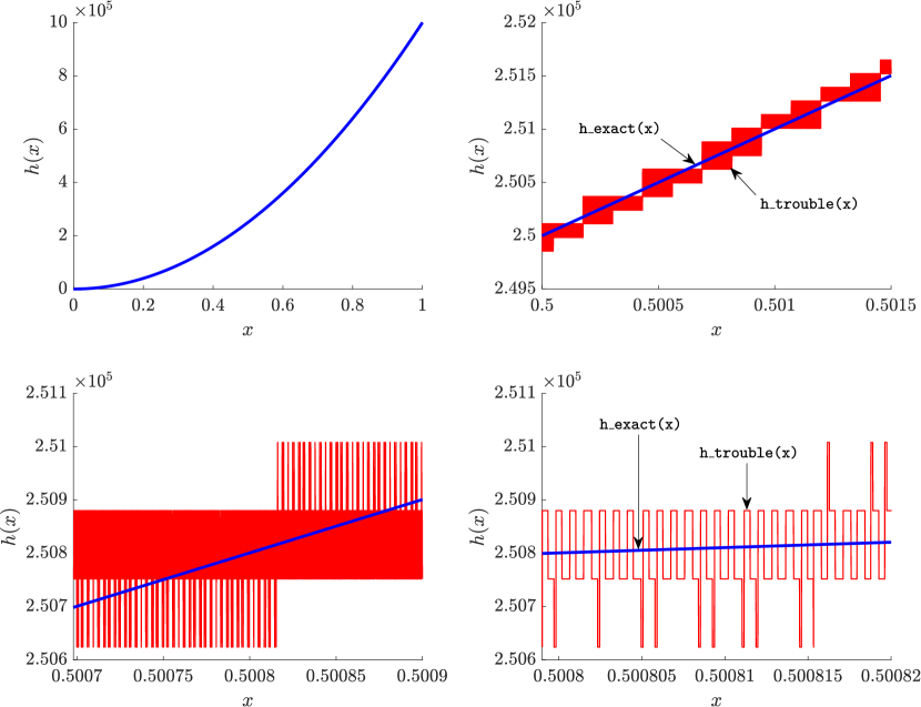
In Example 3.2, it is clear that the form of h_trouble(x) was implemented inefficiently and one should use the simpler form h_exact(x). However, in more complicated examples such a simplification is not always possible. The function of interest is the integrand $f(k)$ in (2). In the following we show that if it is inaccurately evaluated, we can observe similar misbehaviour as in the previous simple example. To avoid the problems with loosing significant digits, we perform the evaluation of function values also in the high precision arithmetic, in particular in vpa in MATLAB. All vpa values in this paper are obtained with 32 significant decimal digits precision.

From now on, the numerical analysis will involve only the AFSVJD model and the formula (2). In other SVJD models, very similar analysis can be performed with analogous switching regime setting (see below).

Example 3.3 (Global and local view to the integrand $f(k)$).

In Figures 2 and 3 we consider market data (European call options to FTSE 100 dated 8 January 2014, see (Pospíšil and Sobotka, 2016a) and Example 5.1 below)

$$\psi=(0.120548,6250,0.009,6721.8)$$

and demonstrate the numerical misbehaviour by changing only values of $\sigma$ and also the zoom depth, other parameters remain in each example the same. Whereas the inaccurately enumerated values are in double precision arithmetic (red in Figures 2 and 3), the smooth values are in vpa (blue). In Figure 2, bottom pictures for $\sigma=0.000001$, we can see that potential smoothing of the inaccurately evaluated integrand would not help, since it would be completely set off the exact values. Bottom right picture hence shows only the zoom of the double evaluated integrand from the bottom left picture.

\begin{overpic}[width=433.62pt]{fig1a} \put(25.0,40.0){\small$v=0.97$, $\kappa=17.6$, $\theta=0.95$, $\rho=-0.86$} \put(25.0,35.0){\small$\lambda=11.7$, $\mu_{J}=-6.66$, $\sigma_{J}=1.007$, $H=0.96$} \end{overpic}

\begin{overpic}[width=216.81pt]{fig1b}\put(40.0,24.0){\small$\sigma=0.0001$}\end{overpic}

\begin{overpic}[width=216.81pt]{fig1c}\put(40.0,24.0){\small$\sigma=0.00001$}\end{overpic}

\begin{overpic}[width=216.81pt]{fig1d}\put(40.0,24.0){\small$\sigma=0.000001$}\end{overpic}

\begin{overpic}[width=216.81pt]{fig1e}\put(40.0,24.0){\small$\sigma=0.000001$}\end{overpic}

Figure 2: Global and local view to the integrand $f(k)$ in Test Case 1.

\begin{overpic}[width=433.62pt]{fig2a} \put(25.0,40.0){\small$v=0.3$, $\kappa=5$, $\theta=0.1$, $\rho=-0.5$} \put(25.0,35.0){\small$\lambda=60$, $\mu_{J}=-9$, $\sigma_{J}=1.1$, $H=0.6$} \end{overpic}

\begin{overpic}[width=216.81pt]{fig2b}\put(40.0,24.0){\small$\sigma=0.001$}\end{overpic}

\begin{overpic}[width=216.81pt]{fig2c}\put(40.0,24.0){\small$\sigma=0.0001$}\end{overpic}

\begin{overpic}[width=216.81pt]{fig2d}\put(40.0,24.0){\small$\sigma=0.00001$}\end{overpic}

\begin{overpic}[width=216.81pt]{fig2e}\put(40.0,24.0){\small$\sigma=0.000001$}\end{overpic}

Figure 3: Global and local view to the integrand $f(k)$ in Test Case 2.

Moreover, inaccurately evaluated integrand can lead to really big differences in the option price, even in the order of hundreds of dollars.

Example 3.4 (Hundred dollars error).

For parameters

$$\chi =(0.98,8,0.8,0.000001,-0.75,0.75,1.4,0.2,0.9)$$

that can be observed during a calibration process and for data

$$\psi =(0.34,12500,0.017,10000)$$

we get

price_double=4115.317   price_vpa=3999.167   error=116.150
  int_double=1.48755534   int_vpa=1.51691623 error=0.02936088

where price denotes the value of the option price calculated using the Gauss-Kronrod(7,15) quadrature that is by default used in the function integral in MATLAB (we compare other numerical quadratures later in Section 4) and int denotes the value of the integral. The sub indices _double and _vpa denote that the value was obtained for integrand $f(k)$ evaluated using the standard double precision or vpa arithmetic respectively. Absolute difference error indicate a huge difference in the option price value.

In order to get a reasonable values in the calibration process, we need the integral to be calculated with the error less then 1e-8. The reason for this tolerance is the fact that in one calibration procedure, several hundred options are typically considered, which means that the utility (or fitness) function in the optimization procedure consists of this amount of integral evaluations and hence the option price calculation in each iteration. A safe option price value tolerance can be considered 1e-3. From the comparison of the error in integration and option price in the example above we can clearly see that in order to get the safe price within error 1e-3, we need integral to be calculated with error less then 1e-8.

It is worth to mention that the integrand $f(k)$ does not have to be evaluated in vpa for all parameter values. In fact, the most problematic cases occur only for rare certain combinations of parameters. In Table 3 we present an influence of one model parameter (in particular parameter $\sigma$) and approximation parameter $\varepsilon$ to the number of problematic cases. A problematic case is such that the integral was evaluated either with error greater than 1e-8, or with fevals greater than 1e4 (i.e. with high CPU time). Among all problematic cases, more than a third gave an error greater than 1e-2. Values in Table 3 show number of problematic cases in 10 millions random integral evaluations, parameter $\sigma$ is generated uniformly in different ranges with approximation parameter $\varepsilon$ being fixed in all corresponding trials. All other parameters are chosen uniformly random in bounds from Table 2. Influence of all parameters to the problematic cases follows below.

Table 3: Number of problematic cases in 10 millions random integral evaluations for different ranges for parameter $\sigma$ and different values of approximation parameter $\varepsilon$. All other parameters are chosen uniformly random in bounds from Table 2.

$\sigma\in\>\backslash\>\varepsilon=$	$10^{-3}$	$10^{-4}$	$10^{-5}$	$10^{-6}$
$[10^{-5};4]$	42	103	250	696
$[10^{-2};10^{-1}]$	0	0	155	7 315
$[10^{-3};10^{-2}]$	262	10 742	65 979	179 818
$[10^{-4};10^{-3}]$	109 922	269 021	418 708	528 910
$[10^{-5};10^{-4}]$	684 565	782 732	841 482	882 383
$[10^{-6};10^{-5}]$	1 059 632	1 064 681	1 068 015	1 071 241

To overcome the raised issues, we introduce a switching regime for problematic cases, i.e. in majority of cases, the evaluation will be done in standard double arithmetic, however, in problematic cases vpa arithmetic has to be used.

When analysing the integrand $f(k)$ in (2), we can find out that the order of magnitude in terms $C_{1}$ and $C_{2}$ can differ significantly. In fact, this difference is the core of the problem of inaccurately evaluated integrand. It is worth to mention that presented form of $C$ is the most numerically stable. Although it is possible to put the term in front of the logarithm into the exponent of the argument, which is mathematically equivalent, a presented form is numerically more suitable for finite precision arithmetic calculations. We introduce the following algorithm for the switching between the double and vpa evaluation of the integrand.

Let $\Re(z)$ denote the real part of a complex number $z$. Let $o_{1}$ and $o_{2}$ denote the order for the terms $C_{1}$ and $C_{2}$ respectively and $f_{0}$ be the value

$$f_{0}:=|\Re(f(0+i/2))|.$$ (5)

Then

$$o_{1} :=\log_{10}|\Re(C_{1})|,$$

$$o_{2} :=\log_{10}|\Re(C_{2})|,$$

$$o :=o_{1}-o_{2},$$

where we consider $\log_{10}(0)=-\infty$.

Numerical analysis results show that a problem occurs if $f_{0}$ is greater than $10^{-3}$ and the order difference $o$ is greater than $\omega_{0}=22$. If these two conditions hold, we have to switch the evaluation of the integrand from double to vpa. If $f_{0}>10^{-3}$ and $\sigma$ is really small, then $\Re(C_{2})$ is close to zero, the order difference $o=+\infty$ and we have to always switch. For values $f_{0}\leq 10^{-3}$, the values $f(k)$ remain close to zero for all $\Re(k)>0$ and they are correctly evaluated in double, so it is not necessary to switch to vpa and the integral will also be close to zero. Empirical value $\omega_{0}$ is determined by the values of the integrand $f(k)$ to be evaluated within precision 1e-5. Such a precision together with the exponential decay of the integrand allows us to evaluate the corresponding integral (2) numerically within precision 1e-8 (see numerical results in Section 5).

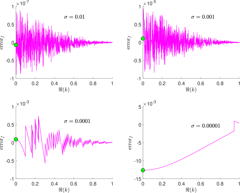
Example 3.5 (Test Case 1 revisited).

In Example 3.3 Figure 2 we presented inaccurately evaluated integrand for certain parameter values. In Table 4 we can see the relation of the order difference $o$ and the integrand evaluation error for different values of parameter $\sigma$, all other parameters remain the same. Values of $f_{0}$ are evaluated both in double or vpa and their difference is in the 7th column. In Figure 4 we can see an $\text{error}_{f}:=\Re(f^{\texttt{double}}(k)-f^{\texttt{vpa}}(k))$ for $\Re(k)\in[0,1]$. Maxima of these differences are listed in the last column of Table 4. We can see that the error for $o>22$ is bigger than the desired precision 1e-5.

Table 4: Integrand evaluation errors in Test Case 1

$\sigma$	$o_{1}$	$o_{2}$	$o$	$f_{0}^{\texttt{double}}$	$f_{0}^{\texttt{vpa}}$	$|f_{0}^{\texttt{double}}-f_{0}^{\texttt{vpa}}|$	$\max|\text{error}_{f}|$
0.1	5.061	-8.510	13.571	2.1369600154	2.1369600152	0.0000000001	0.0000000009
0.05	5.663	-9.112	14.775	2.1369590951	2.1369590940	0.0000000010	0.0000000034
0.01	7.061	-10.510	17.571	2.1369583500	2.1369583571	0.0000000070	0.0000000887
0.005	7.663	-11.112	18.775	2.1369583299	2.1369582649	0.0000000650	0.0000003834
0.001	9.061	-12.510	21.571	2.1369592635	2.1369581912	0.0000010722	0.0000093898
0.0005	9.663	-13.111	22.775	2.1369775046	2.1369581820	0.0000193225	0.0000378410
0.0001	11.061	-14.507	25.568	2.1370505356	2.1369581747	0.0000923609	0.0007385972
0.00005	11.663	-15.051	26.714	2.1388775265	2.1369581737	0.0019193527	0.0020950859
0.00001	13.061	-Inf	Inf	2.1243052036	2.1369581730	0.0126529693	0.0126529693

Figure 4: Integrand evaluation errors in Test Case 1 – see Example 3.5. Values are sampled at equidistant points with step-size 1e-3.

Further numerical analysis shows that it is not necessary to switch to vpa in all such cases and we can make some corrections to the empirical value $\omega_{0}$. The first correction is based on the order of the term in front of the integrand. The higher the order of this term, the higher order $o$ can lead to an integrand that is sufficient to be evaluated in standard double arithmetic (for simplicity we write that the integrand is “double sufficient”), i.e. it is not necessarily to switch to vpa. Since $Ke^{-r\tau}/\pi<K/3$, we define

$$\omega_{1}:=\min(5,\max(4-\log_{10}(K/3),0)).$$ (6)

The second correction is based on the order of the value $f_{0}$. Here the influence is reverse, the higher the value of the order of $f_{0}$, the worse is the behaviour of the integrand, i.e. the order $o$ must be lower in order for the integrand to be double sufficient. Let

$$\omega_{2}:=\min(\log_{10}|\Re(f_{0})|,0).$$ (7)

The overall switching regime algorithm is summarized as Algorithm 1 below. It is worth to mention that the switching criteria is relatively cheap operation that requires only one additional function evaluation, namely calculation of $f_{0}$ in double arithmetic. Additional speed-up of the algorithm could be achieved in faster calculation of the order of relevant terms, i.e. instead of calculating the decimal order using the base 10 logarithm, one could for example take the exponent from the floating point representation of the number. Such a modification goes beyond the scope of this manuscript.

  $o_{1}:=\log_{10}|\Re(C_{1})|$; $o_{2}:=\log_{10}|\Re(C_{2})|$; $o:=o_{1}-o_{2}$; $\omega_{0}=22$;

  $f_{0}:=f(0+i/2)$;

  par = false;

  if $f_{0}>10^{-3}$ and $o>\omega_{0}$ then

     $\omega_{1}:=\min(5,\max(4-\log_{10}(K/3),0))$;

     $\omega_{2}:=\min(\log_{10}|\Re(f_{0})|,0)$;

     if $o>\omega_{0}+\omega_{1}-\omega_{2}$ then

        par = true;

     end if

  end if

  if par then

     switch the evaluation of the integrand $f(k)$ from double to vpa

  end if

Algorithm 1 Fast regime switching algorithm for the evaluation of the integrand $f(k)$ that is by default in double.

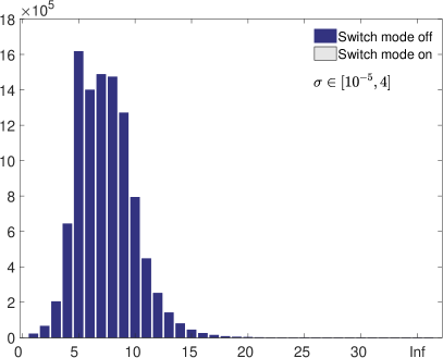
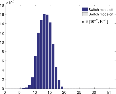
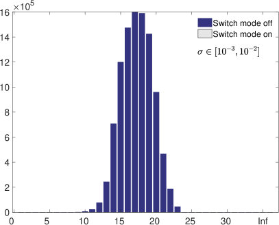
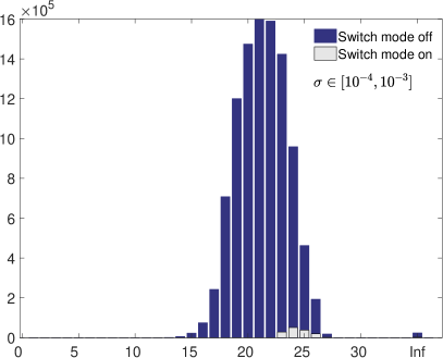
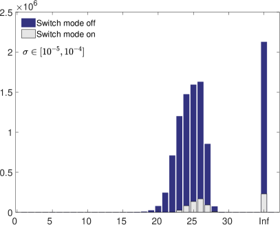
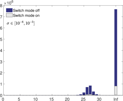
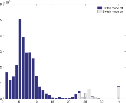
In Figure 5, we can see the histograms for the order difference $o$. In each case, 10 millions integral evaluations were performed with parameter values taken uniformly random in considered bounds. "Switch mode on" means that in the Algorithm 1 the value par = true. The lower the value of the parameter $\sigma$, the higher is the order difference $o$. However, as we can see, it is not only the value $\sigma$ that causes the problems. For many cases it is sufficient to evaluate the integrand $f(k)$ in double arithmetic only even if the value $\sigma$ is really low. In the last graph the value Inf indicate that the value $o=+\infty$, i.e. that $\Re(C_{2})$ is close to zero.

Note that histograms in Figure 5 correspond also to the values obtained in Table 3 and the thorough analysis of problematic cases motivated the choice of $\omega_{0}=22$ that can be observed also in histograms in the third row.

Figure 5: Influence of the parameter $\sigma$ to the switch mode. Horizontal axis shows the value of the order difference $o$, the vertical axis is the number of cases in 10 millions integral evaluations. All parameter values were generated uniformly random in considered bounds.

Example 3.6 (Problematic integrand evaluations during calibration).

Calibration of the models to real market data will be further studied below in Section 5.4. In this example we give more details to the number of problematic cases that occur during calibration processes described later in Example 5.1. Since the random generation of parameters occur only during the global optimization phase of the calibration process, we analyse the problematic integrand evaluations during this phase only.

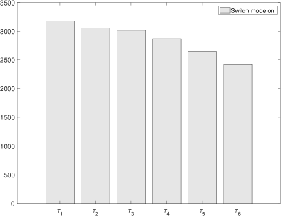
In particular, from ten independent global optimization runs for the AFSVJD model we gathered 3 034 000 different vectors of parameter values. For these vectors we tested if an integrand evaluation is double sufficient or not. We found out that there were 241 307 problematic cases, i.e. almost eight percent (7.95%). In Figure 6, we can see the double insufficiency distribution together with the dependence on the time to maturity (there are 6 different maturities in the data set ranging from $\tau_{1}=0.120548$ to $\tau_{6}=0.977528$). From this observation we can conclude that on average, more problematic cases occur for shorter maturities.

Figure 6: On the left, there is a histogram showing the double insufficiency during 10 independent global optimization runs. Horizontal axis shows the value of the order difference $o$, the vertical axis is the number of cases in 3 034 000 that were performed during the optimization. On the right, an average number of double insufficient integrand evaluations is grouped by the time to maturity $\tau$.

If the integrand is double insufficient and higher precision arithmetic is not used, the integral evaluation and hence the overall calibration process can slow down dramatically. Both accuracy and speed of the numerical quadratures will be thoroughly tested in the next section.

4 Numerical quadratures and their failures

The problem in numerical integration is to approximate definite integrals of the form $\int_{a}^{b}f(x)\,dx$ by the $n$-point numerical quadrature

$$\int_{a}^{b}f(x)\,\mathrm{d}x\approx Q_{n}[a,b]:=\sum_{i=1}^{n}w_{i}f(x_{i}),$$ (8)

where $w_{i}$ are the weights and $x_{i}$ are the points at which the function $f(x)$ is evaluated. An $n$-point Gaussian quadrature is a rule constructed to give an exact result for polynomials of degree $2n-1$ or less by a suitable choice of the points $x_{i}$ and weights $w_{i}$ for $i=1,\dots,n$. It can be shown Gautschi (2004); Press, Teukolsky, Vetterling, and Flannery (2007) that the evaluation points $x_{i}$ are the roots of a polynomial belonging to a class of orthogonal polynomials. Gauss-Legendre $n$-point quadrature (denoted by legendre($n$) below) is probably the best known Gaussian quadrature with associated orthogonal polynomials being the Legendre polynomials.

The adaptive control strategy divides the integration domain into subintervals, evaluates the integral at each region and uses an error estimate of the integral to check if a specified error tolerance is met. At regions where the function is well approximated by a polynomial, only a few function evaluations are needed, in other areas the adaptive strategy evaluates the subintervals in a recursive manner. Adaptive quadratures together with detailed error estimation techniques were reviewed by Gander and Gautschi (2000), where adaptive Simpson quadrature (quad) was also introduced. This review was recently extended by Gonnet (2009, 2012).

Adaptive strategy is applied also in the adaptive Gauss-Lobatto quadrature with a modification by the so called Kronrod extension to add an effective error control procedure. We consider two implementations of Gauss-Lobatto, namely adaptlob is the original implementation by Gander and Gautschi (2000) and quadl is the MATLAB implementation that further improves the adaptivity. The Lobatto formula has preassigned abscissas at the end points of the interval and other nodes and weights are determined in order to obtain the highest exactness possible. The Kronrod extension is used to provide an estimate of the approximation error. If the error exceeds a specified tolerance, regions where the function is not well behaved will be divided recurrently.

Gauss-Kronrod quadrature is an adaptive extension of the Gauss-Legendre algorithm in which the evaluation points are chosen so that an accurate approximation can be computed by re-using the information produced by the computation of a less accurate approximation. For the same set of function evaluation points, it has two quadrature rules, one higher order and an embedded one with lower order. The difference between these two approximations is used to estimate the calculation error of the integration. If the quadrature is applied to the interval $[a_{k},b_{k}]$, then the error estimate takes the form

$$E_{k}=|G_{n}[a_{k},b_{k}]-K_{2n+1}[a_{k},b_{k}]|,$$ (9)

where $G_{n}[a,b]$ is the $n$-point Gauss quadrature rule of degree $2n-1$, and $K_{2n+1}[a,b]$ is the $2n+1$ point Gauss-Kronrod extension of degree $3n+1$ that is used as the approximation of the integral. This is also the error estimate currently used in the MATLAB function integral that implements the adaptive Gauss-Kronrod(7,15) quadrature. This quadrature was chosen as the reference, since it is used de facto as an industrial standard in the latest releases of MATLAB. Initially, the interval $[a,b]$ is split into 10 equally sized subintervals. The default recurrence rule is set so that if the error estimate (9) for an interval $[a_{k},b_{k}]$ is greater than the prescribed tolerance, the interval $[a_{k},b_{k}]$ is divided to halves where the process is recurrently repeated. A reference to Gauss-Kronrod quadratures is Gautschi (1988), computation of Gauss-type quadrature formulas is further studied for example in Laurie (2001). It is worth to mention that other error estimates for the Gauss-Kronrod quadrature exist, some of them are of rather curious empirical character (e.g. the one used in the widely-used QUADPACK library, cf. (Gonnet, 2012, Section 2.4)), but in principle none of the estimates can properly handle the problem of loosing significant digits precision in the inaccurate integrand evaluation. This problem leads us to another simple example showing the failure of numerical quadratures, in particular of the adaptive Gauss-Kronrod quadrature.

Example 4.1 (Failure of the Gauss-Kronrod quadrature).

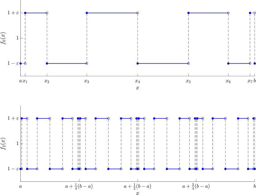
Let $f_{0}(x)$ be a piecewise constant function taking values either $1-\varepsilon$ or $1+\varepsilon$ with discontinuities exactly at the quadrature abscissas so that $\int\limits_{a}^{b}f_{0}(x)\,\mathrm{d}x=b-a$, see Figure 7 at the top where discontinuities occur at the abscissas of the Gauss-Kronrod(3,7) quadrature. The value of $\varepsilon$ is sufficiently small in order to serve as a measure of discontinuities caused by loosing significant digits. Let us consider the general Gauss-Kronrod($n$,$2n+1$) quadrature. The even nodes that partition the interval $[a,b]$ are the Gaussian points of the $G_{n}[a,b]$ quadrature and $f_{0}$ is equal to $1-\varepsilon$ at these points and $1+\varepsilon$ at the odd nodes that are the Gaussian points of the Kronrod extension $K_{2n+1}[a,b]$. We have that

$$G_{n}[a,b] =\sum_{i=1}^{n}w_{i}^{G}f_{0}(x_{i}^{G})=(1-\varepsilon)\sum_{i=1}^{n}w_{i}^{G}=(1-\varepsilon)(b-a)$$

$$K_{2n+1}[a,b] =\sum_{i=1}^{2n+1}w_{i}^{K}f_{0}(x_{i}^{K})=\sum_{i=1}^{n}w_{2i+1}^{K}f_{0}(x_{2i+1}^{K})+\sum_{i=1}^{n}w_{2i}^{K}f_{0}(x_{2i}^{K})$$

$$=(1+\varepsilon)\sum_{i=1}^{n}w_{2i+1}^{K}+(1-\varepsilon)\sum_{i=1}^{n}w_{2i}^{K}=\sum_{i=1}^{2n+1}w_{i}^{K}+\varepsilon\left(\sum_{i=1}^{n}w_{2i+1}^{K}-\sum_{i=1}^{n}w_{2i}^{K}\right)$$

$$=b-a+\varepsilon(b-a)C_{n}=(b-a)(1+\varepsilon C_{n})$$

and the error estimate

$$E_{0} =|G_{n}[a,b]-K_{2n+1}[a,b]|=|(1-\varepsilon)(b-a)-(b-a)(1+\varepsilon C_{n})|$$

$$=\varepsilon(b-a)\tilde{C}_{n}.$$

For example for $\varepsilon=10^{-4}$, $n=7$ (i.e. for Gauss-Kronrod(7,15) quadrature) and $[a,b]=[-1,1]$ we get $E_{0}\doteq 2.004652\times 10^{-4}$ which is much bigger than the default absolute or relative tolerance AbsTol=1e-10 and RelTol=1e-6 respectively and hence the adaptive refinement is required.

To mimic the inaccurate evaluation of a function caused by loosing significant digits, we can consider a piecewise constant function $f_{l}(x)$ taking again values either $1-\varepsilon$ or $1+\varepsilon$ with discontinuities at the quadrature abscissas in all of the $2^{l}$ subintervals $\left[a+\frac{i-1}{2^{l}}(b-a),a+\frac{i}{2^{l}}(b-a)\right]$, $i=1,\dots,2^{l}$. In Figure 7 at the bottom we can see a graph of function $f_{2}$, i.e. the case where the original interval $[a,b]$ was divided into 4 subintervals and at each of the subinterval the discontinuities occur at the seven abscissas of the Gauss-Kronrod(3,7) quadrature. To approximate the exact value $\int\limits_{a}^{b}f_{l}(x)\,\mathrm{d}x=b-a$ by the adaptive Gauss-Kronrod($n$,$2n+1$) quadrature, adaptive refinement must be performed at least to the $2^{l+1}$ subintervals, where the local error at the level $2^{l}$ is $E_{0}$.

Figure 7: Functions $f_{0}$ and $f_{2}$ from the Example 4.1. Discontinuities occur at the abscissas of the Gauss-Kronrod(3,7) quadrature.

Example 4.2 (Test Case 1 revisited).

In Example 3.3 Figure 2 we presented inaccurately evaluated integrand for certain parameter values that could be obtained during the calibration process. Examining the integrand for these parameter values, we can find out that in double evaluation there were $63\,302$ “significant discontinuities” of $f(k)$ for $\Re(k)\in[0,20]$ with jump sizes up to $8.6846\times 10^{-4}$ (average jump size $1.9082\times 10^{-6}$). To satisfy the local Gauss-Kronrod error estimate to be within the relative error $10^{-6}$, adaptive refinement had to be done down to the interval length $5\times 10^{-8}$. In the language of the previous Example 4.1, the value of $l$ can grow up to 12–16. Not only is such a numerical integration time demanding (one integral can be calculated several seconds, for exact values see results in Section 5), the obtained integral value is far from the precise value, the error is $2.4679\times 10^{-5}$ although the adaptive quadrature ends with errors within the default tolerances AbsTol=1e-10 and RelTol=1e-6.

From the review of the adaptive quadratures written by Gonnet (2009, 2012) it is obvious that although many other error estimates exist, none of them can properly handle the inaccuracy of the function evaluation caused by loosing significant digits. Almost all existing error estimates assume that the integrand is sufficiently smooth. The only exception is probably the CADRE estimate by de Boor (see (Gonnet, 2012, Section 3.1)) that allows to detect the low frequency discontinuities. Although the integrand in our case is theoretically sufficiently smooth, for some parameter values its evaluation is numerically double insufficient. The only way how to calculate the integral of such an integrand is to use the high precision arithmetic. Much simpler integrand is for example studied by Gautschi (2016) who introduces a non-standard Gauss-Hermite quadrature with empirical error estimates and implementation Gautschi (2017) using the MATLAB vpa.

In the numerical comparison provided in the next section, integral (vpa) denotes the case when the function integral is applied to vpa evaluated integrand, i.e. the quadrature uses values that are evaluated in vpa and converted to double. In the MATLAB release R2016b, a new function vpaintegral was introduced. This function implements a semi-symbolic quadrature that is supposed to be the high-precision numerical integration. Although the way how this quadrature obtains the numerical result differs from all other studied quadratures, we also consider it in our comparisons. For convenience we also add the very simple trapezoidal rule (trapz) that together with legendre is not adaptive. To understand how the adaptivity works in all considered quadratures is crucial to realize what happens in a numerical quadrature if the integrand is inaccurately evaluated as we saw for example in Figures 2 and 3.

5 Numerical results

In this section we compare numerical quadratures behaviour in problematic cases and with the implementation of the switching regime Algorithm 1 described in Section 3.

We measure an average calculation time (reference PC with 1x quad-core Intel i7-4770K 3.5 GHz CPU and 16 GB RAM) and number of integrand evaluations (fevals). Interesting results are highlighted. In all quadratures we set the tolerances to satisfy requirements mentioned in Section 3, i.e. we set absolute tolerance to be AbsTol=1e-10 and relative tolerance RelTol=1e-6.

5.1 Quadratures behaviour in problematic cases

In Table 5 we can see quadratures comparison for numerical integration with parameter values taken from test case 1, see Figure 2. Although the global view to the integrand does not indicate any potential problem, the contrary is true. We compare several quadratures for double evaluated integrand with reference value integral (vpa), i.e. integral function applied to the vpa evaluated integrand. In fact, the whole integrand $f(k)$ is evaluated using vpa and before plugging it into the integral function, it is converted into double. For convenience, we also provide the simple trapz rule with step sizes 0.01 and 0.001 and quadl all for double or vpa evaluated integrand.

In the case for $\sigma=0.001$, apart from quadl errors for all other quadratures are negligible, as well as computation times (without vpa) and fevals are small. Also quadl (vpa) give us accurate result (in given tolerance 1e-8). From the integral and integral (vpa) comparison we can see that even in this example the value differs. Computation time for vpa is ca 100 times higher which goes against our requirement to calculate the integral quickly. We can see that using vpa evaluated integrand in this case is not necessary for integral, but it is necessary for quadl. Computation times are especially huge for trapz (vpa).

A problematic case occurs if we change $\sigma$ to $0.0001$. Errors for all quadratures increase due to the inaccurately evaluated integrands. Computation time for integral is larger than in the previous case and it is actually larger than for integral (vpa), which is caused by enormous fevals increase. Such a huge increase is caused by the adaptivity of the quadrature applied to the inaccurately evaluated integrand.

Further decrease of $\sigma$ to $0.00001$ causes further error increase for all quadratures. Although one could expect larger computation time and fevals, these values for integral are much smaller than in the previous case, but error is much larger. Even if the computation time is low, there can be still a problematic case with high precision error and one can recognize it by large fevals. This is the reason why one of our criteria for problematic cases is fevals larger than 1e4.

From all three trials we learned that if we use vpa, fevals remain the same and as well as the computation times are very similar. This is an important indicator that the problematic cases are caused by the inaccurately evaluated integrands.

Table 5: Quadratures comparison for Test Case 1

method (case $\sigma=0.001$)	value	error	time [s]	fevals
integral	0.77681485	0.00000006	0.056	300
integral (vpa)	0.77681478	0.00000000	4.948	270
legendre (128)	0.77680533	0.00000944	0.006	64
legendre (256)	0.77682245	0.00000767	0.013	128
quad	0.77681499	0.00000020	0.092	1694
quadl	0.94027672	0.16346193	0.150	2018
quadl (vpa)	0.77681478	0.00000000	4.110	146
adaptlob	0.77681496	0.00000017	1.485	30734
trapz (0.01)	0.77681499	0.00000021	0.014	1
trapz (0.001)	0.77681499	0.00000020	0.027	1
trapz (vpa, 0.01)	0.77681478	0.00000000	14.287	1
trapz (vpa, 0.001)	0.77681478	0.00000000	301.293	1
method (case $\sigma=0.0001$)	value	error	time [s]	fevals
integral	0.77683946	0.00002467	6.761	360780
integral (vpa)	0.77681478	0.00000000	4.872	270
legendre (128)	0.77695229	0.00013750	0.006	64
legendre (256)	0.77682884	0.00001405	0.012	128
quad	0.77688362	0.00006883	0.218	5006
quadl	0.75020018	0.02661460	0.146	2030
quadl (vpa)	0.77681478	0.00000000	4.101	146
adaptlob	0.77684007	0.00002528	2.278	47324
trapz (0.01)	0.77684249	0.00002770	0.010	1
trapz (0.001)	0.77683949	0.00002470	0.029	1
trapz (vpa, 0.01)	0.77681478	0.00000000	13.743	1
trapz (vpa, 0.001)	0.77681478	0.00000000	288.313	1
method (case $\sigma=0.00001$)	value	error	time [s]	fevals
integral	0.76823548	0.00857930	0.655	28260
integral (vpa)	0.77681478	0.00000000	5.004	270
legendre (128)	0.76877555	0.00803923	0.007	64
legendre (256)	0.76810697	0.00870781	0.015	128
quad	0.76823622	0.00857856	0.099	2022
quadl	0.76846917	0.00834561	0.149	2018
quadl (vpa)	0.77681478	0.00000000	4.084	146
adaptlob	0.76823478	0.00858000	0.216	4232
trapz (0.01)	0.76828142	0.00853336	0.013	1
trapz (0.001)	0.76823697	0.00857781	0.030	1
trapz (vpa, 0.01)	0.77681478	0.00000000	14.618	1
trapz (vpa, 0.001)	0.77681478	0.00000000	310.098	1

5.2 Results for switching regime

In this section we apply the switching regime Algorithm 1 to the function integral, i.e. for problematic cases the quadrature is applied to the vpa evaluated integrand and in other cases standard double arithmetic is used. The comparison is summarized in Table 6. As we can see, the error increases for smaller values of parameter $\sigma$ which is caused by the increasing order difference $o$.

In Test Case 1 we can observe that a problem starts to emerge even for larger value of $\sigma=0.001$, see the first double-row where the fevals difference is already 30, although this case does not fall into the problematic category, the error is low and it is actually not necessary to switch to vpa. In other cases the difference in fevals is huge, apart from the last case when the error was large. In Test Case 2 for $\sigma=0.00001$ the error is negligible in given tolerance 1e-8, however this must be interpreted as a coincidence, because the fevals for integral without vpa is huge.

The obtained values confirm the choice of the value $\omega_{0}=22$ in the switching regime Algorithm 1 as well as they correspond to the choice of correction terms $\omega_{1}$ and $\omega_{2}$ whose influence was described in detail in Section 3. It is useful to remind that the Algorithm 1 is designed to be fast, i.e. for some rare parameter values it can happen that the algorithm switches to the vpa evaluation of the integrand even if it is double sufficient, however the algorithm should not forget to switch any problematic case which makes the algorithm fast and reliable.

Table 6: Using switching regime integral in Test Case 1 and 2

$\sigma$	$o$	$\omega_{1}$	par	integral  /   integral (vpa)			error
	$f_{0}$	$\omega_{2}$		value	time	fevals
Test Case 1 (see Figure 2)
0.001	21.572	–	false	0.77681485	0.056	300	0.00000006
	2.137	–		0.77681478	4.948	270
0.0005	22.775	0.681	true	0.77681452	4.241	115320	0.00000025
	2.137	0		0.77681478	2.244	270
0.0001	25.568	0.681	true	0.77683946	6.761	360780	0.00002467
	2.1371	0		0.77681478	4.872	270
0.00005	26.715	0.681	true	0.77684142	4.198	217170	0.00002663
	2.1389	0		0.77681478	5.056	270
0.00001	Inf	0.681	true	0.76823548	0.655	28260	0.00857930
	2.1243	0		0.77681478	5.004	270
0.000001	Inf	0.681	true	0.77674994	0.068	750	0.00006484
	2.1243	0		0.77681478	5.043	270
Test Case 2 (see Figure 3)
0.0001	20.447	–	false	0.00695940	0.066	900	0.00000000
	0.12193	–		0.00695940	16.198	900
0.00005	21.651	–	false	0.00695940	0.066	900	0.00000000
	0.12193	–		0.00695940	16.105	900
0.00001	24.447	0.681	true	0.00695940	5.901	312240	0.00000000
	0.12193	-0.914		0.00695940	16.118	900
0.000001	28.555	0.681	true	0.00695451	10.316	561750	0.00000489
	0.12193	-0.914		0.00695940	16.132	900

5.3 Optimal switching regime quadratures

So far the whole calculation of $f(k)$ was either performed in double or vpa arithmetic. Since the vpa is rather time consuming, additional speed-up (denoted by opt in tables below) can be achieved by further implementation improvements. Since the most problematic part of $f(k)$ is the term $C(k,\tau)$, we can calculate precisely (using vpa) only this term $C$ and then convert it to double. The remaining terms are double sufficient.

Let us now compare numerical quadrature in cases when we have to switch to the vpa evaluation of the integrand. In Tables 7 and 8 we can see all such cases that we already met in Table 6 now for different numerical quadratures. Using check mark ✓ we indicate that the quadrature gave us the accurate result (in given tolerance 1e-8) with respect to the reference value obtained by the integral (vpa), i.e. using the double precision arithmetic function integral applied to the precisely evaluated integrand (i.e. to integrand evaluated using vpa and converted back to double). The last row in each block shows the results for the semi-symbolic quadrature vpaintegral that is supposed to be the implementation if the high-precision numerical integration. Since the way how vpaintegral evaluates the integrand differs from all other numerical quadratures, the number of fevals in Tables 7 and 8 is omitted for this quadrature.

We can see that for all numerical quadratures computational time is proportional to fevals. In all cases we also got a desirable accuracy with the only exception quad in Test Case 2. From this point of view, results for all numerical quadratures are comparable. On the other hand, the semi-symbolic quadrature vpaintegral seems to be unusable and although its idea seems to be promising for the future, in its current state we cannot recommend its usage. First of all, even for the same tolerance setting (AbsTol=1e-10, RelTol=1e-6) it does not satisfy our precision criteria. Moreover, we can observe that the error of vpaintegral somehow correlates to the error of integral without vpa, i.e. to only double evaluated integrand and double calculated integral. Such a correlation indicate probably a systematic misbehaviour of vpaintegral.

To sum up the comparison results for other numerical quadratures, in all our tests the quadl (opt) quadrature performed best, since it needed fewest fevals and hence it was fastest in all our examples. However, as we saw in Table 5, it can have serious problems in the cases that are not switched to vpa, i.e. in cases where integrand is double sufficient. Since all other quadratures are time comparable as well and the differences are not big, we can conclude that the reference Gauss-Kronrod quadrature represented by the integral (opt) was chosen reasonably.

Table 7: Using optimal switching regime quadratures in Test Case 1

method		value	error	time [s]	fevals
($\sigma=0.0005$, $o=22.775$, $f_{0}=2.137$, $\omega_{1}=0.681$, $\omega_{2}=0$, par = true)
integral		0.77681452	0.00000025	2.244	115380
integral (vpa)		0.77681478	0.00000000	4.920	270
integral (opt)	✓	0.77681478	0.00000000	4.157	270
quad (opt)	✓	0.77681478	0.00000000	6.206	304
quadl (opt)	✓	0.77681478	0.00000000	3.520	146
adaptlob (opt)	✓	0.77681478	0.00000000	3.668	164
vpaintegral		0.77681305	0.00000172	7.694	-
($\sigma=0.0001$, $o=25.568$, $f_{0}=2.1371$, $\omega_{1}=0.681$, $\omega_{2}=0$, par = true)
integral		0.77683946	0.00002467	6.761	360780
integral (vpa)		0.77681478	0.00000000	4.872	270
integral (opt)	✓	0.77681478	0.00000000	4.112	270
quad (opt)	✓	0.77681478	0.00000000	6.270	304
quadl (opt)	✓	0.77681478	0.00000000	3.520	146
adaptlob (opt)	✓	0.77681478	0.00000000	3.467	164
vpaintegral		0.77685918	0.00004440	31.627	-
($\sigma=0.00005$, $o=26.715$, $f_{0}=2.1389$, $\omega_{1}=0.681$, $\omega_{2}=0$, par = true)
integral		0.77684142	0.00002663	4.198	217170
integral (vpa)		0.77681478	0.00000000	5.056	270
integral (opt)	✓	0.77681478	0.00000000	4.165	270
quad (opt)	✓	0.77681478	0.00000000	6.317	304
quadl (opt)	✓	0.77681478	0.00000000	3.615	146
adaptlob (opt)	✓	0.77681478	0.00000000	3.480	164
vpaintegral		0.77682241	0.00000762	31.843	-
($\sigma=0.00001$, $o=\mathrm{{\tt Inf}}$, $f_{0}=2.1243$, $\omega_{1}=0.681$, $\omega_{2}=0$, par = true)
integral		0.76823548	0.00857930	0.655	28260
integral (vpa)		0.77681478	0.00000000	5.004	270
integral (opt)	✓	0.77681478	0.00000000	4.108	270
quad (opt)	✓	0.77681478	0.00000000	6.391	304
quadl (opt)	✓	0.77681478	0.00000000	3.594	146
adaptlob (opt)	✓	0.77681478	0.00000000	3.582	164
vpaintegral		0.76839158	0.0084231	13.270	-
($\sigma=0.000001$, $o=\mathrm{{\tt Inf}}$, $f_{0}=2.1243$, $\omega_{1}=0.681$, $\omega_{2}=0$, par = true)
integral		0.77674994	0.00006484	0.068	750
integral (vpa)		0.77681478	0.00000000	5.043	270
integral (opt)	✓	0.77681478	0.00000000	4.086	270
quad (opt)	✓	0.77681478	0.00000000	6.233	304
quadl (opt)	✓	0.77681478	0.00000000	3.516	146
adaptlob (opt)	✓	0.77681478	0.00000000	3.515	164
vpaintegral		0.77747608	0.00066129	1.016	-

Table 8: Using optimal switching regime quadratures in Test Case 2

method		value	error	time [s]	fevals
($\sigma=0.00001$, $o=24.447$, $f_{0}=0.12193$, $\omega_{1}=0.681$, $\omega_{2}=-0.914$, par = true)
integral		0.00695940	0.00000000	5.901	312240
integral (vpa)		0.00695940	0.00000000	16.118	900
integral (opt)	✓	0.00695940	0.00000000	13.367	900
quad (opt)		0.00695930	0.00000010	12.691	622
quadl (opt)	✓	0.00695940	0.00000000	8.639	362
adaptlob (opt)	✓	0.00695940	0.00000000	15.986	686
vpaintegral	✓	0.00695940	0.00000000	4.752	-
($\sigma=0.000001$, $o=28.555$, $f_{0}=0.12193$, $\omega_{1}=0.681$, $\omega_{2}=-0.914$, par = true)
integral		0.00695451	0.00000489	10.316	561750
integral (vpa)		0.00695940	0.00000000	16.132	900
integral (opt)	✓	0.00695940	0.00000000	13.348	900
quad (opt)		0.00695930	0.00000010	12.894	622
quadl (opt)	✓	0.00695940	0.00000000	8.614	362
adaptlob (opt)	✓	0.00695940	0.00000000	16.104	686
vpaintegral		0.00695490	0.00000449	22.478	-

5.4 Calibration to real market data

The problem of calibration of the model to real market data is formulated as the nonlinear least squares optimization problem,

$$\inf\limits_{\chi}G(\chi),\hskip 8.5359ptG(\chi)=\sum^{N}_{i=1}w_{i}|C_{i}^{\chi}(T_{i},K_{i})-C_{i}^{*}(T_{i},K_{i})|^{2},$$

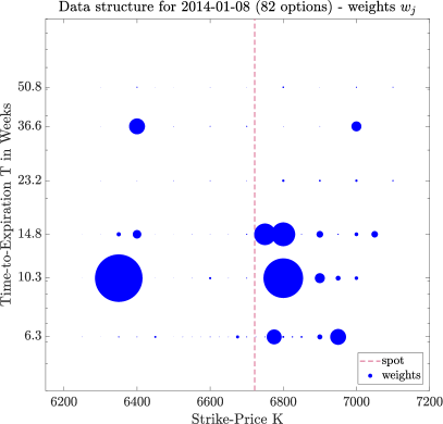
where $N$ denotes the number of observed option prices, $C^{*}_{i}(T_{i},K_{i})$ is the market price of the call option, $C^{\chi}_{i}$ denotes the model price of the $i$-th option computed using formula (2) evaluated with the vector of model parameters $\chi$, and $w_{i}$ is the $i$-th weight proportional to the bid-ask spread $\delta_{i}>0$. In particular we consider the following weights (Mrázek, Pospíšil, and Sobotka, 2016)

$$w_{i}=\frac{\delta_{i}^{-2}}{\sum\limits_{j=1}^{N}\delta_{j}^{-2}},\quad i=1,\dots,N.$$

In Section 2 we mentioned that for the AFSVJD (Pospíšil and Sobotka, 2016a; Mrázek, Pospíšil, and Sobotka, 2016) model, the vector of model parameters is $\chi=(v_{0},\kappa,\theta,\sigma,\rho,\lambda,\mu_{J},\sigma_{J},H)$. If not stated otherwise, the optimization will be performed with simple bounds from Table 2 and with fixed approximation parameter $\varepsilon=10^{-6}$. Since the AFSVJD model covers also several other widely used models, we will consider also the case when $H=0.5$, i.e. the Bates (1996) model with 8 parameters $(v_{0},\kappa,\theta,\sigma,\rho,\lambda,\mu_{J},\sigma_{J})$ and further with $\lambda=0$, i.e. the Heston (1993) model with 5 parameters $(v_{0},\kappa,\theta,\sigma,\rho)$.

To evaluate the calibration performance, we measure the maximum and average of absolute (value of) relative error

$$\text{MARE}(\chi)=\max_{i=1,\dots,N}\frac{|C_{i}^{\chi}-C_{i}^{*}|}{C_{i}^{*}},\qquad\text{AARE}(\chi)=\frac{1}{N}\sum_{i=1}^{N}\frac{|C_{i}^{\chi}-C_{i}^{*}|}{C_{i}^{*}}.$$

Following the widely accepted recommendations (Pospíšil and Sobotka, 2016a, b; Mrázek, Pospíšil, and Sobotka, 2016; Mrázek and Pospíšil, 2017) we perform the calibration as a combination of the global and local optimization techniques. Global optimization part of the calibration is especially needed when there is no suitable initial guess for the gradient based method used in the local optimizer. For the global optimizer we choose the genetic algorithm (GA) with the standard setting: EliteCount 5% of population size, intermediate crossover (creates children by taking a random average of the parents) with CrossoverFraction 80% (of the population at the next generation, not including elite children), no migration, uniform selection and Gaussian mutation. For the local optimizer we choose the standard trust-region-reflective Newton gradient method for nonlinear least squares (LSQ) with stopping criteria set to function value tolerance or step tolerance 1e-9. Calibration process is therefore performed in two steps:

Step 1:

Run 20 iterations (generations) of the GA optimization for utility (fitness) function $G(\chi)$, GA is run with population size 200.

Step 2:

Run the LSQ optimization, the optimization is run with the initial guess obtained as a solution from the previous step.

In the following example, we are especially interested in comparison of calibration results when the integral in formula (2) is evaluated if our proposed switching algorithm is implemented or if it is not used at all.

Example 5.1.

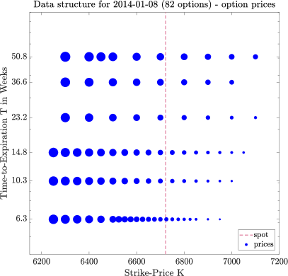
Let us consider a data set of 82 traded European call options to the index FTSE 100 dated 8 January 2014, see (Pospíšil and Sobotka, 2016a). In Figure 8 we can see the option data structure. There are six different time to maturities ranging from $0.120548$ to $0.977528$ (in years) with strikes ranging from 6 250 to 7 100 with spot price 6 721.78. In Table 9 we can see a comparison of measured errors for all three models in two different regimes, either our fast regime switching algorithm is implemented (’ON’, we use the integral (opt) variant from the previous section) or not used at all (’OFF’).

As we can see, in both SVJD models (AFSVJD and Bates model) we get better calibration results if our switching algorithm is used. For Heston model we also get slightly better results, but the measured errors are indistinguishable within the tolerance 1e-9. The table shows also the ratio how many times the evaluation of the integrand had to be switched to vpa from all integral calculations in each calibration task. The integral implementation is array valued, i.e. one integral calculation is performed at once for all 82 option data combinations. For convenience, we set the lower bound for parameter $\sigma$ to 1e-4 (i.e. to a value 1 bps = 0.01 % usually used in practice). For curiosity we also include a case for AFSVJD model, where we set the lower bound for parameter $\sigma$ to 1e-2 only. As we can see, although the resulting calibrated value of parameter $\sigma$ is far from zero, avoiding the values smaller than 1e-2 during the optimization process led to a worse calibration result. On the other hand, the results 7 and 8 are almost indistinguishable within the tolerance 1e-9 since there were only 25 (in 4792) problematic situations when the integrand had to be switched to vpa and fortunately the final result was not affected in this case. Among all results, the 6th calibration trial gives the best results also in terms of AARE.

Figure 8: Option data structure for data from Example 5.1. There are 82 options in considered data set of European call options to FTSE 100 dated 8 January 2014. Option prices are depicted on the left and considered calibration weights on the right. Note that the scaling of dot diameters differ in both pictures just for visual purposes, the diameters on the left are proportional to the option prices (USD), whereas on the right they are proportional to the unit-less weights.

Table 9: Calibration results for data from Example 5.1 for different models with switching regime algorithm (switch) used (ON) or not (OFF). Dimension (dim.) indicate the length of the vector of model parameters $\chi$ that is being calibrated. Number of switches (# of sw.) indicate, how many times the evaluation of the integrand had to be switched to vpa in all integrand evaluations in each calibration trial. Calibrated parameter values for the AFSVJD model are listed below the table.

model	dim.	switch	# of sw.	$\text{AARE}(\chi_{i})$	$\text{MARE}(\chi_{i})$	$G(\chi_{i})$	$i$
Heston	5	OFF	0 / 4508	0.06512446	0.35292408	106.94072000	1
		ON	74 / 4442	0.06512469	0.35292146	106.94071999	2
Bates	8	OFF	0 / 4364	0.10001985	0.92693868	130.25382485	3
		ON	293 / 4526	0.06512521	0.35292381	106.94071992	4
AFSVJD	9	OFF	0 / 4812	0.06512390	0.35292162	106.94072035	5
		ON	88 / 6162	0.06065231	0.42843860	84.14079714	6
AFSVJD	9	OFF	0 / 4792	0.06512324	0.35291189	106.94071997	7
($\sigma\geq 0.01$)		ON	25 / 4792	0.06512324	0.35291189	106.94071997	8

$$\chi_{5} =(0.00644592,6.19473908,0.00880072,3.95726677,0.99999999,0.00000000,1.04059997,1.61568883,0.69621767)$$

$$\chi_{6} =(0.00001000,0.00716856,0.18471466,3.71676726,0.99995279,3.49596838,0.04460999,0.00001000,0.64278280)$$

$$\chi_{7} =(0.00644589,6.19756427,0.00880014,3.23167264,0.99999999,0.00000246,-7.44129841,2.73418003,0.68154330)$$

$$\chi_{8} =(0.00644589,6.19756427,0.00880014,3.23167264,0.99999999,0.00000246,-7.44129841,2.73418003,0.68154330)$$

6 Conclusion

In this paper we studied numerical integration in semi-closed option pricing formulas used especially in jump diffusion stochastic volatility models. When calibrating these models to real market data, a numerical calculation of integrals has to be performed many times for different model parameters. During calibration process all integral evaluations have to be performed with high precision and low computational time requirements. Motivation for writing this paper was an observation that for some model parameters, many numerical quadrature algorithms fail to meet these requirements. We observed an enormous increase in function evaluations (fevals) especially in adaptive quadratures, serious precision problems even for the simple trapezoidal rule as well as a significant increase of computational time in all quadratures. At first we thought that the problem is in the choice of numerical quadrature. However, a more detailed numerical analysis showed that the problem is caused especially by the inaccurately evaluated integrand. We demonstrated this behaviour on a simplified integrand in conference paper Daněk and Pospíšil (2015) and suggested the usage of variable precision arithmetic (vpa) in all cases when evaluating the integrand in standard double arithmetic is not sufficient.

The aim of this paper was to numerically analyse the integrand in the approximative fractional stochastic volatility jump diffusion model first introduced by Pospíšil and Sobotka (2016a) that among others cover also the Bates and Heston models. Since the evaluation of the integrand in vpa is time consuming, the goal was to find a suitable fast algorithm that could tell if the integrand is double sufficient or if it has to be evaluated in higher precision. The main result of this paper is therefore the Algorithm 1. Experimental results then cover comparison of numerical quadratures especially for problematic (double insufficient) cases that has to be switched to vpa.

From all numerical experiments we learned several lessons. First of all, a thorough numerical analysis is a necessity in all problems that require some numerics, one should not believe any implementation of any formula if not tested thoroughly. Even a very nice looking integrand can cause serious numerical problems especially if inaccurately evaluated which can of course be hard to realize. Blindly used formulas that were not numerically analysed can lead to potential big losses as we showed in the example of wrongly priced option with difference greater than 100 dollars. We also learned that a small error of the numerical integration can be actually a coincidence and the potential problems can be detected by monitoring the number of fevals. And last but not least, it was not only the low value of parameter $\sigma$ that causes the problematic cases although its influence is the most remarkable.

To tell what numerical quadrature is the best for our studied integral is not an easy task, since the behaviour differs in double sufficient and problematic cases. In fact, when working with real data, we might find a case when every numerical quadrature fails to meet some criteria. Based on our huge number of experiments we can recommend the Gauss-Kronrod(7,15) quadrature implemented in MATLAB as a function integral together with the correct (opt) implementation of the regime switching Algorithm 1.

A promising for the future is the idea of high-precision numerical quadrature, newly available in MATLAB function vpaintegral that can for example precisely calculate simple integrands such as the one in Daněk and Pospíšil (2015), but as we showed still has some serious problems with the integrand studied in this paper. To have a robust implementation of such a high-precision integration routine can be in fact a challenging issue, as was mentioned by Bailey, Jeyabalan, and Li (2005) where several high-precision quadratures are compared on a set of test problems with integrands much simpler than the one studied here.

Last but not least, we compared the calibration results for the cases where the switching regime algorithm is used or not and showed that avoiding problematic values of some of the parameters can lead to worse calibration results.

We believe that methodology and experiments described in this paper can lead to a wider usage of high-precision numerics in financial applications and we encourage readers to perform similar numerical analysis also for other models.

Funding

This work was partially supported by the Grantová Agentura České Republiky (GACR), grant numbers GA14-11559S Analysis of Fractional Stochastic Volatility Models and their Grid Implementation and GA18-16680S Rough models of fractional stochastic volatility.

References

- Bailey, Barrio, and Borwein (2012) Bailey, D. H., Barrio, R., and Borwein, J. M. (2012), High-precision computation: mathematical physics and dynamics. Appl. Math. Comput. 218(20), 10106–10121, ISSN 0096-3003, DOI 10.1016/j.amc.2012.03.087, Zbl 1248.65147, MR2921767.
- Bailey and Borwein (2005) Bailey, D. H. and Borwein, J. M. (2005), Experimental mathematics: examples, methods and implications. Notices Amer. Math. Soc. 52(5), 502–514, ISSN 0002-9920, Zbl 1087.65127, MR2140093.
- Bailey and Borwein (2011) Bailey, D. H. and Borwein, J. M. (2011), High-precision numerical integration: progress and challenges. J. Symbolic Comput. 46(7), 741–754, ISSN 0747-7171, DOI 10.1016/j.jsc.2010.08.010, Zbl 1291.65070, MR2795208.
- Bailey and Borwein (2015) Bailey, D. H. and Borwein, J. M. (2015), High-Precision Arithmetic in Mathematical Physics. Mathematics 3(2), 337–367, ISSN 2227-7390, DOI 10.3390/math3020337, Zbl 1318.65025, MR3623863.
- Bailey, Jeyabalan, and Li (2005) Bailey, D. H., Jeyabalan, K., and Li, X. S. (2005), A comparison of three high-precision quadrature schemes. Experiment. Math. 14(3), 317–329, ISSN 1058-6458, DOI 10.1080/10586458.2005.10128931, Zbl 1082.65028, MR2172710.
- Bailey and Swarztrauber (1991) Bailey, D. H. and Swarztrauber, P. N. (1991), The fractional Fourier transform and applications. SIAM Rev. 33(3), 389–404, ISSN 0036-1445, DOI 10.1137/1033097, Zbl 0734.65104, MR1124359.
- Bailey and Swarztrauber (1994) Bailey, D. H. and Swarztrauber, P. N. (1994), A fast method for the numerical evaluation of continuous Fourier and Laplace transforms. SIAM J. Sci. Comput. 15(5), 1105–1110, ISSN 1064-8275, DOI 10.1137/0915067, Zbl 0808.65143, MR1289155.
- Barndorff-Nielsen and Shephard (2001) Barndorff-Nielsen, O. E. and Shephard, N. (2001), Non-Gaussian Ornstein–Uhlenbeck-based models and some of their uses in financial economics. J. R. Stat. Soc. Ser. B. Stat. Methodol. 63(2), 167–241, ISSN 1467-9868, DOI 10.1111/1467-9868.00282, MR1841412.
- Bates (1996) Bates, D. S. (1996), Jumps and stochastic volatility: Exchange rate processes implicit in Deutsche mark options. Rev. Financ. Stud. 9(1), 69–107, DOI 10.1093/rfs/9.1.69.
- Baustian, Mrázek, Pospíšil, and Sobotka (2017) Baustian, F., Mrázek, M., Pospíšil, J., and Sobotka, T. (2017), Unifying pricing formula for several stochastic volatility models with jumps. Appl. Stoch. Models Bus. Ind. 33(4), 422–442, ISSN 1524-1904, DOI 10.1002/asmb.2248, Zbl 1420.91444, MR3690484.
- Boyarchenko and Levendorskii (2014) Boyarchenko, S. and Levendorskii, S. (2014), Efficient variations of the Fourier transform in applications to option pricing. J. Comput. Finance 18(2), 57–90, ISSN 1460-1559, DOI 10.21314/jcf.2014.277.
- Carr and Madan (1999) Carr, P. and Madan, D. B. (1999), Option valuation using the fast Fourier transform. J. Comput. Finance 2(4), 61–73, ISSN 1460-1559, DOI 10.21314/JCF.1999.043.
- Dahlquist and Åke (2008) Dahlquist, G. and Åke, B. (2008), Numerical methods in scientific computing. Vol. I. Society for Industrial and Applied Mathematics (SIAM), Philadelphia, PA, ISBN 978-0-898716-44-3, DOI 10.1137/1.9780898717785, MR2412832.
- Daněk and Pospíšil (2015) Daněk, J. and Pospíšil, J. (2015), Numerical integration of inaccurately evaluated functions. In Technical Computing Prague 2015, pp. 1–11, Prague: University of Chemistry Technology, ISBN 978-80-7080-936-5, ISSN 2336-1662, TCP 2015, November 4, 2015, Prague, Czech Republic.
- Davis and Rabinowitz (2007) Davis, P. J. and Rabinowitz, P. (2007), Methods of numerical integration. Dover Publications, Inc., Mineola, NY, ISBN 978-0-486-45339-2, corrected reprint of the second (1984) edition, Zbl 1139.65016, MR2401585.
- Fang and Oosterlee (2009) Fang, F. and Oosterlee, C. W. (2009), A novel pricing method for European options based on Fourier-cosine series expansions. SIAM J. Sci. Comput. 31(2), 826–848, ISSN 1064-8275, DOI 10.1137/080718061, Zbl 1186.91214, MR2466138.
- Gander and Gautschi (2000) Gander, W. and Gautschi, W. (2000), Adaptive quadrature—revisited. BIT 40(1), 84–101, ISSN 0006-3835, DOI 10.1023/A:1022318402393, Zbl 0961.65018, MR1759036.
- Gautschi (1988) Gautschi, W. (1988), Gauss-Kronrod quadrature—a survey. In Numerical methods and approximation theory, III (Niš, 1987), pp. 39–66, Niš: Univ. Niš, MR0960329.
- Gautschi (2004) Gautschi, W. (2004), Orthogonal polynomials: computation and approximation. Numerical Mathematics and Scientific Computation, Oxford University Press, New York, ISBN 0-19-850672-4, oxford Science Publications, Zbl 1130.42300, MR2061539.
- Gautschi (2016) Gautschi, W. (2016), Algorithm 957: Evaluation of the Repeated Integral of the Coerror Function by Half-Range Gauss-Hermite Quadrature. ACM Trans. Math. Softw. 42(1), 9:1–9:10, ISSN 0098-3500, DOI 10.1145/2735626, Zbl 1347.65052, MR3472425.
- Gautschi (2017) Gautschi, W. (2017), OPQ: A Matlab suite of programs for generating orthogonal polynomials and related quadrature rules. DOI 10.4231/R7959FHP, URL https://purr.purdue.edu/publications/1582/1.
- Gonnet (2009) Gonnet, P. (2009), Adaptive Quadrature Re-Revisited. Ph.D. thesis, ETH Zürich, DOI 10.3929/ethz-a-005861903.
- Gonnet (2012) Gonnet, P. (2012), A review of error estimation in adaptive quadrature. ACM Comput. Surv. 44(4), 22:1–22:36, ISSN 0360-0300, DOI 10.1145/2333112.2333117, Zbl 1293.65037.
- Heston (1993) Heston, S. L. (1993), A closed-form solution for options with stochastic volatility with applications to bond and currency options. Rev. Financ. Stud. 6(2), 327–343, ISSN 0893-9454, DOI 10.1093/rfs/6.2.327, Zbl 1384.35131, MR3929676.
- Kahl and Jäckel (2005) Kahl, C. and Jäckel, P. (2005), Not-so-complex logarithms in the Heston model. Wilmott Magazine 2005(September), 94–103.
- Krylov (1962) Krylov, V. I. (1962), Approximate calculation of integrals. Translated by Arthur H. Stroud, The Macmillan Co., New York-London, 1962, Zbl 1152.65005, MR0144464.
- Laurie (2001) Laurie, D. P. (2001), Computation of Gauss-type quadrature formulas. J. Comput. Appl. Math. 127(1-2), 201–217, ISSN 0377-0427, DOI 10.1016/S0377-0427(00)00506-9, Zbl 0980.65021, MR1808574.
- Levendorskii (2012) Levendorskii, S. (2012), Efficient pricing and reliable calibration in the Heston model. Int. J. Theor. Appl. Finance 15(7), 1–44, ISSN 0219-0249, DOI 10.1142/S0219024912500501, MR2999575.
- Lewis (2000) Lewis, A. L. (2000), Option Valuation Under Stochastic Volatility: With Mathematica code. Finance Press, Newport Beach, CA, ISBN 9780967637204, Zbl 0937.91060, MR1742310.
- Lewis (2016) Lewis, A. L. (2016), Option Valuation Under Stochastic Volatility II: With Mathematica code. Finance Press, Newport Beach, CA, ISBN 978-0-9676372-1-1, Zbl 1391.91001, MR3526206.
- Lindström, Ströjby, Brodén, Wiktorsson, and Holst (2008) Lindström, E., Ströjby, J., Brodén, M., Wiktorsson, M., and Holst, J. (2008), Sequential calibration of options. Comput. Statist. Data Anal. 52(6), 2877–2891, ISSN 0167-9473, DOI 10.1016/j.csda.2007.08.009, Zbl 05564677, MR2424766.
- Mrázek, Pospíšil, and Sobotka (2016) Mrázek, M., Pospíšil, J., and Sobotka, T. (2016), On calibration of stochastic and fractional stochastic volatility models. European J. Oper. Res. 254(3), 1036–1046, ISSN 0377-2217, DOI 10.1016/j.ejor.2016.04.033, Zbl 1346.91238, MR3508893.
- Mrázek and Pospíšil (2017) Mrázek, M. and Pospíšil, J. (2017), Calibration and simulation of Heston model. Open Math. 15(1), 679–704, ISSN 2391-5455, DOI 10.1515/math-2017-0058, Zbl 1368.60061, MR3657941.
- Ortiz-Gracia and Oosterlee (2016) Ortiz-Gracia, L. and Oosterlee, C. W. (2016), A highly efficient Shannon wavelet inverse Fourier technique for pricing European options. SIAM J. Sci. Comput. 38(1), B118–B143, ISSN 1064-8275, DOI 10.1137/15M1014164, Zbl 1330.91184, MR3452255.
- Pal, Koul, Musadeekh, Ramakrishna, and Basu (2004) Pal, S. P., Koul, R. K., Musadeekh, F., Ramakrishna, P. H. D., and Basu, H. (2004), Computations that require higher than double precision for robust and exact decision making. Int. J. Comput. Math. 81(5), 595–605, ISSN 0020-7160, DOI 10.1080/00207160410001684235, Zbl 1093.65046, MR2170905.
- Pospíšil and Sobotka (2016a) Pospíšil, J. and Sobotka, T. (2016a), Market calibration under a long memory stochastic volatility model. Appl. Math. Finance 23(5), 323–343, ISSN 1350-486X, DOI 10.1080/1350486X.2017.1279977, Zbl 1396.91760, MR3615548.
- Pospíšil and Sobotka (2016b) Pospíšil, J. and Sobotka, T. (2016b), Test data sets for calibration of stochastic and fractional stochastic volatility models. Data Brief 8(C), 628–630, DOI 10.1016/j.dib.2016.06.016.
- Press, Teukolsky, Vetterling, and Flannery (2007) Press, W. H., Teukolsky, S. A., Vetterling, W. T., and Flannery, B. P. (2007), Numerical recipes. Cambridge University Press, Cambridge, third edn., ISBN 978-0-521-88068-8, the art of scientific computing, Zbl 1132.65001, MR2371990.
- Rathod, Sathish, Islam, and Gali (2011) Rathod, H. T., Sathish, R. D., Islam, M. S., and Gali, A. K. (2011), Application of MATLAB symbolic maths with variable precision arithmetic (vpa) to compute some high order Gauss Legendre quadrature rules. Ganit 29(0), 117–125, ISSN 1606-3694.
- Schmelzle (2010) Schmelzle, M. (2010), Option pricing formulae using Fourier transform: Theory and application. URL http://pfadintegral.com/articles/.
- Stoer and Bulirsch (2002) Stoer, J. and Bulirsch, R. (2002), Introduction to numerical analysis, vol. 12 of Texts in Applied Mathematics. Springer-Verlag, New York, third edn., ISBN 0-387-95452-X, DOI 10.1007/978-0-387-21738-3, Zbl 1004.65001, MR1923481.
- Yan and Hanson (2006) Yan, G. and Hanson, F. B. (2006), Option pricing for a stochastic-volatility jump-diffusion model with log-uniform jump-amplitude. In Proceedings of American Control Conference, pp. 2989–2994, Piscataway, NJ: IEEE, DOI 10.1109/acc.2006.1657175.