Environment Shaping in Reinforcement Learning
using State Abstraction

Abstract

One of the central challenges faced by a reinforcement learning (RL) agent is to effectively learn a (near-)optimal policy in environments with large state spaces having sparse and noisy feedback signals. In real-world applications, an expert with additional domain knowledge can help in speeding up the learning process via shaping the environment, i.e., making the environment more learner-friendly. A popular paradigm in literature is potential-based reward shaping, where the environment’s reward function is augmented with additional local rewards using a potential function. However, the applicability of potential-based reward shaping is limited in settings where (i) the state space is very large, and it is challenging to compute an appropriate potential function, (ii) the feedback signals are noisy, and even with shaped rewards the agent could be trapped in local optima, and (iii) changing the rewards alone is not sufficient, and effective shaping requires changing the dynamics. We address these limitations of potential-based shaping methods and propose a novel framework of environment shaping using state abstraction. Our key idea is to compress the environment’s large state space with noisy signals to an abstracted space, and to use this abstraction in creating smoother and more effective feedback signals for the agent. We study the theoretical underpinnings of our abstraction-based environment shaping, and show that the agent’s policy learnt in the shaped environment preserves near-optimal behavior in the original environment.

1 Introduction

Recently, Reinforcement Learning (RL) algorithms [1, 2] have demonstrated tremendous success in complex games [3, 4] and simulation environments [5]. However, in general, their deployment in real-world applications is hindered by high sample complexity especially in the domains with sparse or noisy feedback signals and large or continuous state space. In many applications, an expert with additional domain knowledge (e.g., see  [6, 7, 8, 9, 10]) can help speed up the learning process by shaping the environment. Here, the expert modifies the original environment such that the new environment is more learner-friendly, i.e., the learning agent can learn an optimal policy that maximizes discounted cumulative reward in a sample efficient manner (or within a practical amount of time). But the expert needs to ensure that the (near-)optimal policy learned in the shaped environment is near-optimal in the original environment as well, i.e., the optimal value function is preserved under the transformation.

Potential-based reward shaping [11, 12, 6, 13, 14, 15] is a technique where the expert modifies the reward function of the learning environment, using a potential function so that the learning progress of the RL agent is accelerated. Existing works on reward shaping typically rely on an appropriate potential function, such as (approximate) optimal value function $V^{*}$, which is computationally challenging to estimate in large state spaces. When the feedback signals are noisy, even the shaped rewards cannot help the RL agent to escape the local optimal behaviors. Even though reward shaping is the most widely used technique to manipulate the environment, it can also be accomplished by changing the transition dynamics [7]. And there are instances where specific goals can only be achieved by changing the physics of the problem.

To address the above limitations, we propose a new environment shaping framework, which is scalable to large or continuous state space, and is fundamentally different from the potential-based shaping approaches. In our framework, depending on the application setting, we have the flexibility of shaping: (i) only the reward, (ii) only the transition dynamics, or (iii) both reward and transition dynamics.

Our shaping framework relies on a value-irrelevant (formally defined later) state abstraction $\phi$ for the original environment $M$, and the corresponding (optimal) abstract policy $\pi_{\phi}$. This still requires domain knowledge; however, this is less knowledge (or maybe easier to acquire) than fully specifying a potential function. Given access to $(\phi,\pi_{\phi})$, the expert employs the following pipeline: (a) first, shape the reward and/or transition dynamics in the abstract state space and construct an intermediate MDP $M_{\phi}$ by leveraging techniques from [16, 17] (b) then, from $M_{\phi}$, obtain the final shaped environment by appropriate lifting (formalized later).

Our main contributions include:

1. We propose a novel framework for environment shaping in the domains with large or continuous state space and sparse or noisy reward signals.

2. Under mild technical conditions, we prove that the optimal policy in the shaped environment maintains its optimality in the original environment. The optimality guarantee depends on the abstraction quality, and other MDP related quantities.

3. We demonstrate the advantages of our shaping framework compared to the potential-based reward shaping methods on domains with sparse and noisy reward and large state space.

Our techniques can be extended to another related problem of training-time adversarial attacks in RL, where existing algorithmic efforts are limited to finite state space, and do not scale when state space is continuous or large [16, 17, 18]. This extension is possible due to the perspective that policy teaching and attacking are mathematically equivalent. Here, the expert modifies the learning environment to induce desirable behavior in the RL agent [19].

2 Problem Statement

In this section, we formalize the problem of shaping an RL agent’s learning environment such that its learning process can be accelerated.

Setup.

Consider a learning environment represented by an MDP $M=\left({\mathcal{S},\mathcal{A},T,R,\mu_{0},\gamma}\right)$. The state and action spaces are denoted by $\mathcal{S}$ and $\mathcal{A}$ respectively. Here, $\mathcal{S}$ is either finite or continuous, but $\mathcal{A}$ is finite. The transition function $T:\mathcal{S}\times\mathcal{S}\times\mathcal{A}\rightarrow\left[{0,1}\right]$ is a probability mass function (or density function when $\mathcal{S}$ is continuous). The probability of landing in a state $s^{\prime}\in\mathcal{S}$ (or any state in the region $\mathcal{S}^{\prime}\subseteq\mathcal{S}$ when $\mathcal{S}$ is continuous) by taking action $a$ from state $s$, induced by $T$, is given by:

$$\mathbb{P}_{\mathrm{disc}}\left[{s_{t+1}=s^{\prime}\mid s_{t}=s,a_{t}=a;T}\right]~{}=~{} T\left({s^{\prime}\mid s,a}\right)\text{ or }$$ (1)

$$\mathbb{P}_{\mathrm{cts}}\left[{s_{t+1}\in\mathcal{S}^{\prime}\mid s_{t}=s,a_{t}=a;T}\right]~{}=~{} \int_{\mathcal{S}^{\prime}}T\left({s^{\prime}\mid s,a}\right)ds^{\prime},$$ (2)

respectively for discrete and continuous $\mathcal{S}$. The underlying reward function is given by $R:\mathcal{S}\times\mathcal{A}\rightarrow\left[{0,R_{\mathrm{max}}}\right]$. Here $\gamma\in\left({0,1}\right)$ is the discounting factor, and $\mu_{0}:\mathcal{S}\rightarrow\left[{0,1}\right]$ induces an initial distribution over the state space $\mathcal{S}$ (in similar way as Eqs. (1) and (2)).

We denote a policy $\pi:\mathcal{S}\rightarrow\Delta\left({\mathcal{A}}\right)$ as a mapping from a state to probability distribution over the action space. For any policy $\pi$, the state value function $V^{\pi}_{M}$ and the action value function $Q^{\pi}_{M}$ in the MDP $M$ are defined as follows respectively:

$$V^{\pi}_{M}\left({s}\right)=\mathbb{E}\left[\sum_{t=0}^{\infty}\gamma^{t}r_{t}\mid s_{0}=s,T,\pi\right]\quad\text{and}\quad Q^{\pi}_{M}\left({s,a}\right)=\mathbb{E}\left[\sum_{t=0}^{\infty}\gamma^{t}r_{t}\mid s_{0}=s,a_{0}=a,T,\pi\right].$$

Further the optimal value functions are given by $V^{*}_{M}\left({s}\right)=\max_{\pi}V^{\pi}_{M}\left({s}\right)$ and $Q^{*}_{M}\left({s,a}\right)=\max_{\pi}Q^{\pi}_{M}\left({s,a}\right)$. There always exists a deterministic stationary policy $\pi$ that achieves the optimal value function simultaneously for all $s\in\mathcal{S}$ [20], and we denote all such optimal policies by $\pi^{*}_{M}:\mathcal{S}\rightarrow\mathcal{A}$. We say that a policy $\pi$ is $\epsilon_{\mathrm{opt}}$-near optimal policy for the MDP $M$, if it satisfies the following condition:

$$\sup_{s}\left|V^{*}_{M}\left({s}\right)-V^{\pi}_{M}\left({s}\right)\right|~{}\leq~{}\epsilon_{\mathrm{opt}}.$$ (3)

Objective.

When the state space is extremely large or continuous, and the reward function is sparse or noisy, learning a near optimal policy is computationally expensive. We aim to accelerate the learning of near optimal behavior, by shaping the reward function and/or the transition dynamics of the underlying MDP $M$. Formally, we want to construct a new shaped MDP $\overline{M}=\left({\mathcal{S},\mathcal{A},\overline{T},\overline{R},{\overline{\mu}}_{0},\gamma}\right)$ from $M$ such that:

1. any $\epsilon_{\mathrm{opt}}$-near optimal policy $\pi_{\overline{M}}:\mathcal{S}\rightarrow\Delta\left({\mathcal{A}}\right)$ of $\overline{M}$ satisfies the following condition:

   $$\sup_{s}\left|V^{*}_{M}\left({s}\right)-V^{\pi_{\overline{M}}}_{M}\left({s}\right)\right|~{}\leq~{}c\cdot\epsilon_{\mathrm{opt}},$$ (4)

   for some $c>0$, i.e., $\pi_{\overline{M}}$ is $c\cdot\epsilon_{\mathrm{opt}}$-near optimal policy for $M$, and

2. learning a near-optimal policy $\pi_{\overline{M}}:\mathcal{S}\rightarrow\Delta\left({\mathcal{A}}\right)$ in the MDP $\overline{M}$ is (computationally) easier than learning a near optimal behavior in the original MDP $M$.

3 Our Approach

In this section, we introduce our environment shaping framework for easing the learning process of an RL agent. Here, we have the flexibility of modifying both the reward function and the transition dynamics of the learning environment. In Section 3.1, we provide a high-level overview of our shaping framework and the domain knowledge required. Then, in Sections 3.2 and 3.3, we get into the technical details of the pipeline and provide a theoretical guarantee on our overall objective.

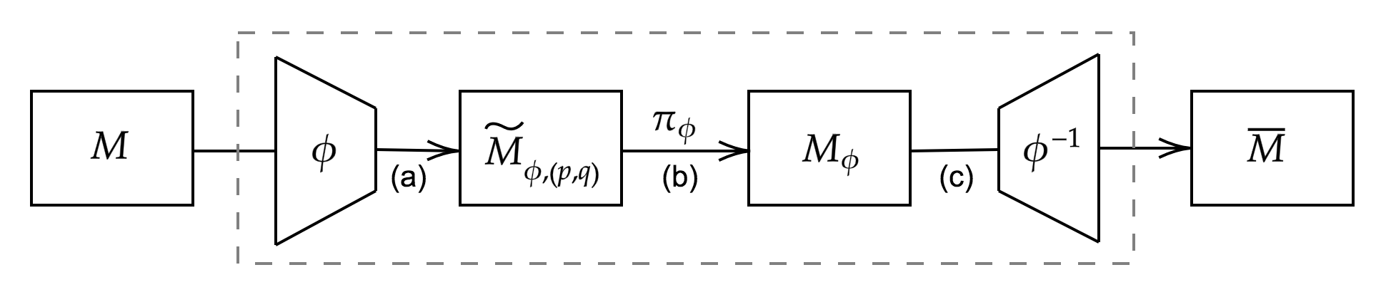
Figure 1: An illustration of our environment shaping framework: it takes the learning environment $M$ as input, and outputs the shaped environment $\overline{M}$. The framework uses an abstraction $\phi$, and a high-level policy $\pi_{\phi}$ as prior knowledge. The steps (a) and (b) of the pipeline are explained in Section 3.2, and step (c) in Section 3.3.

3.1 High-level Ideas

Here, we provide the high-level ideas of our environment shaping framework. Our approach leverages some of the techniques from state abstraction literature [21, 22, 23, 24]. In particular, we rely on compressed knowledge of the learning environment in the form of a high-level near-optimal policy to facilitate the RL agent’s learning process. In contrast to potential-based shaping techniques, which require access to an appropriate potential function such as the exact/approximate optimal value function of the original learning environment, the domain knowledge demanded by our framework is practically feasible to obtain.

To formally explain the key ideas of our abstraction based shaping framework and the domain knowledge required for us, we begin by defining the following notions of approximate abstractions:

Definition 1 ([24, 25]).

Let $\mathcal{X}_{\phi}$ be a finite set. Given an MDP $M=\left({\mathcal{S},\mathcal{A},T,R,\mu_{0},\gamma}\right)$ and state abstraction $\phi:\mathcal{S}\rightarrow\mathcal{X}_{\phi}$, we define three types of abstractions as follows:

1. $\phi$ is $\left({\epsilon_{R},\epsilon_{T}}\right)$-approximate model irrelevant if $\forall{s_{1},s_{2}\in\mathcal{S}}$ where $\phi\left({s_{1}}\right)=\phi\left({s_{2}}\right)$, we have, $\forall{a\in\mathcal{A}}$:

   $$\left|R\left({s_{1},a}\right)-R\left({s_{2},a}\right)\right|\leq\epsilon_{R}\quad\text{and}\quad\sum_{x^{\prime}\in\mathcal{X}_{\phi}}\left|T\left({x^{\prime}\mid s_{1},a}\right)-T\left({x^{\prime}\mid s_{2},a}\right)\right|\leq\epsilon_{T},$$ (5)

   where $T\left({x^{\prime}\mid s,a}\right):=\int_{\mathcal{S}}T\left({s^{\prime}\mid s,a}\right)\mathbf{1}\left\{{\phi\left({s^{\prime}}\right)=x^{\prime}}\right\}ds^{\prime}$ for $x^{\prime}\in\mathcal{X}_{\phi}$, $s\in\mathcal{S}$, and $a\in\mathcal{A}$.

2. $\phi$ is $\epsilon_{Q^{*}}$-approximate $Q^{*}$-irrelevant if there exists an abstract state-action value function $f_{\phi}:\mathcal{X}_{\phi}\times\mathcal{A}\rightarrow\mathbb{R}$ such that the following condition holds:

   $$\sup_{s,a}\left|Q^{*}_{M}\left({s,a}\right)-f_{\phi}\left({\phi\left({s}\right),a}\right)\right|~{}\leq~{}\epsilon_{Q^{*}}.$$ (6)

3. $\phi$ is $\epsilon_{V^{*}}$-approximate $V^{*}$-irrelevant if there exists an abstract policy $\pi_{\phi}:\mathcal{X}_{\phi}\rightarrow\mathcal{A}$ such that the following condition holds:

   $$\sup_{s}\left|V^{*}_{M}\left({s}\right)-V^{\left[{\pi_{\phi}}\right]_{M}}_{M}\left({s}\right)\right|~{}\leq~{}\epsilon_{V^{*}},$$ (7)

   where the lifted policy $\left[{\pi_{\phi}}\right]_{M}:\mathcal{S}\rightarrow\mathcal{A}$ is defined as $\left[{\pi_{\phi}}\right]_{M}\left({s}\right):=\pi_{\phi}\left({\phi\left({s}\right)}\right)$.

Formally, as a prior knowledge, our shaping framework requires access to an $\epsilon_{V^{*}}$-approximate $V^{*}$-irrelevant abstraction $\phi:\mathcal{S}\rightarrow\mathcal{X}_{\phi}$ (where $\mathcal{X}_{\phi}$ is a discrete set), and a corresponding policy $\pi_{\phi}:\mathcal{X}_{\phi}\rightarrow\mathcal{A}$ that satisfies the condition (7). In Section 4, we discuss the ways of obtaining such an abstraction, policy pair $\left({\phi,\pi_{\phi}}\right)$. Given this pair as an input, our abstraction-based shaping framework consists of the following two key steps:

1. First, starting from the tuple $\left({M,\phi,\pi_{\phi}}\right)$, we construct an intermediate MDP $M_{\phi}=\left({\mathcal{X}_{\phi},\mathcal{A},T_{\phi},R_{\phi},\left({\mu_{0}}\right)_{\phi},\gamma}\right)$ such that the policy $\pi_{\phi}$ is the unique optimal policy for $M_{\phi}$. In addition, we ensure that $\pi_{\phi}$ is $\delta$ better than any other policy in the MDP $M_{\phi}$. This step makes our shaping technique fundamentally different from the potential-based shaping methods. We formalize this construction in Section 3.2.

2. Then, using the intermediate MDP $M_{\phi}$, and the abstraction $\phi$, we construct our target MDP $\overline{M}$ such that the mapping $\phi$ is model irrelevant to $\overline{M}$. From this construction, we can show that any $\epsilon_{\mathrm{opt}}$-near optimal policy in $\overline{M}$ is also near optimal in the original MDP $M$. This construction is explained in Section 3.3.

Our overall framework is illustrated in Figure 1.

3.2 Construction of $M_{\phi}$

In this intermediate step, we aim to construct an MDP $M_{\phi}$, defined in the abstract space, that satisfies certain technical conditions formally explained below. These conditions are essential to preserving the optimality behavior between the original learning environment and our final shaped environment. We note that this intermediate step along with these conditions distinguishes our shaping framework from the potential-based shaping methods.

In order to formalize the preferred properties of the MDP $M_{\phi}$, we first introduce some distance measures between the components of the MDP $M_{\phi}$ and the original MDP $M$, for $p,q\geq 0$:

$$D_{p,q}\left({T,{T}_{\phi}}\right)~{}:=~{} \left[{\int_{\mathcal{S}}\sum_{a}\left\{{\left[{\int_{\mathcal{S}}\left|T\left({s^{\prime}\mid s,a}\right)-\frac{{T}_{\phi}\left({\phi\left({s^{\prime}}\right)\mid\phi\left({s}\right),a}\right)}{\int_{\mathcal{S}}\mathbf{1}\left\{{\phi\left({\bar{s}}\right)=\phi\left({s^{\prime}}\right)}\right\}d\bar{s}}\right|^{q}ds^{\prime}}\right]^{\frac{1}{q}}}\right\}^{p}ds}\right]^{\frac{1}{p}},$$

$$D_{p}\left({R,{R}_{\phi}}\right)~{}:=~{} \left[{\int_{\mathcal{S}}\sum_{a}{\left|R\left({s,a}\right)-{R}_{\phi}\left({\phi\left({s}\right),a}\right)\right|}^{p}ds}\right]^{\frac{1}{p}},\text{ and }$$

$$D_{p}\left({\mu_{0},\left({\mu_{0}}\right)_{\phi}}\right)~{}:=~{} \left[{\int_{\mathcal{S}}{\left|\mu_{0}\left({s}\right)-\left({\mu_{0}}\right)_{\phi}\left({\phi\left({s}\right)}\right)\right|}^{p}ds}\right]^{\frac{1}{p}},$$

where ${T}_{\phi}$, ${R}_{\phi}$, and $\left({\mu_{0}}\right)_{\phi}$ belong to the following sets:

$$\mathcal{T}_{\phi}~{}:=~{} \left\{{{T}_{\phi}:\mathcal{X}_{\phi}\times\mathcal{X}_{\phi}\times\mathcal{A}\rightarrow\left[{0,1}\right]\text{ s.t. }{T}_{\phi}\left({\cdot\mid x,a}\right)\in\Delta^{\left|\mathcal{X}_{\phi}\right|},\forall{x\in\mathcal{X}_{\phi},a\in\mathcal{A}}}\right\},$$

$$\mathcal{R}_{\phi}~{}:=~{} \left\{{{R}_{\phi}:\mathcal{X}_{\phi}\times\mathcal{A}\rightarrow\mathbb{R}}\right\},\text{ and }$$

$$\left({\mathcal{P}_{0}}\right)_{\phi}~{}:=~{} \left\{{\left({\mu_{0}}\right)_{\phi}:\mathcal{X}_{\phi}\rightarrow\left[{0,1}\right]\text{ s.t. }\left({\mu_{0}}\right)_{\phi}\left({\cdot}\right)\in\Delta^{\left|\mathcal{X}_{\phi}\right|}}\right\}$$

respectively. Specifically, we are interested in the case where $p\to\infty$, and $q=1$. These distance measures quantify the level of modification done to the original learning environment. Based on the above definitions, we formalize the properties that we seek to ensure while constructing the MDP $M_{\phi}$. Given $\left({M,\phi,\pi_{\phi}}\right)$, we aim to construct a new MDP $M_{\phi}=\left({\mathcal{X}_{\phi},\mathcal{A},T_{\phi},R_{\phi},\left({\mu_{0}}\right)_{\phi},\gamma}\right)$ such that the following conditions holds:

1. $D_{p,q}\left({T,{T}_{\phi}}\right)$, $D_{p}\left({R,{R}_{\phi}}\right)$, and $D_{p}\left({\mu_{0},\left({\mu_{0}}\right)_{\phi}}\right)$ are minimized, i.e., we enforce the new MDP $M_{\phi}$ to not to change too much from the original MDP $M$.

2. $M_{\phi}$ has a unique deterministic optimal policy $\pi^{*}_{M_{\phi}}$, and it satisfies:

   1. $\pi_{\phi}\left({x}\right)=\pi^{*}_{M_{\phi}}\left({x}\right)=\mathop{\rm arg\,max}_{\pi}V^{\pi}_{M_{\phi}}\left({x}\right)$ for all $x\in\mathcal{X}_{\phi}$.

   2. any other deterministic policy in $M_{\phi}$ cannot be $\delta$-near optimal in the following sense:

      $$Q^{*}_{M_{\phi}}\left({x,\pi_{\phi}\left({x}\right)}\right)~{}\geq~{}Q^{*}_{M_{\phi}}\left({x,a^{\prime}}\right)+\delta,\quad\forall{a^{\prime}\neq\pi_{\phi}\left({x}\right),x\in\mathcal{X}_{\phi}}.$$ (8)

Now, we sketch a way of obtaining such an MDP $M_{\phi}$. First, we construct an intermediate MDP ${\widetilde{M}}_{\phi,\left({p,q}\right)}=\left({\mathcal{X}_{\phi},\mathcal{A},T_{\phi,\left({p,q}\right)},R_{\phi,p},\left({\mu_{0}}\right)_{\phi,p},\gamma}\right)$ as follows:

$$T_{\phi,\left({p,q}\right)}~{}\leftarrow~{} \mathop{\rm arg\,min}_{{T}_{\phi}\in\mathcal{T}_{\phi}}D_{p,q}\left({T,{T}_{\phi}}\right),$$

$$R_{\phi,p}~{}\leftarrow~{} \mathop{\rm arg\,min}_{{R}_{\phi}\in\mathcal{R}_{\phi}}D_{p}\left({R,{R}_{\phi}}\right),\text{ and }$$

$$\left({\mu_{0}}\right)_{\phi,p}~{}\leftarrow~{} \mathop{\rm arg\,min}_{\left({\mu_{0}}\right)_{\phi}\in\left({\mathcal{P}_{0}}\right)_{\phi}}D_{p}\left({\mu_{0},\left({\mu_{0}}\right)_{\phi}}\right).$$

After obtaining ${\widetilde{M}}_{\phi,\left({p,q}\right)}$, we can construct our target $M_{\phi}$ by leveraging techniques from [16, 17, 18].

3.3 Construction of $\overline{M}$

Now, we turn to our final step of constructing our target MDP $\overline{M}$, which can be viewed as a decompression step. In this case, we assume that both the reward and the transition dynamics can be modified. Then, given the abstraction $\phi$, and the MDP $M_{\phi}$ constructed in Section 3.2, we construct a shaped MDP $\overline{M}=\left({\mathcal{S},\mathcal{A},\overline{T},\overline{R},\overline{\mu}_{0},\gamma}\right)$ as follows:

1. $\overline{T}\left({s^{\prime}\mid s,a}\right)=\frac{T_{\phi}\left({\phi\left({s^{\prime}}\right)\mid\phi\left({s}\right),a}\right)}{\int_{\mathcal{S}}\mathbf{1}\left\{{\phi\left({\tilde{s}}\right)=\phi\left({s^{\prime}}\right)}\right\}d\tilde{s}}$, for all $s^{\prime}\in\mathcal{S},s\in\mathcal{S},a\in\mathcal{A}$

2. $\overline{R}\left({s,a}\right)=R_{\phi}\left({\phi\left({s}\right),a}\right)$, for all $s\in\mathcal{S},a\in\mathcal{A}$

3. $\overline{\mu}_{0}\left({s}\right)=\left({\mu_{0}}\right)_{\phi}\left({\phi\left({s}\right)}\right)$, for all $s\in\mathcal{S}$

Finally, we want to ensure that our teaching objective, mentioned in Section 2, can be attained by this shaped environment $\overline{M}$. To this end, the following theorem shows that the agent’s policy learnt in the shaped environment $\overline{M}$ preserves near-optimal behavior in the original environment $M$. Then, in Section 5, we empirically demonstrate that our shaping framework indeed helps in accelerating the learning process of the RL agent.

Theorem 1.

Any $\epsilon_{\mathrm{opt}}$-near optimal policy $\pi_{\overline{M}}:\mathcal{S}\rightarrow\Delta\left({\mathcal{A}}\right)$ of $\overline{M}$, satisfies the following condition:

$$\sup_{s}\left|V^{*}_{M}\left({s}\right)-V^{\pi_{\overline{M}}}_{M}\left({s}\right)\right|~{}\leq~{}\epsilon^{\prime}_{\mathrm{opt}}~{}:=~{}\epsilon_{V^{*}}+\frac{R_{\mathrm{max}}}{1-\gamma}\cdot\frac{\epsilon_{\mathrm{opt}}}{\delta}.$$ (9)

When $\epsilon_{V^{*}}\leq\frac{R_{\mathrm{max}}}{1-\gamma}\cdot\frac{\epsilon_{\mathrm{opt}}}{\delta}$, we attain our teaching objective Eq. (4) with $c=\frac{R_{\mathrm{max}}}{1-\gamma}\cdot\frac{2}{\delta}$.

Proof.

For the target MDP $\overline{M}$, we first show that $\left[{\pi_{\phi}}\right]_{\overline{M}}$ is the unique optimal policy. One can easily observe that, by construction, $\phi$ is a model-irrelevant abstraction for $\overline{M}$ ($\epsilon_{R}=0$, and $\epsilon_{T}=0$ in Eq. (5)). Then, from Lemma 1 (in the Appendix of the supplementary material), $\phi$ is also a $Q^{*}$-irrelevant abstraction for $\overline{M}$ ($\epsilon_{Q^{*}}=0$ in Eq. (6)), i.e., we have

$$Q^{*}_{\overline{M}}\left({s,a}\right)~{}=~{}Q^{*}_{M_{\phi}}\left({\phi\left({s}\right),a}\right),\forall{s\in\mathcal{S},a\in\mathcal{A}}.$$

And since $\pi_{\phi}$ is the unique optimal policy derived from $Q^{*}_{M_{\phi}}$, we can conclude that $\left[{\pi_{\phi}}\right]_{\overline{M}}$ is the unique optimal policy for $\overline{M}$.

In addition, using the Lemma 5 (in the Appendix of the supplementary material), we can show that any $\epsilon_{\mathrm{opt}}$-near optimal policy $\pi_{\overline{M}}:\mathcal{S}\rightarrow\Delta\left({\mathcal{A}}\right)$ of $\overline{M}$, satisfies the following condition:

$$\sup_{s}\left\lVert\pi_{\overline{M}}\left({\cdot\mid s}\right)-\left[{\pi_{\phi}}\right]_{\overline{M}}\left({\cdot\mid s}\right)\right\rVert_{1}~{}\leq~{}\frac{\epsilon_{\mathrm{opt}}}{\delta}.$$ (10)

Finally, consider:

$$\sup_{s}\left|V^{*}_{M}\left({s}\right)-V^{\pi_{\overline{M}}}_{M}\left({s}\right)\right|~{}\stackrel{{\scriptstyle(i)}}{{=}}~{} \sup_{s}\left|V^{*}_{M}\left({s}\right)-V^{\left[{\pi_{\phi}}\right]_{M}}_{M}\left({s}\right)+V^{\left[{\pi_{\phi}}\right]_{\overline{M}}}_{M}\left({s}\right)-V^{\pi_{\overline{M}}}_{M}\left({s}\right)\right|$$

$$~{}\stackrel{{\scriptstyle(ii)}}{{\leq}}~{} \sup_{s}\left|V^{*}_{M}\left({s}\right)-V^{\left[{\pi_{\phi}}\right]_{M}}_{M}\left({s}\right)\right|+\sup_{s}\left|V^{\left[{\pi_{\phi}}\right]_{\overline{M}}}_{M}\left({s}\right)-V^{\pi_{\overline{M}}}_{M}\left({s}\right)\right|$$

$$~{}\stackrel{{\scriptstyle(iii)}}{{\leq}}~{} \epsilon_{V^{*}}+\sup_{s}\left|V^{\left[{\pi_{\phi}}\right]_{\overline{M}}}_{M}\left({s}\right)-V^{\pi_{\overline{M}}}_{M}\left({s}\right)\right|$$

$$~{}\stackrel{{\scriptstyle(iv)}}{{\leq}}~{} \epsilon_{V^{*}}+\frac{R_{\mathrm{max}}}{1-\gamma}\sup_{s}\left\lVert\pi_{\overline{M}}\left({\cdot\mid s}\right)-\left[{\pi_{\phi}}\right]_{\overline{M}}\left({\cdot\mid s}\right)\right\rVert_{1}$$

$$~{}\stackrel{{\scriptstyle(v)}}{{\leq}}~{} \epsilon_{V^{*}}+\frac{R_{\mathrm{max}}}{1-\gamma}\cdot\frac{\epsilon_{\mathrm{opt}}}{\delta}~{}=~{}\epsilon^{\prime}_{\mathrm{opt}},$$

where $(i)$ is due to the fact that $\left[{\pi_{\phi}}\right]_{\overline{M}}=\left[{\pi_{\phi}}\right]_{M}$, $(ii)$ is by triangle inequality, $(iii)$ is from Eq. (7), $(iv)$ is due to Lemma 2 (in the Appendix of the supplementary material), and $(v)$ is by Eq. (10). ∎

4 Practical Considerations

In this section, we discuss some practical aspects of our environment shaping framework.

Constructing Abstractions.

Here, we briefly discuss the ways of obtaining the abstraction, and high-level policy pair $\left({\phi,\pi_{\phi}}\right)$, which is required as a prior knowledge to our shaping framework. One way of obtaining such knowledge is via careful feature engineering with the help of a domain expert. For example, when the ground state space is raw pixels acquired through noisy sensors, an expert can focus only on the relevant information that is required for the decision making task. One can also utilize the existing computational approaches, such as [26, 27, 28], to automatically construct meaningful abstractions.

Reward-only Shaping.

In the case of shaping via only modifying the reward function, the shaped MDP $\overline{M}$ differs from the original MDP $M$ only in its reward function $R$. In particular, given the abstraction $\phi$, and the MDP $M_{\phi}$ constructed in Section 3.2, we construct a reward-only shaped MDP $\widehat{M}=\left({\mathcal{S},\mathcal{A},\widehat{T},\widehat{R},\widehat{\mu}_{0},\gamma}\right)$ as follows:

1. $\widehat{T}\left({s^{\prime}\mid s,a}\right)={T}\left({s^{\prime}\mid s,a}\right)$, and $\widehat{\mu}_{0}\left({s}\right)=\mu\left({s}\right)$, for all $s^{\prime}\in\mathcal{S},s\in\mathcal{S},a\in\mathcal{A}$

2. $\widehat{R}\left({s,a}\right)=R_{\phi}\left({\phi\left({s}\right),a}\right)$, for all $s\in\mathcal{S},a\in\mathcal{A}$

The following theorem, similar to Theorem 1, provides a guarantee on preserving the optimality behavior in the reward-only shaped environment.

Theorem 2.

We assume the following:

$$\sup_{s,a}~{}\left\lVert T\left({\cdot\mid s,a}\right)-\overline{T}\left({\cdot\mid s,a}\right)\right\rVert_{1}~{}\leq~{}\beta_{T}.$$

Then, any $\epsilon_{\mathrm{opt}}$-near optimal policy $\pi_{\widehat{M}}:\mathcal{S}\rightarrow\Delta\left({\mathcal{A}}\right)$ of $\widehat{M}$, satisfies the following condition:

$$\sup_{s}\left|V^{*}_{M}\left({s}\right)-V^{\pi_{\widehat{M}}}_{M}\left({s}\right)\right|~{}\leq~{}\epsilon_{V^{*}}+\frac{R_{\mathrm{max}}}{1-\gamma}\cdot\frac{1}{\delta}\cdot\left\{{\frac{2\cdot\gamma\cdot\beta_{T}\cdot R_{\phi}^{\mathrm{max}}}{\left({1-\gamma}\right)^{2}}+\epsilon_{\mathrm{opt}}}\right\},$$ (11)

where $R_{\phi}^{\mathrm{max}}=\max_{x,a}\left|R_{\phi}\left({x,a}\right)\right|$.

Transition Dynamics-only Shaping.

Here, we shape only the transition dynamics while keeping the reward function of the shaped MDP $\overline{M}$ is the same as that of the original MDP $M$. In particular, given the abstraction $\phi$, and the MDP $M_{\phi}$ constructed in Section 3.2, we construct a target/shaped MDP $\widehat{M}=\left({\mathcal{S},\mathcal{A},\widehat{T},\widehat{R},\widehat{\mu}_{0},\gamma}\right)$ as follows:

1. $\widehat{T}\left({s^{\prime}\mid s,a}\right)=\frac{T_{\phi}\left({\phi\left({s^{\prime}}\right)\mid\phi\left({s}\right),a}\right)}{\int_{\mathcal{S}}\mathbf{1}\left\{{\phi\left({\tilde{s}}\right)=\phi\left({s^{\prime}}\right)}\right\}d\tilde{s}}$, for all $s^{\prime}\in\mathcal{S},s\in\mathcal{S},a\in\mathcal{A}$

2. $\widehat{R}\left({s,a}\right)=R\left({s,a}\right)$, and $\widehat{\mu}_{0}\left({s}\right)=\mu\left({s}\right)$, for all $s\in\mathcal{S},a\in\mathcal{A}$

The following theorem, similar to Theorem 1, provides a guarantee on preserving the optimality behavior in the dynamics-only shaped environment.

Theorem 3.

We assume the following:

$$\sup_{s,a}~{}\left|R\left({s,a}\right)-\overline{R}\left({s,a}\right)\right|~{}\leq~{}\beta_{R}\cdot\max\left\{{R_{\mathrm{max}},R_{\phi}^{\mathrm{max}}}\right\}.$$

Then, any $\epsilon_{\mathrm{opt}}$-near optimal policy $\pi_{\widehat{M}}:\mathcal{S}\rightarrow\Delta\left({\mathcal{A}}\right)$ of $\widehat{M}$, satisfies the following condition:

$$\sup_{s}\left|V^{*}_{M}\left({s}\right)-V^{\pi_{\widehat{M}}}_{M}\left({s}\right)\right|~{}\leq~{}\epsilon_{V^{*}}+\frac{R_{\mathrm{max}}}{1-\gamma}\cdot\frac{1}{\delta}\cdot\left\{{\frac{2\cdot\beta_{R}\cdot\max\left\{{R_{\mathrm{max}},R_{\phi}^{\mathrm{max}}}\right\}}{{1-\gamma}}+\epsilon_{\mathrm{opt}}}\right\},$$ (12)

where $R_{\phi}^{\mathrm{max}}=\max_{x,a}\left|R_{\phi}\left({x,a}\right)\right|$.

The proofs of Theorems 2 and 3 can be found in the Appendix of the supplementary material.

5 Experimental Evaluation

In this section, we empirically investigate whether our environment shaping approach enables simple reinforcement learning algorithm such as policy gradient, to find (near-)optimal policy under challenging setting with noisy and sparse feedback.

5.1 Environment Details

We consider the object gathering game environment, inspired by environments considered in recent works [29, 30, 31, 32], see Figure 2(a). In this game, an agent starts from one of the corner cells. The goal of the agent is to collect the objects, so that to maximize its total return. By collecting a “star" object, the agent receives a reward of $1.0$, a “plus" object provides $0.04$ reward, and collecting a “dot" object provides either $0.1$ or $-0.1$ reward with equal probability. At initialization, the “star" object always appears opposite corner of the agent’s position, “plus" appears in the four cells distance from the agent’s initial position, and “dot" appears uniformly at random anywhere. After collecting the “plus" object, it appears on the same location, and “dot" object disappears after collecting it. The game’s episode ends when the maximum time step $H=30$ is reached, or the agent has collected the “star" object. In this game we have two actions {“left", “right"}, i.e., $|\mathcal{A}|=2$. The state of the system is represented by the position of the agent and the positions of all three objects. Since we have the number of the cells to be $15$ and our state representation is described as the concatenation of the binary vector of the position of the agent and the position of each object, it will give us rise to $15^{4}$ total possible states, i.e., $|\mathcal{S}|=15^{4}$. The transition dynamics of the environment is defined as follows: with probability $0.99$, the actions succeed in navigating the agent to left or right, as shown with the arrows in Figure 2(a); and with probability $0.01$, the move to the opposite direction is performed. The rewards are discounted at $\gamma=0.99$. The optimal policy $\pi^{*}$ is to go towards to the “star" object and collect it.

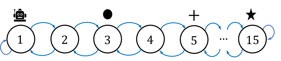
(a) Environment

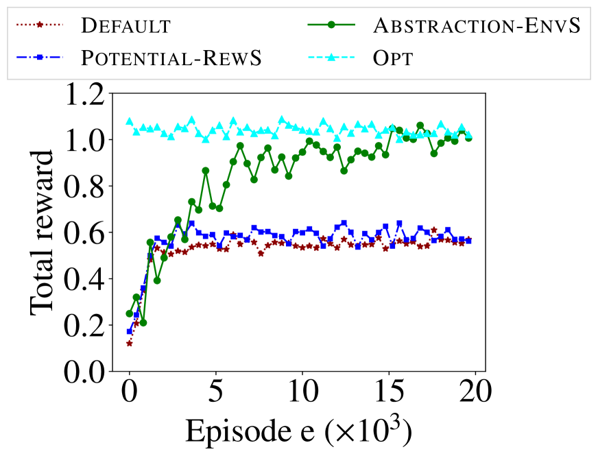
(b) Performance

Figure 2: (a) An example of the gathering game environment with the actions $\mathcal{A}$={"left", "right"} and the state space size $|\mathcal{S}|=15^{4}$. (b) Learning curves for gathering game task, averaged across 30 runs of each algorithm with random initialization.

5.2 Experimental Setup

We use the vanilla policy gradient method as the agent’s algorithm, where the policy network is implemented as a two-layer neural network with relu activation function and softmax on the last layer. A one-hot vector of length $15$, corresponding to the number of cells, represents the agent’s location and the positions of all three objects in the environment. Hence the length of the input vector to the neural network is $4\times 15=60$.

Methods evaluated. The following algorithms were considered in the comparison: (i) default baseline with training on original $M$ (Default), (ii) baseline of potential-based reward shaping of $M$ (Potential-RewS) (see [6]), (iii) training on $\overline{M}$ shaped using our approach (Abstraction-EnvS), and (iv) optimal policy that follows object “star" (Opt).

For the Potential-RewS approach, we need to approximate the optimal value function $V_{M}^{*}$ of the original MDP $M$. To this end, we first run the policy gradient algorithm up to $50,000$ iterations, and then used resulting policy $\pi$ to approximate $V_{M}^{*}$ by $V_{M}^{\pi}$. To estimate the value function of the policy $\pi$, we used Monte Carlo (MC) prediction algorithm with $100,000$ samples. Given that we have domain knowledge of our problem, e.g., the information about the agent’s position and ‘star" object’s position is sufficient to learn the optimal behavior, our abstraction $\phi:\mathcal{S}\rightarrow\mathcal{X}_{\phi}$ can be defined as follows: we consider only the position of the agent and position of the “star" object to encode our state space. This abstraction reduces the state-space from $15^{4}$ down to $15^{2}$, i.e., $|\mathcal{X}_{\phi}|=15^{2}$. We construct the MDP $M_{\phi}$ by first obtaining ${\widetilde{M}}_{\phi,\left({2,1}\right)}$ and then using the rewards only attack as in [17].

5.3 Results

We evaluate the performance of the four algorithms mentioned above and report the results by averaging across $30$ runs and with random initialization for each run. Figure 2(b) shows the convergence of the total reward of the episode for all the algorithms, where the policy following the “star" object attains the optimal value. As expected, training on the shaped environment outperforms two baselines.

Since the training on the original environment $M$ needs exponentially many episodes to learn optimal policy, it converges to a local minimum [33], e.g., collecting the nearest object “plus". Since our environment provides noisy signals feedback because of the randomness of the “dot" object, it is challenging to compute an appropriate potential function. As a result, the applicability of the potential-based reward shaping is limited in our settings.

6 Conclusions

In this work, we propose an abstraction based environment shaping framework to accelerate the learning process of an agent. Our framework is fundamentally different from the existing potential-based shaping methods. We theoretically prove that our environment shaping preserves the optimality behavior between the original and target MDPs, and empirically demonstrate its efficacy on tasks with sparse and noisy feedback signals.

Appendix A Auxiliary Lemmas

Lemma 1 (Theorem 2 from [25]).

If $\phi$ is an $\left({\epsilon_{R},\epsilon_{T}}\right)$-approximate model-irrelevant abstraction, then $\phi$ is also an approximate $Q^{*}$-irrelevant abstraction with approximation error $\epsilon_{Q^{*}}=\frac{\epsilon_{R}}{1-\gamma}+\frac{\gamma\epsilon_{T}R_{\mathrm{max}}}{2\left({1-\gamma}\right)^{2}}$. Further, if $\phi$ is an $\epsilon_{Q^{*}}$-approximate $Q^{*}$-irrelevant abstraction, then $\phi$ is also an approximate $V^{*}$-irrelevant abstraction with approximation error $\epsilon_{V^{*}}=\frac{2\epsilon_{Q^{*}}}{1-\gamma}$.

Lemma 2 (Lemma A.1 from [34]).

For any two policy $\pi$ and $\pi^{\prime}$ (acting in the MDP $M$), we have

$$\sup_{s}\left|V^{\pi}_{M}\left({s}\right)-V^{\pi^{\prime}}_{M}\left({s}\right)\right|~{}\leq~{}\frac{R_{\mathrm{max}}}{1-\gamma}\sup_{s}\left\lVert\pi\left({\cdot\mid s}\right)-\pi^{\prime}\left({\cdot\mid s}\right)\right\rVert_{1}.$$

Definition 2 (approximately-equivalent MDPs, adapted from [35]).

Suppose we have two MDPs $M_{1}=\left({\mathcal{S},\mathcal{A},T_{1},R_{1},\left({\mu_{0}}\right)_{1},\gamma}\right)$ and $M_{2}=\left({\mathcal{S},\mathcal{A},T_{2},R_{2},\left({\mu_{0}}\right)_{2},\gamma}\right)$, and rewards are bounded in $\left[{0,R_{\mathrm{max}}}\right]$. We call $M_{1}$ and $M_{2}$ as $\left({\beta_{R},\beta_{T}}\right)$ approximately-equivalent if the following holds:

$$\sup_{s\in\mathcal{S},a\in\mathcal{A}}~{}\left|R_{1}\left({s,a}\right)-R_{2}\left({s,a}\right)\right|~{}\leq~{} \beta_{R}\cdot R_{\mathrm{max}}$$

$$\sup_{s\in\mathcal{S},a\in\mathcal{A}}~{}\left\lVert T_{1}\left({\cdot\mid s,a}\right)-T_{2}\left({\cdot\mid s,a}\right)\right\rVert_{1}~{}\leq~{} \beta_{T}.$$

Lemma 3.

Suppose we have two $\left({\beta_{R},\beta_{T}}\right)$ approximately-equivalent MDPs $M_{1}$ and $M_{2}$. Then, we have:

$$\sup_{s}\left|V^{*}_{M_{1}}\left({s}\right)-V^{*}_{M_{2}}\left({s}\right)\right|~{}\leq~{}\frac{\beta_{R}\cdot R_{\mathrm{max}}}{1-\gamma}+\frac{\gamma\cdot\beta_{T}\cdot R_{\mathrm{max}}}{\left({1-\gamma}\right)^{2}}.$$

Proof.

Consider the Bellman optimality equation, for any $s$:

$$V^{*}_{M}(s)~{}=~{}\max_{a}Q^{*}_{M}(s,a)~{}=~{}\max_{a}\left\{{R(s,a)+\gamma\int_{\mathcal{S}}T(s^{\prime}\mid s,a)V^{*}_{M}(s^{\prime})ds^{\prime}}\right\}$$

Then, for any $s$, we have:

$$\left|V^{*}_{M_{1}}(s)-V^{*}_{M_{2}}(s)\right|$$

$$=~{} \left|\max_{a}Q^{*}_{M_{1}}(s,a)-\max_{a^{\prime}}Q^{*}_{M_{2}}(s,a^{\prime})\right|$$

$$\leq~{} \max_{a}\left|Q^{*}_{M_{1}}(s,a)-Q^{*}_{M_{2}}(s,a)\right|$$

$$=~{} \max_{a}\left|{\mathbf{s}}{R_{1}(s,a)-R_{2}(s,a)}+\gamma\int_{\mathcal{S}}{\mathbf{s}}{T_{1}(s^{\prime}\mid s,a)V^{*}_{M_{1}}(s^{\prime})-T_{2}(s^{\prime}\mid s,a)V^{*}_{M_{2}}(s^{\prime})}ds^{\prime}\right|$$

$$\leq~{} \max_{a}\left|R_{1}(s,a)-R_{2}(s,a)\right|+\gamma\max_{a}\left|\int_{\mathcal{S}}{\mathbf{s}}{T_{1}(s^{\prime}\mid s,a)V^{*}_{M_{1}}(s^{\prime})-T_{2}(s^{\prime}\mid s,a)V^{*}_{M_{2}}(s^{\prime})}ds^{\prime}\right|$$

$$\leq~{} \beta_{R}\cdot R_{\mathrm{max}}+\gamma\max_{a}\left|\int_{\mathcal{S}}{\mathbf{s}}{T_{1}(s^{\prime}\mid s,a)-T_{2}(s^{\prime}\mid s,a)}V^{*}_{M_{1}}(s^{\prime})ds^{\prime}-\int_{\mathcal{S}}T_{2}(s^{\prime}\mid s,a){\mathbf{s}}{V^{*}_{M_{2}}(s^{\prime})-V^{*}_{M_{1}}(s^{\prime})}ds^{\prime}\right|$$

$$\leq~{} \beta_{R}\cdot R_{\mathrm{max}}+\gamma\max_{a}\left\{{\left|\int_{\mathcal{S}}{\mathbf{s}}{T_{1}(s^{\prime}\mid s,a)-T_{2}(s^{\prime}\mid s,a)}V^{*}_{M_{1}}(s^{\prime})ds^{\prime}\right|+\left|\int_{\mathcal{S}}T_{2}(s^{\prime}\mid s,a){\mathbf{s}}{V^{*}_{M_{2}}(s^{\prime})-V^{*}_{M_{1}}(s^{\prime})}ds^{\prime}\right|}\right\}$$

$$\leq~{} \beta_{R}\cdot R_{\mathrm{max}}+\gamma\max_{a}\left\{{\left\lVert T_{1}(\cdot\mid s,a)-T_{2}(\cdot\mid s,a)\right\rVert_{1}\sup_{s^{\prime}}V^{*}_{M_{1}}(s^{\prime})+\left\lVert T_{2}(\cdot\mid s,a)\right\rVert_{1}\sup_{s^{\prime}}\left|V^{*}_{M_{1}}(s^{\prime})-V^{*}_{M_{2}}(s^{\prime})\right|}\right\}$$

$$\leq~{} \beta_{R}\cdot R_{\mathrm{max}}+\gamma\max_{a}\left\{{\left\lVert T_{1}(\cdot\mid s,a)-T_{2}(\cdot\mid s,a)\right\rVert_{1}\frac{R_{\mathrm{max}}}{1-\gamma}+1\cdot\sup_{s^{\prime}}\left|V^{*}_{M_{1}}(s^{\prime})-V^{*}_{M_{2}}(s^{\prime})\right|}\right\}$$

$$\leq~{} \beta_{R}\cdot R_{\mathrm{max}}+\frac{\gamma\cdot\beta_{T}\cdot R_{\mathrm{max}}}{1-\gamma}+\gamma\sup_{s^{\prime}}\left|V^{*}_{M_{1}}(s^{\prime})-V^{*}_{M_{2}}(s^{\prime})\right|$$

Taking sup over $s$, and rearranging the terms complete the proof. ∎

Lemma 4 (adapted from [35]).

Suppose we have two $\left({\beta_{R},\beta_{T}}\right)$ approximately-equivalent MDPs $M_{1}$ and $M_{2}$. Then for any policy $\pi:\mathcal{S}\rightarrow\Delta\left({\mathcal{A}}\right)$, we have:

$$\sup_{s}\left|V^{\pi}_{M_{1}}\left({s}\right)-V^{\pi}_{M_{2}}\left({s}\right)\right|~{}\leq~{}\frac{\beta_{R}\cdot R_{\mathrm{max}}}{1-\gamma}+\frac{\gamma\cdot\beta_{T}\cdot R_{\mathrm{max}}}{\left({1-\gamma}\right)^{2}}.$$

Lemma 5.

Consider an MDP $M=\left({\mathcal{S},\mathcal{A},T,R,P_{0},\gamma}\right)$ with a unique deterministic optimal policy $\pi^{*}_{M}:\mathcal{S}\rightarrow\mathcal{A}$ such that the following holds:

$$V^{*}_{M}\left({s}\right)~{}=~{}Q^{*}_{M}\left({s,\pi^{*}_{M}\left({s}\right)}\right)~{}\geq~{}Q^{*}_{M}\left({s,a^{\prime}}\right)+\delta,\quad\forall{a^{\prime}\neq\pi^{*}_{M}\left({s}\right),s\in\mathcal{S}}.$$ (13)

Then any $\epsilon_{\mathrm{opt}}$-near optimal policy $\pi:\mathcal{S}\rightarrow\Delta\left({\mathcal{A}}\right)$ for $M$ (as given in (3)) satisfies the following:

$$\sup_{s}\left\lVert\pi^{*}_{{M}}\left({\cdot\mid s}\right)-\pi\left({\cdot\mid s}\right)\right\rVert_{1}~{}\leq~{}\frac{\epsilon_{\mathrm{opt}}}{\delta}.$$

Further, any other deterministic policy $\pi:\mathcal{S}\rightarrow\mathcal{A}$ cannot be $\epsilon_{\mathrm{opt}}$-near optimal when $\epsilon_{\mathrm{opt}}<\delta$.

Proof.

Denote $f\left({s,\pi\left({s}\right)}\right)=\mathbb{E}_{a\sim\pi\left({\cdot\mid s}\right)}\!\left[f\left({s,a}\right)\right]$. First, we note that for any $s\in\mathcal{S}$, we have

$$Q^{*}_{M}\left({s,\pi\left({s}\right)}\right)~{}\geq~{}Q^{\pi}_{M}\left({s,\pi\left({s}\right)}\right)~{}=~{}V^{\pi}_{M}\left({s}\right).$$ (14)

Fix any state $s\in\mathcal{S}$. Let $a_{s}^{*}=\pi^{*}_{M}\left({s}\right)$, $a^{\prime}_{s}$ be one of the second best action after $a^{*}_{s}$, and $p=\pi\left({a_{s}^{*}\mid s}\right)$. Then, we have

$$Q^{*}_{M}\left({s,\pi\left({s}\right)}\right)~{}=~{} \mathbb{E}_{a\sim\pi\left({\cdot\mid s}\right)}\!\left[R\left({s,a}\right)+\mathbb{E}_{s^{\prime}\sim T\left({\cdot\mid s,a}\right)}\!\left[V^{*}_{M}\left({s^{\prime}}\right)\right]\right]$$

$$~{}\leq~{} p\cdot Q^{*}_{M}\left({s,a_{s}^{*}}\right)+\overline{p}\cdot Q^{*}_{M}\left({s,a^{\prime}_{s}}\right),$$ (15)

where $\bar{p}=1-p$. Consider

$$\overline{p}\cdot\delta~{}\stackrel{{\scriptstyle(i)}}{{\leq}}~{} \overline{p}\cdot\left\{{Q^{*}_{M}\left({s,a_{s}^{*}}\right)-Q^{*}_{M}\left({s,a^{\prime}_{s}}\right)}\right\}$$

$$~{}\stackrel{{\scriptstyle(ii)}}{{\leq}}~{} Q^{*}_{M}\left({s,a_{s}^{*}}\right)-Q^{*}_{M}\left({s,\pi\left({s}\right)}\right)$$

$$~{}\stackrel{{\scriptstyle(iii)}}{{\leq}}~{} V^{*}_{M}\left({s}\right)-V^{\pi}_{M}\left({s}\right)$$

$$~{}\leq~{} \epsilon_{\mathrm{opt}}.$$

where $(i)$, $(ii)$, and $(iii)$ are due to Eqs. (13), (15), and (14) respectively. Thus, we get

$$\left\lVert\pi^{*}_{{M}}\left({\cdot\mid s}\right)-\pi\left({\cdot\mid s}\right)\right\rVert_{1}~{}=~{}\overline{p}~{}\leq~{}\frac{\epsilon_{\mathrm{opt}}}{\delta}.$$

When $\epsilon_{\mathrm{opt}}<\delta$ and $\pi$ is deterministic s.t. $\pi\neq\pi^{*}_{M}$, from Eqs. (13), and (14), we have:

$$V^{*}_{M}\left({s}\right)~{}\geq~{}V^{\pi}_{M}\left({s}\right)+\delta~{}>~{}V^{\pi}_{M}\left({s}\right)+\epsilon_{\mathrm{opt}}.$$

∎

Proof of Theorem 2.

Proof.

Note that $\widehat{M}$ and $\overline{M}$ are $\left({0,\beta_{T}}\right)$ approximately-equivalent. We first show that $\pi_{\widehat{M}}$ is near-optimal in $\overline{M}$, then using Theorem 1 completes the proof. For any $s\in\mathcal{S}$, we have:

$$\left|V^{*}_{\overline{M}}\left({s}\right)-V^{\pi_{\widehat{M}}}_{\overline{M}}\left({s}\right)\right|$$

$$~{}\leq~{} \left|V^{*}_{\overline{M}}\left({s}\right)-V^{*}_{\widehat{M}}\left({s}\right)\right|+\left|V^{*}_{\widehat{M}}\left({s}\right)-V^{\pi_{\widehat{M}}}_{\widehat{M}}\left({s}\right)\right|+\left|V^{\pi_{\widehat{M}}}_{\widehat{M}}\left({s}\right)-V^{\pi_{\widehat{M}}}_{\overline{M}}\left({s}\right)\right|$$

$$~{}\leq~{} \frac{\gamma\cdot\beta_{T}\cdot R_{\phi}^{\mathrm{max}}}{\left({1-\gamma}\right)^{2}}+\epsilon_{\mathrm{opt}}+\frac{\gamma\cdot\beta_{T}\cdot R_{\phi}^{\mathrm{max}}}{\left({1-\gamma}\right)^{2}},$$

where the last inequality is due to Lemma 3 and Lemma 4. ∎

Proof of Theorem 3.

Proof.

Note that $\widehat{M}$ and $\overline{M}$ are $\left({\beta_{R},0}\right)$ approximately-equivalent. We first show that $\pi_{\widehat{M}}$ is near-optimal in $\overline{M}$, then using Theorem 1 completes the proof. For any $s\in\mathcal{S}$, we have:

$$\left|V^{*}_{\overline{M}}\left({s}\right)-V^{\pi_{\widehat{M}}}_{\overline{M}}\left({s}\right)\right|$$

$$~{}\leq~{} \left|V^{*}_{\overline{M}}\left({s}\right)-V^{*}_{\widehat{M}}\left({s}\right)\right|+\left|V^{*}_{\widehat{M}}\left({s}\right)-V^{\pi_{\widehat{M}}}_{\widehat{M}}\left({s}\right)\right|+\left|V^{\pi_{\widehat{M}}}_{\widehat{M}}\left({s}\right)-V^{\pi_{\widehat{M}}}_{\overline{M}}\left({s}\right)\right|$$

$$~{}\leq~{} \frac{\beta_{R}\cdot\max\left\{{R_{\mathrm{max}},R_{\phi}^{\mathrm{max}}}\right\}}{{1-\gamma}}+\epsilon_{\mathrm{opt}}+\frac{\beta_{R}\cdot\max\left\{{R_{\mathrm{max}},R_{\phi}^{\mathrm{max}}}\right\}}{{1-\gamma}},$$

where the last inequality is due to Lemma 3 and Lemma 4. ∎

Appendix B Additional Experiments

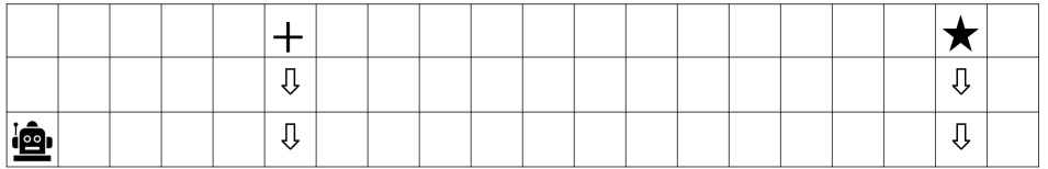
(a) Environment

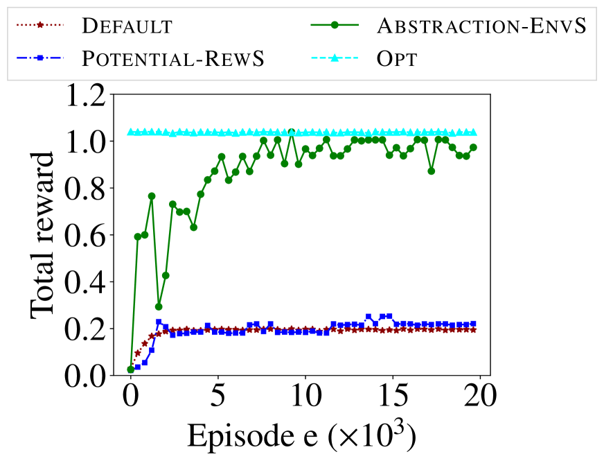
(b) Performance

Figure 3: (a) An example of the catcher environment with the actions $\mathcal{A}$={"left", "right"} and the state space size $|\mathcal{S}|=20\times 60^{2}$. (b) Learning curves for catcher task, averaged across 30 runs.

In this section, we performed an additional experiment to showcase the efficacy of our algorithm.

B.1 Environment Details

We consider the catcher environment illustrated in Figure 3(a). In this game, an agent moves along the x-axis, and two types of objects fall from above the agent, perpendicular to the agent’s axis of movement. In this game, the agent has two actions, i.e., $\mathcal{A}$={“left", “right"}. The action taken succeeds in moving the agent in the corresponding direction with a probability of $0.99$. And with a probability of $0.01$, the movement happens in the opposite direction. The agent starts from the left corner of the environment, and its goal is to move itself to catch the falling objects. The object “plus" always appears close to the agent’s initial position, e.g., on the $5^{\mathrm{th}}$ column, and the object “star" appears before the last column. Intersecting with the object “star" gives the reward of $1.0$, and intersecting with the object “plus" gives the reward of $0.04$. After catching or missing the objects, they appear in the starting position. The game’s episode ends when the maximum time step $H=30$ is reached, or the agent has caught the “star" object. Since we have the number of the cells to be $60$ and our state representation is described as the concatenation of the binary vector of the position of the agent and the locations of each object, it results in $20\times 60^{2}$ total possible states, i.e., $|\mathcal{S}|=20\times 60^{2}$. The rewards are discounted at $\gamma=0.99$. The optimal policy $\pi^{*}$ is to catch the “star" object.

B.2 Experimental Setup

We use the vanilla policy gradient method as the agent’s algorithm, where the policy network is implemented as a two-layer neural network with relu activation function and softmax on the last layer. A one-hot vector of length $20$, corresponding to the number of cells in the x-axis, represents the agent’s location. One-hot vectors of length $60$, corresponding to the number of cells, represent the positions of all two objects in the environment. Hence the length of the input vector to the neural network is $20+2\times 60=140$.

Methods evaluated.

As in Section 5, the following algorithms were considered in the comparison: (i) default baseline with training on original $M$ (Default), (ii) baseline of potential-based reward shaping of $M$ (Potential-RewS) (see [6]), (iii) training on $\overline{M}$ shaped using our approach (Abstraction-EnvS), and (iv) optimal policy that catches object “star" (Opt).

For the Potential-RewS approach, we need to approximate the optimal value function $V_{M}^{*}$ of the original MDP $M$. To this end, we first run the policy gradient algorithm up to $50,000$ iterations, and then used resulting policy $\pi$ to approximate $V_{M}^{*}$ by $V_{M}^{\pi}$. To estimate the value function of the policy $\pi$, we used Monte Carlo (MC) prediction algorithm with $200,000$ samples. Given that we have domain knowledge of our problem, e.g., the information about the agent’s position and “star" object’s position is sufficient to learn the optimal behavior, our abstraction $\phi:\mathcal{S}\rightarrow\mathcal{X}_{\phi}$ can be defined as follows: we consider only the position of the agent and position of the “star" object to encode our state space. This abstraction reduces the state-space from $20\times 60^{2}$ down to $20\times 60$, i.e., $|\mathcal{X}_{\phi}|=20\times 60$. We construct the MDP $M_{\phi}$ by first obtaining ${\widetilde{M}}_{\phi,\left({2,1}\right)}$ and then using the rewards only attack as in [17].

We evaluate the performance of the four algorithms mentioned above and report the results by averaging across $30$ runs and with random initialization for each run (cf., Figure 3(b)).

References

- [1] Richard S Sutton, David A McAllester, Satinder P Singh, and Yishay Mansour. Policy gradient methods for reinforcement learning with function approximation. In Advances in neural information processing systems, pages 1057–1063, 2000.
- [2] Richard S Sutton and Andrew G Barto. Reinforcement learning: An introduction. MIT press, 2018.
- [3] Volodymyr Mnih, Koray Kavukcuoglu, David Silver, Andrei A Rusu, Joel Veness, Marc G Bellemare, Alex Graves, Martin Riedmiller, Andreas K Fidjeland, Georg Ostrovski, et al. Human-level control through deep reinforcement learning. Nature, 518(7540):529–533, 2015.
- [4] David Silver, Julian Schrittwieser, Karen Simonyan, Ioannis Antonoglou, Aja Huang, Arthur Guez, Thomas Hubert, Lucas Baker, Matthew Lai, Adrian Bolton, et al. Mastering the game of go without human knowledge. Nature, 550(7676):354–359, 2017.
- [5] Timothy P Lillicrap, Jonathan J Hunt, Alexander Pritzel, Nicolas Heess, Tom Erez, Yuval Tassa, David Silver, and Daan Wierstra. Continuous control with deep reinforcement learning. arXiv preprint arXiv:1509.02971, 2015.
- [6] Andrew Y Ng, Daishi Harada, and Stuart Russell. Policy invariance under reward transformations: Theory and application to reward shaping. In ICML, volume 99, pages 278–287, 1999.
- [7] Jette Randløv. Shaping in reinforcement learning by changing the physics of the problem. In ICML, pages 767–774. Citeseer, 2000.
- [8] Daniel S Brown and Scott Niekum. Machine teaching for inverse reinforcement learning: Algorithms and applications. In Proceedings of the AAAI Conference on Artificial Intelligence, volume 33, pages 7749–7758, 2019.
- [9] Luis Haug, Sebastian Tschiatschek, and Adish Singla. Teaching inverse reinforcement learners via features and demonstrations. In Advances in Neural Information Processing Systems, pages 8464–8473, 2018.
- [10] Parameswaran Kamalaruban, Rati Devidze, Volkan Cevher, and Adish Singla. Interactive teaching algorithms for inverse reinforcement learning. In IJCAI, pages 2692–2700, 2019.
- [11] Marco Colombetti and Marco Dorigo. Training agents to perform sequential behavior. Adaptive behavior, 2(3):247–275, 1994.
- [12] Maja J Mataric. Reward functions for accelerated learning. In Machine Learning Proceedings 1994, pages 181–189. Elsevier, 1994.
- [13] Eric Wiewiora. Potential-based shaping and q-value initialization are equivalent. Journal of Artificial Intelligence Research, 19:205–208, 2003.
- [14] Sam Michael Devlin and Daniel Kudenko. Dynamic potential-based reward shaping. In Proceedings of the 11th International Conference on Autonomous Agents and Multiagent Systems, pages 433–440. IFAAMAS, 2012.
- [15] John Asmuth, Michael L Littman, and Robert Zinkov. Potential-based shaping in model-based reinforcement learning. In AAAI, pages 604–609, 2008.
- [16] Yuzhe Ma, Xuezhou Zhang, Wen Sun, and Jerry Zhu. Policy poisoning in batch reinforcement learning and control. In Advances in Neural Information Processing Systems, pages 14543–14553, 2019.
- [17] Amin Rakhsha, Goran Radanovic, Rati Devidze, Xiaojin Zhu, and Adish Singla. Policy teaching via environment poisoning: Training-time adversarial attacks against reinforcement learning. In ICML, 2020.
- [18] Xuezhou Zhang, Yuzhe Ma, Adish Singla, and Xiaojin Zhu. Adaptive reward-poisoning attacks against reinforcement learning. In ICML, 2020.
- [19] Haoqi Zhang and David C Parkes. Value-based policy teaching with active indirect elicitation. In AAAI, volume 8, pages 208–214, 2008.
- [20] Martin L Puterman. Markov decision processes: discrete stochastic dynamic programming. John Wiley & Sons, 2014.
- [21] Robert Givan, Thomas Dean, and Matthew Greig. Equivalence notions and model minimization in markov decision processes. Artificial Intelligence, 147(1-2):163–223, 2003.
- [22] Balaraman Ravindran and Andrew G Barto. Approximate homomorphisms: A framework for non-exact minimization in markov decision processes. 2004.
- [23] Lihong Li, Thomas J Walsh, and Michael L Littman. Towards a unified theory of state abstraction for mdps. In ISAIM, 2006.
- [24] David Abel, David Hershkowitz, and Michael Littman. Near optimal behavior via approximate state abstraction. In International Conference on Machine Learning, pages 2915–2923, 2016.
- [25] Nan Jiang. Notes on state abstractions, 2019. URL: http://nanjiang.cs.illinois.edu/files/cs598/note4.pdf. Last visited on 2020/05/05.
- [26] Nicholas K Jong and Peter Stone. State abstraction discovery from irrelevant state variables. In IJCAI, volume 8, pages 752–757, 2005.
- [27] David Abel, Dilip Arumugam, Kavosh Asadi, Yuu Jinnai, Michael L Littman, and Lawson LS Wong. State abstraction as compression in apprenticeship learning. In Proceedings of the AAAI Conference on Artificial Intelligence, volume 33, pages 3134–3142, 2019.
- [28] Sean R. Sinclair, Siddhartha Banerjee, and Christina Lee Yu. Adaptive discretization for episodic reinforcement learning in metric spaces. POMACS, 2019.
- [29] Joel Z. Leibo, Vinícius Flores Zambaldi, Marc Lanctot, Janusz Marecki, and Thore Graepel. Multi-agent reinforcement learning in sequential social dilemmas. In AAMAS, pages 464–473, 2017.
- [30] Roberta Raileanu, Emily Denton, Arthur Szlam, and Rob Fergus. Modeling others using oneself in multi-agent reinforcement learning. In ICML, pages 4254–4263, 2018.
- [31] A. Ghosh, S. Tschiatschek, H. Mahdavi, and A. Singla. Towards deployment of robust cooperative ai agents: An algorithmic framework for learning adaptive policies. In AAMAS, 2020.
- [32] Sebastian Tschiatschek, Ahana Ghosh, Luis Haug, Rati Devidze, and Adish Singla. Learner-aware teaching: Inverse reinforcement learning with preferences and constraints. In Advances in Neural Information Processing Systems, 2019.
- [33] Sham M. Kakade and John Langford. Approximately optimal approximate reinforcement learning. In ICML, 2002.
- [34] Wen Sun, Geoffrey J Gordon, Byron Boots, and J Bagnell. Dual policy iteration. In Advances in Neural Information Processing Systems, pages 7059–7069, 2018.
- [35] Eyal Even-Dar and Yishay Mansour. Approximate equivalence of markov decision processes. In Learning Theory and Kernel Machines, pages 581–594. Springer, 2003.