Lithium in the context of Multiple Populations in Globular Clusters

Abstract

Multiple Populations represent the standard for Globular Clusters (GC): a fraction (10–50%) of their stars have the same elemental abundances of halo stars of similar metallicity (first generation, or 1G), but the other stars (second generation, 2G) are characterised by patterns of light elements abundances which resemble those typical of gas processed by proton–capture reactions at high temperature. Consequently, we should naively expect that Lithium is destroyed in the 2G stars, but instead it is generally observed, at abundances only slightly depleted with respect to the 1G stars. After discussing the models for the formation of multiple populations, I examine the role of dilution with pristine gas and the possible role of the Asymptotic Giant Branch (AGB) scenario in accounting for the Lithium patterns in GC stars. Super–AGB and AGB yields of Lithium, produced by the Cameron Fowler mechanism in the ‘Hot Bottom Burning’ convective envelopes, may help to explain the peculiar high Lithium in a few extreme 2G stars. On the other hand, modeling the abundances in mild 2G stars depends explicitly on whether the initial Li in the gas forming the 1G stars and the diluting gas of the 2G ones is that predicted by the Big Bang nucleosynthesis or the $\sim$3 times smaller value observed at the surface of halo dwarfs.

1 Introduction

There are two scientific problems which are interconnected, when we study the Lithium patterns in the multiple populations (MPops) of GCs.
The first one is of special interest to this meeting on ‘Lithium in the Universe’ and it is: how can we solve the problem of the discrepancy between the Li abundance predicted by the standard Big–Bang cosmology (e.g. Pitrou et al., 2018) and the observations of the Li abundance at the surface of warm population II stars, which is a factor 2–3 smaller (see Fig. 1 and its references)? Many researchers agree that the reason behind this discrepancy is ‘simply’ due to stellar depletion mechanisms acting at the surface of these stars, and this point of view is supported by the fact that the lowest metallicity stars ([Fe/H]$<$–2.5) indeed show smaller Li, with a larger star–to–star spread, than the remarkably similar value $\log\epsilon$(Li)$\sim 2.2-2.3$ of the warm dwarfs at $-2.5<$ [Fe/H] $<-1.5$, suggesting a variation in the effect of the depletion mechanisms due to the physical changes in the structure of the lowest metallicity stars. In addition, models by Richard et al. (2005), are plausibly in agreement both with the plateau and with the depletion of Li at [Fe/H]$<$–2.5.
The second problem is: how were the GC stars showing composition ‘anomalies’ formed, and is Lithium a key tool to choose a formation model?

2 Multiple populations

GCs display a a great number of signatures that reveal the presence of multiple populations (MPops). While one population (in general a minority of the cluster stars) has a chemical tagging similar to field halo stars, and therefore is called “first generation” (1G), the other stars have chemical abundances of “light” elements typical of gas processed at high temperature by proton capture reactions (including ⁴He) and are globally dubbed “second generation” or 2G. The signatures are found by many different observation tools:

1) high dispersion spectroscopy reveals that the abundance patterns of light elements display “anticorrelations”, the most relevant of which is the Na vs. O anticorrelation. Anticorrelated are also Mg and Al and Si and Mg, in the (more restricted) number of clusters in which Mg variations are clearly detected (see for a summary Gratton et al., 2019);

2) traditional photometry in optical or near IR bands has shown the presence of multiple main sequences in a few clusters, indicating populations with different helium abundance Bedin et al. (2004); Piotto et al. (2007);

3) HST UV spectrophotometry showed that the UV bands F275W and F336W powerfully magnify N (and C and O) abundance differences in the spectra (Piotto et al., 2015). Thus “chromosome maps”, diagrams in two pseudo-colors, were built in which the 1G and different groups of 2G occupy different regions (Milone et al., 2017). Chromosome maps allowed to extend to large stellar samples the results of high dispersion spectroscopy, and clearly showed the ubiquity, variety and discreteness of MPops (Renzini et al., 2015). For a comparison between high dispersion results and chromosome maps see Marino et al. (2019).

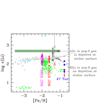
Figure 1: Compilation of data and model results discussed in this talk. In the plane $log\epsilon$(Li) vs. [Fe/H] we plot some reference data for the Globular Clusters: NGC 6397 from Lind et al. (2009), NGC 6752 from Shen et al. (2010), 47 Tuc from Bonifacio et al. (2007) plus the limits by D’Orazi et al. (2010), included in the interval limited by the red line and upper limit. The red giant data from $\omega\,{\rm{Cen}}$ by Mucciarelli et al. (2018) are plotted as small green crosses, with a big green cross indicating the location of the peculiar giant #25664 (Mucciarelli et al., 2019). The $\omega\,{\rm{Cen}}$ points are scaled up by 1 dex to include the approximate dilution factor at the first dredge up. The halo subdwarfs data are from Meléndez et al. (2010) (analysis by non-LTE models, grey triangles) and Sbordone et al. (2010) (cyan squares). At [Fe/H]=–1.3 and –1.4 we plot the abundances in the ejecta of AGB models (4–6$\,{M}_{\odot}$: red circles) and super-AGB models (6.5–7.5$\,{M}_{\odot}$: black light circles, the 7.5$\,{M}_{\odot}$ is out of scale) by Ventura & D’Antona (2010) and the super–AGB yields by Di Criscienzo et al. (2018); D’Antona et al. (2019) (6.5-7.5$\,{M}_{\odot}$, heavy black circles). The dashed green upper band represents the Big–Bang Lithium abundance, while the lower dash–dotted lines represent the average Li at the surface of halo stars. The two possible interpretations for the initial lithium in the gas forming the 1G GC stars, and for the gas diluting the ejecta in the 2G stars are shown as case A and B.

3 The AGB scenario

If a model has to deal with the observed abundance patterns, it must, first of all, identify a (stellar) source of gas processed by p–captures at high or very high temperature and then explain how the formation of 2G stars occurs in this gas. We refer the reader to the review by Gratton et al. (2019) for a description of the models, and here we limit ourselves to say that the MPops, in GCs where Mg is depleted, are only compatible with the “supermassive” stars (SMS) scenario (Denissenkov & Hartwick, 2014), maybe in the excretion-belt version by Gieles et al. (2018), and the AGB scenario (D’Ercole et al., 2008). In this latter model, the p–captures occur at the bottom of the very hot convective envelopes of luminous massive AGBs (“hot bottom burning”, HBB), the winds lost by these stars at low velocity collect in a cooling flow at the center of the GC, where they can form 2G stars, either from the ‘pure’ ejecta, or from the ejecta diluted with re–accreted pristine gas. The AGB scenario has been explored both from the nucleosynthesis of AGBs point of view (Ventura & D’Antona, 2009; Ventura et al., 2011; Ventura et al., 2013; Ventura et al., 2018), from the dynamical point of view (D’Ercole et al., 2008, 2016; Bekki, 2011; Calura et al., 2019) and for its consequences on the long term evolution of the spatial distribution of the two stellar generations (e.g. Vesperini et al., 2010, 2011, 2013)

The SMS scenario would be favoured as it predicts more correctly the Mg isotopes ratios in the 2G, but Ventura et al. (2018) have shown that a reasonable change in the cross section of ²⁵Mg+p and ²⁶Mg+p rates in the temperature region of interest ($100-120$MK) can produce agreement also for the AGB scenario. On the other hand, the SMS scenario has the drawback that no SMS has ever been observed, and it does not explain why Mg depletion is more significant in metal poor GCs, a peculiarity well explained in the AGB scenario (Ventura et al., 2011).
Is Lithium the key element to choose between the two models?

4 Lithium patterns and the MPops

The role of Lithium is indeed very simple. If high temperature p-captures are needed to explain the abundance patterns, these same p-captures have already destroyed ⁷Li at a much lower temperature inside the evolving star! Nevertheless, ⁷Li is present in 2G stars, as shown by many observations (for a complete summary, see Gratton et al., 2019).

This conundrum has two possible tentative solutions:

1) the gas from which the 2G stars were born is diluted with standard pop. II gas, which has preserved the starting abundance. In fact, the typical O–Na, Mg–Al anticorrelations are explained by dilution of ejecta (O-poor, Na-rich, Mg-poor, Al-rich…) with standard pop. II gas. Most clusters display a Na–Li anticorrelation too, which can be the signature of dilution of 2G matter, Na rich but Li-free, with matter having standard Na and Li (e.g. Decressin et al., 2007). On the other hand, Gratton et al. (2019) stress that the dilution factors inferred from the observations and the Li in 2G stars require that the ejecta can not be Li–poor.

2) In the AGB scenario, the same HBB which is responsible for the anomalous composition of the 2G stars, also produces fresh lithium by the Cameron & Fowler (1971) mechanism. Li remains at very high abundances in the envelope until ³He is totally consumed, and eventually it is fully burned. Thus the massive AGBs can expel Li with the gas lost during their initial HBB phase, and contribute to the Li abundance of the mixture.

A problem with this hypothesis is that the Li average abundance in the ejecta is scarcely constrained, due to its strong dependence on the mass-loss rate during the lithium rich phase (see the still actual discussion in Ventura & D’Antona, 2005).

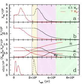
Figure 2: Surface abundances of Li, O, Mg and Na along the evolution of super–AGBs of masses 6.5, and 7 M_⊙, from Di Criscienzo et al. (2018); D’Antona et al. (2019). Different regions of HBB re highlighted for the 6.5$\,{M}_{\odot}$: 1st (yellow): region of Li–production by the Cameron-Fowler mechanism and Na production by burning of the Ne obtained by the second dredge up; 2nd (pink): Na destruction, O and Mg depletion, Al formation; 3rd (green): Si production and steady decrease in Al.

5 The peculiar Li–rich 2G stars: in NGC 2808 and $\omega\,{\rm{Cen}}$

Figure 2 shows the time evolution of light elements in the envelopes of super–AGB stars of 6.5 and 7$\,{M}_{\odot}$(Di Criscienzo et al., 2018). Along the evolution, the stellar luminosity increases and the HBB temperature $T\rm_{HBB}$ increases too, favoring more extreme p-captures. So, Li is formed as soon as the star climbs along the AGB, even before the second dredge up is finished ($T\rm_{HBB}$$\sim$40 MK), and also Na reaches its largest abundances, due to the second dredge up and the p-captures on the dredged up ²²Ne. Later on (when $T\rm_{HBB}$$>$65 MK) the NO cycle becomes efficient and Oxygen declines, while the Mg-Al chain becomes efficient too. In the latest phases, Si builds up (and Al begins declining). The elemental yields therefore come from very different physical conditions ($T\rm_{HBB}$) and Li and extreme p-processed gas can coexist.

The AGB scenario also predicts that the “extreme” population —the group whose helium abundance is at the highest values— present in some GCs was formed from pure AGB/super–AGB gas (D’Ercole et al., 2008; D’Antona et al., 2016). Thus the elemental abundance in these stars should reflect directly the composition of the ejecta.

Among several giants observed by D’Orazi et al. (2015) in the GC NGC 2808, one (#46518) belongs to the “extreme” population and its Li is a bare factor of two smaller than in the 1G giants of the same sample. Note that D’Orazi et al. (2015) consider in the same class all the giants having a similarly high Al abundance, but actually we have seen in Fig. 2 that Al can be reduced when Si is produced, so Al is a very general indicator of 2G, and not an indicator of the most extreme stars only. On the contrary, the location of #46518 in the chromosome map shows that it has indeed the most extreme composition (Marino et al., 2019). In D’Antona et al. (2019) we show that the abundances in the #46518 giant are compatible with its direct birth of super-AGB ejecta, while its Li abundance requires a large degree of dilution with pristine, Li-rich, gas, if this star was born in the SMS scenario.

An extreme case is that of the $\omega\,{\rm{Cen}}$ giant with extreme Li and Na abundances discovered by Mucciarelli et al. (2019). The star is shown in Fig. 1 as the green cross at the top. It may be compatible with the abundances in the most extreme super-AGB ejecta computed by Ventura & D’Antona (2010), and easily explained by looking at Fig. 2: in fact the maximum abundance of Li and Na in the envelopes of super–AGBs (and massive AGBs) occur at the same time. Therefore, if mass loss occurs mainly at this epoch, as in the most massive super–AGBs, we will find very high Li and Na in the ejecta. Note that a measure of other abundances in these giants may disprove this interpretation: we do not expect extremely low O and Mg, nor high Al in this star.

Thus, when the Li observed abundance is very large, in the context of the AGB scenario, we should find a direct correlation between Li and Na abundance. In all other cases, we expect to find an anticorrelation (as found), which can be attributed to dilution.

6 Which Li in pristine diluting gas?

A deceiving point which can be overlooked when considering the role of Li abundance in the ejecta is related to how we interpret the abundances at the surface of pop. II dwarfs. This is illustrated in Fig. 1, where the Li Big Bang abundance (see, e.g. Pitrou et al., 2018) is shown by the dashed green band at the top, and the average dwarf location is within the two dash-dotted lines. We can take two different points of view:

(A) the abundance in the gas forming the 1G is the Big Bang abundance, and stellar depletion mechanisms bring it down to the value at the surface of dwarfs;

(B) the abundance in the gas forming the 1G is that seen at the surface of dwarfs.

If the ejecta have no Li it is unimportant if the lower abundance at the surface is already in the gas or it is achieved later on at the stellar surface, and case (A) or (B) give the same result for any mixture. But if the diluting gas has a finite Li abundance as in the AGB ejecta, and similar processes at the stellar surface deplete Li in both 1G and 2G stars, in case (A) the gas abundance resulting from a mixture of pristine and AGB gas will result in a smaller abundance than in case (B). If we want to obtain a particular Li abundance at the surface of a 2G dwarf, in case (A), the Li abundance in the ejecta, for a given degree of dilution with pristine gas, must be a factor $\sim$2.5 larger than in case (B). In the simplest exaample, a mild 2G dwarf, for which we have estimated a dilution factor is $\sim$0.5, shows a standard pop.II abundance $\log\epsilon$(Li)=2.3. If we want to obtain this abundance in case B, we need that both the 50% pristine gas and the 50% AGB gas have $\log\epsilon$(Li)=2.3. But in case A we need that both have $\log\epsilon$(Li)=2.7 (then depleted at the surface). Thus Li in the ejecta of all AGB forming the 2G should be close to the Big Bang abundance, values which are found in today’s models only from the high tail of super–AGB masses (see Fig. 1). A plausible solution to this problem is achieved if the dilution factors for 2G stars (e.g. given in Gratton et al. (2019)) have been underestimated.

7 Conclusions

The Lithium observations in GC stars are a powerful tool to investigate their MPops, and the abundances in the 2G stars may favour or help to dismiss the different formation models. We find that only exceptional extreme stars of the 2G, such as the candidates discussed here in NGC 2808 and $\omega\,{\rm{Cen}}$ directly favour the AGB scenario, while the mild 2G stars having only mildly depleted Li abundances may be consistent with a scenario in which the ejecta (of any model) are strongly diluted.
Nevertheless, if the AGB scenario will be recognized as the best model for MPops, we will get a totally independent hint of the reliability of the Big Bang abundance.

References

- Bedin et al. (2004) Bedin L. R., Piotto G., Anderson J., Cassisi S., King I. R., Momany Y., Carraro G., 2004, ApJ, 605, L125
- Bekki (2011) Bekki K., 2011, MNRAS, 412, 2241
- Bonifacio et al. (2007) Bonifacio P., et al., 2007, A&A, 470, 153
- Calura et al. (2019) Calura F., D’Ercole A., Vesperini E., Vanzella E., Sollima A., 2019, MNRAS, 489, 3269
- Cameron & Fowler (1971) Cameron A. G. W., Fowler W. A., 1971, ApJ, 164, 111
- D’Antona (1991) D’Antona F., 1991, Mem. Soc. Astron. Italiana, 62, 1
- D’Antona et al. (2016) D’Antona F., Vesperini E., D’Ercole A., Ventura P., Milone A. P., Marino A. F., Tailo M., 2016, MNRAS, 458, 2122
- D’Antona et al. (2019) D’Antona F., Ventura P., Fabiola Marino A., Milone A. P., Tailo M., Di Criscienzo M., Vesperini E., 2019, ApJ, 871, L19
- D’Ercole et al. (2008) D’Ercole A., Vesperini E., D’Antona F., McMillan S. L. W., Recchi S., 2008, MNRAS, 391, 825
- D’Ercole et al. (2016) D’Ercole A., D’Antona F., Vesperini E., 2016, MNRAS, 461, 4088
- D’Orazi et al. (2010) D’Orazi V., Lucatello S., Gratton R., Bragaglia A., Carretta E., Shen Z., Zaggia S., 2010, ApJ, 713, L1
- D’Orazi et al. (2015) D’Orazi V., et al., 2015, MNRAS, 449, 4038
- Decressin et al. (2007) Decressin T., Charbonnel C., Meynet G., 2007, A&A, 475, 859
- Denissenkov & Hartwick (2014) Denissenkov P. A., Hartwick F. D. A., 2014, MNRAS, 437, L21
- Di Criscienzo et al. (2018) Di Criscienzo M., Ventura P., D’Antona F., Dell’Agli F., Tailo M., 2018, MNRAS, 479, 5325
- Gieles et al. (2018) Gieles M., et al., 2018, MNRAS, 478, 2461
- Gratton et al. (2019) Gratton R., Bragaglia A., Carretta E., D’Orazi V., Lucatello S., Sollima A., 2019, A&A Rev., 27, 8
- Lind et al. (2009) Lind K., Primas F., Charbonnel C., Grundahl F., Asplund M., 2009, A&A, 503, 545
- Marino et al. (2019) Marino A. F., et al., 2019, MNRAS, 487, 3815
- Meléndez et al. (2010) Meléndez J., Casagrande L., Ramírez I., Asplund M., Schuster W. J., 2010, A&A, 515, L3
- Michaud & Richer (1991) Michaud G., Richer J., 1991, Mem. Soc. Astron. Italiana, 62, 151
- Milone et al. (2017) Milone A. P., et al., 2017, MNRAS, 464, 3636
- Mucciarelli et al. (2018) Mucciarelli A., Salaris M., Monaco L., Bonifacio P., Fu X., Villanova S., 2018, A&A, 618, A134
- Mucciarelli et al. (2019) Mucciarelli A., Monaco L., Bonifacio P., Salaris M., Fu X., Villanova S., 2019, A&A, 623, A55
- Piotto et al. (2007) Piotto G., et al., 2007, ApJ, 661, L53
- Piotto et al. (2015) Piotto G., et al., 2015, AJ, 149, 91
- Pitrou et al. (2018) Pitrou C., Coc A., Uzan J.-P., Vangioni E., 2018, Phys. Rep., 754, 1
- Renzini et al. (2015) Renzini A., et al., 2015, MNRAS, 454, 4197
- Richard et al. (2005) Richard O., Michaud G., Richer J., 2005, ApJ, 619, 538
- Sbordone et al. (2010) Sbordone L., et al., 2010, A&A, 522, A26
- Shen et al. (2010) Shen Z. X., Bonifacio P., Pasquini L., Zaggia S., 2010, A&A, 524, L2
- Ventura & D’Antona (2005) Ventura P., D’Antona F., 2005, A&A, 439, 1075
- Ventura & D’Antona (2009) Ventura P., D’Antona F., 2009, A&A, 499, 835
- Ventura & D’Antona (2010) Ventura P., D’Antona F., 2010, MNRAS, 402, L72
- Ventura et al. (2011) Ventura P., Carini R., D’Antona F., 2011, MNRAS, 415, 3865
- Ventura et al. (2013) Ventura P., Di Criscienzo M., Carini R., D’Antona F., 2013, MNRAS, 431, 3642
- Ventura et al. (2018) Ventura P., D’Antona F., Imbriani G., Di Criscienzo M., Dell’Agli F., Tailo M., 2018, MNRAS, 477, 438
- Vesperini et al. (2010) Vesperini E., McMillan S. L. W., D’Antona F., D’Ercole A., 2010, ApJ, 718, L112
- Vesperini et al. (2011) Vesperini E., McMillan S. L. W., D’Antona F., D’Ercole A., 2011, MNRAS, 416, 355
- Vesperini et al. (2013) Vesperini E., McMillan S. L. W., D’Antona F., D’Ercole A., 2013, MNRAS, 429, 1913