An entropy structure preserving space-time formulation for cross-diffusion systems: analysis and Galerkin discretization

Abstract

Cross-diffusion systems are systems of nonlinear parabolic partial differential equations that are used to describe dynamical processes in several application, including chemical concentrations and cell biology. We present a space-time approach to the proof of existence of bounded weak solutions of cross-diffusion systems, making use of the system entropy to examine long-term behavior and to show that the solution is nonnegative, even when a maximum principle is not available. This approach naturally gives rise to a novel space-time Galerkin method for the numerical approximation of cross-diffusion systems that conserves their entropy structure. We prove existence and convergence of the discrete solutions, and present numerical results for the porous medium, the Fisher-KPP, and the Maxwell-Stefan problem.

35K51, 35K55, 35Q92, 65M60, 41A10

1 Introduction

In this paper we develop a new space-time approach to the celebrated boundedness by entropy method by Ansgar Jüngel [26]. For a textbook version see [27]; see also [31, 11].

Cross-diffusion systems are systems of nonlinear parabolic partial differential equations that are commonly used to describe dynamical processes appearing in modeling, for example, population dynamics, ion transport through nanopores, tumor growth models, and multicomponent gas mixtures. The challenge in the analysis of these systems is that the diffusion matrix is not necessarily symmetric nor positive semi-definite, and thus no maximum principle is available. Following [26], the remedy is to make use of the entropy structure of the system. Introducing the entropy function, a transformation of the solution, allows us to examine long-term behavior and show that the solution is nonnegative and bounded. Here, we present a space-time approach to the proof of existence of bounded weak solutions of cross-diffusion systems. The main tool will be the method of compensated compactness, which is a special technique of applying the classical div-curl lemma [48]. The key difference to the existing literature is that we do not make use of time-stepping, but instead consider time and space altogether. This naturally leads to a novel space-time Galerkin method for the numerical approximation of cross-diffusion systems. The space-time approach entails test and trail spaces, as well as the mesh, where time is included as additional dimension. This provides an easy way to increase the approximation degree simultaneously in space and time, and makes space-time $hp$-refinement possible. In a schematic way, our overall approach consists of the following four steps:

1. space-time variational formulation,

2. transformation to entropy variables,

3. regularization with a space-time $H^{1}$ inner product,

4. Galerkin discretization.

Existing numerical schemes for cross-diffusion systems rely on time-stepping methods. An entropy/energy conserving time-stepping algorithm for thermomechanical problems was developed in [41] being of second order in time. In [32], assuming existence of sufficient regular strong solutions on some time interval $[0,T]$ of a scalar diffusion equation, Runge-Kutta methods were studied using maximal regularity. Although maximal regularity also applies to a certain type of cross-diffusion systems [42], Runge-Kutta methods were only applied to very restrictive classes; an example (semi-discrete Runge-Kutta scheme) can be found in [29]. In [25], an entropy diminishing/mass conserving fully discrete variational formulation for a cross-diffusion system was presented. An alternative discretization for cross-diffusion systems based on the change to entropy-variables has been proposed in [16], where a dissipation-preserving approximation by Galerkin methods in space and discontinuous Galerkin methods in time has beed studied.

Maxwell-Stefan systems, see [46, 37], describe multicomponent diffusive fluxes in non-dilute solutions or gas mixtures, and are a prime example for the cross-diffusion systems considered here. The first result on global solutions for the Maxwell-Stefan equations close to the equilibrium is given in [23]. The global existence of solutions close to equilibrium and the large time convergence to this equilibrium can be found in [21, Chapter 9], [22, 24], and [42, Chapter 12]. The proof of existence of local classical solutions to the Maxwell-Stefan equations can be found in [6]. For a textbook on this topic, see [42]. The fact that the Maxwell-Stefan equations satisfy the assumptions made in this paper, see (H1)-(H3) below, is due to [30], where the entropy structure of the Maxwell-Stefan system was used to prove the existence of globally bounded weak solutions. An entropy structure was also identified for a generalized Maxwell-Stefan system coupled to the Poisson equation in [28], where the existence of global weak solutions was proven as well. The unconditional convergence to the unique equilibrium for given mass was shown in [24, 36] without reaction terms. Those results were extended to also include reaction terms using mass-action kinetics in [13], whenever a detailed balance equilibrium exists. The heat equation can be recovered from the Maxwell-Stefan equation as a relaxation limit [43].

As of yet, numerical schemes for the Maxwell-Stefan equations commonly employ time-stepping. A finite differences approximation can be found in [34, 35]. Fast solvers for explicit finite-difference schemes were studied in [20]. A posteriori estimates for finite elements in the stationary case are given in [10]. In [40], a mass conserving finite volume scheme was presented. Existence of solutions for a mixed finite element scheme under some restrictions on the coefficients was proven in [38]. The scheme of [14] was proven to also conserve the $L^{\infty}$ bound by making use of a maximum principle. A scheme using finite elements in space and implicit Euler in time was used to approximate a Poisson-Maxwell-Stefan system in [28]. That scheme, which is based on a formulation in entropy variables, admits solutions that conserve the mass as well as the entropy structure. As a by product, the solution satisfy an $L^{\infty}$ bound. Another scheme that is mass conserving and conserves the $L^{\infty}$ bounds of the solutions was presented in [8].

On simultaneous space-time finite element approaches for parabolic problems, there is a rich literature on the linear case, focusing on the heat equation; see, e.g. the recent overview [33, Ch. 7]. We point out that due to the different orders of derivatives present, conforming discretizations are typically based on a Petrov-Galerkin approach; see e.g. [4, 45, 2, 47, 50]. For nonlinear parabolic equations, the existing literature on space-time methods is much sparser. The adaptive finite element scheme introduced in [17] for linear parabolic problems was extended in [18] to the scalar version of the nonlinear reaction-diffusion equation treated in this paper. A space-time discontinuous Galerkin method for scalar nonlinear convection and diffusion was introduced in [49]. A space-time method for nonlinear PDEs using adaptive wavelets was introduced in [1].

The structure of this paper is as follows. In Section 2, we state the problem and make the necessary assumptions for the existence of an entropy function. In Section 3, we present the space-time Galerkin method on a regularized formulation of the problem in the entropy variable unknown, and state our two main results in Proposition 3.3 and Proposition 3.4, namely existence and convergence of discrete solutions, respectively. Existence of discrete solutions is proven in Section 3.1. The proof of convergence will be split into two parts, first showing convergence with respect to mesh size in Section 3.2, then proving convergence as the regularization parameter goes to zero in Section 3.3. In Section 3.4, we are then able to prove existence of a weak solution of the continuous problem. Numerical tests for the porous medium, the Fisher-KPP, and the Maxwell-Stefan problem are presented in Section 4. All numerical results were obtained using the finite element software NGSolve, see [44]. Additionally, in Section 5, we reformulate the Maxwell-Stefan system with implicitly given currents in terms of the concentrations, and test it numerically.

2 General setting

Let $\Omega\subset\mathbb{R}^{d}$ be a bounded domain, and $\rho_{0}\in L^{\infty}(\Omega)^{N}$, $N\geq 1$, a vector-valued function. We consider the following nonlinear reaction-diffusion system in the vector-valued unknown $\rho(t)=(\rho_{1},\ldots,\rho_{N})(\cdot,t):\Omega\to\mathbb{R}^{N}$:

(1) $$\begin{cases}\partial_{t}\rho-\nabla\cdot(A(\rho)\nabla\rho)=f(\rho)&\mbox{in }\Omega,\ t>0,\\ (A(\rho)\nabla\rho)\cdot\nu=0&\mbox{on }\partial\Omega,\ t>0,\\ \rho(0)=\rho_{0}&\mbox{in }\Omega.\end{cases}$$

Here, $A(\rho)\in\mathbb{R}^{N\times N}$ is the diffusion matrix, $f(\rho):\mathbb{R}^{N}\to\mathbb{R}^{N}$ represents the reactions, and $\nu$ is the outward pointing unit normal vector at $\partial\Omega$; moreover, for $1\leq i\leq N$,

$$\left(\nabla\cdot(A(\rho)\nabla\rho)\right)_{i}=\sum_{\mu=1}^{d}\sum_{j=1}^{N}\frac{\partial}{\partial x_{\mu}}\left(A_{ij}(\rho)\frac{\partial\rho_{j}}{\partial x_{\mu}}\right),\quad\left((A(\rho)\nabla\rho)\cdot\nu\right)_{i}=\sum_{\mu=1}^{d}\sum_{j=1}^{N}A_{ij}(\rho)\frac{\partial\rho_{j}}{\partial x_{\mu}}\nu_{\mu}.$$

We make the following hypotheses, which are slightly stronger assumptions compared to those made by A. Jüngel in [26].

1. $A\in C^{0}(\overline{\mathcal{D}};\mathbb{R}^{N\times N})$ and $f\in C^{0}(\overline{\mathcal{D}};\mathbb{R}^{N})$, for a bounded domain $\mathcal{D}\subset(0,\infty)^{N}$.

2. There exists a convex function $s\in C^{2}(\mathcal{D},[0,\infty))\cap C^{0}(\overline{\mathcal{D}})$, with $s^{\prime}:\mathcal{D}\to\mathbb{R}^{N}$ invertible and $u:=(s^{\prime})^{-1}\in C^{1}(\mathbb{R}^{N},\mathcal{D})$, such that the following two conditions are satisfied:

   1. There exists a constant $\gamma>0$ such that

      $$\ z\cdot s^{\prime\prime}(\rho)A(\rho)z\geq\gamma|z|^{2}\qquad\forall z\in\mathbb{R}^{N},\,\rho\in\mathcal{D}.$$

      Note that $s^{\prime\prime}(\rho)$ is matrix-valued, with $(s^{\prime\prime}(\rho))_{k\ell}=\frac{\partial}{\partial\rho_{k}}(s^{\prime}(\rho))_{\ell}=\frac{\partial^{2}}{\partial\rho_{k}\partial\rho_{\ell}}s(\rho)$.

   2. There exists a constant $C_{f}\geq 0$ such that

      $$f(\rho)\cdot s^{\prime}(\rho)\leq C_{f}\qquad\forall\rho\in\mathcal{D}.$$

Additionally, we make the following assumption on $\rho_{0}$:

1. The initial datum $\rho_{0}:\Omega\to\overline{\mathcal{D}}$ is measurable.

A discussion on when it is possible to find a convex function $s$ such that $(H2)$ is satisfied for cross-diffusion equations can be found in [12] (see [12, Lemma 22]).

Let $T>0$. A weak formulation of (1) reads as follows: Find $\rho\in L^{2}(0,T;H^{1}(\Omega)^{N})\cap H^{1}(0,T;(H^{1}(\Omega)^{\prime})^{N})$ such that

(2) $$\int_{0}^{T}\langle\phi,\partial_{t}\rho\rangle dt+\sum_{i,j=1}^{N}\int_{0}^{T}\int_{\Omega}\nabla\phi_{i}\cdot A_{ij}(\rho)\nabla\rho_{j}dxdt=\int_{0}^{T}\int_{\Omega}\phi\cdot f(\rho)dxdt$$

for all $\phi\in L^{2}(0,T;H^{1}(\Omega)^{N})$, with $\rho(0)=\rho_{0}$, where $\langle\cdot,\cdot\rangle$ denotes the duality product between $H^{1}(\Omega)^{N}$ and $(H^{1}(\Omega)^{\prime})^{N}$.

By introducing the so-called entropy variable $w$, which satisfies $\rho=u(w)$, problem (1), as well as (2), can be rewritten in terms in the unknown $w$.

Remark 2.1.

In [26], a more degenerate version of (H2a) is permitted where, in a nutshell, the coercivity inequality is replaced by $z\cdot s^{\prime\prime}(\rho)A(\rho)z\geq\gamma\sum_{i}\rho_{i}^{2(m-1)}z_{i}^{2}$ for some $m$. In that context, an $L^{2}(0,T;H^{1}(\Omega))$ estimate for $\rho_{i}$ might be out of reach. Instead, the system is rewritten there by using $\rho_{i}^{m}$ as an $L^{2}(0,T;H^{1}(\Omega))$ function. Moreover, also entropy densities $s$, which are not bounded, such as $s(u)=u-\log u$, are allowed in [26]. As a consequence, a different version of the hypothesis (H2b) is considered there. We believe that our ansatz can be extended to that scenario applying the ideas from [26]. This will mainly affect the entropy inequalities and the proof of Proposition 3.11. However, we chose to use our simplified assumptions that already cover a large class of parabolic systems. By this, we try to keep the idea of our proof as fundamental as possible.

3 Space-time Galerkin method

Let the time $T\in(0,\infty)$ be fixed. We denote by $Q_{T}=(0,T)\times\Omega$ the space-time cylinder for a domain $\Omega\subset\mathbb{R}^{d}$, $d\geq 1$. We derive our method in four steps.

Step 1 (space-time variational formulation). The first step is to perform integration by parts in the time variable in (2), and to use the embedding

(3) $$C([0,T];L^{2}(\Omega)^{N})\subset L^{2}(0,T;H^{1}(\Omega)^{N})\cap H^{1}(0,T;(H^{1}(\Omega)^{\prime})^{N}),$$

which can be proved exactly as in [19, Chapter 5.9, Theorem 3]. Then, we define the following variational formulation of (1).

Definition 3.1 (space-time variational formulation/weak solution to (1)).

Find $\rho\in L^{2}(0,T;H^{1}(\Omega)^{N})\cap H^{1}(0,T;(H^{1}(\Omega)^{\prime})^{N})$ such that

(4) $$\int_{\Omega}\phi(T)\cdot\rho(T)dx-\int_{0}^{T}\int_{\Omega}\partial_{t}\phi\cdot\rho dxdt\\ +\sum_{i,j=1}^{N}\int_{0}^{T}\int_{\Omega}\nabla\phi_{i}\cdot A_{ij}(\rho)\nabla\rho_{j}dxdt=\int_{0}^{T}\int_{\Omega}\phi\cdot f(\rho)dxdt{+\int_{\Omega}\phi(0)\cdot\rho_{0}dx}$$

for all $\phi\in H^{1}(Q_{T})^{N}$.

The following lemma, which will be proven in section 3.4 below (see Remark 3.16), establishes that the variational formulation in Definition 3.1 is actually equivalent to the one in (2).

Lemma 3.2.

Let $T>0$. A function $\rho\in L^{2}(0,T;H^{1}(\Omega)^{N})\cap H^{1}(0,T;(H^{1}(\Omega)^{\prime})^{N})$ satisfies (4) for all $\phi\in H^{1}(Q_{T})^{N}$ if and only if it satisfies (2) for all $\phi\in L^{2}(0,T;H^{1}(\Omega)^{N})$, with $\rho(0)=\rho_{0}$.

Step 2 (transformation to entropy variables). In the second step, we express $\rho$ in formulation (4) as a function of the entropy variable $w$, namely $\rho=u(w)$. The resulting space-time variational formulation is the following: Find $w\in H^{1}(Q_{T})^{N}$ such that

(5) $$\overbrace{\int_{\Omega}\phi(T)\cdot{u(w)}(T)dx-\int_{0}^{T}\int_{\Omega}\partial_{t}\phi\cdot{u(w)}dxdt}^{{a({u(w)},\phi):=}}\\ +\sum_{i,j=1}^{N}\int_{0}^{T}\int_{\Omega}\nabla\phi_{i}\cdot A_{ij}({u(w)})\nabla({u(w)})_{j}dxdt=\int_{0}^{T}\int_{\Omega}\phi\cdot f({u(w)})dxdt{+\int_{\Omega}\phi(0)\cdot\rho_{0}dx}$$

for all $\phi\in H^{1}(Q_{T})^{N}$. Here, we use the notation $\phi(t):=\mathrm{tr}(\phi)(t,\cdot)$, where $\mathrm{tr}$ denotes the trace operator $\mathrm{tr}:H^{1}(Q_{T})^{N}\to L^{2}(\{0,T\}\times\Omega)^{N}$.

Step 3 (regularization). Then, we introduce the following regularized problem with regularization parameter $\varepsilon$: Find ${w^{\varepsilon}}\in H^{1}(Q_{T})^{N}$ such that

(6) $$\varepsilon(\phi,{w^{\varepsilon}})_{{H^{1}_{\varepsilon}}(Q_{T})^{N}}+a({u(w^{\varepsilon})},\phi)+\sum_{i,j=1}^{N}\int_{0}^{T}\int_{\Omega}\nabla\phi_{i}\cdot A_{ij}({u(w^{\varepsilon})})\nabla({u(w^{\varepsilon})})_{j}dxdt\\ =\int_{0}^{T}\int_{\Omega}\phi\cdot f({u(w^{\varepsilon})})dxdt{+\int_{\Omega}\phi(0)\cdot\rho_{0}dx}$$

for all $\phi\in H^{1}(Q_{T})^{N}$. The regularization term is given by the scaled $H^{1}(Q_{T})^{N}$ inner product defined as

$$(f,g)_{H_{\varepsilon}^{1}(Q_{T})^{N}}:=\sum_{i=1}^{N}\left(\int_{Q_{T}}f_{i}g_{i}dxdt+\int_{Q_{T}}\nabla f_{i}\cdot\nabla g_{i}dxdt+\varepsilon\int_{Q_{T}}\partial_{t}f_{i}\partial_{t}g_{i}dxdt\right),$$

for $f,g\in H^{1}(Q_{T})^{N}$. Its associated norm will be denoted by $\|\cdot\|_{H^{1}_{\varepsilon}(Q_{T})}$.

Step 4 (Galerkin discretization). Finally, we discretize equation (6). Let $\{\bm{V}_{h}\}_{h>0}$ be a family of finite dimensional spaces, parametrized by $h>0$, such that, for every $h$, $\bm{V}_{h}\subset{H^{1}(Q_{T})^{N}}$. We make the following approximability assumption on the family of spaces $\{\bm{V}_{h}\}_{h>0}$.

1. For all $v\in H^{1}(Q_{T})^{N}$,

   $$\lim_{h\to 0}\inf_{v_{h}\in\bm{V}_{h}}\|v-v_{h}\|_{H^{1}(Q_{T})^{N}}=0.$$

Therefore, we consider the following space-time Galerkin scheme in the entropy variable unknown: Find $w_{h}^{\varepsilon}\in\bm{V}_{h}$ such that

(7) $$\varepsilon(\phi,w_{h}^{\varepsilon})_{{H^{1}_{\varepsilon}}(Q_{T})^{N}}+a({u(w_{h}^{\varepsilon})},\phi)+\sum_{i,j=1}^{N}\int_{0}^{T}\int_{\Omega}\nabla\phi_{i}\cdot A_{ij}({u(w_{h}^{\varepsilon})})\nabla({u(w_{h}^{\varepsilon})})_{j}dxdt\\ =\int_{0}^{T}\int_{\Omega}\phi\cdot f({u(w_{h}^{\varepsilon})})dxdt{+\int_{\Omega}\phi(0)\cdot\rho_{0}dx}$$

for all $\phi\in\bm{V}_{h}$.

The first term in (7) can be interpreted as a stabilization term for the Galerkin scheme, with parameter $\varepsilon>0$. This is used to obtain a control of the entropy variable. Note that, due to the nonlinearity of $u$, we expect that $u(w_{h}^{\varepsilon})\notin\bm{V}_{h}$.

The following two propositions constitute the main result of this paper. Proposition 3.3 establishes that the Galerkin problem (7) admits solutions $w_{h}^{\varepsilon}$ and these solutions satisfy an entropy estimate. Then, this is exploited in Proposition 3.4 to obtain existence of weak solutions $\rho$ to the continuous problem (1), together with related entropy estimates. Propositions 3.3 and 3.4 will be proven in section 3.1 and section 3.4, respectively. Here and in the following, $|\Omega|$ denotes the volume of $\Omega$, and $\gamma$ and $C_{f}$ are as in Assumption (H2).

Proposition 3.3 (Existence of discrete solutions).

There exists a solution $w_{h}^{\varepsilon}\in\bm{V}_{h}$ of method (7). Moreover, every solution $w_{h}^{\varepsilon}\in\bm{V}_{h}$ of (7), for $\varepsilon,h>0$, satisfies the entropy estimate

(8) $$\varepsilon\|w_{h}^{\varepsilon}\|_{{H^{1}_{\varepsilon}}(Q_{T})^{N}}^{2}+\int_{\Omega}s({u(w_{h}^{\varepsilon}(T))})dx+\gamma\int_{Q_{T}}|\nabla{u(w_{h}^{\varepsilon})}|^{2}dxdt\leq\int_{\Omega}s(\rho_{0})dx+C_{f}|\Omega|T.$$

Proposition 3.4 (Convergence).

Let $w_{h}^{\varepsilon}\in\bm{V}_{h}$ be a solution of (7) for $\varepsilon,h>0$. Then there exist a weak solution

$$\rho\in L^{2}(0,T;H^{1}(\Omega)^{N})\cap H^{1}(0,T;(H^{1}(\Omega)^{\prime})^{N})\cap L^{\infty}((0,T)\times\Omega)^{N}$$

of (1) and sequences $h_{i},\varepsilon_{i}\to 0$, as $i\to\infty$, such that

$$u(w^{\varepsilon_{i}}_{h_{i}})\to\rho\qquad\mbox{in }L^{r}(Q_{T})^{N}\mbox{, as }i\to\infty$$

for all $r\in[1,\infty)$. Moreover, $\rho$ satisfies the entropy estimate

(9) $$\int_{\Omega}s(\rho(\tau))dx+\gamma\int_{0}^{\tau}\int_{\Omega}\left|\nabla\rho\right|^{2}dxdt\leq\int_{\Omega}s(\rho_{0})dx+C_{f}|\Omega|\tau$$

for all $\tau\in(0,T]$.

Remark 3.5 (Non-closed systems).

The general setting given by (1) describes closed systems, i.e., without influx or outflux at $\partial\Omega$. These systems are of particular interest, as they obey the second law of thermodynamics proving the decay of the entropy. However, in some cases (e.g. the lung model presented in section 5.3), one is interested in a non-closed subsystem involving, for instance, inhomogeneous Dirichlet boundary conditions on some part $\Gamma_{D}\subset\partial\Omega$ of the boundary. If $\rho=g$ is prescribed on $\Gamma_{D}$, for a given $g\in H^{1}(\Omega)^{N}$ taking values in $\mathcal{D}$, we assume that the approximation spaces $\bm{V}_{h}$ are affine subspaces of $s^{\prime}(g)+H^{1}_{D}(Q_{T})^{N}$, where $H^{1}_{D}(Q_{T})^{N}$ is the closure in $H^{1}(Q_{T})^{N}$ of the space of $C^{\infty}(Q_{T})^{N}$ functions vanishing at $\Gamma_{D}\times(0,T)$. Unfortunately, we can neither guarantee the discrete entropy estimate (8) nor its continuous version (9). Instead, we have to work with the relative entropy

$$s^{\infty}(\rho|g):=s(\rho)-s(g)-s^{\prime}(g)\cdot(\rho-g),$$

which is still convex in the variable $\rho$. We conjecture that, under the assumption $s^{\prime}(g)\in L^{\infty}(\Omega)$, one can prove corresponding versions of Proposition 3.3 and Proposition 3.4 by employing an estimate of the relative entropy of the form

$$\int_{\Omega}s^{\infty}(\rho(\tau)|g)dx+\frac{\gamma}{2}\int_{0}^{\tau}\int_{\Omega}\left|\nabla\rho\right|^{2}dxdt\leq\int_{\Omega}s^{\infty}(\rho_{0}|g)dx+(C_{f}|\Omega|+C_{A,g,f})\tau$$

for all $\tau\in(0,T)$ and some $C_{A,g,f}$ only depending on $\gamma$, $\|g\|_{H^{1}(\Omega)}$ and $\|s^{\prime}(g)\|_{L^{\infty}(\Omega)}$, as well as on $\|A\|_{L^{\infty}(\mathcal{D})}$ and $\|f\|_{L^{\infty}(\mathcal{D})}$. This estimate can be derived from (2), with test function $\phi=s^{\prime}(\rho)-s^{\prime}(g)$. However, the proof of convergence of the discrete scheme (7) remains an open problem and is under ongoing investigation.

3.1 Existence of a solution of the numerical scheme

Proof 3.6 (Proof of Proposition 3.3).

The idea is to use the Leray-Schauder fixed-point theorem for the mapping $\Phi:\bm{V}_{h}\to\bm{V}_{h}$, $v\mapsto{w_{h}^{\varepsilon}}$, where ${w_{h}^{\varepsilon}}$ denotes the unique solution of (7) with all occurrences of $u(w_{h}^{\varepsilon})$ replaced by $u(v)$. Since $A,f,u$ are continuous, so is $\Phi$. Since $\bm{V}_{h}$ has finite dimension, $\Phi$ is also compact. Then by the Leray-Schauder fixed-point theorem, we obtain that $\Phi$ admits a fixed-point if we can show that the set

$$\{w\in\bm{V}_{h}:w=\sigma\Phi(w),\ \sigma\in[0,1]\}$$

is bounded.

Let ${w_{h}^{\varepsilon}}=\sigma\Phi({w_{h}^{\varepsilon}})$ for $\sigma\in(0,1]$ and choose $\phi:={w_{h}^{\varepsilon}}$. Then (7) entails

$$\frac{\varepsilon}{\sigma}\|{w_{h}^{\varepsilon}}\|_{{H^{1}_{\varepsilon}}(Q_{T})^{N}}^{2}+\int_{\Omega}{w_{h}^{\varepsilon}}(T)\cdot{u(w_{h}^{\varepsilon}(T))}dx-\int_{0}^{T}\int_{\Omega}\partial_{t}{w_{h}^{\varepsilon}}\cdot{u(w_{h}^{\varepsilon})}dxdt\\ +\sum_{i,j=1}^{N}\int_{0}^{T}\int_{\Omega}\nabla({w_{h}^{\varepsilon}})_{i}\cdot A_{ij}({u(w_{h}^{\varepsilon})})\nabla({u(w_{h}^{\varepsilon})})_{j}dxdt=\int_{0}^{T}\int_{\Omega}{w_{h}^{\varepsilon}}\cdot f({u(w_{h}^{\varepsilon})})dxdt+\int_{\Omega}{w_{h}^{\varepsilon}}(0)\cdot\rho_{0}dx.$$

Using that $\partial_{t}(s(u({w_{h}^{\varepsilon}})))=s^{\prime}(u({w_{h}^{\varepsilon}}))\cdot\partial_{t}(u({w_{h}^{\varepsilon}}))={w_{h}^{\varepsilon}}\cdot\partial_{t}(u({w_{h}^{\varepsilon}}))$, we have

$$\partial_{t}{w_{h}^{\varepsilon}}\cdot{u(w_{h}^{\varepsilon})} =\partial_{t}({w_{h}^{\varepsilon}}\cdot u({w_{h}^{\varepsilon}}))-{w_{h}^{\varepsilon}}\cdot\partial_{t}(u({w_{h}^{\varepsilon}}))=\partial_{t}({w_{h}^{\varepsilon}}\cdot u({w_{h}^{\varepsilon}})-s(u({w_{h}^{\varepsilon}}))).$$

Thus, by the fundamental theorem of calculus,

$$\int_{\Omega}{w_{h}^{\varepsilon}}(T)\cdot{u(w_{h}^{\varepsilon}(T))}dx-\int_{\Omega}{w_{h}^{\varepsilon}}(0)\cdot\rho_{0}dx-\int_{0}^{T}\int_{\Omega}\partial_{t}{w_{h}^{\varepsilon}}\cdot{u(w_{h}^{\varepsilon})}dxdt$$

$$\qquad=-\int_{\Omega}\big{(}s({u(w_{h}^{\varepsilon}(0))})+{w_{h}^{\varepsilon}}(0)\cdot(\rho_{0}-{u(w_{h}^{\varepsilon}(0))})\big{)}dx+\int_{\Omega}s({u(w_{h}^{\varepsilon}(T))})dx.$$

Note that, by definition, $s^{\prime}(u({w_{h}^{\varepsilon}}))={w_{h}^{\varepsilon}}$. The convexity of $s$ then implies that

$$s({u(w_{h}^{\varepsilon}(0))})+{w_{h}^{\varepsilon}}(0)\cdot(\rho_{0}-{u(w_{h}^{\varepsilon}(0))})=s({u(w_{h}^{\varepsilon}(0))})+s^{\prime}({u(w_{h}^{\varepsilon}(0))})\cdot(\rho_{0}-{u(w_{h}^{\varepsilon}(0))})\leq s(\rho_{0})$$

and hence,

$$\int_{\Omega}{w_{h}^{\varepsilon}}(T)\cdot{u(w_{h}^{\varepsilon}(T))}dx-\int_{\Omega}{w_{h}^{\varepsilon}}(0)\cdot\rho_{0}dx-\int_{0}^{T}\int_{\Omega}\partial_{t}{w_{h}^{\varepsilon}}\cdot{u(w_{h}^{\varepsilon})}dxdt$$

$$\geq\int_{\Omega}s({u(w_{h}^{\varepsilon}(T))})dx-\int_{\Omega}s(\rho_{0})dx.$$

The next step is to use (H2a) in combination with ${w_{h}^{\varepsilon}}=s^{\prime}({u(w_{h}^{\varepsilon})})$, which yields that

$$\sum_{i,j=1}^{N}\nabla({w_{h}^{\varepsilon}})_{i}\cdot A_{ij}({u(w_{h}^{\varepsilon})})\nabla({u(w_{h}^{\varepsilon})})_{j}=\sum_{i,j=1}^{N}\nabla(s^{\prime}({u(w_{h}^{\varepsilon})}))_{i}\cdot A_{ij}({u(w_{h}^{\varepsilon})})\nabla({u(w_{h}^{\varepsilon})})_{j}$$

$$=\sum_{i,j,k=1}^{N}\nabla({u(w_{h}^{\varepsilon})})_{k}\cdot(s^{\prime\prime}({u(w_{h}^{\varepsilon})}))_{ki}A_{ij}({u(w_{h}^{\varepsilon})})\nabla({u(w_{h}^{\varepsilon})})_{j}\geq\gamma|\nabla{u(w_{h}^{\varepsilon})}|^{2},$$

where $|\nabla{u(w_{h}^{\varepsilon})}|^{2}:=\sum_{\ell=1}^{d}|\frac{\partial}{\partial x_{\ell}}{u(w_{h}^{\varepsilon})}|^{2}$. Moreover, due to (H2b) and ${w_{h}^{\varepsilon}}=s^{\prime}({u(w_{h}^{\varepsilon})})$, we have

$${w_{h}^{\varepsilon}}\cdot f({u(w_{h}^{\varepsilon})})=s^{\prime}({u(w_{h}^{\varepsilon})})\cdot f({u(w_{h}^{\varepsilon})})\leq C_{f}.$$

Therefore, we can conclude the entropy estimate

$$\frac{\varepsilon}{\sigma}\|{w_{h}^{\varepsilon}}\|_{{H^{1}_{\varepsilon}}(Q_{T})^{N}}^{2}+\int_{\Omega}s({u(w_{h}^{\varepsilon}(T))})dx+\gamma\int_{Q_{T}}|\nabla{u(w_{h}^{\varepsilon})}|^{2}dxdt\leq\int_{\Omega}s(\rho_{0})dx+C_{f}|\Omega|T.$$

Hence, $\|{w_{h}^{\varepsilon}}\|_{{H^{1}_{\varepsilon}}(Q_{T})^{N}}^{2}$ is uniformly bounded, because $\sigma\leq 1$. Thus, the Leray-Schauder theorem is applicable and yields that $\Phi$ has a fixed point, and therefore the scheme (7) admits a solution. Using these calculations for $\sigma=1$, it follows that every solution has to satisfy the entropy inequality (8).

3.2 Convergence of the numerical scheme as $h\to 0$

We will show that, for a fixed $\varepsilon>0$, the numerical scheme (7) converges as $h\rightarrow 0$.

Proposition 3.7 (Convergence of the scheme for fixed $\varepsilon>0$).

There exists ${w^{\varepsilon}}\in H^{1}(Q_{T})^{N}$ with ${\rho^{\varepsilon}}:=u({w^{\varepsilon}})\in L^{2}(0,T,H^{1}(\Omega)^{N})$, and a sequence $h_{\ell}\to 0$ such that

$${\rho_{h_{\ell}}^{\varepsilon}}:=u({w_{h_{\ell}}^{\varepsilon}})\to{\rho^{\varepsilon}}\mbox{ strongly in }L^{r}(Q_{T})\mbox{ for all }r\in[1,\infty).$$

Moreover, ${w^{\varepsilon}}$ solves (6) and satisfies the entropy estimate

(10) $$\varepsilon\|{w^{\varepsilon}}\|_{{H^{1}_{\varepsilon}}(Q_{T})^{N}}^{2}+\int_{\Omega}s({\rho^{\varepsilon}}(T))dx+\gamma\int_{Q_{T}}|\nabla{\rho^{\varepsilon}}|^{2}dxdt\leq\int_{\Omega}s(\rho_{0})dx+C_{f}|\Omega|T.$$

Proof 3.8.

The first part of the assertion follows from the fact that ${w_{h}^{\varepsilon}}$ is uniformly bounded in ${H^{1}_{\varepsilon}}(Q_{T})^{N}$, which yields that there exists ${w^{\varepsilon}}\in H^{1}(Q_{T})^{N}$ and subsequence ${h_{\ell}}\to 0$ such that ${w_{h_{\ell}}^{\varepsilon}}\rightharpoonup{w^{\varepsilon}}$ in ${H^{1}_{\varepsilon}}(Q_{T})^{N}$, due to the Banach-Alaoglu theorem, and ${w_{h_{\ell}}^{\varepsilon}}\to{w^{\varepsilon}}$ in $L^{2}(Q_{T})^{N}$, due to Rellich’s theorem. In particular, we can choose this subsequence in such a way that ${w_{h_{\ell}}^{\varepsilon}}$ converges a.e. to ${w^{\varepsilon}}$. As $u$ is bounded (see Assumption (H2)), the dominated convergence theorem entails the strong convergence of ${\rho_{h_{\ell}}^{\varepsilon}}\equiv u({w_{h_{\ell}}^{\varepsilon}})\to u({w^{\varepsilon}})=:{\rho^{\varepsilon}}$ in $L^{r}(Q_{T})^{N}$ for all $r\in[1,\infty)$. Combining this with the entropy estimate (8), there exists another subsequence (which we do not relabel) such that ${\rho_{h_{\ell}}^{\varepsilon}}\rightharpoonup{\rho^{\varepsilon}}$ weakly in $L^{2}(0,T,H^{1}(\Omega)^{N})$.

Finally, owing to assumption (H4), for every $\phi\in H^{1}(Q_{T})^{N}$, there exists $\phi_{h_{\ell}}\in\bm{V}_{h_{\ell}}$ such that $\phi_{h_{\ell}}\to\phi$ in ${H^{1}_{\varepsilon}}(Q_{T})^{N}$. Using $\phi_{h_{\ell}}$ as a test function in (7), we obtain (6) in the limit $h_{\ell}\to 0$, as each integral in (7) converges separately. The entropy inequality (10) is a consequence of Fatou’s lemma and the weak lower semicontinuity of the norm.

The following corollary will be used in the analysis of the limit for $\varepsilon\to 0$ (see proof of Proposition 3.11 below).

Corollary 3.9.

Let $\tau,\delta\geq 0$ be such that $\tau+\delta\leq T$. It holds true that

(11) $$\varepsilon\|{w^{\varepsilon}}\|_{{H^{1}_{\varepsilon}}(Q_{\tau})^{N}}^{2}+\frac{1}{\delta}\int_{\tau}^{\tau+\delta}\!\int_{\Omega}s({\rho^{\varepsilon}})dxdt+\gamma\left(1+{\frac{\sqrt{\varepsilon}}{\delta}}\right)\int_{0}^{\tau}\int_{\Omega}|\nabla{\rho^{\varepsilon}}|^{2}dxdt\\ \leq\left(1+{\frac{\sqrt{\varepsilon}}{\delta}}\right)\int_{\Omega}s(\rho_{0})dx+C_{f}|\Omega|\left(\tau+{\frac{\delta}{2}+\frac{\sqrt{\varepsilon}}{\delta}T}\right),$$

where $\rho^{\varepsilon}:=u(w^{\varepsilon})$ and $Q_{\tau}:=(0,\tau)\times\Omega$.

Proof 3.10.

Set

$$\psi(t):=\begin{cases}1&\text{if}\ t<\tau,\\ 1-\frac{t-\tau}{\delta}&\text{if}\ \tau\leq t\leq\tau+\delta,\\ 0&\mbox{otherwise}.\end{cases}$$

Thus, ${w^{\varepsilon}}\psi\in H^{1}(Q_{T})^{N}$. Similarly as in the proof of Proposition 3.3, we use $\rho^{\varepsilon}:=u(w^{\varepsilon})$ and

$$\partial_{t}(\psi{w^{\varepsilon}})\cdot{\rho^{\varepsilon}}=\partial_{t}(\psi{w^{\varepsilon}}\cdot{\rho^{\varepsilon}})-\psi{w^{\varepsilon}}\cdot\partial_{t}{\rho^{\varepsilon}}=\partial_{t}(\psi{w^{\varepsilon}}\cdot{\rho^{\varepsilon}}-\psi s({\rho^{\varepsilon}}))+\partial_{t}\psi s({\rho^{\varepsilon}})$$

and, since $\psi(T)=0$ and $\psi(0)=1$,

$$\begin{split}\int_{Q_{T}}\!\!\!\partial_{t}({w^{\varepsilon}}\psi)\cdot{\rho^{\varepsilon}}dxdt+\int_{\Omega}\!\!{w^{\varepsilon}}(0)\cdot\rho_{0}dx=\int_{Q_{T}}\!\!\!\partial_{t}\psi s({\rho^{\varepsilon}})dxdt+\int_{\Omega}\!\!\big{(}s({\rho^{\varepsilon}}(0))+{w^{\varepsilon}}(0)\cdot(\rho_{0}-{\rho^{\varepsilon}}(0))\big{)}dx.\end{split}$$

Thus, using the definition of $\psi$, and treating the last term of the previous equation as in the proof of Proposition 3.3, we get

$$\int_{Q_{T}}\partial_{t}({w^{\varepsilon}}\psi)\cdot{\rho^{\varepsilon}}dxdt+\int_{\Omega}\psi(0){w^{\varepsilon}}(0)\cdot\rho_{0}dx+\frac{1}{\delta}\int_{\tau}^{\tau+\delta}\!\int_{\Omega}s({\rho^{\varepsilon}})dxdt\leq\int_{\Omega}s(\rho_{0})dx.$$

From (6) tested with $\phi=\psi{w^{\varepsilon}}$ and the previous inequality, we get

$$\begin{split}\varepsilon(\psi{w^{\varepsilon}},{w^{\varepsilon}})_{{H^{1}_{\varepsilon}}(Q_{T})^{N}}+\sum_{i,j=1}^{N}\int_{0}^{T}\int_{\Omega}\nabla(\psi{w^{\varepsilon}})_{i}\cdot A_{ij}({\rho^{\varepsilon}})\nabla({\rho^{\varepsilon}})_{j}dxdt+\frac{1}{\delta}\int_{\tau}^{\tau+\delta}\!\int_{\Omega}s({\rho^{\varepsilon}})dxdt\\ \leq\int_{\Omega}s(\rho_{0})dx+\int_{0}^{T}\int_{\Omega}\psi{w^{\varepsilon}}\cdot f({\rho^{\varepsilon}})dxdt\end{split}$$

which, due to the properties of $\psi$ and the assumption (H2), entails

$$\varepsilon(\psi{w^{\varepsilon}},{w^{\varepsilon}})_{{H^{1}_{\varepsilon}}(Q_{T})^{N}}+\frac{1}{\delta}\int_{\tau}^{\tau+\delta}\!\int_{\Omega}s({\rho^{\varepsilon}})dxdt+\gamma\int_{0}^{\tau}\int_{\Omega}|\nabla{\rho^{\varepsilon}}|^{2}dxdt\leq\int_{\Omega}s(\rho_{0})dx+C_{f}|\Omega|(\tau+\delta/2).$$

Finally, we can estimate the first term as

$$\varepsilon(\psi{w^{\varepsilon}},{w^{\varepsilon}})_{{H^{1}_{\varepsilon}}(Q_{T})^{N}} =\varepsilon\int_{0}^{T}\int_{\Omega}\left(\psi|{w^{\varepsilon}}|^{2}+\psi|\nabla{w^{\varepsilon}}|^{2}+{\varepsilon}\partial_{t}(\psi{w^{\varepsilon}})\cdot\partial_{t}{w^{\varepsilon}}\right)dxdt$$

$$=\varepsilon\int_{0}^{T}\int_{\Omega}\left(\psi|{w^{\varepsilon}}|^{2}+\psi|\nabla{w^{\varepsilon}}|^{2}+{\varepsilon}\psi|\partial_{t}{w^{\varepsilon}}|^{2}+{\varepsilon}\partial_{t}\psi{w^{\varepsilon}}\cdot\partial_{t}{w^{\varepsilon}}\right)dxdt$$

$$\geq\varepsilon\|{w^{\varepsilon}}\|_{{H^{1}_{\varepsilon}}(Q_{\tau})^{N}}^{2}-{\frac{\varepsilon^{2}}{\delta}}\int_{\tau}^{\tau+\delta}\int_{\Omega}{w^{\varepsilon}}\cdot\partial_{t}{w^{\varepsilon}}dxdt.$$

Using the Cauchy-Schwarz inequality and the definition of the ${H^{1}_{\varepsilon}}$ norm yields

$${\frac{\varepsilon^{2}}{\delta}}\int_{\tau}^{\tau+\delta}\int_{\Omega}{w^{\varepsilon}}\cdot\partial_{t}{w^{\varepsilon}}dxdt\leq{\frac{\varepsilon^{2}}{\delta}\|{w^{\varepsilon}}\|_{L^{2}((\tau,\tau+\delta)\times\Omega)^{N}}\|\partial_{t}{w^{\varepsilon}}\|_{L^{2}((\tau,\tau+\delta)\times\Omega)^{N}}\leq\frac{\varepsilon^{\frac{3}{2}}}{\delta}\|{w^{\varepsilon}}\|^{2}_{H^{1}_{\varepsilon}((\tau,\tau+\delta)\times\Omega)^{N}}},$$

and therefore

$$\varepsilon\|{w^{\varepsilon}}\|_{{H^{1}_{\varepsilon}}(Q_{\tau})^{N}}^{2}+\frac{1}{\delta}\int_{\tau}^{\tau+\delta}\!\int_{\Omega}s({\rho^{\varepsilon}})dxdt+\gamma\int_{0}^{\tau}\int_{\Omega}|\nabla{\rho^{\varepsilon}}|^{2}dxdt\\ \leq{\frac{\varepsilon^{\frac{3}{2}}}{\delta}}\|{w^{\varepsilon}}\|_{{H^{1}_{\varepsilon}}((\tau,\tau+\delta)\times\Omega)^{N}}^{2}+\int_{\Omega}s(\rho_{0})dx+C_{f}|\Omega|(\tau+\delta/2).$$

Note that we cannot estimate the first term on the right-hand side by the first term on the left-hand side, because the domain of the norms are disjoint. Fortunately, we have the entropy estimate (10), which we add $\sqrt{\varepsilon}/\delta$ times to this inequality to get

$$\varepsilon\|{w^{\varepsilon}}\|_{{H^{1}_{\varepsilon}}(Q_{\tau})^{N}}^{2}+\frac{1}{\delta}\int_{\tau}^{\tau+\delta}\!\int_{\Omega}s({\rho^{\varepsilon}})dxdt+{\frac{\sqrt{\varepsilon}}{\delta}}\int_{\Omega}s({\rho^{\varepsilon}}(T))dx+\gamma(1+{\frac{\sqrt{\varepsilon}}{\delta}})\int_{0}^{\tau}\int_{\Omega}|\nabla{\rho^{\varepsilon}}|^{2}dxdt\\ \leq(1+{\frac{\sqrt{\varepsilon}}{\delta}})\int_{\Omega}s(\rho_{0})dx+C_{f}|\Omega|\left(\tau+{\frac{\delta}{2}+\frac{\sqrt{\varepsilon}}{\delta}T}\right).$$

which, since $s({\rho^{\varepsilon}}(T))\geq 0$, implies the assertion.

3.3 Limit of $\varepsilon\to 0$

We consider the limiting problem

(12) $$-\int_{\Omega}\phi(0)\cdot\rho_{0}dx-\int_{0}^{T}\int_{\Omega}\partial_{t}\phi\cdot\rho dxdt+\sum_{i,j=1}^{N}\int_{0}^{T}\int_{\Omega}\nabla\phi_{i}\cdot A_{ij}(\rho)\nabla\rho_{j}dxdt\\ =\int_{0}^{T}\int_{\Omega}\phi\cdot f(\rho)dxdt$$

for all $\phi\in(H^{1}(Q_{T}))^{N}$ with $\phi(T)=0$. As above, we use the notation $\phi(t):=\mathrm{tr}(\phi)(t,\cdot)$, where $\mathrm{tr}$ denotes the trace operator $\mathrm{tr}:H^{1}(Q_{T})^{N}\to L^{2}(\{0,T\}\times\Omega)^{N}$.

Proposition 3.11.

Let $\tau,\delta\geq 0$ such that $\tau+\delta\leq T$. Set $\rho^{\varepsilon}:=u(w^{\varepsilon})$. Then there exist $\rho\in L^{2}(0,T;H^{1}(\Omega)^{N})$ with $\rho(t,x)\in\overline{\mathcal{D}}$ for a.e. $(t,x)\in Q_{T}$ being a solution of (12) and a subsequence $\varepsilon_{j}\to 0$ such that

$$\rho^{\varepsilon_{j}}\to\rho\qquad\mbox{in every }L^{r}(Q_{T})^{N},r\in[1,\infty),\mbox{ as }\varepsilon_{j}\to 0.$$

Moreover, $\rho$ satisfies the entropy inequality

(13) $$\frac{1}{\delta}\int_{\tau}^{\tau+\delta}\!\int_{\Omega}s(\rho)dxdt+\gamma\int_{0}^{\tau}\int_{\Omega}|\nabla\rho|^{2}dxdt\leq{\int_{\Omega}s(\rho_{0})dx}+C_{f}|\Omega|{(\tau+\delta/2)}.$$

In the proof of Proposition 3.11, the key ingredient to prove strong convergence of (at least a subsequence of) $\rho^{\varepsilon}$ will be the idea of compensated compactness, which is a special technique applying the classical div-curl lemma; see, e.g. [48, Lemma 7.2].

Lemma 3.12 (div-curl lemma).

Let $\alpha,\alpha^{\ell}\in L^{2}(Q_{T})^{1+d}$ and $\beta,\beta^{\ell}\in L^{2}(Q_{T})^{1+d}$. Then

$$\alpha^{\ell}\rightharpoonup\alpha\quad\mbox{in }L^{2}(Q_{T})^{1+d}\text{ as }\ell\to+\infty,\ \mbox{and}\quad(\mathrm{div}_{(t,x)}\alpha^{\ell})_{\ell\in\mathbb{N}}\ \mbox{is bounded in }L^{2}(Q_{T}),$$

$$\beta^{\ell}\rightharpoonup\beta\quad\mbox{in }L^{2}(Q_{T})^{1+d}\text{ as }\ell\to+\infty,\ \mbox{and}\quad(\mathrm{curl}_{(t,x)}\beta^{\ell})_{\ell\in\mathbb{N}}\mbox{ is bounded in }L^{2}(Q_{T})^{(1+d)\times(1+d)}$$

implies that

$$\alpha^{\ell}\cdot\beta^{\ell}\rightharpoonup\alpha\cdot\beta\qquad\mbox{in }\mathcal{D}^{\prime}(Q_{T})\quad\text{ as }\ell\to+\infty,$$

where $\mathcal{D}^{\prime}(Q_{T})$ denotes the dual space of $\mathcal{D}(Q_{T}):=C_{c}^{\infty}(Q_{T})$.

Proof 3.13 (Proof of Proposition 3.11).

Let $w^{\varepsilon},\rho^{\varepsilon}:=u(w^{\varepsilon})$ denote the solution of (6) satisfying the entropy inequality (10). For any fixed $i$, $i=1,\ldots,N$, we define the vector-valued functions with $(1+d)$ components

$$\alpha^{\varepsilon}=\binom{\rho_{i}^{\varepsilon}-{\varepsilon^{2}}\partial_{t}w_{i}^{\varepsilon}}{J_{i}^{\varepsilon}-\varepsilon\nabla w^{\varepsilon}_{i}}\quad\mbox{and}\quad\beta^{\varepsilon}:=\binom{\rho^{\varepsilon}_{i}}{0},\qquad\mbox{where }J_{i}^{\varepsilon}=-\sum_{j=1}^{N}A(\rho^{\varepsilon})_{ij}\nabla\rho_{j}^{\varepsilon}.$$

Note that, by assumption, $\mathcal{D}$ is bounded and so is $\rho^{\varepsilon}=u(w^{\varepsilon})$. Thus, thanks to the entropy estimate (10), $\alpha^{\varepsilon},\beta^{\varepsilon}$ are bounded uniformly in $L^{2}(Q_{T})^{1+d}$ w.r.t. $\varepsilon\in(0,1)$. By the Banach-Alaoglu theorem, there exist $\alpha,\beta\in L^{2}(Q_{T})^{1+d}$ and a subsequence $\varepsilon_{\ell}\to 0$ such that

$$\alpha^{\varepsilon_{\ell}}\rightharpoonup\alpha,\quad\beta^{\varepsilon_{\ell}}\rightharpoonup\beta\quad\mbox{in }L^{2}(Q_{T})^{1+d}\qquad\mbox{as }\varepsilon_{\ell}\to 0.$$

Clearly, $\beta$ has the form $(\rho_{i},0)$ for some $\rho_{i}\in L^{2}(Q_{T})$. Due to the entropy estimate (10), $\sqrt{\varepsilon}\|w^{\varepsilon}\|_{H^{1}_{\varepsilon}(Q_{T})}$ is bounded. Hence, $\beta^{\varepsilon}_{0}-\alpha^{\varepsilon}_{0}={\varepsilon^{2}}\partial_{t}w^{\varepsilon}_{i}\to 0$ in $L^{2}(Q_{T})$ as $\varepsilon\to 0$, implying that $\rho_{i}:=\beta_{0}=\alpha_{0}$ and $\alpha\cdot\beta=\rho_{i}^{2}$, where in this context the index 0 denotes the first component of the $(1+d)$-dimensional vector. Moreover, one can easily show that

$$\|\mathrm{curl}_{(t,x)}\beta^{\varepsilon}\|_{L^{2}(Q_{T})^{(1+d)\times(1+d)}}\leq C\|\nabla\rho_{i}^{\varepsilon}\|_{L^{2}(Q_{T})^{d}}$$

for some $C>0$. Again by the entropy estimate (10), this implies that $\mathrm{curl}_{(t,x)}\beta^{\varepsilon}$ is uniformly bounded in $L^{2}(Q_{T})^{(1+d)\times(1+d)}$ w.r.t. $\varepsilon\in(0,1)$. In order to apply the div-curl lemma, it remains to prove that the space-time divergence of $\alpha^{\varepsilon}$ is bounded. For this, we require the equation for $\rho_{i}^{\varepsilon}$ in the interior of $Q_{T}$, i.e., from equation (6),

$$\varepsilon\int_{Q_{T}}\psi w^{\varepsilon}_{i}dxdt+{\varepsilon^{2}}\int_{Q_{T}}\partial_{t}\psi\partial_{t}w^{\varepsilon}_{i}dxdt+\varepsilon\int_{Q_{T}}\nabla\psi\cdot\nabla w^{\varepsilon}_{i}dxdt-\int_{Q_{T}}\partial_{t}\psi\rho^{\varepsilon}_{i}dxdt\\ +\sum_{j=1}^{N}\int_{Q_{T}}\nabla\psi\cdot A_{ij}(\rho^{\varepsilon})\nabla\rho^{\varepsilon}_{j}dxdt=\int_{Q_{T}}\psi f_{i}(\rho^{\varepsilon})dxdt$$

for all $\psi\in H^{1}_{0}(Q_{T})$. We can rewrite this by using the weak space-time divergence of $\alpha^{\varepsilon}$ as

$$-\int_{Q_{T}}\nabla_{(t,x)}\psi\cdot\alpha^{\varepsilon}dxdt =\int_{Q_{T}}\partial_{t}\psi({\varepsilon^{2}}\partial_{t}w^{\varepsilon}_{i}-\rho^{\varepsilon}_{i})dxdt$$

$$\qquad+\int_{Q_{T}}\nabla\psi\cdot\left(\varepsilon\nabla w^{\varepsilon}_{i}+\sum_{j=1}^{N}A_{ij}(\rho^{\varepsilon})\nabla\rho^{\varepsilon}_{j}\right)dxdt$$

$$=\int_{Q_{T}}\psi f_{i}(\rho^{\varepsilon})dxdt-\varepsilon\int_{Q_{T}}\psi w^{\varepsilon}_{i}dxdt$$

for all $\psi\in H^{1}_{0}(Q_{T})$. We observe that the right-hand side defines a bounded operator on $L^{2}(Q_{T})$ due to the entropy estimate (10) and the fact that $f_{i}$ is uniformly bounded as a continuous function defined on a compact set (see (H2)). This yields that $\mathrm{div}_{(t,x)}\alpha^{\varepsilon}$ is uniformly bounded in $L^{2}(Q_{T})$. Therefore, we can apply the div-curl lemma and obtain that

$$(\rho^{\varepsilon_{\ell}}_{i}-{\varepsilon_{\ell}^{2}}\partial_{t}w_{i}^{\varepsilon_{\ell}})\rho^{\varepsilon_{\ell}}_{i}=\alpha^{\varepsilon_{\ell}}\cdot\beta^{\varepsilon_{\ell}}\rightharpoonup\alpha\cdot\beta=\rho_{i}^{2}\quad\mbox{in }\mathcal{D}^{\prime}(Q_{T})\qquad\text{as }\varepsilon_{\ell}\to 0.$$

Using that $\rho_{i}^{\varepsilon_{\ell}}\rightharpoonup\rho_{i}$ and ${\varepsilon_{\ell}^{2}}{\partial_{t}}w_{i}^{\varepsilon_{\ell}}\to 0$ in $L^{2}(Q_{T})$, we obtain that

$$\int_{Q_{T}}(\rho_{i}^{\varepsilon_{\ell}})^{2}\phi^{2}dxdt\to\int_{Q_{T}}\rho_{i}^{2}\phi^{2}dxdt\qquad\mbox{as }\varepsilon_{\ell}\to 0$$

for all $\phi\in C_{c}^{\infty}(Q_{T})$. Hence, $\phi\rho_{i}^{\varepsilon_{\ell}}\to\phi\rho_{i}$ in $L^{2}(Q_{T})$ for all $\phi\in C_{c}^{\infty}(Q_{T})$. In particular, there exists a subsequence not being relabeled such that $\rho^{\varepsilon_{\ell}}_{i}\to\rho_{i}$ a.e. in $Q_{T}$. For almost every $(t,x)\in Q_{T}$, we know that $\rho^{\varepsilon_{\ell}}(t,x)\in\mathcal{D}$ and that $\mathcal{D}$ is bounded. Thus, we can apply the dominated convergence theorem, which yields that

$$\rho{{}_{i}}^{\varepsilon_{\ell}}\to\rho{{}_{i}}\qquad\mbox{in every }L^{r}(Q_{T}),r\in[1,\infty),\mbox{ as }\varepsilon_{\ell}\to 0,$$

and that $\rho(t,x)\in\mathcal{D}$ for almost every $(t,x)\in Q_{T}$.

Moreover, the entropy inequality (10) also states that $\nabla\rho_{i}^{\varepsilon}$ is bounded in $L^{2}(Q_{T})^{d}$ independently of $\varepsilon$. Since $|\rho^{\varepsilon}|=|u(w^{\varepsilon})|=|(s^{\prime})^{-1}(w^{\varepsilon})|\leq\sup_{v\in\mathcal{D}}|v|^{2}$, according to (H2), then, using again (10), we obtain

$$\|\rho_{i}^{\varepsilon}\|_{L^{2}(0,T;H^{1}(\Omega))}^{2} =\int_{Q_{T}}(\rho_{i}^{\varepsilon})^{2}dxdt+\int_{Q_{T}}|\nabla\rho_{i}^{\varepsilon}|^{2}dxdt$$

$$\leq|\Omega|T\|\rho_{i}^{\varepsilon}\|_{L^{\infty}(Q_{T})}^{2}+\frac{1}{\gamma}\left(\int_{\Omega}s(\rho_{0})dx+C_{f}|\Omega|T\right)$$

$$\leq\frac{1}{\gamma}\int_{\Omega}s(\rho_{0})dx+\left(\sup_{v\in\mathcal{D}}|v|^{2}+\frac{C_{f}}{\gamma}\right)|\Omega|T,$$

namely, $\rho_{i}^{\varepsilon}$ is bounded in $L^{2}(0,T;H^{1}(\Omega))$ independent on $\varepsilon$. Taking yet another subsequence, which we do not relabel, we can see that there exists $\rho_{i}\in L^{2}(0,T;H^{1}(\Omega))$ such that $\rho^{\varepsilon_{\ell}}_{i}\rightharpoonup\rho_{i}$ in $L^{2}(0,T;H^{1}(\Omega))$. In particular, $\nabla\rho^{\varepsilon_{\ell}}_{i}\rightharpoonup\nabla\rho_{i}$ in $L^{2}(Q_{T})^{d}$. We already have seen that $\sqrt{\varepsilon}{\|w^{\varepsilon}\|_{H^{1}_{\varepsilon}(Q_{T})}}$ is bounded, then $\varepsilon{\|w^{\varepsilon}\|_{H^{1}_{\varepsilon}(Q_{T})}}\to 0$ implying $\varepsilon{(w^{\varepsilon},\phi)_{H^{1}_{\varepsilon}(Q_{T})}}\to 0$.

Now, we prove that $\rho$ is solution to the limiting problem (12). Let $\phi\in H^{1}(Q_{T})$ with trace $\phi(T)=0$. Using that $A$ is bounded, according to (H1), the dominated convergence theorem yields

$$\int_{Q_{T}}|\nabla\phi|^{2}|A_{ij}(\rho^{\varepsilon_{\ell}})|^{2}dxdt\to\int_{Q_{T}}|\nabla\phi|^{2}|A_{ij}(\rho)|^{2}dxdt\qquad\text{as }\varepsilon_{\ell}\to 0.$$

In particular, $\nabla\phi A_{ij}(\rho^{\varepsilon_{\ell}})$ converges strongly in $L^{2}(Q_{T})^{d}$. For each $i=1,\ldots,N$, we test the equation for $\rho_{i}^{\varepsilon}$ (see (6)) with functions $\phi\in H^{1}(Q_{T})$ with trace $\phi(T)=0$, take the limit for $\varepsilon=\varepsilon_{\ell}\to 0$, and obtain

$$-\int_{\Omega}\phi(0)\rho_{i}^{0}dx-\int_{0}^{T}\int_{\Omega}\partial_{t}\phi\rho_{i}dxdt+\sum_{j=1}^{N}\int_{0}^{T}\int_{\Omega}\nabla\phi\cdot A_{ij}(\rho)\nabla\rho_{j}dxdt\\ =\int_{0}^{T}\int_{\Omega}\phi f_{i}(\rho)dxdt$$

for all $i=1,\ldots,N$.

Finally, recall that $\rho^{\varepsilon}$ satisfies the entropy estimate (11) from Corollary 3.9. Thus, we obtain the entropy inequality (13) as a direct consequence of the lower weak continuity of the $L^{2}$ norm and the Fatou lemma.

3.4 Existence of a weak solution

In this section, we prove that problem (1) possesses a weak solution $\rho$ in the sense of Definition 3.1. Moreover, we prove the equivalence stated in Lemma 3.2 between the weak formulation (4) in Definition 3.1 and the weak formulation (2).

Proposition 3.14.

Let $\rho$ be given by Proposition 3.11. Then $\rho\in H^{1}(0,T;(H^{1}(\Omega)^{\prime})^{N})$ and $\rho\in C^{0}([0,T];L^{2}(\Omega))$ with $\rho(0)=\rho_{0}$. Moreover, it satisfies the entropy inequality

(14) $$\int_{\Omega}s(\rho(\tau))dx+\gamma\int_{0}^{\tau}\int_{\Omega}\left|\nabla\rho\right|^{2}dxdt\leq\int_{\Omega}s(\rho_{0})dx+C_{f}|\Omega|\tau.$$

for almost all $\tau\in(0,T)$.

Proof 3.15.

Using the equation (12), we obtain that

$$\left|\int_{Q_{T}}\partial_{t}\phi\rho_{i}dxdt\right| \leq\sum_{j=1}^{N}\int_{Q_{T}}|\nabla\phi||A_{ij}(\rho)\nabla\rho_{j}|dxdt+\int_{Q_{T}}|\phi||f_{i}(\rho)|dxdt+\int_{\Omega}|\phi(0)||\rho_{0,i}|dx$$

$$\leq C_{\rho}\|\phi\|_{{L^{2}(0,T;H^{1}(\Omega))}},$$

since $\rho\in L^{\infty}(Q_{T})\cap L^{2}(0,T;H^{1}(\Omega))$. This implies that, for each $i=1,\ldots,N$, $\rho_{i}$ has a weak time derivative satisfying $\partial_{t}\rho_{i}\in L^{2}(0,T;H^{1}(\Omega)^{\prime})$. Then the embedding $H^{1}(0,T;H^{1}(\Omega)^{\prime})\cap L^{2}(0,T;H^{1}(\Omega))\subset C^{0}([0,T];L^{2}(\Omega))$, entails that every $\rho_{i}$ is continuous in time, and so is $\rho$. We obtain the desired entropy estimate as a limit $\delta\to 0$ of (13).

It remains to show that $\rho(0)=\rho_{0}$ in $L^{2}(\Omega)^{N}$. For this, let $\psi\in H^{1}(\Omega)^{N}$ and, for $\tau\in(0,T)$, define

$$\phi_{\tau}(t,\cdot):=\begin{cases}\left(1-\frac{t}{\tau}\right)\psi(\cdot)&\text{in}\ \Omega\times[0,\tau],\\ 0&\text{in}\ \Omega\times(\tau,+\infty).\end{cases}$$

We easily see that $\phi_{\tau}\to 0$ in $L^{2}(0,T;H^{1}(\Omega)^{N})$ as $\tau\to 0$. Then, from equation (12) tested with $\phi_{\tau}$, we get that, for all $\psi\in H^{1}(\Omega)^{N}$,

$$\int_{\Omega}\left(\frac{1}{\tau}\int_{0}^{\tau}\rho dt-\rho_{0}\right)\psi dx\to 0\qquad\text{as $\tau\to 0$.}$$

Finally, the continuity implies that $\lim_{\tau\to 0}\frac{1}{\tau}\int_{0}^{\tau}\rho dt=\rho(0)$, which entails $\rho(0)=\rho_{0}$.

Remark 3.16.

Using the last part of the proof of Proposition 3.14, we can easily show that any solution $\rho$ of (4) satisfies $\rho(0)=\rho_{0}$. Therefore, the proof of Lemma 3.2 is a straightforward application of the integration by parts formula and of the embedding (3).

Corollary 3.17.

Let $\rho$ be given by Proposition 3.11. Then $\rho$ is a solution of (2).

Proof 3.18.

Thanks to Proposition 3.14, we know that $\rho$ possesses enough regularity such that we can integrate in (12) w.r.t. $t$, which yields (2) for all $\phi\in H^{1}(Q_{T})^{N}$ with $\phi(T)=0$. Using a density argument yields the assertion.

The proof of Proposition 3.4 is now straightforward.

Proof 3.19 (Proof of Proposition 3.4).

We only have to collect the previous results to obtain the proposition using a diagonal sequence argument.

4 Applications and numerical tests

In this section, we apply the general setting of section 2 and numerically test the space-time Galerkin method of section 3 by considering four problems: the (linear) heat equation (section 4.1), the porous medium equation (section 4.2), the Fisher-KPP equation (section 4.3), and the Maxwell-Stefan system in the case of $N=2$ species (section 4.4). For the Maxwell-Stefan system, the discussion of the general setting and of an alternative space-time Galerkin method for the case of $N>2$ is postponed to section 5. We remark that we apply this nonlinear setting to the linear heat equation for validation purposes and, in particular, in order to stress its unconditional stability on a simple test problem.

In all cases, we consider the entropy density $s:\mathcal{D}\to[0,+\infty)$ defined by

(15) $$s(\rho)=\sum_{j=1}^{N}\rho_{j}\log\rho_{j}+\left(1-\sum_{j=1}^{N}\rho_{j}\right)\log\left(1-\sum_{j=1}^{N}\rho_{j}\right)+\log(N+1),$$

where $\mathcal{D}:=\left\{\rho\in(0,1)^{N}:\sum_{i=1}^{N}\rho_{i}<1\right\}$. We have

$$\left(s^{\prime}(\rho)\right)_{\ell}=\log\frac{\rho_{\ell}}{1-\sum_{j=1}^{N}\rho_{j}}\quad\text{and }\quad\left(s^{\prime\prime}(\rho)\right)_{k\ell}=\frac{\delta_{k\ell}}{\rho_{\ell}}+\frac{1}{1-\sum_{j=1}^{N}\rho_{j}}.$$

Then $s\in C^{2}(\mathcal{D},[0,\infty))\cap C^{0}(\overline{\mathcal{D}})$ and is convex. Moreover, $u:\mathbb{R}^{N}\to\mathcal{D}$ defined as

$$u_{\ell}(w)=\frac{e^{w_{\ell}}}{1+\sum_{i=1}^{N}e^{w_{i}}}\quad\mbox{for }\ell=1,\ldots,N,$$

a choice first used in [9] to investigate the case $N=2$, is in $C^{1}(\mathbb{R}^{N},\mathcal{D})$, and is the inverse of $s^{\prime}$. Thus, the preamble of assumption (H2) is satisfied.

In the numerical experiments below, we use continuous space-time finite element discretization spaces. On the space-time cylinder $Q_{T}=\Omega\times(0,T)$, with $\Omega$ bounded interval ($d=1$) or Lipschitz polytope ($d>1$), we consider families of shape-regular simplicial or Cartesian meshes $\{\mathcal{T}_{h}\}_{h>0}$. The parameter $h$ denotes the mesh granularity, namely $\mathcal{T}_{h}=\{K_{i},i=1,\ldots,N_{h}\}$, $h_{K}:=\text{diam}(K)$, and $h:=\max_{K\in\mathcal{T}_{h}}h_{K}$.

As discretization spaces, we choose $\{\bm{V}_{h}\}_{h>0}=\{\bm{V}_{h}^{p},\ p\in\mathbb{N}\}_{h>0}$, with

(16) $$\bm{V}_{h}^{p}=\left\{v\in C^{0}(\overline{Q}_{T})^{N}:\ v_{|_{K}}\in\mathcal{P}_{p}(K)^{N}\quad\forall K\in\mathcal{T}_{h}\right\},$$

where $\mathcal{P}_{p}(K)$ denotes the space of polynomial functions on $K$ of degree at most $p$, if $K$ is a simplex, or of degree at most $p$ in each variable, if $K$ is a cuboid. Therefore, the approximability assumption (H4) in the first part of section 3 is satisfied.

Defining $B:\mathbb{R}^{N}\to\mathbb{R}^{N\times N}$ as

$$B(w)=A(u(w))u^{\prime}(w),$$

the space-time Galerkin method (7) can be rewritten more explicitly in terms of the entropy variable unknown as follows:

(17) $$\text{Find}\ w_{h}^{\varepsilon}\in\bm{V}_{h}^{p}\ \text{such that}\\ \varepsilon(\phi,w_{h}^{\varepsilon})_{{H^{1}_{\varepsilon}}(Q_{T})}+\int_{\Omega}\phi(T)\cdot u(w_{h}^{\varepsilon}(T))dx-\int_{\Omega}\phi(0)\cdot\rho_{0}dx-\int_{Q_{T}}\partial_{t}\phi\cdot u(w_{h}^{\varepsilon})dxdt\\ +\sum_{i,j=1}^{N}\int_{Q_{T}}\nabla\phi_{i}\cdot B_{ij}(w_{h}^{\varepsilon})\nabla(w_{h}^{\varepsilon})_{j}dxdt=\int_{Q_{T}}\phi\cdot f(u(w_{h}^{\varepsilon}))dxdt\\ \text{for all }\phi\in\bm{V}_{h}^{p}.$$

Throughout this section, we measure the absolute numerical error defined by $\|\rho-u(w_{h}^{\varepsilon})\|_{L^{2}(Q_{T})}$.

Remark 4.1 (On the choice of $\varepsilon$).

For the analysis the regularization term with the factor $\varepsilon>0$ is crucial, as it delivers essential bounds on the entropy variable $w$. In the numerical examples we will specify the choice of $\varepsilon$ for every example, and show on several occasions that it is possible to choose $\varepsilon=0$. However, it is crucial to note that in these examples the entropy variable representing the exact solution has ‘nice’ bounds. Conversely, when the solution approaches the singularities of the entropy, it is required to choose $\varepsilon>0$ large enough for the solver to converge. In general, it is best to choose $\varepsilon$ as small as possible, as we observe in the second example in Section 4.2.

4.1 Heat equation

We apply our general approach to the linear heat equation:

$$\begin{cases}\partial_{t}\rho=\Delta\rho&\mbox{in }\Omega,\ t>0,\\ \partial_{\nu}\rho=0&\mbox{on }\partial\Omega,\ t>0,\\ {\rho(0)=\rho_{0}}&{\mbox{in }\Omega.}\end{cases}$$

This corresponds to problem (1) with $N=1$, $A\equiv 1$, and $f\equiv 0$. Furthermore, $\mathcal{D}=(0,1)$ and the entropy density $s:\mathcal{D}\to[0,+\infty)$ is given by

$$s(\rho)=\rho\log\rho+(1-\rho)\log(1-\rho)+\log(2),$$

and thus $s^{\prime}(\rho)=\log\frac{\rho}{1-\rho}$, and $s^{\prime\prime}(\rho)=\frac{1}{\rho(1-\rho)}$.

For this choice of $A(\rho)$ and $f(\rho)$, assumption (H1) is obviously satisfied, and assumptions (H2a) and (H2b) are fulfilled with $\gamma=4$ and $C_{f}=0$.

Table 1: Numerical results for the heat equation.

$p=3$
$h$	error	rate
[head to column names,filter ifthen=3]heat2d.csv $2^{-\hnr}$	$\error$	$\rate$

$p=4$
$h$	error	rate
[head to column names,filter ifthen=4]heat2d.csv $2^{-\hnr}$	$\error$	$\rate$

Figure 1: Convergence rates for the space-time Galerkin approximation towards the exact solution of the heat equation, in polynomial degree $p$ (left), and mesh size $h$ (middle). On the right we are plotting the entropy on a logarithmic scale, showing exponential convergence.

For the numerical tests, we take $\Omega=(0,1)^{2}$ and $\rho_{0}(\bm{x})=0.5\cos(\pi x_{1})\cos(\pi x_{2})+0.5$, so that the problem has the analytical solution given by ρ(t,x) = 0.5exp(-8π^2t/τ)cos(2πx_1)cos(2πx_2)+0.5, where we use $\tau=7$ to rescale the time. The solution is shifted and scaled in order to avoid the singularities of $s^{\prime}$ at 0 and 1. Without this rescaling, the system matrix is highly ill-conditioned, which prohibits optimal convergence rates. We solve (17), setting $\varepsilon=0$ and solving the nonlinearity by Newton’s method. We use unstructured space-time simplicial meshes.The Newton method converges in 6 steps, for all considered values of $h$ and $p$. We measure the $L^{2}$ error on the whole space-time domain. In Figure 1, the convergence rates of the $h$- and the $p$-version of the method are shown. We observe optimal rates, exponential in $p$ and of order $p+1$ in $h$. In the case of $p=4$, we observe a preasymptotic region for very large mesh sizes; the exact rates are shown in Section 4.1.

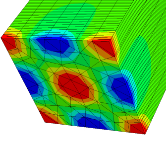
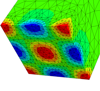
Figure 2: Comparison of a mesh made from time slabs (left) and an adapted space-time mesh (middle). The convergence of the two methods with respect to the number of degrees of freedom is shown on the right for $p=1$.

In Figure 2 we highlight another feature of the space-time approach, namely the ability to use adapted mesh in space and time. As a comparison, we use a mesh made of time slabs, a mesh structure similar to what would result from classic time-stepping methods. The timeslab height is given by $h_{t}\approx h_{x}^{2}$, with $h_{x}$ being the mesh size of the spatial mesh. For the space-time adapted mesh, we start with a unstructured simplicial mesh of size $h=0.2$ and then apply adaptive refinement. For this simple example, we use a flux based error estimator and Dörfler marking with $\theta=0.5$. We observe the same rate of convergence on both meshes, however using the space-time adapted mesh allows us to obtain a given accuracy with fewer degrees of freedom.

4.2 The porous medium equation

Let $m>1$. The porous medium equation is given by

$$\begin{cases}\partial_{t}\rho=\Delta\rho^{m}&\mbox{in }\Omega\ t>0,\\ \partial_{\nu}(\rho^{m})=0&\mbox{on }\partial\Omega,\ t>0,\\ \rho(0)=\rho_{0}&\mbox{in }\Omega.\end{cases}$$

We can write it in the form of (1) for $N=1$, $A(\rho)=m\rho^{m-1}$, and $f\equiv 0$. The entropy density is the same as for the heat equation.

Proposition 4.2.

Assumptions (H1) and (H2) are satisfied for $m\in(1,2]$.

Proof 4.3.

For $\mathcal{D}=(0,1)$ and $m>1$, $A(\rho)=m\rho^{m-1}$ is in $C^{0}(\overline{\mathcal{D}})$, thus (H1) is stisfied. As (H2b) is obvious, we only need to prove that (H2a) is satisfied, namely that $s^{\prime\prime}(\rho)A(\rho)\geq\gamma$ for some $\gamma>0$ and all $\rho\in\mathcal{D}$. Thus let $\rho\in(0,1)=\mathcal{D}$. Then, whenever $m\in(1,2]$,

$$s^{\prime\prime}(\rho)A(\rho) =\frac{m\rho^{m-1}}{\rho(1-\rho)}=\frac{m}{\rho^{2-m}(1-\rho)}\geq m=:\gamma.$$

We test the space-time Galerkin method for this problem with initial conditions and Neumann boundary conditions chosen such that

$$\rho(x,t)=\left[\frac{(m-1)(x-\alpha)^{2}}{2m(m+1)(\beta-t)}\right]^{\frac{1}{m-1}}$$

is the exact solution, with $\alpha$ and $\beta$ real parameters, on $\Omega=(0,1)$. We consider the case $m=2,\ \alpha=2,\ \beta=5$ on unstructured simplicial space-time meshes.

In Figure 3, we show the convergence rates of the scheme. Regardless of the nonlinearity, we match the convergence rates of the heat equation, i.e. exponential in $p$ and of order $p+1$ in $h$. The convergence rates in terms of $h$ are also considered for different values of $\varepsilon$. We observe that $\varepsilon$ introduces a lower bound on the error. Therefore, choosing it as small as possible, such that the solver still converges, gives the best results. On the other hand, in the next example, we can see that for certain solutions, that produce a very ill-conditioned system, we must choose $\varepsilon$ fairly large.

Figure 3: Convergence rates towards the exact solution of the porous medium equation. Convergence in terms of the polynomial degree $p$ for different mesh sizes is shown on the left. We consider convergence in mesh size $h$ for different values of the polynomial order $p$ and fixed $\varepsilon=0$ in the middle, and for fixed $p=4$ and different values of regularization parameter $\varepsilon$ on the right.

In contrast to the heat equation, the power law in the porous medium equation introduces a finite propagation speed of the solution. This is best observed by the interesting behavior of certain initial conditions that induce a waiting time. That is, the solution keeps a fixed support until the waiting time is reached. On $\Omega=(0,\pi)$, the initial condition given by

$$\rho_{0}(x)=\begin{cases}\sin^{2/(m-1)}(x)&\text{ if }0\leq x\leq\pi,\\ 0&\text{ otherwise, }\end{cases}$$

produces this behavior. It is shown in [39] that the corresponding solution has a waiting time of $t^{*}=\frac{m-1}{2m(m+1)}$. As we choose $m=2$, here $t^{*}=0.08\dot{3}$. We modify the initial condition to $\rho_{0}(x)=10^{-16}$ for $x\notin[0,\pi]$ to avoid ill-conditioning. Furthermore, to ensure convergence of the Newton method used as a nonlinear solver, we had to choose $\varepsilon={10^{-6}}$, making use of the regularization term. We solve on a Cartesian space-time mesh until final time $T=0.2$, with spatial mesh size $h_{s}=0.05$, and temporal mesh size $h_{t}=h_{s}/2$, and fix $p=5$. The results are shown in Figure 4. Looking at snapshots of the numerical solution we can observe that it keeps a compact support set. In Figure 4, on the right, we plot the value of the solution on the left interface against time, marking the expected waiting time $t^{*}$ with the vertical line.

Figure 4: Snapshots of the solution of the porous medium equation emitting a waiting time, at different times (left) and the value at the left interface (right).

4.3 The Fisher-KPP equation

We consider the Fisher-KPP equation

$$\begin{cases}\partial_{t}\rho=A\Delta\rho+\rho(1-\rho)&\mbox{in }\Omega,\ t>0,\\ A\partial_{\nu}\rho=0&\mbox{on }\partial\Omega,\ t>0,\\ \rho(0)=\rho_{0}&\mbox{in }\Omega,\end{cases}$$

with $A>0$ now constant. This agrees with formulation (1), with $N=1$, $A(\rho)=A$, and $f(\rho)=\rho(1-\rho)$. We set again $\mathcal{D}:=(0,1)$. Assumptions (H1) and (H2a) are clearly satisfied. Choosing an entropy density such that assumption (H2b) is satisfied with $C_{f}=0$ allows for the right-hand side of the entropy estimate (8) to be independent of time. Motivated by this, we now investigate the rescaled entropy density $s:\mathcal{D}\to(0,+\infty)$ given by

(18) $$s(\rho)={\rho}\log{\rho}+(n-{\rho})\log(n-{\rho}),$$

with $n$ to be chosen. Note that $f(\rho)>0$ for $\rho\in(0,1)$, and $n/\rho-1>1$ if and only if $\rho<n/2$. Thus,

$$f(\rho)s^{\prime}(\rho) =\rho(1-\rho)\log\frac{\rho}{n-\rho}=-\rho(1-\rho)\log{(\frac{n}{\rho}-1)}\leq 0$$

for all for $\rho\in(0,1)$ if and only if $n\geq 2$. We choose $n=2$ so that the hypothesis (H2b) is fulfilled with $C_{f}=0$.

We start again by investigate convergence towards a smooth solution. We choose $\Omega=(0,1)$, and initial conditions and Neumann boundary conditions such that

$$\rho(x,t)=\frac{1}{\left[1+\exp(-\frac{5}{6}t+\frac{1}{\sqrt{6}}x)\right]^{2}}$$

is the exact solution for $A=1$. We set $\varepsilon=0$ and solve on unstructured simplicial space-time meshes. The results are presented in Figure 5. We observe again optimal convergence rates in both $p$ and $h$, namely exponential in $p$ and of order $p+1$ in $h$.

Figure 5: Convergence rates in polynomial degree $p$ (left) and mesh size $h$ for the exact solution of the Fisher-KPP equation.

Next, we aim to reproduce the experiments presented in [5], considering an initial condition with a jump, given by $\rho_{0}(x)=1\text{ if }0<x<1/2$ and 0 elsewhere, with diffusion coefficient $A=10^{-4}$. We solve using $p=3$ on a Cartesian mesh with $h_{s}=0.025$, $h_{t}=0.4$ up to $T=8$. We choose $\varepsilon=10^{-8}$ to avoid ill-conditioning in the solver.

Figure 6: Snapshots of the numerical solution for the Fisher-KPP (left) and different choices of the entropy (right). The choices are as follows: Entropy 1 is the one used in [5], Entropy 2 is given by (18) with $n=2$, and Entropy 3 is (18) with $n=2.1$.

Snapshots of the numerical solution are taken every $1.\dot{3}$ seconds, the results are shown in Figure 6 on the left. In Figure 6 on the right, we consider different choices for the entropy up to $T=15$. Note that at the point in time the solution has already converged to $\rho\equiv 1$. The choice for the entropy density in [5] was $\rho\log(\rho)-\rho+1$. This choice is not covered by our assumptions, however, using it produces the correct results, as conjectured in Remark 2.1. We compare it to the entropy in (18) for different values of $n$ in Figure 6. For the choice of $n=2$, we recover a similar behavior of the entropy, namely, a region with slow decay followed by an exponential decay. As the solution converges to $1$ it can easily be seen that for $n>2$ the entropy does not converge to zero exponentially, as exemplified by the choice of $n=2.1$ in the figure, since it is not the correct relative entropy with respect to the equilibrium.

4.4 The three-component Maxwell-Stefan system

The Maxwell-Stefan system for $N=2$ can be written as

$$\begin{cases}\partial_{t}\rho_{i}=\nabla\cdot\left(\sum_{j=1}^{2}A_{ij}(\rho_{1},\rho_{2})\nabla\rho_{j}\right)&\mbox{in }\Omega,\ t>0,\\ \sum_{j=1}^{2}A_{ij}(\rho_{1},\rho_{2})\partial_{\nu}\rho_{j}=0&\mbox{on }\partial\Omega,\ t>0,\\ \rho_{i}(0)=(\rho_{0})_{i}&\mbox{in }\Omega\end{cases}$$

for $i=1,2$, with

(19) $$A(\rho_{1},\rho_{2})=\frac{1}{\delta(\rho_{1},\rho_{2})}\begin{pmatrix}d_{1}+(d_{3}-d_{1})\rho_{1}&(d_{3}-d_{2})\rho_{1}\\ (d_{3}-d_{1})\rho_{2}&d_{2}+(d_{3}-d_{2})\rho_{2}\end{pmatrix}$$

and

$$\delta(\rho_{1},\rho_{2})=d_{1}d_{2}(1-\rho_{1}-\rho_{2})+d_{2}d_{3}\rho_{1}+d_{3}d_{1}\rho_{2}.$$

The unknowns $\rho_{1}$ and $\rho_{2}$ represent the concentrations of the first two gases ($\rho_{3}=1-(\rho_{1}+\rho_{2})$); the parameters $d_{1}$, $d_{2}$, and $d_{3}$ are the related to the binary diffusion coefficients of the three gases. In section 5 below, we derive this form of the Maxwell-Stefan system, prove that it fits our framework, and discuss the case $N>2$.

Figure 7: The mesh used for the Duncan-Toor example, depicting the carbon dioxide content after about ten hours.

Figure 8: Comparison of the mole fractions in the left side of the device.

In [7, Sec. 2] numerical results were presented for the three component gas diffusion experiment originally performed by Duncan and Toor in [15]. The setting is the following. Consider two spherical bulbs of volume 77.99 cm³ (radius 26.49 mm) and 78.63 cm³ (radius 26.58 mm), respectively, which are connected by a capillary tube of length 85.9 mm and diameter 2.08 mm, with a valve in the middle. We consider the Maxwell-Stefan equations with $N=2$, corresponding to the gas mixture composed of hydrogen ($\rho_{1}$), nitrogen ($\rho_{2}$), and carbon dioxide ($\rho_{3}$). We consider the following initial gas mixture in the left- and right-hand side of the device:

$$\text{Left:}\quad(\rho_{0})_{1}=0.000,\quad(\rho_{0})_{2}=0.501,\quad(\rho_{0})_{3}=0.499,$$

$$\text{Right:}\quad(\rho_{0})_{1}=0.501,\quad(\rho_{0})_{2}=0.499,\quad(\rho_{0})_{3}=0.000.$$

For these gases, the coefficients $d_{1}$, $d_{2}$, and $d_{3}$ are given in terms of the binary diffusion coefficients (see section 5.1 below) as follows: d_1^-1=D_13=68.0 mm^2s^-1,  d_2^-1=D_23=16.8 mm^2s^-1,  d_3^-1=D_12=83.3 mm^2s^-1.

As in [7], we can reduce the domain to two dimensions, as the device and initial conditions are axially symmetric and the flux vector has no angular component. In Figure 7, the computational domain is shown. We choose the spatial mesh size $h_{s}=2.08$ mm, equal to the diameter of the tube. The size of the Cartesian product mesh in time is chosen as 20.8 s. We solve iteratively on these slabs, restarting the computations with the previous solution as initial condition. We fix $p=2$ and $\varepsilon=10^{-10}$.

The results are shown in Figure 8. We recover the same behavior shown in [7]. Both hydrogen and carbon dioxide converge monotonically to the expected equilibrium. Nitrogen shows the peculiar behavior known from the experiment.

Figure 9: Entropy and entropy dissipation (in absolutes) for the Duncan-Toor example, both showing exponential convergence to the equilibrium.

In Figure 9, we show the relative entropy and its dissipation, i.e. the time derivative of the entropy, both converge exponentially. This can be expected, as this behavior has been proven for similar types of equations, see for example [3, eq. (1.16)] where it is formally stated that the entropy dissipation converges exponentially for the Fokker-Planck equation by the use of the Bakry-Emery method.

5 The Maxwell-Stefan system revisited

In this section, we derive the formulation of the Maxwell-Stefan system as that used in section 4.4, and show that it fits into the general framework of section 2 (section 5.1). For the case $N>2$, in which an explicit representation of the currents may not be easily derived, we introduce and analyze an alternative space-time Galerkin method, which is based on a formulation that is implicit for the currents (section 5.2).

Let $\rho_{0}\in L^{\infty}(\Omega)^{N+1}$ such that $\rho_{0}\geq 0$ and $\sum_{i=1}^{N+1}(\rho_{0})_{i}=1$. The Maxwell-Stefan equations are given by the continuity equations

(20) $$\left\{\begin{aligned} \partial_{t}\rho_{i}+\nabla\cdot J_{i}=0&\qquad\mbox{in }(0,T)\times\Omega,\\ \nu\cdot J_{i}=0&\qquad\mbox{on }(0,T)\times\partial\Omega,\\ \rho_{i}(0)=(\rho_{0})_{i}&\qquad\mbox{in }\Omega\end{aligned}\right.$$

for $i=1,\ldots,N+1$, where the currents $J_{i}$ are implicitly given by

(21) $$\nabla\rho_{i}=\sum_{j=1}^{N+1}\frac{\rho_{i}J_{j}-\rho_{j}J_{i}}{D_{ij}}$$

for some $D_{ij}=D_{ji}>0$.

5.1 Explicit formula for the currents

In this section, we establish an explicit representation of the currents, which allows us to derive the formulation of the Maxwell-Stefan system in the concentration variable unknowns. We follow [6] (see also [30]).

Let $M_{ij}(\rho):=D_{ij}^{-1}\rho_{i}-\delta_{ij}\sum_{k=1}^{N+1}D_{ik}^{-1}\rho_{k}$, $i,j=1,\ldots,N+1$. Thus,

$$\nabla\rho_{i}=\sum_{j=1}^{N+1}M_{ij}(\rho)J_{j}.$$

Using $\rho_{i}\geq 0$ and $D_{ij}=D_{ji}>0$, it is easy to see that $M(\rho)$ is quasi-positive ($M_{ij}(\rho)\geq 0$ for $i\neq j$). Moreover, provided that $\rho_{i}>0$ for all $1\leq i\leq N+1$, $M(\rho)$ is irreducible. Direct calculations show that

$$\mathrm{Ker}\,M(\rho)\supseteq\mathrm{span}\{\rho\}\qquad\mbox{and}\qquad\mathrm{Im}\,M(\rho)\subseteq\left\{v:\sum_{i=1}^{N+1}v_{i}=0\right\}.$$

Moreover, $R^{-1}M(\rho)R$, with $R=\text{diag}(\rho_{1}^{1/2},\ldots,\rho_{N+1}^{1/2})$, is symmetric, thus all the eigenvalues of $M(\rho)$ are real. By the Perron-Frobenius theory for quasi-positive, irreducible matrices, one deduces that the eigenvalue zero has multiplicity one (we refer to [6] or [30] for details). We deduce

(22) $$\mathrm{Ker}\,M(\rho)=\mathrm{span}\{\rho\}\qquad\mbox{and}\qquad\mathrm{Im}\,M(\rho)=\left\{v:\sum_{i=1}^{N+1}v_{i}=0\right\}.$$

As $M(\rho)$ is not invertible, we have to restrict ourselves to a subspace of all possible currents $J$ in order to obtain an explicit formula for $J$. For this, we make the assumption that the total current

$$J_{\mathrm{tot}}:=\sum_{i=1}^{N+1}J_{i}$$

vanishes. Then by summing in (20) over all $i=1,\ldots,N+1$, we see that

$$\rho_{\mathrm{tot}}=\sum_{i=1}^{N+1}\rho_{i}$$

is constant in time, and hence $\rho_{\mathrm{tot}}=\sum_{i=1}^{N+1}(\rho_{0})_{i}=1$. Using this, we can rewrite the implicit formulation of the currents as

(23) $$\nabla\rho_{i}=\frac{\rho_{i}\left(-\sum_{j=1}^{N}J_{j}\right)-\left(1-\sum_{j=1}^{N}\rho_{j}\right)J_{i}}{D_{i(N+1)}}+\sum_{j=1}^{N}\frac{\rho_{i}J_{j}-\rho_{j}J_{i}}{D_{ij}}$$

As before, we can define a matrix

(24) $$\mathcal{M}_{ij}(\rho):=\frac{\rho_{i}}{D_{ij}}-\frac{\rho_{i}}{D_{i(N+1)}}-\delta_{ij}\left(\sum_{k=1}^{N}\frac{\rho_{k}}{D_{ik}}+\frac{1-\sum_{l=1}^{N}{\rho_{l}}}{D_{i(N+1)}}\right),\qquad i,j=1,\ldots,N.$$

From (22), the matrix $\mathcal{M}(\rho)$ has full rank, and hence it is invertible. We have

$$J_{i}=-\sum_{j=1}^{N}A_{ij}(\rho)\nabla\rho_{j}\qquad\mbox{with }A(\rho):=-\mathcal{M}(\rho)^{-1}.$$

Remark 5.1.

The matrix $\mathcal{M}(\rho)$ is actually independent from the diagonal elements $D_{ii}$.

Proposition 5.2.

Let $s$ be as in (15), and let $\mathcal{M}$ be given by (24). Then, the matrix-valued function $A(\rho):=-\mathcal{M}(\rho)^{-1}$ fulfills (H1) and (H2a).

Proof 5.3.

Let $A(\rho)=-\mathcal{M}^{-1}(\rho)$. The fact that $\mathcal{M}$ is smooth directly implies that $A$ is smooth. Similarly as in the proof of [30, Lemma 3.2], one can show that

(25) $$\sum_{i=1}^{d}\partial_{i}w\cdot A(u(w))s^{\prime\prime}(u(w))^{-1}\partial_{i}w\geq\gamma|\nabla{u(w)}|^{2}$$

for some $\gamma>0$ and all smooth $w$.

In order to prove (H2a), we have to show that

$$z\cdot s^{\prime\prime}(\rho)A(\rho)z\geq\gamma|z|^{2}\qquad\mbox{for all }z\in\mathbb{R}^{N},\,\rho\in\mathcal{D}.$$

Let $\rho\in\mathcal{D}$, ${\bm{x}}_{0}\in\Omega$, and $z\in\mathbb{R}^{N}$. We define the following vector-valued function of ${\bm{x}}$:

$$w({\bm{x}}):=s^{\prime}(\rho)+s^{\prime\prime}(\rho)z(\bm{x}-\bm{x}_{0})\cdot\hat{e}_{1},$$

where $\hat{e}_{1}$ denotes the unit vector $(1,0,\ldots,0)\in\mathbb{R}^{d}$. We have

$$\partial_{i}w({\bm{x}}_{0})=\delta_{i1}s^{\prime\prime}(\rho)z$$

and, for $u=(s^{\prime})^{-1}$,

$$\partial_{i}u(w({\bm{x}}_{0}))=u^{\prime}(w(\bm{x}_{0}))\partial_{i}w(\bm{x}_{0})=u^{\prime}(w(\bm{x}_{0}))\delta_{i1}s^{\prime\prime}(\rho)z=u^{\prime}(w(\bm{x}_{0}))\delta_{i1}s^{\prime\prime}(u(w(\bm{x}_{0})))z=\delta_{i1}z.$$

This, together with (25), implies that

$$z\cdot s^{\prime\prime}(\rho)A(\rho)z =(s^{\prime\prime}(\rho)z)\cdot A(\rho)s^{\prime\prime}(\rho)^{-1}(s^{\prime\prime}(\rho)z)$$

$$=\sum_{i=1}^{d}\partial_{i}w({\bm{x}}_{0})\cdot A(u(w({\bm{x}}_{0})))s^{\prime\prime}(u(w({\bm{x}}_{0})))^{-1}\partial_{i}w({\bm{x}}_{0})$$

$$\geq\gamma|\nabla{u(w({\bm{x}}_{0}))}|^{2}=\gamma|z|^{2},$$

which proves the assertion.

For $N=1$, the matrix $\mathcal{M}(\rho)$ is actually a scalar, which is given by

$$\mathcal{M}(\rho)=-\frac{\rho_{1}}{D_{12}}-\frac{1-\rho_{1}}{D_{12}}=-\frac{1}{D_{12}}.$$

Hence, $J_{1}=D_{12}\nabla\rho_{1}$. Therefore, in this case the Maxwell-Stefan system reduces to the heat equation.

For three species/gases ($N=2$), we have

$$\mathcal{M}(\rho_{1},\rho_{2}) =\begin{pmatrix}\frac{\rho_{1}}{D_{11}}-\frac{\rho_{1}}{D_{13}}-\frac{\rho_{1}}{D_{11}}-\frac{\rho_{2}}{D_{12}}-\frac{1-\rho_{1}-\rho_{2}}{D_{13}}&\frac{\rho_{1}}{D_{12}}-\frac{\rho_{1}}{D_{13}}\\ \frac{\rho_{2}}{D_{21}}-\frac{\rho_{2}}{D_{23}}&\frac{\rho_{2}}{D_{22}}-\frac{\rho_{2}}{D_{23}}-\frac{\rho_{1}}{D_{21}}-\frac{\rho_{2}}{D_{22}}+\frac{1-\rho_{1}-\rho_{2}}{D_{23}}\end{pmatrix}$$

$$=-\begin{pmatrix}\frac{1}{D_{13}}+\big{(}\frac{1}{D_{12}}-\frac{1}{D_{13}}\big{)}\rho_{2}&\big{(}\frac{1}{D_{13}}-\frac{1}{D_{12}}\big{)}\rho_{1}\\ \big{(}\frac{1}{D_{23}}-\frac{1}{D_{21}}\big{)}\rho_{2}&\frac{1}{D_{23}}+\big{(}\frac{1}{D_{21}}-\frac{1}{D_{23}}\big{)}\rho_{1}\end{pmatrix}.$$

Let

$$d_{1}:=\frac{1}{D_{13}},\qquad d_{2}:=\frac{1}{D_{23}},\qquad d_{3}:=\frac{1}{D_{12}},$$

and recall that $D_{21}=D_{12}$. One can verify that

$$\delta(\rho_{1},\rho_{2}):=\det\mathcal{M}(\rho_{1},\rho_{2})=d_{1}d_{2}(1-\rho_{1}-\rho_{2})+d_{2}d_{3}\rho_{1}+d_{3}d_{1}\rho_{2}\neq 0.$$

Let $A(\rho)$ denote the inverse of $-\mathcal{M}(\rho)$. We can rewrite the Maxwell-Stefan equations as the system in section 4.4.

5.2 Implicit formulation for the currents

In subsection 5.1, we have seen that the Maxwell-Stefan system (20)-(21), can be written in the form (1), with $f=0$ and $A(\rho)$ being given by the inverse of $-\mathcal{M}(\rho)$ for

$$\mathcal{M}_{ij}(\rho):=\frac{\rho_{i}}{D_{ij}}-\frac{\rho_{i}}{D_{i(N+1)}}-\delta_{ij}\left(\sum_{k=1}^{N}\frac{\rho_{k}}{D_{ik}}+\frac{1-\sum_{l=1}^{N}{\rho_{l}}}{D_{i(N+1)}}\right),\qquad i,j=1,\ldots,N.$$

Moreover, we have computed $A(\rho)$ explicitly for $N=1$ and $N=2$. However, for large $N$, it is more complicated to find the explicit formulation for $A(\rho)$. In any case we do not expect a simple formulation in these cases. Therefore, this section provides a space-time Galerkin scheme, which avoids the explicit computation of the inverse of $\mathcal{M}$.

Let $q,p\in\mathbb{N}$. We consider the following problem:

(26) $$\text{Find}\quad w_{h}^{\varepsilon}\in\bm{V}_{h}^{p},J^{\mu}\in\bm{V}_{h}^{q},\ \mu=1,\ldots,d,\quad\text{such that}\\ \begin{aligned} 0&=\varepsilon(\phi^{0},w_{h}^{\varepsilon})_{{H^{1}_{\varepsilon}}(Q_{T})}+\int_{\Omega}\phi^{0}(T)\cdot u(w_{h}^{\varepsilon}(T))dx-\int_{\Omega}\phi^{0}(0)\cdot\rho_{0}dx-\int_{Q_{T}}\partial_{t}\phi^{0}\cdot u(w_{h}^{\varepsilon})dxdt\\ &\qquad-\sum_{\mu=1}^{d}\left(\int_{Q_{T}}\partial_{x_{\mu}}\phi^{0}\cdot J^{\mu}dxdt+\int_{Q_{T}}\phi^{\mu}\cdot\big{(}\partial_{x_{\mu}}w_{h}^{\varepsilon}-s^{\prime\prime}(u(w_{h}))\mathcal{M}(u(w_{h}^{\varepsilon}))J^{\mu}\big{)}dxdt\right)\end{aligned}\\ \forall\phi^{0}\in\bm{V}_{h}^{p},\ \phi^{\mu}\in\bm{V}_{h}^{q},\ \mu=1,\ldots,d.$$

Proposition 5.4.

Assume that $\rho_{0}:\Omega\to\overline{\mathcal{D}}$ is measurable. Then there exists a solution $w_{h}^{\varepsilon}\in\bm{V}_{h}^{p},J^{\mu}\in\bm{V}_{h}^{q}$, $\mu=1,\ldots,d$ of the method (26).

For the proof of Proposition 5.4, we need the following lemma.

Lemma 5.5.

If $w_{h}^{\varepsilon}\in\bm{V}_{h}^{p},J^{\mu}\in\bm{V}_{h}^{q},\ \mu=1,\ldots,d$, solves (26), then

$$\varepsilon\|w_{h}^{\varepsilon}\|_{{H^{1}_{\varepsilon}}(Q_{T})}^{2}+\int_{\Omega}s(u(w_{h}^{\varepsilon}(T)))dx+\gamma\sum_{\mu=1}^{d}\int_{Q_{T}}|\mathcal{M}(u(w_{h}^{\varepsilon}))J^{\mu}|^{2}dxdt\leq\int_{\Omega}s(\rho_{0})dx.$$

Proof 5.6.

We can use $\phi^{0}=w_{h}^{\varepsilon}$ and $\phi^{\mu}=0$ for $\mu=1,\ldots,d$ as test functions and, similarly to the proof of Proposition 3.3, we obtain that

$$\varepsilon\|w_{h}^{\varepsilon}\|_{{H^{1}_{\varepsilon}}(Q_{T})}^{2}+\int_{\Omega}s(u(w_{h}^{\varepsilon}(T)))dx-\sum_{\mu=1}^{d}\int_{Q_{T}}J^{\mu}\cdot\partial_{x_{\mu}}w_{h}^{\varepsilon}dxdt\leq\int_{\Omega}s(\rho_{0})dx.$$

The next step is to use the test functions $\phi^{0}=0$ and $\phi^{\mu}=J^{\mu}$ for $\mu=1,\ldots,d$ to obtain

$$\sum_{\mu=1}^{d}\int_{Q_{T}}J^{\mu}\cdot\partial_{x_{\mu}}w_{h}^{\varepsilon}dxdt=\sum_{\mu=1}^{d}\int_{Q_{T}}J^{\mu}\cdot s^{\prime\prime}(u(w_{h}^{\varepsilon}))\mathcal{M}(u(w_{h}^{\varepsilon}))J^{\mu}dxdt.$$

According to assumption (H2a), we know that $s^{\prime\prime}(v)A(v)$ is positive semi-definite and satisfies

$$z\cdot s^{\prime\prime}(v)A(v)z\geq\gamma|z|^{2}\quad\mbox{for all }z\in\mathbb{R}^{N},\,v\in\mathcal{D}.$$

Choosing $v=u(w_{h}^{\varepsilon})$, $z:=\mathcal{M}(u(w_{h}^{\varepsilon}))J^{\mu}$, we see that

$$\gamma|\mathcal{M}(u(w_{h}^{\varepsilon}))J^{\mu}|^{2} \leq J^{\mu}\cdot\mathcal{M}(v)s^{\prime\prime}(v)A(v)\mathcal{M}(v)J^{\mu}=-J^{\mu}\cdot\mathcal{M}(v)s^{\prime\prime}(v)J^{\mu},$$

where in the last step we have used that $A(v)$ is the inverse of $-\mathcal{M}(v)$. Thus, we conclude that

$$\varepsilon\|w_{h}^{\varepsilon}\|_{{H^{1}_{\varepsilon}}(Q_{T})}^{2}+\int_{\Omega}s(u(w_{h}^{\varepsilon}(T)))dx+\gamma\sum_{\mu=1}^{d}\int_{Q_{T}}|\mathcal{M}(u(w_{h}^{\varepsilon}))J^{\mu}|^{2}dxdt \leq\int_{\Omega}s(\rho_{0})dx.$$

Proof 5.7 (Proof of Proposition 5.4).

The idea of the proof is to proceed similarly to the proof of Proposition 3.3. We define the mapping

$$\Phi:\bm{V}_{h}^{p}\times(\bm{V}_{h}^{q})^{d}\to\bm{V}_{h}^{p}\times(\bm{V}_{h}^{q})^{d},\ (v,I^{1},\ldots,I^{d})\mapsto(w,J^{1},\ldots,J^{d}),$$

where $w$ is (uniquely) defined via the equation

$$0=\varepsilon(\phi^{0},w)_{{H^{1}_{\varepsilon}}(Q_{T})}+\int_{\Omega}\phi^{0}(T)\cdot u(v(T))dx-\int_{\Omega}\phi^{0}(0)\cdot\rho^{0}dx-\int_{Q_{T}}\partial_{t}\phi^{0}\cdot u(v)dxdt\\ -\sum_{\mu=1}^{d}\int_{Q_{T}}\partial_{x_{\mu}}\phi^{0}\cdot I^{\mu}dxdt\quad\mbox{for all }\phi^{0}\in\bm{V}_{h}^{p},$$

and $J^{\mu}$ denotes the unique solution (see below for a justification) of

(27) $$\int_{Q_{T}}\phi^{\mu}\cdot\partial_{x_{\mu}}vdxdt=\int_{Q_{T}}\phi^{\mu}\cdot s^{\prime\prime}(u(v))\mathcal{M}(u(v))J^{\mu}dxdt\qquad\mbox{for all }\phi^{\mu}\in\bm{V}_{h}^{q}.$$

Note that the mapping $\Phi$ is well-defined, as (27) admits a unique solution for given $v\in\bm{V}_{h}^{p}$ according to the Lemma of Lax-Milgram: we see that $\partial_{x_{\mu}}v\in L^{2}(Q_{T})^{N}$ and the matrix ${-s^{\prime\prime}(u(v))\mathcal{M}(u(v))\in L^{\infty}(Q_{T})^{N\times N}}$ is positive definite, because for all $z\in\mathbb{R}^{N}$

$$z\cdot\big{(}-s^{\prime\prime}(u(v))\mathcal{M}(u(v))\big{)}z =A(u(v))y\cdot s^{\prime\prime}(u(v))y$$

$$=y\cdot s^{\prime\prime}(u(v))A(u(v))y$$

$$\!\!\stackrel{{\scriptstyle\text{(H2a)}}}{{\geq}}\gamma|y|^{2}=\frac{\gamma}{\|A(u(v))\|^{2}}\|A(u(v))\|^{2}|y|^{2}$$

$$\geq\frac{\gamma}{\|A(u(v))\|^{2}}|A(u(v))y|^{2}=\frac{\gamma}{\|A(u(v))\|^{2}}|z|^{2}$$

for $y:=A(u(v))^{-1}z=-\mathcal{M}(u(v))z$. Moreover, the mapping $\Phi$ is continuous since $A$ and $u$ are continuous. Then by the Leray-Schauder fixed-point theorem, we obtain that $\Phi$ admits a fixed-point if we can show that the set

$$\{(w,J^{1},\ldots J^{d})\in\bm{V}_{h}\times(\bm{V}_{h}^{q})^{d}:(w,J^{1},\ldots J^{d})=\sigma\Phi(w,J^{1},\ldots J^{d}),\sigma\in[0,1]\}$$

is bounded. Let $(w,J^{1},\ldots,J^{d})=\sigma\Phi(w,J^{1},\ldots,J^{d})$ for $\sigma\in(0,1]$. Similarly to Lemma 5.5, we can prove the entropy estimate

$$\frac{\varepsilon}{\sigma}\|w\|_{{H^{1}_{\varepsilon}}(Q_{T})}^{2}+\int_{\Omega}s(u(w(T)))dx+\frac{\gamma}{\sigma}\sum_{\mu=1}^{d}\int_{Q_{T}}|\mathcal{M}(u(w))J^{\mu}|^{2}dxdt\leq\int_{\Omega}s(\rho_{0})dx.$$

Using that $\sigma\in(0,1]$ is bounded from above yields a uniform bound on $w$ in $\bm{V}_{h}^{q}$ and on $\mathcal{M}(u(w))J^{\mu}$ in $L^{2}(Q_{T})^{N}$. As $\bm{V}_{h}^{q}$ is finite dimensional, we directly obtain that $\|w\|_{L^{\infty}(Q_{T})^{N}}$ is uniformly bounded. Thus,

$$\|J^{\mu}\|_{L^{2}(Q_{T})^{N}}\leq\|A(u(w))\|_{L^{\infty}(Q_{T})^{N\times N}}\|\mathcal{M}(u(w))J^{\mu}\|_{L^{2}(Q_{T})^{N}}$$

is also uniformly bounded. As all norms are equivalent on $\bm{V}_{h}^{q}$, this directly implies that $J^{\mu}$ is uniformly bounded in $\bm{V}_{h}^{q}$. Thus, the Leray-Schauder theorem is applicable and yields that $\Phi$ has a fixed-point, and therefore the scheme (26) admits a solution.

Proposition 5.8.

Let $\rho_{0}:\Omega\to\overline{\mathcal{D}}$ be measurable and $w_{h}^{\varepsilon}\in\bm{V}_{h}^{p},J^{\varepsilon,\mu}_{h}\in\bm{V}_{h}^{q},\ \mu=1,\ldots,d$, be a solution of (26) for $\varepsilon,h>0$. Then there exist a solution $\rho$ of (5) and sequences $h_{i},\varepsilon_{i}\to 0$, as $i\to\infty$, such that

$$u(w^{\varepsilon_{i}}_{h_{i}})\to\rho\qquad\mbox{in }L^{r}(Q_{T})\mbox{, as }i\to\infty$$

for all $r\in[1,\infty)$. Moreover, $\rho$ satisfies the entropy estimate

(28) $$\int_{\Omega}s(\rho(\tau))dx+\gamma\int_{0}^{\tau}\int_{\Omega}\left|\nabla\rho\right|^{2}dxdt\leq\int_{\Omega}s(\rho_{0})dx$$

for all $\tau\in(0,T]$, where $|\Omega|$ is the volume of $\Omega$.

Proof 5.9.

The proof is analogue to the proof of Proposition 3.4. We only need to replace Proposition 3.7 by Lemma 5.10 below.

Lemma 5.10 (Convergence of the scheme for fixed $\varepsilon>0$).

Let $w_{h}\in\bm{V}_{h}^{p},J^{\mu}_{h}\in\bm{V}_{h}^{q},\ \mu=1,\ldots,d$ be a solution of (26), with fixed $\varepsilon>0$. Then there exists $\rho\in H^{1}(Q_{T})^{N}$ with $\rho(t,x)\in\overline{\mathcal{D}}$ for a.e. $(t,x)\in Q_{T}$ and $s^{\prime}(\rho)\in H^{1}(Q_{T})^{N}$, and a sequence $h_{\ell}\to 0$ such that ρ_h_ℓ:= u(w_h_ℓ)→ρ  and  w_h_ℓ→s’(ρ) strongly in $L^{2}(Q_{T})$ and weakly in ${H^{1}_{\varepsilon}}(Q_{T})$. Moreover, $\rho$ solves (6) and satisfies the entropy estimate (10) for $w=s^{\prime}(\rho)$.

Proof 5.11.

The fact that $w_{h}$ is uniformly bounded in ${H^{1}_{\varepsilon}}(Q_{T})^{N}$ yields that there exists $w\in H^{1}(Q_{T})^{N}$ and subsequence ${h_{\ell}}\to 0$ such that $w_{h_{\ell}}\rightharpoonup w$ in ${H^{1}_{\varepsilon}}(Q_{T})^{N}$, due to the Banach-Alaoglu theorem, and $w_{h_{\ell}}\to w$ in $L^{2}(Q_{T})^{N}$ due to Rellich’s theorem. As $u$ is bounded, the dominated convergence theorem entails the convergence for $\rho_{h_{\ell}}\equiv u(w_{h_{\ell}})$ to $\rho:=u(w)$ along another subsequence (which we do not relabel).

For the second part, we note that, due to the Banach-Alaoglu theorem and the boundedness of $\mathcal{M}(u(w_{h}))J^{\mu}_{h}$ in $L^{2}(Q_{T})^{N}$, we know that there exist $\xi^{\mu}\in L^{2}(Q_{T})^{N}$ such that, for a subsequence (not being relabeled),

$$\mathcal{M}(u(w_{h}))J^{\mu}_{h}\rightharpoonup\xi^{\mu}\qquad\mbox{weakly in }L^{2}(Q_{T})^{N}.$$

In particular,

$$J^{\mu}_{h}=-A(u(w_{h}))\mathcal{M}(u(w_{h})){J^{\mu}_{h}}\rightharpoonup-A(\rho)\xi^{\mu}=:J^{\mu}\qquad\mbox{weakly in }L^{r}(Q_{T})^{N}$$

for every $r\in[1,2)$. Finally, for every $\phi^{\mu}\in H^{1}(Q_{T})^{N}$, $j=0,\ldots,d$, there exist $\phi^{\mu}_{h_{\ell}}\in\bm{V}^{p}_{h_{\ell}}\cap\bm{V}^{q}_{h_{\ell}}$ such that $\phi^{\mu}_{h_{\ell}}\to\phi^{\mu}$ in ${H^{1}_{\varepsilon}}(Q_{T})^{N}$. Using $\phi^{\mu}_{h_{\ell}}$ as a test function in (26), in the limit $h_{\ell}\to 0$, we obtain

$$0 =\varepsilon(\phi^{0},w)_{{H^{1}_{\varepsilon}}(Q_{T})}+\int_{\Omega}\phi^{0}(T)\cdot u(w(T))dx-\int_{\Omega}\phi^{0}(0)\cdot\rho_{0}dx-\int_{Q_{T}}\partial_{t}\phi^{0}\cdot u(w)dxdt$$

$$\qquad-\sum_{\mu=1}^{d}\left(\int_{Q_{T}}\partial_{x_{\mu}}\phi^{0}\cdot J^{\mu}dxdt+\int_{Q_{T}}\phi^{\mu}\cdot\big{(}\partial_{x_{\mu}}w-s^{\prime\prime}(u(w))\mathcal{M}(u(w))J^{\mu}\big{)}dxdt\right),$$

as each integral in (26) converges separately. In particular, by the fundamental lemma of calculus of variations, we see that $\partial_{x_{\mu}}w=s^{\prime\prime}(u(w))\mathcal{M}(u(w))J^{\mu}$ and equivalently

$${J^{\mu}=\mathcal{M}(u(w))^{-1}s^{\prime\prime}(u(w))^{-1}\partial_{x_{\mu}}w=-A(u(w))u^{\prime}(w)\partial_{x_{\mu}}w=-A(u(w))\partial_{x_{\mu}}u(w),}$$

which implies that $\rho$ solves (6). Finally, the entropy inequality is a consequence of Fatou’s lemma.

5.3 Numerical Tests

We again turn to [7, Sec. 3] for numerical results we can compare our method to. This time, we consider a model for the lung. The computational domain resembles a branch of the tree structure found in the bottom of the lung. The domain, depicted in Figure 10, consists of the inflow, $\Gamma_{1}$, on top, the outflow, $\Gamma_{2}$, located on the bottom of the two branches, and the alveoli, $\Gamma_{3}$, located in the middle of each of the branches. The remaining boundary $\Gamma_{4}$ is a wall where nothing goes in or out. Opposed to the domain presented in the reference, we consider the branches of the lung to be symmetrical and perpendicular to each other. The paper does not mention the angle between the branches used there. Also the size of the alveoli is left unspecified in the paper. Here, we split the boundary of the branches into three equal parts, with the alveoli ($\Gamma_{3}$) in the middle. On $\Gamma_{1},\Gamma_{2},\Gamma_{3}$ we impose Dirichlet boundary conditions to model the gas exchange with the other parts of the lung. On the wall, $\Gamma_{4}$, we take homogeneous Neumann boundary conditions.

Figure 10: Computational domain for the lung model.

We make use of the implicit formulation (26) to find the numerical solution. To incorporate the Dirichlet boundary condition, we use Nitsche’s method and add to (26) the following terms:

$$\sum_{\mu=1}^{d}\int_{(0,T)\times\Gamma_{D}}J^{\mu}\nu^{\mu}\cdot\phi^{0}+\int_{(0,T)\times\Gamma_{D}}(u(w)-\rho_{D})\cdot\phi^{\mu}\nu^{\mu}+\int_{(0,T)\times\Gamma_{D}}\eta{h_{s}}^{-1}(u(w)-\rho_{D})\cdot\phi^{0}$$

for a parameter $\eta>0$, $h_{s}$ being the spatial mesh size, on the Dirichlet boundary $\Gamma_{D}$. In the examples below, we use $\eta=1$. The first term comes from the integration by parts. The second and third terms are productive zeros that weakly enforce the Dirichlet boundary condition, and are chosen such that they agree with Nitsche’s method for the heat equation in the degenerative case.

5.3.1 Diffusion of air

In the following example, compare [7, Sec. 3.4], we choose alveolar air as initial condition and as the Dirichlet data on the outflow and alveoli. On the inflow boundary we choose humidified air as Dirichlet data. See Table 2 for the gas components of the different types of air, and Table 3 for the diffusion coefficients.

Table 2: Components of the different gas mixtures.

	Humidified air	Alveolar air	Alveolar heliox
Nitrogen	0.7409	0.7490	0.0000
Oxygen	0.1967	0.1360	0.1360
Carbon dioxide	0.0004	0.0530	0.0530
Water	0.0620	0.0620	0.0620
Helium	0.0000	0.0000	0.7490

Table 3: Diffusion coefficients of the different gases.

	Oxygen	Carbon dioxide	Water	Helium
Nitrogen	21.87	16.63	23.15	74.07
Oxygen		16.40	22.85	79.07
Carbon dioxide			16.02	63.45
Water				90.59

Since there is no helium present we can reduce the number of species involved, setting $N=3$. For the numerical calculations we choose spatial mesh size $h_{s}=0.3$ and measure the value of the gas every 0.001 seconds. The discrete system is not ill-conditioned and we are able to choose $\varepsilon=0$. In Figure 11 we show the numerical results for Oxygen and Carbon dioxide as the other gases stay (almost) constant. Both converge to their equilibrium value. Comparing the results to [7], we can see that the equilibrium value slightly differs, which is likely due to the symmetry of the domain and size of the alveoli.

Figure 11: Numerical results of the mole fractions Oxygen and Carbon dioxide inside the lung for air mixture.

5.3.2 Diffusion of air/heliox

Next, we try to reproduce the results form [7, Sec. 3.5]. We consider alveolar heliox as initial condition. As the Dirichlet data on the outflow and alveoli, we also choose alveolar heliox, whereas we put humidified air on the inflow. The discrete system is very ill-conditioned due to the gas components taking zero values. In order for the solver to converge, we had to choose $\varepsilon=10^{-3}$. Furthermore, to avoid the singularity of the entropy density, we adjust the helium content in air and the nitrogen content in heliox to be $10^{-7}$, subtracting the same amount of water, in order to keep them summing to one. Note that this is not unreasonable, for example, the correct amount of helium in air is about $5.3\cdot 10^{-7}$. With these adjustments, the solver converges. The numerical results are shown in Figure 12. Both oxygen and carbon dioxide levels rise above the values in provided gas mixtures, before they start to decrease towards the equilibrium value. This is the expected behavior. However, the maximum values reached here are slightly lower than the ones found in [7]. This can be attributed to the perturbations of the zero concentrations and, as already seen, to the approximation of the geometry.

Figure 12: Numerical results of the mole fractions Oxygen and Carbon dioxide inside the lung for air/heliox mixture.

6 Conclusions

We have presented and analyzed a continuous space-time Galerkin method for cross-diffusion systems in entropy variable formulation, proving existence and convergence of discrete solutions, as well as existence of a weak solution of the continuous problem using the space-time approach. As opposed to time-stepping schemes, this approach provides an easy way to increase the approximation order simultaneously in space and time, makes $hp$-refinement in space-time possible, without the need for a globally fixed time-step size, and delivers numerical solutions, which can be evaluated at arbitrary points in time. Furthermore, at the same time, positivity and boundedness of the solutions are preserved also at the discrete level.

In the numerical examples, we have observed optimal convergence rates, given that the solution stays away from the singularities of the entropy. Lifting this restriction could be the topic of future works. Also, a more efficient numerical treatment of the space-time system is of interest, for example using a suitable preconditioner, a fine tuned solver, and making use of the mesh structure when using a tensor-product mesh.

Acknowledgments

All authors have been supported by the Austrian Science Fund (FWF) through the project F 65. I. Perugia and P. Stocker have also been supported by the FWF through the projects P 29197-N32 and W1245, respectively.

References

- [1] J. M. Alam, N. K.-R. Kevlahan, and O. V. Vasilyev, Simultaneous space-time adaptive wavelet solution of nonlinear parabolic differential equations, J. Comput. Phys., 214 (2006), pp. 829–857, https://doi.org/10.1016/j.jcp.2005.10.009.
- [2] R. Andreev, Stability of sparse space-time finite element discretizations of linear parabolic evolution equations, IMA J. Numer. Anal., 33 (2013), pp. 242–260, https://doi.org/10.1093/imanum/drs014.
- [3] A. Arnold, P. Markowich, G. Toscani, and A. Unterreiter, On convex Sobolev inequalities and the rate of convergence to equilibrium for Fokker-Planck type equations, Comm. Partial Differential Equations, 26 (2001), pp. 43–100, https://doi.org/10.1081/PDE-100002246.
- [4] A. K. Aziz and P. Monk, Continuous finite elements in space and time for the heat equation, Math. Comp., 52 (1989), pp. 255–274, https://doi.org/10.2307/2008467.
- [5] F. Bonizzoni, M. Braukhoff, A. Jüngel, and I. Perugia, A structure-preserving discontinuous Galerkin scheme for the Fisher-KPP equation, Numer. Math., 146 (2020), pp. 119–157, https://doi.org/10.1007/s00211-020-01136-w.
- [6] D. Bothe, On the Maxwell-Stefan approach to multicomponent diffusion, in Parabolic problems, vol. 80 of Progr. Nonlinear Differential Equations Appl., Birkhäuser/Springer Basel AG, Basel, 2011, pp. 81–93, https://doi.org/10.1007/978-3-0348-0075-4_5.
- [7] L. Boudin, D. Götz, and B. Grec, Diffusion models of multicomponent mixtures in the lung, ESAIM: Proceedings, 30 (2010), pp. 91–104, https://doi.org/10.1051/proc/2010008, https://hal.archives-ouvertes.fr/hal-00455656.
- [8] L. Boudin, B. Grec, and F. Salvarani, A mathematical and numerical analysis of the Maxwell-Stefan diffusion equations, Discrete Contin. Dyn. Syst. Ser. B, 17 (2012), pp. 1427–1440, https://doi.org/10.3934/dcdsb.2012.17.1427.
- [9] M. Burger, M. Di Francesco, J.-F. Pietschmann, and B. Schlake, Nonlinear cross-diffusion with size exclusion, SIAM J. Math. Anal., 42 (2010), pp. 2842–2871, https://doi.org/10.1137/100783674.
- [10] B. Carnes and G. F. Carey, Local boundary value problems for the error in FE approximation of non-linear diffusion systems, Internat. J. Numer. Methods Engrg., 73 (2008), pp. 665–684, https://doi.org/10.1002/nme.2103.
- [11] X. Chen and A. Jüngel, Analysis of an incompressible Navier-Stokes-Maxwell-Stefan system, Comm. Math. Phys., 340 (2015), pp. 471–497, https://doi.org/10.1007/s00220-015-2472-z.
- [12] X. Chen and A. Jüngel, When do cross-diffusion systems have an entropy structure?, J. Diff. Eq., 278 (2021), pp. 60–72, https://doi.org/10.1016/j.jde.2020.12.037.
- [13] E. S. Daus, A. Jüngel, and B. Q. Tang, Exponential time decay of solutions to reaction-cross-diffusion systems of Maxwell–Stefan type, Arch. Ration. Mech. Anal., 235 (2020), pp. 1059–1104, https://doi.org/10.1007/s00205-019-01439-9.
- [14] K. Dieter-Kissling, H. Marschall, and D. Bothe, Numerical method for coupled interfacial surfactant transport on dynamic surface meshes of general topology, Comput. & Fluids, 109 (2015), pp. 168–184, https://doi.org/10.1016/j.compfluid.2014.12.017.
- [15] J. B. Duncan and H. L. Toor, An experimental study of three component gas diffusion, AIChE Journal, 8 (1962), pp. 38–41, https://doi.org/10.1002/aic.690080112.
- [16] H. Egger, Structure preserving approximation of dissipative evolution problems, Numer. Math., 143 (2019), pp. 85–106, https://doi.org/10.1007/s00211-019-01050-w.
- [17] K. Eriksson and C. Johnson, Adaptive finite element methods for parabolic problems. I. A linear model problem, SIAM J. Numer. Anal., 28 (1991), pp. 43–77, https://doi.org/10.1137/0728003.
- [18] K. Eriksson and C. Johnson, Adaptive finite element methods for parabolic problems. IV. Nonlinear problems, SIAM J. Numer. Anal., 32 (1995), pp. 1729–1749, https://doi.org/10.1137/0732078.
- [19] L. C. Evans, Partial differential equations, vol. 19 of Graduate Studies in Mathematics, American Mathematical Society, Providence, RI, second ed., 2010, https://doi.org/10.1090/gsm/019.
- [20] J. Geiser, Iterative solvers for the Maxwell-Stefan diffusion equations: methods and applications in plasma and particle transport, Cogent Math., 2 (2015), pp. Art. ID 1092913, 16, https://doi.org/10.1080/23311835.2015.1092913.
- [21] V. Giovangigli, Multicomponent flow modeling, Sci. China Math., 55 (2012), pp. 285–308, https://doi.org/10.1007/s11425-011-4346-y.
- [22] V. Giovangigli and M. Massot, Asymptotic stability of equilibrium states for multicomponent reactive flows, Math. Models Methods Appl. Sci., 8 (1998), pp. 251–297, https://doi.org/10.1142/S0218202598000123.
- [23] V. Giovangigli and M. Massot, The local Cauchy problem for multicomponent reactive flows in full vibrational non-equilibrium, Math. Methods Appl. Sci., 21 (1998), pp. 1415–1439, https://doi.org/10.1002/(SICI)1099-1476(199810)21:15<1415::AID-MMA2>3.0.CO;2-D.
- [24] M. Herberg, M. Meyries, J. Prüss, and M. Wilke, Reaction-diffusion systems of Maxwell-Stefan type with reversible mass-action kinetics, Nonlinear Anal., 159 (2017), pp. 264–284, https://doi.org/10.1016/j.na.2016.07.010.
- [25] O. Junge, D. Matthes, and H. Osberger, A fully discrete variational scheme for solving nonlinear Fokker-Planck equations in multiple space dimensions, SIAM J. Numer. Anal., 55 (2017), pp. 419–443, https://doi.org/10.1137/16M1056560.
- [26] A. Jüngel, The boundedness-by-entropy method for cross-diffusion systems, Nonlinearity, 28 (2015), pp. 1963–2001, https://doi.org/10.1088/0951-7715/28/6/1963.
- [27] A. Jüngel, Entropy methods for diffusive partial differential equations, SpringerBriefs in Mathematics, Springer, [Cham], 2016, https://doi.org/10.1007/978-3-319-34219-1.
- [28] A. Jüngel and O. Leingang, Convergence of an implicit Euler Galerkin scheme for Poisson-Maxwell-Stefan systems, Adv. Comput. Math., 45 (2019), pp. 1469–1498, https://doi.org/10.1007/s10444-019-09674-0.
- [29] A. Jüngel and S. Schuchnigg, Entropy-dissipating semi-discrete Runge-Kutta schemes for nonlinear diffusion equations, Commun. Math. Sci., 15 (2017), pp. 27–53, https://doi.org/10.4310/CMS.2017.v15.n1.a2.
- [30] A. Jüngel and I. V. Stelzer, Existence analysis of Maxwell-Stefan systems for multicomponent mixtures, SIAM J. Math. Anal., 45 (2013), pp. 2421–2440, https://doi.org/10.1137/120898164.
- [31] A. Jüngel, Cross-diffusion systems with entropy structure, in Proceedings of Equadiff 2017 Conference, 2017, pp. 181–190.
- [32] P. C. Kunstmann, B. Li, and C. Lubich, Runge-Kutta time discretization of nonlinear parabolic equations studied via discrete maximal parabolic regularity, Found. Comput. Math., 18 (2018), pp. 1109–1130, https://doi.org/10.1007/s10208-017-9364-x.
- [33] U. Langer and O. Steinbach, eds., Space-Time Methods. Applications to Partial Differential Equations, vol. 25 of Radon Series on Computational and Applied Mathematics, De Gruyter, 2019, https://doi-org.uaccess.univie.ac.at/10.1515/9783110548488.
- [34] E. Leonardi and C. Angeli, On the Maxwell–Stefan approach to diffusion: A general resolution in the transient regime for one-dimensional systems, J. Phys. Chem. B, 114 (2009), pp. 151–164.
- [35] J.-B. W. P. Loos, P. J. T. Verheijen, and J. A. Moulijn, Numerical simulation of the generalized Maxwell–Stefan model for multicomponent diffusion in microporous sorbents, Collection of Czechoslovak Chemical Communications, 57 (1992), pp. 687–697.
- [36] M. Marion and R. Temam, Global existence for fully nonlinear reaction-diffusion systems describing multicomponent reactive flows, J. Math. Pures Appl. (9), 104 (2015), pp. 102–138, https://doi.org/10.1016/j.matpur.2015.02.003.
- [37] J. C. Maxwell, On the dynamical theory of gases, Philosophical Transactions of the Royal Society of London, 157 (1867), pp. 49–88, http://www.jstor.org/stable/108968.
- [38] M. McLeod and Y. Bourgault, Mixed finite element methods for addressing multi-species diffusion using the Maxwell–Stefan equations, Comput. Methods Appl. Mech. Engrg., 279 (2014), pp. 515–535.
- [39] T. Nakaki and K. Tomoeda, Numerical approach to the waiting time for the one-dimensional porous medium equation, Quart. Appl. Math., 61 (2003), pp. 601–612, https://doi.org/10.1090/qam/2019614.
- [40] K. S. C. Peerenboom, J. van Dijk, J. H. M. Ten Thije Boonkkamp, L. Liu, W. J. Goedheer, and J. J. A. M. van der Mullen, Mass conservative finite volume discretization of the continuity equations in multi-component mixtures, J. Comput. Phys., 230 (2011), pp. 3525–3537.
- [41] D. Portillo, J. C. García Orden, and I. Romero, Energy–entropy–momentum integration schemes for general discrete non-smooth dissipative problems in thermomechanics, Internat. J. Numer. Methods Engrg., 112 (2017), pp. 776–802.
- [42] J. Prüss and G. Simonett, Moving interfaces and quasilinear parabolic evolution equations, vol. 105, Springer, 2016.
- [43] F. Salvarani and A. J. Soares, On the relaxation of the Maxwell–Stefan system to linear diffusion, Appl. Math. Lett., 85 (2018), pp. 15–21.
- [44] J. Schöberl, C++11 implementation of finite elements in NGSolve, ASC Report 30/2014, Institute for Analysis and Scientific Computing, Vienna University of Technology, (2014).
- [45] C. Schwab and R. Stevenson, Space-time adaptive wavelet methods for parabolic evolution problems, Math. Comp., 78 (2009), pp. 1293–1318, https://doi.org/10.1090/S0025-5718-08-02205-9.
- [46] J. Stefan, Über das Gleichgewicht und die Bewegung, insbesondere die Diffusion von Gasgemengen, Akad. Wiss. Wien, 63 (1871).
- [47] O. Steinbach, Space-time finite element methods for parabolic problems, Comput. Methods Appl. Math., 15 (2015), pp. 551–566, https://doi.org/10.1515/cmam-2015-0026.
- [48] L. Tartar, The general theory of homogenization - A personalized introduction, vol. 7 of Lecture Notes of the Unione Matematica Italiana, Springer-Verlag, Berlin; UMI, Bologna, 2009, https://doi.org/10.1007/978-3-642-05195-1.
- [49] J. Česenek and M. Feistauer, Theory of the space-time discontinuous Galerkin method for nonstationary parabolic problems with nonlinear convection and diffusion, SIAM J. Numer. Anal., 50 (2012), pp. 1181–1206, https://doi.org/10.1137/110828903.
- [50] M. Zank, An exact realization of a modified Hilbert transformation for space-time methods for parabolic evolution equations, Comput. Methods Appl. Math., 21 (2021), pp. 479–496, https://doi.org/10.1515/cmam-2020-0026.