dm_control: Software and Tasks
for Continuous Control

Abstract

The dm_control software package is a collection of Python libraries and task suites for reinforcement learning agents in an articulated-body simulation. A MuJoCo wrapper provides convenient bindings to functions and data structures. The PyMJCF and Composer libraries enable procedural model manipulation and task authoring. The Control Suite is a fixed set of tasks with standardised structure, intended to serve as performance benchmarks. The Locomotion framework provides high-level abstractions and examples of locomotion tasks. A set of configurable manipulation tasks with a robot arm and snap-together bricks is also included. dm_control is publicly available at https://www.github.com/deepmind/dm_controlgithub.com/deepmind/dm_control.

Figure 1: The Control Suite benchmarking domains, described in Section 6 (https://youtu.be/rAai4QzcYbssee video).

Figure 2: Procedural domains built with the PyMJCF (Sec. 3) and Composer (Sec. 5) task-authoring libraries. Left: Multi-legged creatures from the tutorial in Sec. 3.1. Middle: The “run through corridor” example task from Sec. 7.1. Right: The “stack 3 bricks” example task from Sec. 8.

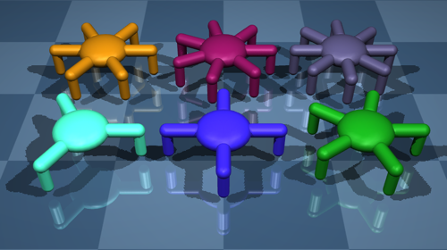
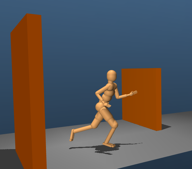
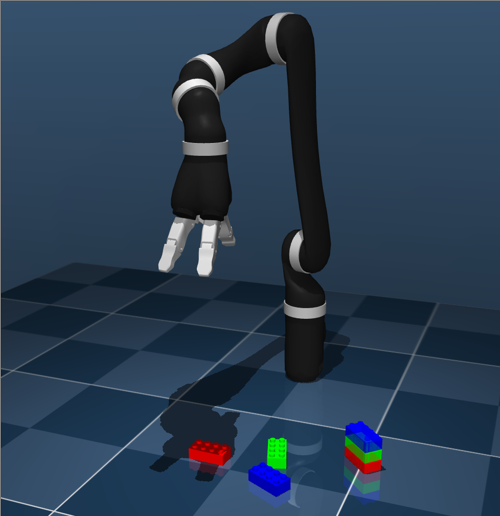
1 Introduction

Controlling the physical world is an integral part and arguably a prerequisite of general intelligence (Wolpert et al., 2003). Indeed, the only known example of general-purpose intelligence emerged in primates whose behavioural niche was already contingent on two-handed manipulation for millions of years.

Unlike board games, language and other symbolic domains, physical tasks are fundamentally continuous in state, time and action. Physical dynamics are subject to second-order equations of motion – the underlying state is composed of positions and velocities. Sensory signals (i.e. observations) carry meaningful physical units and vary over corresponding timescales. These properties, along with their prevalence and importance, make control problems a unique subset of general Markov Decision Processes. The most familiar physical control tasks have a fixed subset of degrees of freedom (the body) that are directly actuated, while the rest are unactuated (the environment). Such embodied tasks are the focus of dm_control.

1.1 Software for research

The dm_control package was designed by DeepMind scientists and engineers to facilitate their own continuous control and robotics needs, and is therefore well-suited for research. It is written in Python, exploiting the agile workflow of a dynamic language, while relying on the C-based MuJoCo physics library, a fast and accurate simulator (Erez et al., 2015), itself designed to facilitate research (Todorov et al., 2012). It is composed of the following modules:

• The ctypes-based MuJoCo wrapper (Sec. 2) provides full access to the simulator, conveniently exposing quantities with named indexing. A Python-based interactive visualiser (Sec. 2.2) allows the user to examine and perturb scene elements with a mouse.

• The PyMJCF library (Sec. 3) can procedurally assemble model elements and allows the user to configure or randomise parameters and initial states.

• An environment API that exposes actions, observations, rewards and terminations in a consistent yet flexible manner (Sec. 4).

• Finally, we combine the above functionality in the high-level task-definition framework Composer (Sec. 5). Amongst other things it provides a Model Variation module (Sec. 5.2) for policy robustification, and an Observable module for delayed, corrupted, and stacked sensor data (Sec. 5.1).

dm_control has been used extensively in DeepMind, serving as a fundamental component of continuous control research. See https://www.youtube.com/watch?v=CMjoiU482Jkyoutu.be/CMjoiU482Jk for a montage of clips from selected publications.

1.2 Tasks

Recent years have seen rapid progress in the application of Reinforcement Learning (RL) to difficult problem domains such as video games (Mnih, 2015). The Arcade Learning Environment (ALE, Bellemare et al. 2012) was and continues to be a vital facilitator of these developments, providing a set of standard benchmarks for evaluating and comparing learning algorithms. Similarly, it could be argued that control and robotics require well-designed task suites as a standardised playing field, where different approaches can compete and new ones can emerge.

The OpenAI Gym (Brockman et al., 2016) includes a set of continuous control domains that have become a popular benchmark in continuous RL (Duan et al., 2016; Henderson et al., 2017). More recent task suites such as Meta-world (Yu et al., 2019), SURREAL (Fan et al., 2018), RLbench (James et al., 2019) and IKEA (Lee et al., 2019), have been published in an attempt to satisfy the demand for tasks suites that facilitate the study of algorithms related to multi-scale control, multi-task transfer, and meta learning. dm_control includes its own sets of control tasks, in three categories:

Control Suite

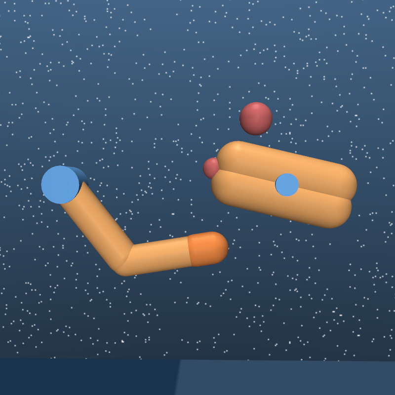
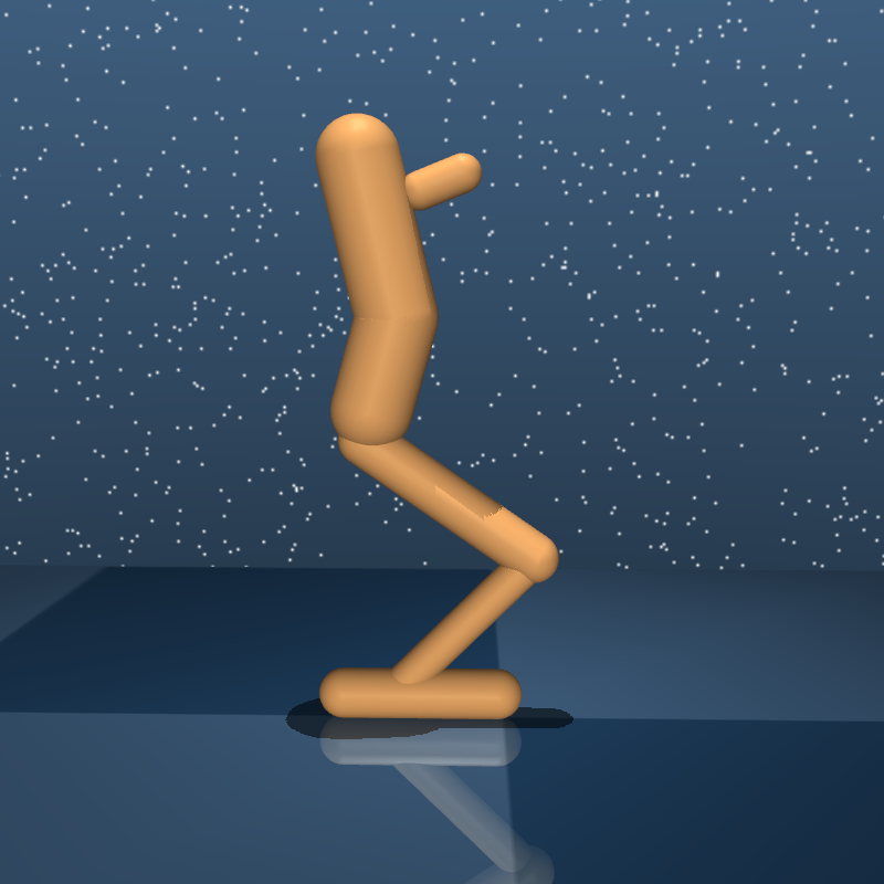
The DeepMind Control Suite (Section 6), first introduced in (Tassa et al., 2018), built directly with the MuJoCo wrapper, provides a set of standard benchmarks for continuous control problems. The unified reward structure offers interpretable learning curves and aggregated suite-wide performance measures. Furthermore, we emphasise high-quality, well-documented code using uniform design patterns, offering a readable, transparent and easily extensible codebase.

Locomotion

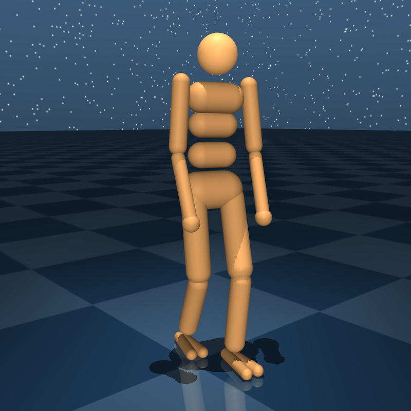
The Locomotion framework (Section 7) was inspired by our work in Heess et al. (2017). It is designed to facilitate the implementation of a wide range of locomotion tasks for RL algorithms by introducing self-contained, reusable components which compose into different task variants. The Locomotion framework has enabled a number of research efforts including Merel et al. (2017), Merel et al. (2019b), Merel et al. (2019a) and more recently has been employed to support Multi-Agent domains in Liu et al. (2019), Sunehag et al. (2019) and Banarse et al. (2019).

Manipulation

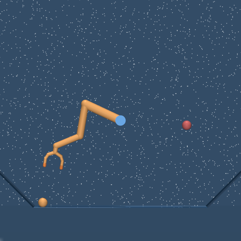
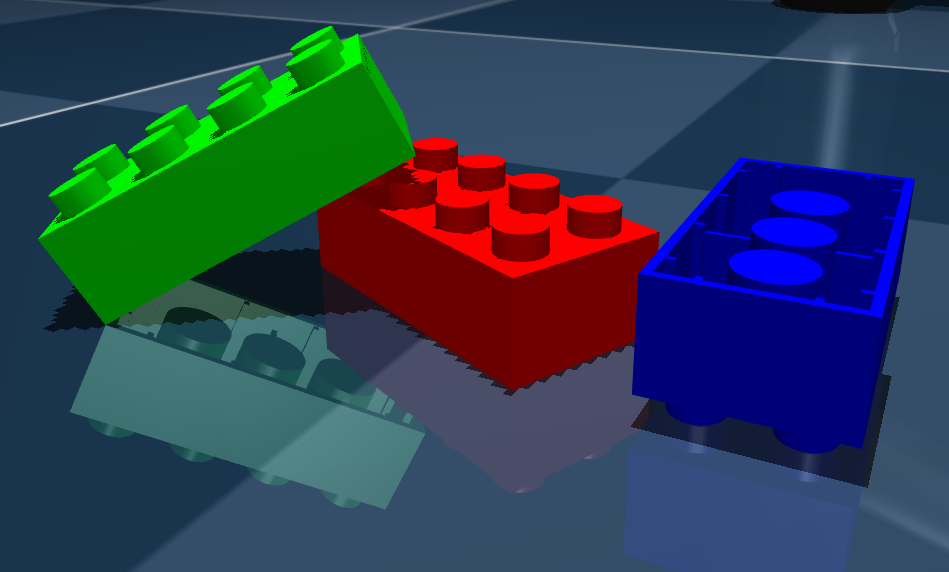
We also provide examples of constructing robotic manipulation tasks (Sec. 8). These tasks involve grabbing and manipulating objects with a 3D robotic arm. The set of tasks includes examples of reaching, placing, stacking, throwing, assembly and disassembly. The tasks are designed to be solved using a simulated 6 degree-of-freedom robotic arm based on the Kinova Jaco (Campeau-Lecours et al., 2017), though their modular design permit the use of other arms with minimal changes. These tasks make use of reusable components such as bricks that snap together, and provide examples of reward functions for manipulation. Tasks can be run using vision, low-level features, or combinations of both.

Part I Software Infrastructure

Sections 2, 3, 4 and 5 include code snippets showing how to use dm_control software. These snippets are collated in a Google Colab notebook:

https://colab.sandbox.google.com/github/deepmind/dm_control/blob/master/tutorial.ipynbgithub.com/deepmind/dm_control/tutorial.ipynb

2 MuJoCo Python interface

The mujoco module provides a general-purpose wrapper of the MuJoCo engine, using Python’s https://docs.python.org/3/library/ctypes.htmlctypes library to auto-generate bindings to MuJoCo structs, enums and API functions. We provide a brief introductory overview which assumes familiarity with Python; see in-code documentation for more detail.

MuJoCo physics

MuJoCo (Todorov et al., 2012) is a fast, reduced-coordinate, continuous-time physics engine. It compares favourably to other popular simulators (Erez et al., 2015), especially for articulated, low-to-medium degree-of-freedom regimes ($\lessapprox 100$) in the presence of contacts. The http://mujoco.org/book/modeling.htmlMJCF model definition format and reconfigurable computation pipeline have made MuJoCo a popular choice for robotics and reinforcement learning research (e.g. Schulman et al. 2015; Heess et al. 2015; Lillicrap et al. 2015; Duan et al. 2016).

2.1 The Physics class

The Physics class encapsulates MuJoCo’s most commonly used functionality.

Loading an MJCF model

The Physics.from_xml_string() constructor loads an MJCF model and returns a Physics instance:

⬇

from dm_control import mujoco

simple_MJCF = """

<mujoco>

<worldbody>

<light name="top" pos="0 0 1"/>

<body name="box_and_sphere" euler="0 0 -30">

<joint name="swing" type="hinge" axis="1 -1 0" pos="-.2 -.2 -.2"/>

<geom name="red_box" type="box" size=".2 .2 .2" rgba="1 0 0 1"/>

<geom name="green_sphere" pos=".2 .2 .2" size=".1" rgba="0 1 0 1"/>

</body>

</worldbody>

</mujoco>

"""

physics = mujoco.Physics.from_xml_string(simple_MJCF)

Rendering

The Physics.render() method outputs a NumPy array of pixel values.

⬇

pixels = physics.render()

[capbesideposition=right,top, capbesidewidth=0.65]figure[]

Optional arguments to render() specify the resolution, camera ID, whether to render RGB, depth or segmentation images, and other visualisation options (e.g. the joint visualisation on the left). dm_control on Linux supports both OSMesa software rendering and hardware-accelerated rendering using either EGL or GLFW. The rendering backend can be selected by setting the MUJOCO_GL environment variable to glfw, egl, or osmesa, respectively.

Physics.model and Physics.data

MuJoCo’s underlying mjModel and mjData data structures, describing static and dynamic simulation parameters respectively, can be accessed via the model and data properties of Physics. They contain NumPy arrays that have direct, writeable views onto MuJoCo’s internal memory. Because the memory is owned by MuJoCo, an attempt to overwrite an entire array throws an error:

⬇

# This fails with ‘AttributeError: can’t set attribute‘:

physics.data.qpos = np.random.randn(physics.model.nq)

# This succeeds:

physics.data.qpos[:] = np.random.randn(physics.model.nq)

mj_step() and Physics.step()

MuJoCo’s top-level mj_step() function computes the next state — the joint-space configuration qpos and velocity qvel — in two stages. Quantities that depend only on the state are computed in the first stage, mj_step1(), and those that also depend on the control (including forces) are computed in the subsequent mj_step2(). Physics.step() calls these sub-functions in reverse order, as follows. Assuming that mj_step1() has already been called, it first completes the computation of the new state with mj_step2(), and then calls mj_step1(), updating the quantities that depend on the state alone. In particular, this means that after a Physics.step(), rendered pixels will correspond to the current state, rather than the previous one. Quantities that depend on forces, like accelerometer and touch sensor readings, are still with respect to the last transition.

Setting the state with reset_context()

For the above assumption above to hold, mj_step1() must always be called after setting the state. We therefore provide the Physics.reset_context(), within which the state should be set:

⬇

with physics.reset_context():

# mj_reset() is called upon entering the context: default state.

physics.data.qpos[:] = ... # Set position.

physics.data.qvel[:] = ... # Set velocity.

# mj_forward() is called upon exiting the context. Now all derived

# quantities and sensor measurements are up-to-date.

Note that we call mj_forward() upon exit, which includes mj_step1(), but continues up to the computation of accelerations (but does not increment the state). This is so that force- or acceleration-dependent sensors have sensible values even at the initial state, before any steps have been taken.

Named indexing

Everything in a MuJoCo model can be named. It is often more convenient and less error-prone to refer to model elements by name rather than by index. To address this, Physics.named.model and Physics.named.data provide array-like containers that provide convenient named views. Using our simple model above:

⬇

print("The ‘geom_xpos‘ array:")

print(physics.data.geom_xpos)

print("Is much easier to inspect using ‘Physics.named‘:")

print(physics.named.data.geom_xpos)

⬇

The ‘geom_xpos‘ array:

[[0. 0. 0. ]

[0.27320508 0.07320508 0.2 ]]

Is much easier to inspect using ‘Physics.named‘:

x y z

0 red_box [ 0 0 0 ]

1 green_sphere [ 0.273 0.0732 0.2 ]

These containers can be indexed by name for both reading and writing, and support most forms of NumPy indexing:

⬇

with physics.reset_context():

physics.named.data.qpos[’swing’] = np.pi

print(physics.named.data.geom_xpos[’green_sphere’, [’z’]])

⬇

[-0.6]

Note that in the example above we use a joint name in order to index into the generalised position array qpos. Indexing into a multi-DoF ball or free joint outputs the appropriate slice. We also provide convenient access to MuJoCo’s mj_id2name and mj_name2id:

⬇

physics.model.id2name(0, "geom")

⬇

'red_box'

2.2 Interactive Viewer

The viewer module provides playback and interaction with physical models using mouse input. This type of visual debugging is often critical for cases when an agent finds an “exploit” in the physics.

⬇

from dm_control import suite, viewer

environment = suite.load(domain_name="humanoid", task_name="stand")

# Define a uniform random policy.

spec = environment.action_spec()

def random_policy(time_step):

return np.random.uniform(spec.minimum, spec.maximum, spec.shape)

# Launch the viewer application.

viewer.launch(environment, policy=random_policy)

See the documentation at https://github.com/deepmind/dm_control/tree/master/dm_control/viewerdm_control/tree/master/dm_control/viewer for a screen capture of the viewer application.

2.3 Wrapper bindings

The bindings provide easy access to all MuJoCo library functions and enums, automatically converting NumPy arrays to data pointers where appropriate.

⬇

from dm_control.mujoco.wrapper.mjbindings import mjlib

import numpy as np

quat = np.array((.5, .5, .5, .5))

mat = np.zeros(9)

mjlib.mju_quat2Mat(mat, quat)

print("MuJoCo converts this quaternion:")

print(quat)

print("To this rotation matrix:")

print(mat.reshape(3,3))

⬇

MuJoCo converts this quaternion:

[ 0.5 0.5 0.5 0.5]

To this rotation matrix:

[[ 0. 0. 1.]

[ 1. 0. 0.]

[ 0. 1. 0.]]

Enums are exposed as a submodule:

⬇

from dm_control.mujoco.wrapper.mjbindings import enums

print(enums.mjtJoint)

⬇

mjtJoint(mjJNT_FREE=0, mjJNT_BALL=1, mjJNT_SLIDE=2, mjJNT_HINGE=3)

3 The PyMJCF library

The PyMJCF library provides a Python object model for MuJoCo’s MJCF modelling language, which can describe complex scenes with articulated bodies. The goal of the library is to allow users to interact with and modify MJCF models programmatically using Python, similarly to what the JavaScript DOM does for HTML.

A key feature of the library is the ability to compose multiple MJCF models into a larger one, while automatically maintaining a consistent, collision-free namespace. Additionally, it provides Pythonic access to the underlying C data structures with the bind() method of mjcf.Physics, a subclass of Physics which associates a compiled model with the PyMJCF object tree.

3.1 PyMJCF Tutorial

The following code snippets constitute a tutorial example of a typical use case.

⬇

from dm_control import mjcf

class Leg(object):

""" A 2-DoF leg with position actuators."""

def __init__(self, length, rgba):

self.model = mjcf.RootElement()

# Defaults:

self.model.default.joint.damping = 2

self.model.default.joint.type = ’hinge’

self.model.default.geom.type = ’capsule’

self.model.default.geom.rgba = rgba # Continued below...

# Thigh:

self.thigh = self.model.worldbody.add(’body’)

self.hip = self.thigh.add(’joint’, axis=[0, 0, 1])

self.thigh.add(’geom’, fromto=[0, 0, 0, length, 0, 0], size=[length/4])

# Shin:

self.shin = self.thigh.add(’body’, pos=[length, 0, 0])

self.knee = self.shin.add(’joint’, axis=[0, 1, 0])

self.shin.add(’geom’, fromto=[0, 0, 0, 0, 0, -length], size=[length/5])

# Position actuators:

self.model.actuator.add(’position’, joint=self.hip, kp=10)

self.model.actuator.add(’position’, joint=self.knee, kp=10)

The Leg class describes an abstract articulated leg, with two joints and corresponding proportional-derivative actuators. Note the following.

• MJCF attributes correspond directly to arguments of the add() method.

• When referencing elements, e.g. when specifying the joint to which an actuator is attached in the last two lines above, the MJCF element itself can be used, rather than its name (though a name string is also supported).

⬇

BODY_RADIUS = 0.1

BODY_SIZE = (BODY_RADIUS, BODY_RADIUS, BODY_RADIUS / 2)

def make_creature(num_legs):

"""Constructs a creature with ‘num_legs‘ legs."""

rgba = np.random.uniform([0, 0, 0, 1], [1, 1, 1, 1])

model = mjcf.RootElement()

model.compiler.angle = ’radian’ # Use radians.

# Make the torso geom.

torso = model.worldbody.add(

’geom’, name=’torso’, type=’ellipsoid’, size=BODY_SIZE, rgba=rgba)

# Attach legs to equidistant sites on the circumference.

for i in range(num_legs):

theta = 2 * i * np.pi / num_legs

hip_pos = BODY_RADIUS * np.array([np.cos(theta), np.sin(theta), 0])

hip_site = model.worldbody.add(’site’, pos=hip_pos, euler=[0, 0, theta])

leg = Leg(length=BODY_RADIUS, rgba=rgba)

hip_site.attach(leg.model)

return model

The make_creature function uses PyMJCF’s attach() method to procedurally attach legs to the torso. Note that both the torso and hip attachment sites are children of the worldbody, since their parent body has yet to be instantiated. We will now make an arena with a chequered floor and two lights:

⬇

arena = mjcf.RootElement()

checker = arena.asset.add(’texture’, type=’2d’, builtin=’checker’, width=300,

height=300, rgb1=[.2, .3, .4], rgb2=[.3, .4, .5])

grid = arena.asset.add(’material’, name=’grid’, texture=checker,

texrepeat=[5,5], reflectance=.2)

arena.worldbody.add(’geom’, type=’plane’, size=[2, 2, .1], material=grid)

for x in [-2, 2]:

arena.worldbody.add(’light’, pos=[x, -1, 3], dir=[-x, 1, -2])

Placing several creatures in the arena, arranged in a grid:

⬇

# Instantiate 6 creatures with 3 to 8 legs.

creatures = [make_creature(num_legs=num_legs) for num_legs in (3,4,5,6,7,8)]

# Place them on a grid in the arena.

height = .15

grid = 5 * BODY_RADIUS

xpos, ypos, zpos = np.meshgrid([-grid, 0, grid], [0, grid], [height])

for i, model in enumerate(creatures):

# Place spawn sites on a grid.

spawn_pos = (xpos.flat[i], ypos.flat[i], zpos.flat[i])

spawn_site = arena.worldbody.add(’site’, pos=spawn_pos, group=3)

# Attach to the arena at the spawn sites, with a free joint.

spawn_site.attach(model).add(’freejoint’)

# Instantiate the physics and render.

physics = mjcf.Physics.from_mjcf_model(arena)

pixels = physics.render()

[capbesideposition=left,top, capbesidewidth=0.42]figure[]

Multi-legged creatures, ready to roam! Let us inject some controls and watch them move. We will generate a sinusoidal open-loop control signal of fixed frequency and random phase, recording both a video and the horizontal positions of the torso geoms, in order to plot the movement trajectories.

⬇

duration = 10 # (Seconds)

framerate = 30 # (Hz)

video = []; pos_x = []; pos_y = []

torsos = [] # List of torso geom elements.

actuators = [] # List of actuator elements.

for creature in creatures:

torsos.append(creature.find(’geom’,’torso’))

actuators.extend(creature.find_all(’actuator’))

# Control signal frequency, phase, amplitude.

freq = 5

phase = 2 * np.pi * np.random.rand(len(actuators))

amp = 0.9

# Simulate, saving video frames and torso locations.

physics.reset()

while physics.data.time < duration:

# Inject controls and step the physics.

physics.bind(actuators).ctrl = amp*np.sin(freq*physics.data.time + phase)

physics.step()

# Save torso horizontal positions using bind().

pos_x.append(physics.bind(torsos).xpos[:, 0].copy())

pos_y.append(physics.bind(torsos).xpos[:, 1].copy())

# Save video frames.

if len(video) < physics.data.time * framerate:

pixels = physics.render()

video.append(pixels.copy())

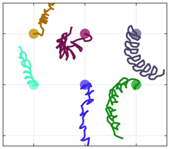
Plotting the movement trajectories, getting creature colours using bind():

⬇

creature_colors = physics.bind(torsos).rgba[:, :3]

fig, ax = plt.subplots(figsize=(8, 8))

ax.set_prop_cycle(color=creature_colors)

ax.plot(pos_x, pos_y, linewidth=4)

[capbesideposition=left,top, capbesidewidth=0.57]figure[]

https://youtu.be/0Lw_77PErjgyoutu.be/0Lw_77PErjg shows a clip of the locomotion. The plot on the right shows the corresponding movement trajectories of creature positions. Note how physics.bind(torsos) was used to access both xpos and rgba values. Once the Physics had been instantiated by from_mjcf_model(), the bind() method will expose both the associated mjData and mjModel fields of an mjcf element, providing unified access to all quantities in the simulation.

3.2 Debugging

In order to aid in troubleshooting MJCF compilation problems on models that are assembled programmatically, PyMJCF implements a debug mode where individual XML elements and attributes can be traced back to the line of Python code that last modified it. This feature is not enabled by default since the tracking mechanism is expensive to run. However when a compilation error is encountered the user is instructed to restart the program with the --pymjcf_debug runtime flag. This flag causes PyMJCF to internally log the Python stack trace each time the model is modified. MuJoCo’s error message is parsed to determine the line number in the generated XML document, which can be used to cross-reference to the XML element that is causing the error. The logged stack trace then allows PyMJCF to report the line of Python code that is likely to be responsible.

Occasionally, the XML compilation error arises from incompatibility between attached models or broken cross-references. Such errors are not necessarily local to the line of code that last modified a particular element. For such a scenario, PyMJCF provides an additional --pymjcf_debug_full_dump_dir flag that causes the entirety of the internal stack trace logs to be written to files at the specified directory.

4 Reinforcement learning interface

Reinforcement learning is a computational framework wherein an agent, through sequential interactions with an environment, tries to learn a behaviour policy that maximises future rewards (Sutton and Barto, 2018).

4.1 Reinforcement Learning API

Environments in dm_control adhere to DeepMind’s dm_env interface, defined in the https://github.com/deepmind/dm_envgithub.com/deepmind/dm_env repository. In brief, a run-loop using dm_env may look like

⬇

for _ in range(num_episodes):

timestep = env.reset()

while True:

action = agent.step(timestep)

timestep = env.step(action)

if timestep.last():

agent.step(timestep)

break

Each call to an environment’s step() method returns a TimeStep namedtuple with step_type, reward, discount and observation fields. Each episode starts with a step_type of FIRST, ends with a step_type of LAST, and has a step_type of MID for all intermediate timesteps. A TimeStep also has corresponding first(), mid() and last() methods, as illustrated above. Please see the dm_env https://github.com/deepmind/dm_env/blob/master/docs/index.mdrepository documentation for more details.

4.1.1 The Environment class

The class Environment, found within the dm_control.rl.control module, implements the dm_env environment interface:

reset()

Initialises the state, sampling from some initial state distribution.

step()

Accepts an action, advances the simulation by one time-step, and returns a TimeStep namedtuple.

action_spec()

describes the actions accepted by an Environment. The method returns an ArraySpec, with attributes that describe the shape, data type, and optional lower and upper bounds for the action arrays. For example, random agent interaction can be implemented as

⬇

spec = env.action_spec()

time_step = env.reset()

while not time_step.last():

action = np.random.uniform(spec.minimum, spec.maximum, spec.shape)

time_step = env.step(action)

observation_spec()

returns an OrderedDict of ArraySpecs describing the shape and data type of each corresponding observation.

A TimeStep namedtuple contains:

• step_type, an enum with a value in [FIRST, MID, LAST].

• reward, a floating point scalar, representing the reward from the previous transition.

• discount, a scalar floating point number $\gamma\in[0,1]$.

• observation, an OrderedDict of NumPy arrays matching the specification returned by observation_spec().

Whereas the step_type specifies whether or not the episode is terminating, it is the discount $\gamma$ that determines the termination type. $\gamma=0$ corresponds to a terminal state as in the first-exit or finite-horizon formulations. A terminal TimeStep with $\gamma=1$ corresponds to the infinite-horizon formulation; in this case an agent interacting with the environment should treat the episode as if it could have continued indefinitely, even though the sequence of observations and rewards is truncated. In this case a parametric value function may be used to estimate future returns.

4.2 Reward functions

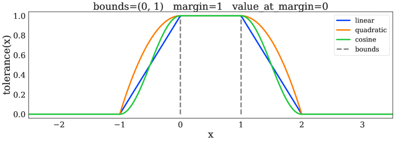
Rewards in dm_control tasks are in the unit interval, $r(\mathbf{s},\mathbf{a})\in[0,1]$. Some tasks have “sparse” rewards, i.e., $r(\mathbf{s},\mathbf{a})\in\{0,1\}$. This structure is facilitated by the tolerance() function, see Figure 3. Since terms output by tolerance() are in the unit interval, both averaging and multiplication operations maintain that property, facilitating reward design.

Figure 3: The tolerance(x, bounds=(lower, upper)) function returns 1 if x is within the bounds interval and 0 otherwise. If the optional margin argument is given, the output will decrease smoothly with distance from the interval, taking a value of value_at_margin at a distance of margin. Several types of sigmoid-like functions are available by setting the sigmoid argument. Top: Four infinite-support reward functions, for which value_at_margin must be positive. Bottom: Three finite-support reward functions with value_at_margin=0.

5 The Composer task definition library

The Composer framework organises RL environments into a common structure and endows scene elements with optional event handlers. At a high level, Composer defines three main abstractions for task design:

• composer.Entity represents a reusable self-contained building block that consists of an MJCF model, observables (Section 5.1), and possibly callbacks executed at specific stages of the environment’s life time, as detailed in Section 5.3. A collection of entities can be organised into a tree structure by attaching one or more child entities to a parent. The root entity is conventionally referred to as an “arena”, and provides a fixed <worldbody> for the final, combined MJCF model.

• composer.Task consists of a tree of composer.Entity objects that occupy the physical scene and provides reward, observation and termination methods. A task may also define callbacks to implement “game logic”, e.g. to modify the scene in response to various events, and provide additional task observables.

• composer.Environment wraps a composer.Task instance with an RL environment that agents can interact with. It is responsible for compiling the MJCF model, triggering callbacks at appropriate points of an episode (see Section 5.3), and determining when to terminate, either through task-defined termination criteria or a user defined time limit. It also holds a random number generator state that is used by the callbacks, enabling reproducibility.

Section 5.1 describes observable, a Composer module for exposing observations, supporting noise, buffering and delays. Section 5.2 describes variation, a module for implementing model variations. Section 5.3 describes the callbacks used by Composer to implement these and additional user-defined behaviours. A self-contained Composer tutorial follows in Section 5.4

5.1 The observableobservable module

An “observable” represents a quantity derived from the state of the simulation, that may be returned as an observation to the agent. Observables may be bound to a particular entity (e.g. sensors belonging to a robot), or they may be defined at the task level. The latter is often used for providing observations that relate to more than one entity in the scene (e.g. the distance between an end effector of a robot entity and a site on a different entity). A particular entity may define any number of observables (such as joint angles, pressure sensors, cameras), and it is up to the task designer to select which of these should appear in the agent’s observations. Observables can be configured in a number of ways:

• enabled: (boolean) Whether the observable is computed and returned to the agent. Set to False by default.

• update_interval: (integer or callable returning an integer) Specifies the interval, in simulation steps, at which the values of the observable will be updated. The last value will be repeated between updates. This parameter may be used to simulate sensors with different sample rates. Sensors with stochastic rates may be modelled by passing a callable that returns a random integer.

• buffer_size: (integer) Controls the size of the internal FIFO buffer used to store observations that were sampled on previous simulation time-steps. In the default case where no aggregator is provided (see below), the entire contents of the buffer is returned as an observation at each control timestep. This can be used to avoid discarding observations from sensors whose values may change significantly within the control timestep. If the buffer size is sufficiently large, it will contain observations from previous control timesteps, endowing the environment with a simple form of memory.

• corruptor: (callable) Performs a point-wise transformation of each observation value before it is inserted into the buffer. Corruptors are most commonly used to simulate observation noise.

• aggregator: (callable or predefined string) Performs a reduction over all of the elements in the observation buffer. For example this can be used to take a moving average over previous observation values.

• delay: (integer or callable returning an integer) Specifies a delay (in terms of simulation timesteps) between when the value of the observable is sampled, and when it will appear in the observations returned by the environment. This parameter can be used to model sensor latency. Stochastic latencies may be modelled by passing a callable that returns a randomly sampled integer.

During each control step the evaluation of observables is optimized such that only callables for observables that can appear in future observations are evaluated. For example, if we have an observable with update_interval=1 and buffer_size=1 then it will only be evaluated once per control step, even if there are multiple simulation steps per control step. This avoids the overhead of computing intermediate observations that would be discarded.

5.2 The variationvariation module

To improve the realism of the simulation, it is often desirable to randomise elements of the environment, especially those whose values are uncertain. Stochasticity can be added to both the observables e.g. sensor noise (the corruptor of the previous section), as well as the model itself (a.k.a. “domain randomisation”). The latter is a popular method for increasing the robustness learned control policies. The variation module provides methods to add and configure forms of stochasticity in the Composer framework. The following base API is provided:

• Variation: The base class. Subclasses should implement the abstract method __call__(self, initial_value, current_value, random_state),
  which returns a numerical value, possibly depending on an initial_value (e.g. original geom mass) and current_value (e.g. previously sampled geom mass). Variation objects support arithmetic operations with numerical primitives and other Variation objects.

• MJCFVariator: A class for varying attributes of MJCF elements, e.g. geom size. The MJCFVariator keeps track of initial and current attribute values and passes them to the Variation object. It should be called in the initialize_episode_mjcf stage, before the model is compiled.

• PhysicsVariator: Similar to MJCFVariator, except for bound attributes, e.g. external forces. Should be called in the initialize_episode stage after the model has been compiled.

• evaluate: Method to traverse an arbitrarily nested structure of callables or constant values, and evaluate any callables (such as Variation objects).

A number of submodules provide classes for commonly occurring use cases:

• colors: Used to define variations in different colour spaces, such as RGB, HSV and grayscale.

• deterministic: Deterministic variations such as constant and fixed sequences of values, in case more control over the exact values is required.

• distributions: Wraps a number of distributions available in numpy.random as Variation objects. Any distribution parameters passed can themselves also be Variation objects.

• noises: Used to define additive and multiplicative noise using the distributions mentioned above, e.g. for modelling sensor noise.

• rotations: Useful for defining variations in quaternion space, e.g. random rotation on a composer.Entity’s pose.

5.3 The Composer callback lifecycle

[0.9]

Figure 4: Diagram showing the life-cycle of Composer callbacks. Rounded rectangles represent callbacks that Tasks and Entities may implement. Blue rectangles represent built-in Composer operations.

Figure 4 illustrates the lifecycle of Composer callbacks. These can be organised into those that occur when an RL episode is reset, and those that occur when the environment is stepped. For a given callback, the one that is defined in the Task is executed first, followed by those defined in each Entity following depth-first traversal of the Entity tree starting from the root (which by convention is the arena) and the order in which Entities were attached.

The first of the two callbacks in reset is initialize_episode_mjcf, which allows the MJCF model to be modified between episodes. It is useful for changing quantities that are fixed once the model has been compiled. These modifications affect the generated XML which is then compiled into a Physics instance and passed to the initialize_episode callback, where the initial state can be set.

The Environment.step sequence begins at the before_step callback. One key role of this callback is to translate agent actions into the Physics control vector.

To guarantee stability, it is often necessary to reduce the time-step of the physics simulation. In order to decouple these possibly very small steps and the agent’s control time-step, we introduce a substep loop. Each Physics substep is preceded by before_substep and followed by after_substep. These callbacks are useful for detecting transient events that may occur in the middle of an environment step, e.g. a button press. The internal observation buffers are then updated according to the configured update_interval of each individual Observable, unless the substep happens to be the last one in the environment step, in which case the after_step callback is called first before the final update of the observation buffers. The internal observation buffers are then processed according to the delay, buffer_size, and aggregator settings of each Observable to generate “output buffers” that are returned externally.

At the end of each Environment.step, the Task’s get_reward, get_discount, and should_terminate_episode callbacks are called in order to obtain the step’s reward, discount, and termination status respectively. Usually, the these three are not entirely independent of each other, and it is therefore recommended to compute all of these in the after_step callback, cache the values in the Task instance, and return them in the respective callbacks.

5.4 Composer tutorial

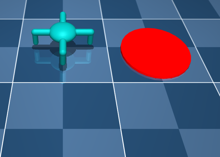
In this tutorial we will create a task requiring our “creature” from Section 3.1 to press a colour-changing button on the floor with a prescribed force. We begin by implementing our “creature” as a composer.Entity:

⬇

from dm_control import composer

from dm_control.composer.observation import observable

class Creature(composer.Entity):

"""A multi-legged creature derived from ‘composer.Entity‘."""

def _build(self, num_legs):

self._model = make_creature(num_legs)

def _build_observables(self):

return CreatureObservables(self)

@property

def mjcf_model(self):

return self._model

@property

def actuators(self):

return tuple(self._model.find_all(’actuator’))

class CreatureObservables(composer.Observables):

"""Add simple observable features for joint angles and velocities."""

@composer.observable

def joint_positions(self):

all_joints = self._entity.mjcf_model.find_all(’joint’)

return observable.MJCFFeature(’qpos’, all_joints)

@composer.observable

def joint_velocities(self):

all_joints = self._entity.mjcf_model.find_all(’joint’)

return observable.MJCFFeature(’qvel’, all_joints)

The Creature Entity includes generic Observables for joint angles and velocities. Because find_all() is called on the Creature’s MJCF model, it will only return the creature’s leg joints, and not the “free” joint with which it will be attached to the world. Note that Composer Entities should override the _build and _build_observables methods rather than __init__. The implementation of __init__ in the base class calls _build and _build_observables, in that order, to ensure that the entity’s MJCF model is created before its observables. This was a design choice which allows the user to refer to an observable as an attribute (entity.observables.foo) while still making it clear which attributes are observables. The stateful Button class derives from composer.Entity and implements the initialize_episode and after_substep callbacks.

⬇

NUM_SUBSTEPS = 25 # The number of physics substeps per control timestep.

class Button(composer.Entity):

"""A button Entity which changes colour when pressed with certain force."""

def _build(self, target_force_range=(5, 10)):

self._min_force, self._max_force = target_force_range

self._mjcf_model = mjcf.RootElement()

self._geom = self._mjcf_model.worldbody.add(

’geom’, type=’cylinder’, size=[0.25, 0.02], rgba=[1, 0, 0, 1])

self._site = self._mjcf_model.worldbody.add(

’site’, type=’cylinder’, size=self._geom.size*1.01, rgba=[1, 0, 0, 0])

self._sensor = self._mjcf_model.sensor.add(’touch’, site=self._site)

self._num_activated_steps = 0

def _build_observables(self):

return ButtonObservables(self)

@property

def mjcf_model(self):

return self._mjcf_model

def _update_activation(self, physics):

"""Update the activation and colour if the desired force is applied."""

current_force = physics.bind(self.touch_sensor).sensordata[0]

is_activated = (current_force >= self._min_force and

current_force <= self._max_force)

red = [1, 0, 0, 1]

green = [0, 1, 0, 1]

physics.bind(self._geom).rgba = green if is_activated else red

self._num_activated_steps += int(is_activated)

def initialize_episode(self, physics, random_state):

self._reward = 0.0

self._num_activated_steps = 0

self._update_activation(physics)

def after_substep(self, physics, random_state):

self._update_activation(physics)

@property

def touch_sensor(self):

return self._sensor

@property

def num_activated_steps(self):

return self._num_activated_steps

class ButtonObservables(composer.Observables):

"""A touch sensor which averages contact force over physics substeps."""

@composer.observable

def touch_force(self):

return observable.MJCFFeature(’sensordata’, self._entity.touch_sensor,

buffer_size=NUM_SUBSTEPS, aggregator=’mean’)

Note how the Button counts the number of sub-steps during which it is pressed with the desired force. It also exposes an Observable of the force being applied to the button, whose value is an average of the readings over the physics time-steps.

We import some variation modules and an arena factory (see Section 7):

⬇

from dm_control.composer import variation

from dm_control.composer.variation import distributions

from dm_control.composer.variation import noises

from dm_control.locomotion.arenas import floors

A simple Variation samples the initial position of the target:

⬇

class UniformCircle(variation.Variation):

""" A uniformly sampled horizontal point on a circle of radius ‘distance‘"""

def __init__(self, distance):

self._distance = distance

self._heading = distributions.Uniform(0, 2*np.pi)

def __call__(self, initial_value=None,

current_value=None, random_state=None):

distance, heading = variation.evaluate(

(self._distance, self._heading), random_state=random_state)

return (distance*np.cos(heading), distance*np.sin(heading), 0)

We will now define the PressWithSpecificForce Task, which combines all the above elements. The __init__ constructor sets up the scene:

⬇

class PressWithSpecificForce(composer.Task):

def __init__(self, creature):

self._creature = creature

self._arena = floors.Floor()

self._arena.add_free_entity(self._creature)

self._arena.mjcf_model.worldbody.add(’light’, pos=(0, 0, 4))

self._button = Button()

self._arena.attach(self._button)

# Configure initial poses

self._creature_initial_pose = (0, 0, 0.15)

button_distance = distributions.Uniform(0.5, .75)

self._button_initial_pose = UniformCircle(button_distance)

# Configure variators

self._mjcf_variator = variation.MJCFVariator()

self._physics_variator = variation.PhysicsVariator()

# Configure and enable observables

pos_corruptor = noises.Additive(distributions.Normal(scale=0.01))

self._creature.observables.joint_positions.corruptor = pos_corruptor

self._creature.observables.joint_positions.enabled = True

vel_corruptor = noises.Multiplicative(distributions.LogNormal(sigma=0.01))

self._creature.observables.joint_velocities.corruptor = vel_corruptor

self._creature.observables.joint_velocities.enabled = True

self._button.observables.touch_force.enabled = True

# Add button position observable in the Creature’s egocentric frame

self._task_observables = {}

def to_button(physics):

button_pos, _ = self._button.get_pose(physics)

return self._creature.global_vector_to_local_frame(physics, button_pos)

self._task_observables[’button_position’] = observable.Generic(to_button)

for obs in self._task_observables.values():

obs.enabled = True # Enable all observables.

self.control_timestep = NUM_SUBSTEPS * self.physics_timestep

# Continued below...

Continuing the PressWithSpecificForce Task definition, we now implement our Composer callbacks, including the reward function:

⬇

# Continued from above...

@property

def root_entity(self):

return self._arena

@property

def task_observables(self):

return self._task_observables

def initialize_episode_mjcf(self, random_state):

self._mjcf_variator.apply_variations(random_state)

def initialize_episode(self, physics, random_state):

self._physics_variator.apply_variations(physics, random_state)

creature_pose, button_pose = variation.evaluate(

(self._creature_initial_pose, self._button_initial_pose),

random_state=random_state)

self._creature.set_pose(physics, position=creature_pose)

self._button.set_pose(physics, position=button_pose)

def get_reward(self, physics):

return self._button.num_activated_steps / NUM_SUBSTEPS

Finally, we can instantiate a Creature Entity,

⬇

creature = Creature(num_legs=4)

pass it to the PressWithSpecificForce constructor to instantiate the task,

⬇

task = PressWithSpecificForce(creature)

and expose it as an environment complying with the dm_env.Environment API:

⬇

env = composer.Environment(task)

[capbesideposition=left,top, capbesidewidth=0.57]figure[]

Here is our creature with a large red button, waiting to be pressed.

Part II Tasks

6 The Control Suite

The Control Suite is a set of stable, well-tested tasks designed to serve as a benchmark for continuous control learning agents. Tasks are written using the basic MuJoCo interface of Section 2. Standardised action, observation and reward structures make suite-wide benchmarking simple and learning curves easy to interpret. Unlike the more elaborate domains of the Sections 7 and 8, Control Suite domains are not meant to be modified, in order to facilitate benchmarking. For more details regarding benchmarking, refer to our original publication (Tassa et al., 2018). A video montage of Control Suite domains can be found at https://www.youtube.com/watch?v=rAai4QzcYbsyoutu.be/rAai4QzcYbs.

6.1 Control Suite design conventions

Action:

With the exception of the LQR domain (see below), the action vector is in the unit box, i.e., $\mathbf{a}\in\mathcal{A}\equiv\left[-1,1\right]^{\dim(\mathcal{A})}$.

Dynamics:

While the state notionally evolves according to a continuous ordinary differential equation $\dot{\mathbf{s}}=\mathbf{f}_{c}(\mathbf{s},\mathbf{a})$, in practice temporal integration is discrete with some fixed, finite time-step: $\mathbf{s}_{t+h}=\mathbf{f}(\mathbf{s}_{t},\mathbf{a}_{t})$.

Observation:

When using the default observations (rather than pixels, see below), all tasks are strongly observable, i.e. the state can be recovered from a single observation. Observation features which depend only on the state (position and velocity) are functions of the current state. Features which are also dependent on controls (e.g. touch sensor readings) are functions of the previous transition.

Reward:

Rewards in the Control Suite, with the exception of the LQR domain, are in the unit interval, i.e., $r(\mathbf{s},\mathbf{a})\in[0,1]$. Some rewards are “sparse”, i.e., $r(\mathbf{s},\mathbf{a})\in\{0,1\}$. This structure is facilitated by the tolerance() function, see Figure 3.

Termination and Discount:

Control problems are usually classified as finite-horizon, first-exit and infinite-horizon (Bertsekas, 1995). Control Suite tasks have no terminal states or time limit and are therefore of the infinite-horizon variety. Notionally the objective is the infinite-horizon average return $\lim_{T\rightarrow\infty}T^{-1}\int_{0}^{T}r(\mathbf{s}_{t},\mathbf{a}_{t})dt$, but in practice our agents internally use the discounted formulation $\int_{0}^{\infty}e^{-t/\tau}r(\mathbf{s}_{t},\mathbf{a}_{t})dt$ or in discrete time $\sum_{i=0}^{\infty}\gamma^{i}r(\mathbf{s}_{i},\mathbf{a}_{i})$, where $\gamma=e^{-h/\tau}$ is the discount factor. In the limit $\tau\rightarrow\infty$ (equivalently $\gamma\rightarrow 1$), the policies of the discounted-horizon and average-return formulations are identical. All Control Suite tasks with the exception of LQR return $\gamma=1$ at every step, including on termination.

Evaluation:

While agents are expected to optimise for infinite-horizon returns, these are difficult to measure. As a proxy we use fixed-length episodes of 1000 time steps. Since all reward functions are designed so that $r\approx 1$ near goal states, learning curves measuring total returns can all have the same y-axis limits of $[0,1000]$, making them easier to interpret and to average over all tasks. While a perfect score of 1000 is not usually achievable, scores outside the $[800,1000]$ range can be confidently said to be sub-optimal.

Model and Task verification

Verification in this context means making sure that the physics simulation is stable and that the task is solvable:

• Simulated physics can easily destabilise and diverge, mostly due to errors introduced by time discretisation. Smaller time-steps are more stable, but require more computation per unit of simulation time, so the choice of time-step is always a trade-off between stability and speed (Erez et al., 2015). What’s more, learning agents are very good at discovering and exploiting instabilities.

• It is surprisingly easy to write tasks that are much easier or harder than intended, that are impossible to solve or that can be solved by very different strategies than expected (i.e. “cheats”). To prevent these situations, the Atari™ games that make up ALE were extensively tested over more than 10 man-years. However, many continuous control domains cannot be solved by humans with standard input devices, due to the large action space, so a different approach must be taken.

In order to tackle both of these challenges, we ran variety of learning agents (e.g. Lillicrap et al. 2015; Mnih et al. 2016) against all tasks, and iterated on each task’s design until we were satisfied that the physics was stable and non-exploitable, and that the task is solved correctly by at least one agent. Tasks that were solvable were collated into the benchmarking set. Tasks which were not yet solved at the time of development are in the extra set of tasks.

The suite module

To load an environment representing a task from the suite, use suite.load():

⬇

from dm_control import suite

# Load one task:

env = suite.load(domain_name="cartpole", task_name="swingup")

# Iterate over a task set:

for domain_name, task_name in suite.BENCHMARKING:

env = suite.load(domain_name, task_name)

...

Wrappers can be used to modify the behaviour of environments:

Pixel observations: By default, Control Suite environments return feature observations. The pixel.Wrapper adds or replaces these with images.

⬇

from dm_control.suite.wrappers import pixels

env = suite.load("cartpole", "swingup")

# Replace existing features by pixel observations:

env_only_pixels = pixels.Wrapper(env)

# Pixel observations in addition to existing features.

env_plus_pixels = pixels.Wrapper(env, pixels_only=False)

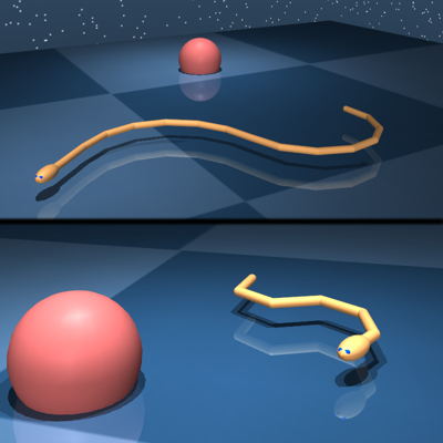
Reward visualisation: Models in the Control Suite use a common set of colours and textures for visual uniformity. As illustrated in the https://youtu.be/rAai4QzcYbsvideo, this also allows us to modify colours in proportion to the reward, providing a convenient visual cue.

⬇

env = suite.load("fish", "swim", task_kwargs, visualize_reward=True)

6.2 Domains and Tasks

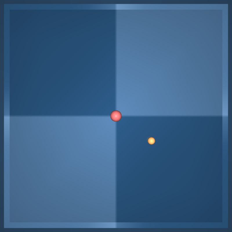
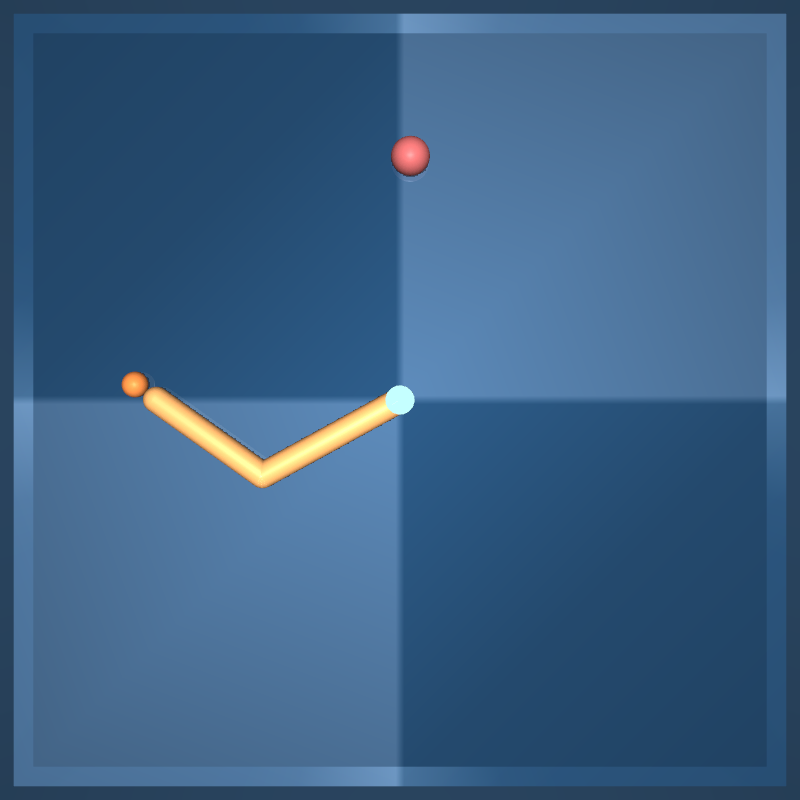
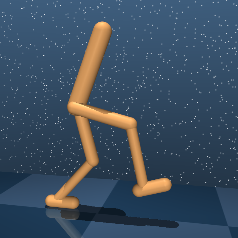
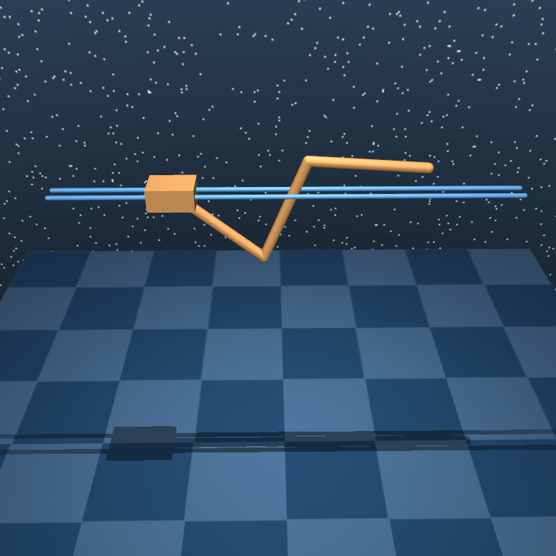
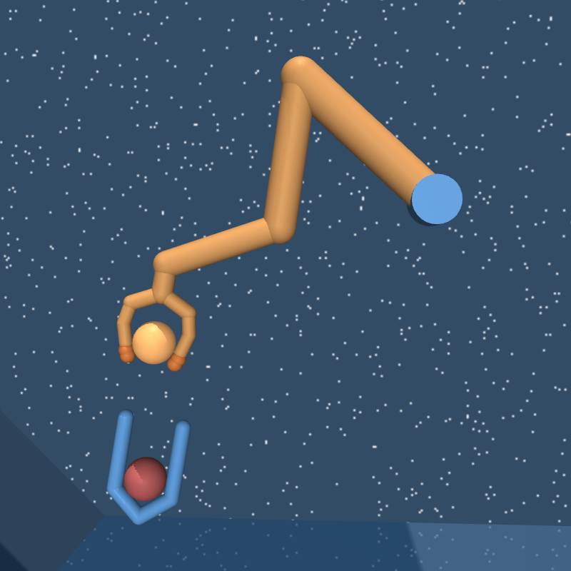
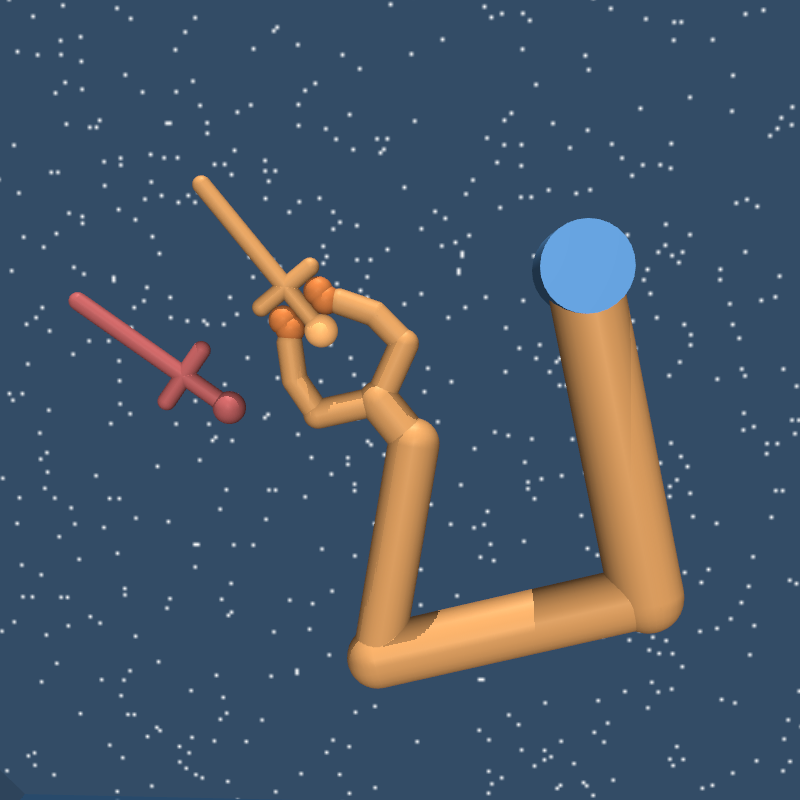
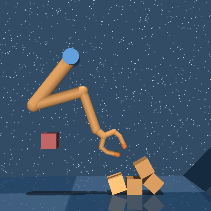
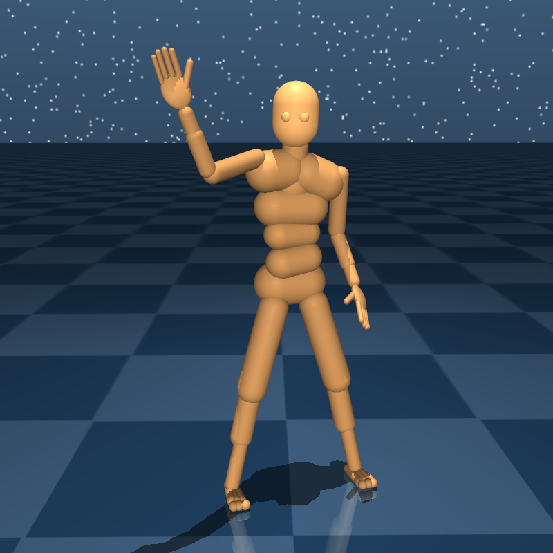
A domain refers to a physical model, while a task refers to an instance of that model with a particular MDP structure. For example the difference between the swingup and balance tasks of the cartpole domain is whether the pole is initialised pointing downwards or upwards, respectively. In some cases, e.g. when the model is procedurally generated, different tasks might have different physical properties. Tasks in the Control Suite are collated into tuples according to predefined tags. Tasks used for benchmarking are in the BENCHMARKING tuple (Figure 1), while those not used for benchmarking (because they are particularly difficult, or because they do not conform to the standard structure) are in the EXTRA tuple. All suite tasks are accessible via the ALL_TASKS tuple. In the domain descriptions below, names are followed by three integers specifying the dimensions of the state, control and observation spaces: $\textrm{\bf Name }\Bigl{(}\dim(\mathcal{S}),\dim(\mathcal{A}),\dim(\mathcal{O})\Bigr{)}$.

[capbesideposition=right,top, capbesidewidth=0.79]figure[]

Pendulum (2, 1, 3): The classic inverted pendulum. The torque-limited actuator is $1/6^{\mathrm{th}}$ as strong as required to lift the mass from motionless horizontal, necessitating several swings to swing up and balance. The swingup task has a simple sparse reward: 1 when the pole is within $30^{\circ}$ of the vertical position and 0 otherwise.

[capbesideposition=right,top, capbesidewidth=0.79]figure[]

Acrobot (4, 1, 6): The underactuated double pendulum, torque applied to the second joint. The goal is to swing up and balance. Despite being low-dimensional, this is not an easy control problem. The physical model conforms to (Coulom, 2002) rather than the earlier Spong 1995. The swingup and swingup_sparse tasks have smooth and sparse rewards, respectively.

[capbesideposition=right,top, capbesidewidth=0.79]figure[]

Cart-pole (4, 1, 5): Swing up and balance an unactuated pole by applying forces to a cart at its base. The physical model conforms to Barto et al. 1983. Four benchmarking tasks: in swingup and swingup_sparse the pole starts pointing down while in balance and balance_sparse the pole starts near the upright position.

[capbesideposition=right,top, capbesidewidth=0.585]figure[]  

Cart-k-pole ($\mathbf{2k\!+\!2,\;1,\;3k\!+\!2}$): The cart-pole domain allows to procedurally adding more poles, connected serially. Two non-benchmarking tasks, two_poles and three_poles are available.

[capbesideposition=right,top, capbesidewidth=0.79]figure[]

Ball in cup (8, 2, 8): A planar ball-in-cup task. An actuated planar receptacle can translate in the vertical plane in order to swing and catch a ball attached to its bottom. The catch task has a sparse reward: 1 when the ball is in the cup, 0 otherwise.

[capbesideposition=right,top, capbesidewidth=0.79]figure[]

Point-mass (4, 2, 4): A planar point mass receives a reward of 1 when within a target at the origin. In the easy task, one of simplest in the suite, the two actuators correspond to the global $x$ and $y$ axes. In the hard task, the gain matrix from the controls to the axes is randomised for each episode, making it impossible to solve by memoryless agents. This task is not in the benchmarking set.

[capbesideposition=right,top, capbesidewidth=0.79]figure[]

Reacher (4, 2, 6): The simple two-link planar reacher with a randomised target location. The reward is one when the end effector penetrates the target sphere. In the easy task the target sphere is bigger than on the hard task (shown on the left).

[capbesideposition=right,top, capbesidewidth=0.79]figure[]

Finger (6, 2, 12): A 3-DoF toy manipulation problem based on (Tassa and Todorov, 2010). A planar ‘finger’ is required to rotate a body on an unactuated hinge. In the turn_easy and turn_hard tasks, the tip of the free body must overlap with a target (the target is smaller for the turn_hard task). In the spin task, the body must be continually rotated.

[capbesideposition=right,top, capbesidewidth=0.79]figure[]

Hopper (14, 4, 15): The planar one-legged hopper introduced in (Lillicrap et al., 2015), initialised in a random configuration. In the stand task it is rewarded for bringing its torso to a minimal height. In the hop task it is rewarded for torso height and forward velocity.

[capbesideposition=right,top, capbesidewidth=0.79]figure[]

Fish (26, 5, 24): A fish is required to swim to a target. This domain relies on MuJoCo’s simplified fluid dynamics. There are two tasks: in the upright task, the fish is rewarded only for righting itself with respect to the vertical, while in the swim task it is also rewarded for swimming to the target.

[capbesideposition=right,top, capbesidewidth=0.79]figure[]

Cheetah (18, 6, 17): A running planar biped based on (Wawrzyński, 2009). The reward $r$ is linearly proportional to the forward velocity $v$ up to a maximum of $10\mathrm{m/s}$ i.e. $r(v)=\max\bigl{(}0,\min(v/10,1)\bigr{)}$.

[capbesideposition=right,top, capbesidewidth=0.79]figure[]

Walker (18, 6, 24): An improved planar walker based on the one introduced in (Lillicrap et al., 2015). In the stand task reward is a combination of terms encouraging an upright torso and some minimal torso height. The walk and run tasks include a component encouraging forward velocity.

[capbesideposition=right,top, capbesidewidth=0.79]figure[]

Manipulator (22, 5, 37): A planar manipulator is rewarded for bringing an object to a target location. In order to assist with exploration, in 10% of episodes the object is initialised in the gripper or at the target. Four manipulator tasks: {bring,insert}_{ball,peg} of which only bring_ball is in the benchmarking set. The other three are shown below.

[capbesideposition=right,top, capbesidewidth=0.415]figure[]

Manipulator extra: insert_ball: place the ball inside the basket. bring_peg: bring the peg to the target peg. insert_peg: insert the peg into the slot. See https://youtu.be/ESP-x6taBSwthis video for solutions of insertion tasks.

[capbesideposition=right,top, capbesidewidth=0.79]figure[]

Stacker ($\mathbf{6k\!+\!16,\;5,\;11k\!+\!26}$): Stack $k$ boxes. Reward is given when a box is at the target and the gripper is away from the target, making stacking necessary. The height of the target is sampled uniformly from $\{1,\ldots,k\}$.

[capbesideposition=right,top, capbesidewidth=0.79]figure[]

Swimmer ($\mathbf{2k\!+\!4,\;k\!-\!1,\;4k\!+\!1}$): This procedurally generated $k$-link planar swimmer is based on Coulom 2002, but using MuJoCo’s high-Reynolds fluid drag model. A reward of 1 is provided when the nose is inside the target and decreases smoothly with distance like a Lorentzian. The two instances provided in the benchmarking set are the 6-link and 15-link swimmers.

[capbesideposition=right,top, capbesidewidth=0.79]figure[]

Humanoid (54, 21, 67): A simplified humanoid with 21 joints, based on the model in (Tassa et al., 2012). Three tasks: stand, walk and run are differentiated by the desired horizontal speed of 0, 1 and $10\textrm{m/s}$, respectively. Observations are in an egocentric frame and many movement styles are possible solutions e.g. running backwards or sideways. This facilitates exploration of local optima.

[capbesideposition=right,top, capbesidewidth=0.79]figure[]

Humanoid_CMU (124, 56, 137): A humanoid body with 56 joints, adapted from (Merel et al., 2017) and based on the ASF model of subject #8 in the CMU Motion Capture Database. This domain has the same stand, walk and run tasks as the simpler humanoid. We include tools for parsing and playback of the CMU MoCap data, see below. A newer version of this model is now available; see Section 7.

[capbesideposition=right,top, capbesidewidth=0.79]figure[]

LQR (2n, m, 2n): $n$ masses, of which $m$ ($\leq n$) are actuated, move on linear joints which are connected serially. The reward is a quadratic in the position and controls. Analytic transition and control-gain matrices are derived and the optimal policy and value functions are computed in lqr_solver.py using Riccati iterations. Since both controls and reward are unbounded, LQR is not in the benchmarking set.

Control Suite Benchmarking

Please see the original tech report for the Control Suite (Tassa et al., 2018) for detailed benchmarking results of the BENCHMARKING tasks, with several popular Reinforcement Learning algorithms.

6.3 Additional domains

CMU Motion Capture Data

We enable humanoid_CMU to be used for imitation learning as in Merel et al. (2017), by providing tools for parsing, conversion and playback of human motion capture data from the CMU Motion Capture Database. The convert() function in the parse_amc module loads an AMC data file and returns a sequence of configurations for the humanoid_CMU model. The example script CMU_mocap_demo.py uses this function to generate a video.

Quadruped (56, 12, 58)

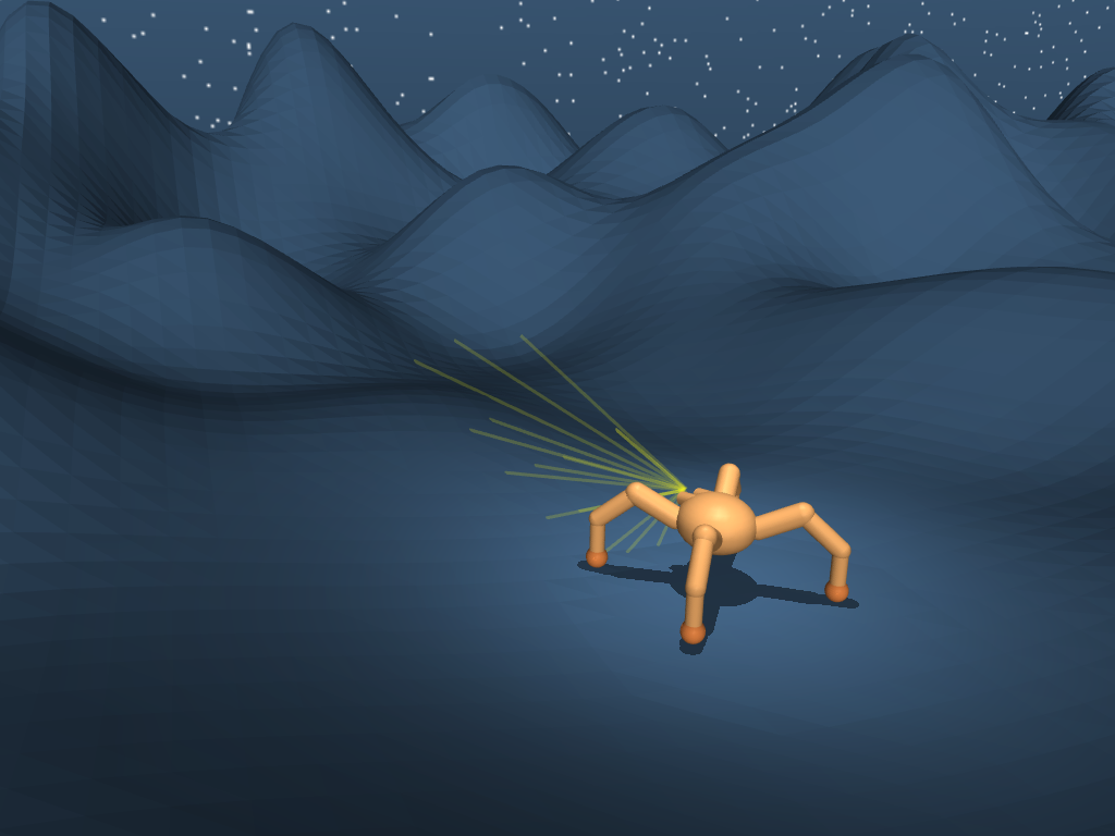
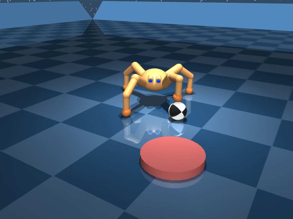
The quadruped (Figure 5) has 56 state dimensions. Each leg has 3 actuators for a total of 12 actions. Besides the basic walk and run tasks on flat ground, in the escape task the quadruped must climb over procedural random terrain using an array of 20 range-finder sensors (Figure 5, middle). In the fetch task (Figure 5, right), the quadruped must run after a moving ball and dribble it to a target at the centre of an enclosed arena. See solutions in https://youtu.be/RhRLjbb7pBEyoutu.be/RhRLjbb7pBE.

Figure 5: Left: The Quadruped. Middle: In the escape task the Quadruped must escape from random mountainous terrain using its rangefinder sensors. Right: In the fetch task the quadruped must fetch a moving ball and bring it to the red target.

Dog (158, 38, 227)

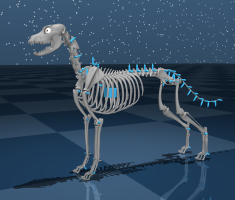
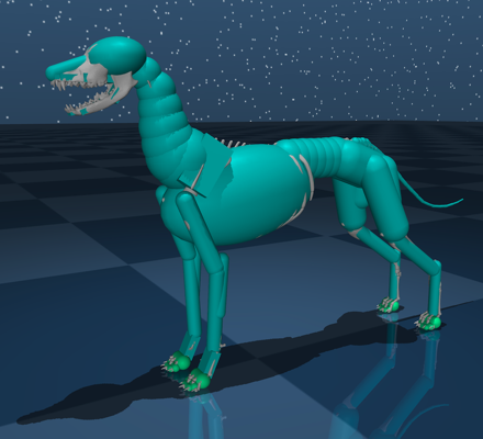
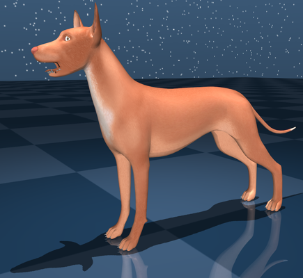
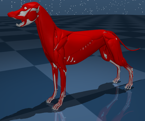
A realistic model of a Pharaoh Dog (Figure 6) was prepared for DeepMind by https://www.turbosquid.com/Search/Artists/leo3Dmodelsleo3Dmodels and is made available to the wider research community. The kinematics, skinning weights and collision geometry are created procedurally using PyMJCF. The static model includes muscles and tendon attachment points (Figure 6, Right). Including these in the dynamical model using MuJoCo’s support for tendons and muscles requires detailed anatomical knowledge and remains future work.

Figure 6: Left: Dog skeleton, joints visualised as light blue elements. Middle-Left: Collision geometry, overlain with skeleton. Middle-Right: Textured skin, used for visualisation only. Right: Dog muscles, included but not rigged to the skeleton. See https://youtu.be/i0_OjDil0Fgyoutu.be/i0_OjDil0Fg for preliminary solution of the run and fetch tasks.

Rodent (184, 38, 107 + 64$\times$64$\times$3 pixels)

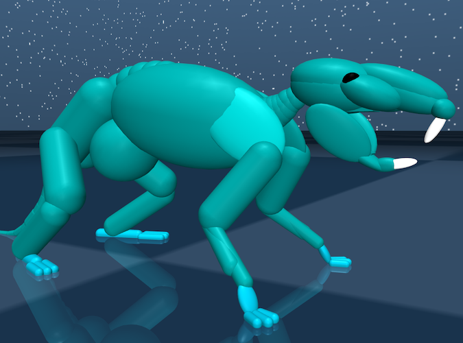
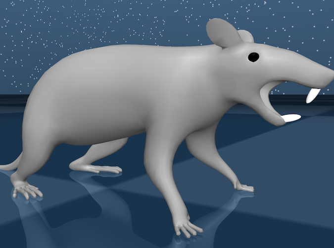
In order to better compare learned behaviour with experimental settings common in the life sciences, we have built a model of a rodent. See (Merel et al., 2020) for initial research training a policy to control this model using visual inputs and analysing the resulting neural representations. Related videos of rodent tasks therein: https://www.youtube.com/watch?v=vBIV1qJpJK8“forage”, https://www.youtube.com/watch?v=rFelC_YbeLE“gaps”, https://www.youtube.com/watch?v=6d0SX56Cn6Q“escape” and https://www.youtube.com/watch?v=lBKwHzO-z_0“two-tap”. The skeleton reference model was made by https://www.turbosquid.com/Search/Artists/leo3Dmodelsleo3Dmodels (not included).

Figure 7: Rodent; figure reproduced from Merel et al. 2020. Left: Anatomical skeleton of a rodent (as reference; not part of physical simulation). Middle-Left: Collision geometry designed around the skeleton. Middle-Right: Cosmetic skin to cover the body. Right: Semi-transparent visualisation of the three layers overlain.

7 Locomotion tasks

Inspired by our early work in Heess et al. 2017, the Locomotion library provides a framework and a set of high-level components for creating rich locomotion-related task domains. The central abstractions are the Walker, an agent-controlled Composer Entity that can move itself, and the Arena, the physical environment in which behaviour takes place. Walkers expose locomotion-specific methods, like observation transformations into an egocentric frame, while Arenas can re-scale themselves to fit Walkers of different sizes. Together with the Task, which includes a specification of episode initialisation, termination, and reward logic, a full RL environment is specified. The library currently includes navigating a corridor with obstacles, foraging for rewards in a maze, traversing rough terrain and multi-agent soccer. Many of these tasks were first introduced in Merel et al. 2019a and Liu et al. 2019.

7.1 Humanoid running along corridor with obstacles

Figure 8: A perspective of the environment in which the humanoid is tasked with navigating around walls along a corridor.

As an illustrative example of using the Locomotion infrastructure to build an RL environment, consider placing a humanoid in a corridor with walls, and a task specifying that the humanoid will be rewarded for running along this corridor, navigating around the wall obstacles using vision. We instantiate the environment as a composition of the Walker, Arena, and Task as follows. First, we build a position-controlled CMU humanoid walker.

⬇

walker = cmu_humanoid.CMUHumanoidPositionControlledV2020(

observable_options={’egocentric_camera’: dict(enabled=True)})

Note that this CMU humanoid is “V2020”, an improved version from the initial one released in Tassa et al. (2018). Modifications include overall body height and mass better matching a typical human, more realistic body proportions, and better tuned gains and torque limits for position-control actuators.

Next, we construct a corridor-shaped arena that is obstructed by walls.

⬇

arena = arenas.WallsCorridor(wall_gap=3.,

wall_width=distributions.Uniform(2., 3.),

wall_height=distributions.Uniform(2.5, 3.5),

corridor_width=4.,

corridor_length=30.)

Finally, a task that rewards the agent for running down the corridor at a specific velocity is instantiated as a composer.Environment.

⬇

task = tasks.RunThroughCorridor(walker=walker,

arena=arena,

walker_spawn_position=(0.5, 0, 0),

target_velocity=3.0,

physics_timestep=0.005,

control_timestep=0.03)

environment = composer.Environment(time_limit=10,

task=task,

strip_singleton_obs_buffer_dim=True)

https://youtu.be/UfSHdOg-bOAyoutu.be/UfSHdOg-bOA shows a video of a solution of this task, produced with Abdolmaleki et al. 2018’s MPO agent.

7.2 Maze navigation and foraging

[capbesideposition=left,top, capbesidewidth=0.57]figure[]

We include a procedural maze generator for arenas (the same one used in Beattie et al. 2016), to construct navigation and foraging tasks. On the right is the CMU humanoid in a human-sized maze, with spherical rewarding elements. https://www.youtube.com/watch?v=vBIV1qJpJK8youtu.be/vBIV1qJpJK8 shows the Rodent navigating a rodent-scale maze arena.

7.3 Multi-Agent soccer

Figure 9: Rendered scenes of Locomotion multi-agent soccer Left: 2-vs-2 with BoxHead walkers. Right: 3-vs-3 with Ant.

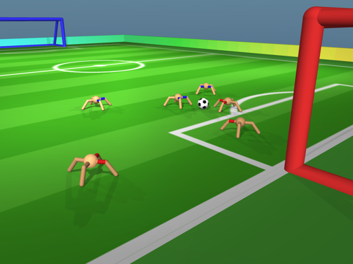
Building on Composer and Locomotion libraries, the Multi-agent soccer environments, introduced in Liu et al. 2019, follow a consistent task structure of Walkers, Arena, and Task where instead of a single walker, we inject multiple walkers that can interact with each other physically in the same scene. The code snippet below shows how to instantiate a 2-vs-2 Multi-agent Soccer environment with the simple, 5 degree-of-freedom BoxHead walker type. For example it can trivially be replaced by WalkerType.ANT, as shown in Figure 9.

⬇

from dm_control.locomotion import soccer

team_size = 2

num_walkers = 2 * team_size

env = soccer.load(team_size=team_size,

time_limit=45,

walker_type=soccer.WalkerType.BOXHEAD)

To implement a synchronous multi-agent environment, we adopt the convention that each TimeStep contains a sequence of per-agent observation dictionaries and expects a sequence of per-agent action arrays in return.

⬇

assert len(env.action_spec()) == num_walkers

assert len(env.observation_spec()) == num_walkers

# Reset and initialize the environment.

timestep = env.reset()

# Generates a random action according to the ‘action_spec‘.

random_actions = [spec.generate_value() for spec in env.action_spec()]

timestep = env.step(random_actions)

# Check that timestep respects multi-agent action and observation convention.

assert len(timestep.observation) == num_walkers

assert len(timestep.reward) == num_walkers

8 Manipulation tasks

Figure 10: Randomly sampled initial configurations for the lift_brick, place_cradle, and stack_3_bricks environments (left to right). The rightmost panel shows the corresponding 84x84 pixel visual observation returned by stack_3_bricks_vision. Note the stack of three translucent bricks to the right of the workspace, representing the goal configuration.

The manipulation module provides a robotic arm, a set of simple objects, and tools for building reward functions for manipulation tasks. Each example environment comes in two different versions that differ in the types of observation available to the agent:

1. features

   • Arm joint positions, velocities, and torques.

   • Task-specific privileged features (including the positions and velocities of other movable objects in the scene).

2. vision

   • Arm joint positions, velocities, and torques.

   • Fixed RGB camera view showing the workspace.

All of the manipulation environments return a reward $r(\mathbf{s},\mathbf{a})\in[0,1]$ per timestep, and have an episode time limit of 10 seconds. The following code snippet shows how to import the manipulation tasks and view all of the available environments:

⬇

from dm_control import manipulation

# ‘ALL‘ is a tuple containing the names of all of the environments.

print(’\n’.join(manipulation.ALL))

Environments are also tagged according to what types of observation they return. get_environments_by_tag lists the names of environments with specific tags:

⬇

print(’\n’.join(manipulation.get_environments_by_tag(’vision’)))

Environments are instantiated by name using the load method, which also takes an optional seed argument that can be used to seed the random number generator used by the environment.

⬇

env = manipulation.load(’stack_3_bricks_vision’, seed=42)

8.1 Studded brick model

[capbesideposition=left,top, capbesidewidth=0.67]figure[]

The stack_3_bricks_vision task, like most of the included manipulation tasks, makes use of the studded bricks shown on the right. These were modelled on Lego Duplo® bricks, snapping together when properly aligned and force is applied, and holding together using friction.

8.2 Task descriptions

Brief descriptions of each task are given below:

• reach_site: Move the end effector to a target location in 3D space.

• reach_brick: Move the end effector to a brick resting on the ground.

• lift_brick: Elevate a brick above a threshold height.

• lift_large_box: Elevate a large box above a threshold height. The box is too large to be grasped by the gripper, requiring non-prehensile manipulation.

• place_cradle: Place a brick inside a concave ‘cradle’ situated on a pedestal.

• place_brick: Place a brick on top of another brick that is attached to the top of a pedestal. Unlike the stacking tasks below, the two bricks are not required to be snapped together in order to obtain maximum reward.

• stack_2_bricks: Snap together two bricks, one of which is attached to the floor.

• stack_2_bricks_moveable_base: Same as stack_2_bricks, except both bricks are movable.

• stack_2_of_3_bricks_random_order: Same as stack_2_bricks, except there is a choice of two color-coded movable bricks, and the agent must place the correct one on top of the fixed bottom brick. The goal configuration is represented by a visual hint consisting of a stack of translucent, contactless bricks to the side of the workspace. In the features version of the task the observations also contain a vector of indices representing the desired order of the bricks.

• stack_3_bricks: Assemble a tower of 3 bricks. The bottom brick is attached to the floor, whereas the other two are movable. The top two bricks must be assembled in a specific order.

• stack_3_bricks_random_order: Same as stack_3_bricks, except the order of the top two bricks does not matter.

• reassemble_3_bricks_fixed_order: The episode begins with all three bricks already assembled in a stack, with the bottom brick being attached to the floor. The agent must disassemble the top two bricks in the stack, and reassemble them in the opposite order.

• reassemble_5_bricks_random_order: Same as the previous task, except there are 5 bricks in the initial stack. There are therefore $4!-1$ possible alternative configurations in which the top 4 bricks in the stack can be reassembled, of which only one is correct.

9 Conclusion

dm_control is a starting place for the testing and performance comparison of reinforcement learning algorithms for physics-based control. It offers a wide range of pre-designed RL tasks and a rich framework for designing new ones. We are excited to be sharing these tools with the wider community and hope that they will be found useful. We look forward to the diverse research the Control Suite and associated libraries may enable, and to integrating community contributions in future releases.

10 Acknowledgements

We would like to thank Raia Hadsell, Yori Zwols and Joseph Modayil for their reviews; Yazhe Li and Diego de Las Casas for their help with the Control Suite; Ali Eslami and Guy Lever for their contributions to the soccer environment.

References

- Abdolmaleki et al. (2018) Abbas Abdolmaleki, Jost Tobias Springenberg, Yuval Tassa, Rémi Munos, Nicolas Heess, and Martin A. Riedmiller. Maximum a posteriori policy optimisation. ICLR2018, abs/1806.06920, 2018.
- Banarse et al. (2019) Dylan Banarse, Yoram Bachrach, Siqi Liu, Guy Lever, Nicolas Heess, Chrisantha Fernando, Pushmeet Kohli, and Thore Graepel. The body is not a given: Joint agent policy learning and morphology evolution. In Proceedings of the 18th International Conference on Autonomous Agents and MultiAgent Systems, pages 1134–1142. International Foundation for Autonomous Agents and Multiagent Systems, 2019.
- Barto et al. (1983) A. G. Barto, R. S. Sutton, and C. W. Anderson. Neuronlike adaptive elements that can solve difficult learning control problems. IEEE Transactions on Systems, Man, and Cybernetics, SMC-13(5):834–846, Sept 1983. ISSN 0018-9472. doi: 10.1109/TSMC.1983.6313077.
- Beattie et al. (2016) Charles Beattie, Joel Z. Leibo, Denis Teplyashin, Tom Ward, Marcus Wainwright, Heinrich Küttler, Andrew Lefrancq, Simon Green, Víctor Valdés, Amir Sadik, Julian Schrittwieser, Keith Anderson, Sarah York, Max Cant, Adam Cain, Adrian Bolton, Stephen Gaffney, Helen King, Demis Hassabis, Shane Legg, and Stig Petersen. DeepMind Lab. arXiv e-prints, art. arXiv:1612.03801, December 2016.
- Bellemare et al. (2012) Marc G Bellemare, Yavar Naddaf, Joel Veness, and Michael Bowling. The arcade learning environment: An evaluation platform for general agents. Journal of Artificial Intelligence Research, 2012.
- Bertsekas (1995) Dimitri P Bertsekas. Dynamic programming and optimal control, volume 1. Athena scientific Belmont, MA, 1995.
- Brockman et al. (2016) Greg Brockman, Vicki Cheung, Ludwig Pettersson, Jonas Schneider, John Schulman, Jie Tang, and Wojciech Zaremba. Openai gym, 2016.
- Campeau-Lecours et al. (2017) Alexandre Campeau-Lecours, Hugo Lamontagne, Simon Latour, Philippe Fauteux, Véronique Maheu, François Boucher, Charles Deguire, and Louis-Joseph Caron L’Ecuyer. Kinova modular robot arms for service robotics applications. Int. J. Robot. Appl. Technol., 5(2):49–71, July 2017. ISSN 2166-7195.
- (9) CMU Graphics Lab. CMU Motion Capture Database. http://mocap.cs.cmu.edu, 2002. The database was created with funding from NSF EIA-0196217.
- Coulom (2002) Rémi Coulom. Reinforcement learning using neural networks, with applications to motor control. PhD thesis, Institut National Polytechnique de Grenoble-INPG, 2002.
- Duan et al. (2016) Yan Duan, Xi Chen, Rein Houthooft, John Schulman, and Pieter Abbeel. Benchmarking deep reinforcement learning for continuous control. In International Conference on Machine Learning, pages 1329–1338, 2016.
- Erez et al. (2015) Tom Erez, Yuval Tassa, and Emanuel Todorov. Simulation tools for model-based robotics: Comparison of bullet, havok, mujoco, ode and physx. In Robotics and Automation (ICRA), 2015 IEEE International Conference on, pages 4397–4404. IEEE, 2015.
- Fan et al. (2018) Linxi Fan, Yuke Zhu, Jiren Zhu, Zihua Liu, Orien Zeng, Anchit Gupta, Joan Creus-Costa, Silvio Savarese, and Li Fei-Fei. Surreal: Open-source reinforcement learning framework and robot manipulation benchmark. In Conference on Robot Learning, 2018.
- Heess et al. (2015) Nicolas Heess, Gregory Wayne, David Silver, Timothy Lillicrap, Tom Erez, and Yuval Tassa. Learning continuous control policies by stochastic value gradients. In C. Cortes, N. D. Lawrence, D. D. Lee, M. Sugiyama, and R. Garnett, editors, Advances in Neural Information Processing Systems 28, pages 2944–2952. Curran Associates, Inc., 2015.
- Heess et al. (2017) Nicolas Heess, Dhruva TB, Srinivasan Sriram, Jay Lemmon, Josh Merel, Greg Wayne, Yuval Tassa, Tom Erez, Ziyu Wang, S. M. Ali Eslami, Martin Riedmiller, and David Silver. Emergence of locomotion behaviours in rich environments, 2017.
- Henderson et al. (2017) Peter Henderson, Riashat Islam, Philip Bachman, Joelle Pineau, Doina Precup, and David Meger. Deep reinforcement learning that matters, 2017.
- James et al. (2019) Stephen James, Zicong Ma, David Rovick Arrojo, and Andrew J. Davison. RLBench: The Robot Learning Benchmark & Learning Environment. arXiv e-prints, art. arXiv:1909.12271, September 2019.
- Lee et al. (2019) Youngwoon Lee, Edward S Hu, Zhengyu Yang, Alex Yin, and Joseph J Lim. IKEA furniture assembly environment for long-horizon complex manipulation tasks. arXiv preprint arXiv:1911.07246, 2019. URL https://clvrai.com/furniture.
- Lillicrap et al. (2015) Timothy P Lillicrap, Jonathan J Hunt, Alexander Pritzel, Nicolas Heess, Tom Erez, Yuval Tassa, David Silver, and Daan Wierstra. Continuous control with deep reinforcement learning. arXiv preprint arXiv:1509.02971, 2015.
- Liu et al. (2019) Siqi Liu, Guy Lever, Josh Merel, Saran Tunyasuvunakool, Nicolas Heess, and Thore Graepel. Emergent coordination through competition. In International Conference on Learning Representations, 2019.
- Merel et al. (2017) Josh Merel, Yuval Tassa, TB Dhruva, Sriram Srinivasan, Jay Lemmon, Ziyu Wang, Greg Wayne, and Nicolas Heess. Learning human behaviors from motion capture by adversarial imitation. arXiv preprint arXiv:1707.02201, 2017.
- Merel et al. (2019a) Josh Merel, Arun Ahuja, Vu Pham, Saran Tunyasuvunakool, Siqi Liu, Dhruva Tirumala, Nicolas Heess, and Greg Wayne. Hierarchical visuomotor control of humanoids. In International Conference on Learning Representations, 2019a.
- Merel et al. (2019b) Josh Merel, Leonard Hasenclever, Alexandre Galashov, Arun Ahuja, Vu Pham, Greg Wayne, Yee Whye Teh, and Nicolas Heess. Neural probabilistic motor primitives for humanoid control. In International Conference on Learning Representations, 2019b.
- Merel et al. (2020) Josh Merel, Diego Aldarondo, Jesse Marshall, Yuval Tassa, Greg Wayne, and Bence Ölveczky. Deep neuroethology of a virtual rodent. In International Conference on Learning Representations, 2020.
- Mnih et al. (2016) Volodymyr Mnih, Adria Puigdomenech Badia, Mehdi Mirza, Alex Graves, Timothy P Lillicrap, Tim Harley, David Silver, and Koray Kavukcuoglu. Asynchronous methods for deep reinforcement learning. arXiv preprint arXiv:1602.01783, 2016.
- Mnih (2015) Volodymyr et al. Mnih. Human-level control through deep reinforcement learning. Nature, 518(7540):529–533, Feb 2015. ISSN 0028-0836. Letter.
- Schulman et al. (2015) John Schulman, Sergey Levine, Pieter Abbeel, Michael Jordan, and Philipp Moritz. Trust region policy optimization. In Proceedings of the 32nd International Conference on Machine Learning (ICML-15), pages 1889–1897, 2015.
- Sims (1994) Karl Sims. Evolving virtual creatures. In Proceedings of the 21st annual conference on Computer graphics and interactive techniques, pages 15–22. ACM, 1994.
- Spong (1995) Mark W Spong. The swing up control problem for the acrobot. IEEE control systems, 15(1):49–55, 1995.
- Sunehag et al. (2019) Peter Sunehag, Guy Lever, Siqi Liu, Josh Merel, Nicolas Heess, Joel Z. Leibo, Edward Hughes, Tom Eccles, and Thore Graepel. Reinforcement learning agents acquire flocking and symbiotic behaviour in simulated ecosystems. The 2019 Conference on Artificial Life, 1(31):103–110, 2019.
- Sutton and Barto (2018) Richard S. Sutton and Andrew G. Barto. Reinforcement Learning: An Introduction. The MIT Press, second edition, 2018. URL http://incompleteideas.net/book/the-book-2nd.html.
- Tassa and Todorov (2010) Yuval Tassa and Emo Todorov. Stochastic complementarity for local control of discontinuous dynamics. In Proceedings of Robotics: Science and Systems (RSS, 2010.
- Tassa et al. (2012) Yuval Tassa, Tom Erez, and Emanuel Todorov. Synthesis and stabilization of complex behaviors through online trajectory optimization. In Intelligent Robots and Systems (IROS), 2012 IEEE/RSJ International Conference on, pages 4906–4913. IEEE, 2012.
- Tassa et al. (2018) Yuval Tassa, Yotam Doron, Alistair Muldal, Tom Erez, Yazhe Li, Diego de Las Casas, David Budden, Abbas Abdolmaleki, Josh Merel, Andrew Lefrancq, Timothy Lillicrap, and Martin Riedmiller. DeepMind control suite. Technical report, DeepMind, January 2018. URL https://arxiv.org/abs/1801.00690.
- Todorov et al. (2012) Emanuel Todorov, Tom Erez, and Yuval Tassa. Mujoco: A physics engine for model-based control. In Intelligent Robots and Systems (IROS), 2012 IEEE/RSJ International Conference on, pages 5026–5033. IEEE, 2012.
- Wawrzyński (2009) Paweł Wawrzyński. Real-time reinforcement learning by sequential actor–critics and experience replay. Neural Networks, 22(10):1484–1497, 2009.
- Wolpert et al. (2003) Daniel Wolpert, Kenji Doya, and Mitsuo Kawato. A unifying computational framework for motor control and social interaction. Philosophical transactions of the Royal Society of London. Series B, Biological sciences, 358:593–602, 04 2003. doi: 10.1098/rstb.2002.1238.
- Yu et al. (2019) Tianhe Yu, Deirdre Quillen, Zhanpeng He, Ryan Julian, Karol Hausman, Chelsea Finn, and Sergey Levine. Meta-World: A Benchmark and Evaluation for Multi-Task and Meta Reinforcement Learning. arXiv e-prints, art. arXiv:1910.10897, October 2019.