Surrogate sea ice model enables
efficient tuning

Abstract

Predicting changes in sea ice cover is critical for shipping, ecosystem monitoring, and climate modeling. Current sea ice models, however, predict more ice than is observed in the Arctic, and less in the Antarctic. Improving the fit of these physics-based models to observations is challenging because the models are expensive to run, and therefore expensive to optimise. Here, we construct a machine learning surrogate that emulates the effect of changing model physics on forecasts of sea ice area from the Los Alamos Sea Ice Model (CICE). We use the surrogate model to investigate the sensitivity of CICE to changes in the parameters governing: ice’s ridging and albedo, snow’s albedo, aging, and thermal conductivity, the effect of meltwater on albedo, and the effect of ponds on albedo. We find that the CICE’s sensitivity to these model parameters differs between hemispheres. We propose that future sea ice modelers separate the snow conductivity and snow grain size distributions on a seasonal and inter-hemispheric basis, and we recommend optimal values of these parameters. This will make it possible to make models that fit observations of both Arctic and Antarctic sea ice more closely. These results demonstrate that important aspects of the behaviour of a leading sea ice model can be captured by a relatively simple support vector regression surrogate model, and that this surrogate dramatically increases the ease of tuning the full simulation.

1 Motivation

Understanding future sea ice extents is critical for naval and shipping strategies, conserving polar ecosystems, and modelling Earth’s energy balance and climate. Current models of sea ice, however, consistently predict more extensive Arctic sea ice than is observed (Stroeve et al., 2007; Perovich et al., 2019), and less extensive Antarctic sea ice (Eisenman et al., 2011; Stroeve & Meier, 2018). This misfit may be caused by missing or mis-calibrated model physics.

Sea ice models are designed to capture the physical processes that shape snow and ice on 10–30 km length scales, with smaller-scale processes represented through spatially averaged parameters (Hunke et al., 2017). The values of these parameters are tuned to observational data (Kim et al., 2006), but the tuning process is challenging, as each run of a global sea ice model can take days to weeks. Here, we develop a machine learning surrogate of the leading sea ice model, CICE (Hunke et al., 2017), use the surrogate model to efficiently evaluate the model’s response to changing parameters, demonstrate that the Arctic and Antarctic must be tuned separately, and provide recommendations for reducing the current model-data misfit.

2 Methods

Our model is designed to enable accelerated analysis and tuning of the Los Alamos Sea Ice Model, CICE. This is a global sea ice model used for operational ice forecasts, and its thermodynamic core is used in many sea ice and climate models worldwide. Thus, improving the accuracy of CICE is an effective route towards improving many widely-used sea ice forecasts. Although some authors have begun to use machine learning to predict the properties of current sea ice (Lee et al., 2016) machine learning is not yet integrated into operational forecasts.

Long-term sea ice trends are well-predicted by physics-based models. The cost of these models is high enough to make tuning inconvenient, but not so high as to warrant replacing the models entirely with ML systems. Therefore, we focus on making improvements to a widely-used model, rather than beginning from the ground up with a pure machine learning pipeline like Chi & Kim (2017). This approach allows us to leverage the speed of an ML emulator in the context where it is most effective, while retaining the predictive power of the physics-based model, and working within existing ice forecast infrastructure.

We sought a surrogate model that could capture the effect of selected model physics (§2.1) on CICE ice cover forecasts in realistic past atmospheric conditions (§2.2), with the goal of identifying strategies that simultaneously (1) decrease the model’s prediction of Arctic ice cover, (2) increase the prediction of Antarctic ice cover, and (3) improve the realism of the model physics.

2.1 Selection of target parameters

We selected seven CICE parameters that represent ice and snow processes with strong influences on total ice growth and area. These are listed in Table 1, along with their default values in CICE 4.0. The functions of these parameters are described fully in Hunke & Jeffery (2015). The parameter selection was guided by sensitivity studies of CICE (Urrego-Blanco et al., 2016; Blazey et al., 2013), which brought attention to the high degrees of uncertainty caused by parameterizations of snow and ice albedo (reflectivity), snow thermal conductivity, and snow aging.

Table 1: Parameters varied in CICE perturbed parameter ensemble.

Parameter		Range	Default
Snow thermal conductivity	ksno	0.10–0.35	0.30
Snow aging albedo parameter	r_snw	-1.9–1.9	1.5
Albedo adjustment from ice on snow	r_ice	-1.9–1.9	0.0
Albedo adjustment from ponds on snow	r_pnd	-1.9–1.9	0.0
Snow melt maximum radius	rsnw_melt_in	500–2000	1500
Melting onset temperature, ${}^{o}C$	dT_mlt_in	0.10–1.80	1.50
e-folding scale of ice ridges	mu_rdg	3.0–5.0	4

2.2 Data generation

From these parameters, we generated a perturbed parameter ensemble of 72 CICE simulations. Parameter combinations were selected using a Latin hypercube distribution, produced by the LLNL Uncertainty Quantification Pipeline (Brandon et al., 2011; Tannahill et al., 2011) within the ranges specified in Table 1.

To control the cost of generating this training data, we ran the ensemble with a repeated year 2000 atmospheric and ocean forcing. This is less realistic than a fully-coupled atmosphere that responds to changes in the sea ice, but tens of times faster. The atmosphere was modelled by the Community Atmosphere Model (CAM4, grid f19); the ocean as a slab ocean; the sea ice model used a displaced pole grid (gx1v6); and the land surfaces using the Community Land Model (Oleson et al., 2010). The simulations ran for 40 years, the first 30 of which were used to spin up the model. To average out the internal variability of the climate, we averaged the last 10 years of the runs together.

2.3 Surrogate model design

The surrogate model predicts ice area and extent as a function of seven CICE model parameters (r_snw, r_pnd, r_ice, dt_melt_in, rsnw_melt_in, ksno and mu_rdg) and a specific query (ice area or extent, in either the northern or southern hemisphere, in a specific month). The surrogate model is a support vector regression (Smola & Scholkopf, 2004), implemented in Python using scikit-learn (Pedregosa et al., 2011).

2.4 Testing and validation

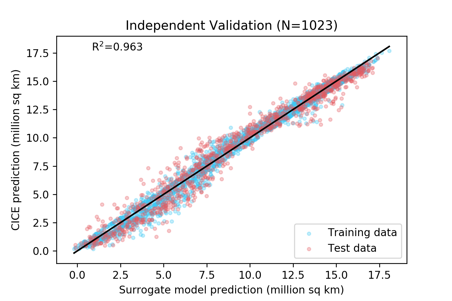
The model was trained and tested on 3360 data points (each representing ice area or extent, in a given month, in a given hemisphere, for one of the 72 members of the perturbed parameter ensemble). We split test and training data randomly at a ratio of 3:7. The model is not particularly sensitive to the test/training data split: a fifteen-fold cross-validation with random splits returned R² goodness of fit scores varying between 0.952–0.968. The model used in the final study (Fig. 1) has a typical value of R²=0.963.

Figure 1: Surrogate model tuning and validation. Left: Fit between tuned surrogate model output and CICE output. Right: Variation in surrogate model fit as a function of hyperparameters $C$ and $\gamma$ for fixed $\nu=0.45$. Lighter colors represent better fits.

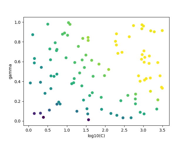
Our SVR model’s behavior is governed by a set of hyperparameters: $C$, $\gamma$, and $\nu$. We tuned the model by searching this hyperparameter space for the best fit (Fig. 1b). We settled on $C=318$, $\gamma=0.868$, and $\nu=0.349$ to balance surrogate model speed (which decreases with $C$) and accuracy, and used these values for the remainder of the study.

2.5 Bayesian calculation of model-data fit

We compare the CICE model results to observed data from the NSIDC sea ice index (Fetterer et al., 2017). Both modelled and observed data consist of monthly averages of ice area and extent in 2000. The difference between our model and the observations is its misfit. Misfit approaches zero as the model–data fit becomes perfect (or, as the likelihood that the observed data was produced by that model becomes high), is negative if the model predicts less ice than was observed, and is positive if the model predicts more ice than was observed. The misfit is given by

$$\mathrm{misfit}(\vec{\theta})=\left(M_{0}\right)\left(\vec{x}(\vec{\theta})-\vec{y}\right)\left({\mathrm{cov}}^{-1}\right)\left(\vec{x}(\vec{\theta})-\vec{y}\right)$$ (1)

where $\vec{\theta}$ is a set of parameters, $\vec{y}$ is observational data, $\vec{x}$ is model data, $\mathrm{{cov}}^{-1}$ is the inverse covariance matrix for the observational data, and $M_{0}$ is a normalization constant such that the misfit for the default parameter settings (Table 1) has magnitude 1.

The magnitude of the $\mathrm{misfit}$ is inversely related to the posterior probability, $p(\vec{\theta}|\vec{y})$, that known observations $\vec{y}$ could be produced by a model with parameters $\vec{\theta}$, assuming a uniform prior probability for those parameters. Thus, the set of parameters that minimizes the absolute value of the misfit has the highest likelihood of reproducing the observational data.

3 Results

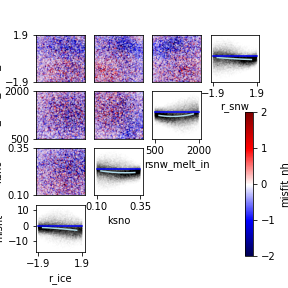
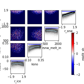
The surrogate model is dramatically faster than CICE: each data point for ice area and extent is generated in $\sim$5 ms, versus $\sim$96 CPU hours for each of the model runs described above — about $7\times 10^{7}$ times faster. This made it possible to explore the model’s behavior through a Monte-Carlo study of 600,000 parameter combinations. The resulting model–data misfits are shown for selected parameters in Fig. 2.

Figure 2: Likelihood that different sea ice model (CICE) parameterizations would have reproduced observed ice area and extent in year 2000. Left: probability of producing Arctic observations. Right: probability of producing Antarctic observations. Colored plots are bivariate distributions, white background plots are univariate distributions with trend lines. Blue indicates that the model produces less ice than is observed whereas red indicates that the model produces excess ice; white indicates good agreement.

These results reveal that Arctic and Antarctic sea ice respond differently to changes in model parameters. Specifically, the parameter range we explored contains many good fits to the Arctic data (white dots in Fig. 2 left), but most of those parameter combinations produce far too little ice (blue) in the Antarctic (Fig. 2 right). Moreover, the two hemispheres have opposite sensitivities to some parameters: increasing r_snw or ksno strongly increases the ice cover in the Antarctic, but not in the Arctic.

4 Implications for sea ice model design

We find that the effects of sea ice parameters on predicted ice cover differ between the Arctic and Antarctic. We recommend that sea ice model developers treat parameters such as ksno and r_snw not as global parameters, but as dynamic properties that may change in space or time. Specifically, as a simple, high-level fix, we recommend that developers use a lower value of the thermal conductivity of snow, ksno, in the Antarctic than the Arctic, and a higher value of the snow aging parameter r_snw. Implementing this change could quickly create models that better fit observations of Antarctic sea ice, and would add physical realism: both the thermal conductivity and the effect of aging on snow differ between the hemispheres (Sturm et al., 2002; Massom et al., 2001).

In future work, we intend to validate this recommendation by implementing it within CICE, and exploring the effect of improved sea ice model parameters on the global energy balance. We have also limited this discussion to variations of the largest possible scale. In future work, we intend to explore the effect of these model parameters on regional and seasonal sea ice variability, as well as the inter-hemisphere variability explored here. Field studies have shown that the physics of sea ice is variable on many scales, ranging from regional differences in snowfall and wind speed (Holland & Kwok, 2012), to meter-scale variability in the form of ice leads or snow dunes (Popović et al., 2018; Kochanski et al., 2018).

This study shows that the behaviours of the leading sea ice model CICE can be captured by a relatively simple support vector regression surrogate model and that this surrogate dramatically increases the ease of exploring the behaviours of the full simulation. This facilitates better decisions about the structure of the physics-based model.

References

- Blazey et al. (2013) B A Blazey, M M Holland, and E C Hunke. The Cryosphere Arctic Ocean sea ice snow depth evaluation and bias sensitivity in CCSM. The Cryosphere, 7:1887–1900, 2013. doi: 10.5194/tc-7-1887-2013.
- Brandon et al. (2011) S. Brandon, D. Domyancic, J. Tannahill, D. Lucas, G. Christianson, J. McEnereny, and R. Klein. Ensemble calculation via the LLNL uq pipeline: A user’s guide. Technical report, Tech. Rep. LLNL-SM-480999, 2011.
- Chi & Kim (2017) Junhwa Chi and Hyun Choel Kim. Prediction of Arctic sea ice concentration using a fully data driven deep neural network. Remote Sensing, 9(12), 2017. ISSN 20724292. doi: 10.3390/rs9121305.
- Eisenman et al. (2011) Ian Eisenman, Tapio Schneider, David S. Battisti, and Cecilia M. Bitz. Consistent changes in the sea ice seasonal cycle in response to global warming. Journal of Climate, 24(20):5325–5335, 2011. ISSN 08948755. doi: 10.1175/2011JCLI4051.1.
- Fetterer et al. (2017) F Fetterer, K Knowles, W N Meier, M Savole, and A K Windnagel. Sea Ice Index, Version 3. Technical report, Boulder, Colorado, USA, 2017.
- Holland & Kwok (2012) P R Holland and Ron Kwok. Wind-driven trends in Antarctic sea-ice drift. Nature Geoscience2, 5(12):872–875, 2012.
- Hunke & Jeffery (2015) E Hunke and N Jeffery. Snow-on-Sea-Ice Model for CICE and MPAS-CICE Requirements and Design. 2015.
- Hunke et al. (2017) E Hunke, W Lipscomb, P Jones, A Turner, and N Jeffery. CICE, The Los Alamos Sea Ice Model, Version 00, 2017. URL https://www.osti.gov//servlets/purl/1364126.
- Kim et al. (2006) J Kim, E Hunke, and W Lipscomb. Sensitivity analysis and parameter tuning scheme for global sea-ice modeling. Ocean modelling, 14((1-2)):61–80, 2006.
- Kochanski et al. (2018) K Kochanski, G Tucker, and R S Anderson. Statistical classification of self-organized snow surfaces. Geophysical Research Letters, 45:6532–6541, 2018. doi: 10.1029/2018GL077616.
- Lee et al. (2016) Sanggyun Lee, Jungho Im, Jinwoo Kim, Miae Kim, Minso Shin, Hyun cheol Kim, and Lindi J. Quackenbush. Arctic Sea Ice Thickness Estimation from CryoSat-2 Satellite Data Using Machine Learning-Based Lead Detection. Remote Sensing, 8(9), 2016. ISSN 20724292. doi: 10.3390/rs8090698.
- Massom et al. (2001) Robert A. Massom, Hajo Eicken, Christian Haas, Martin O. Jeffries, Mark R. Drinkwater, Matthew Sturm, Anthony P. Worby, Xingren Wu, Victoria I. Lytle, Shuki Ushio, Kim Morris, Phillip A. Reid, Stephen G. Warren, and Ian Allison. Snow on Antarctic sea ice. Reviews of Geophysics, 39(3):413–445, 2001. ISSN 87551209. doi: 10.1029/2000RG000085.
- Oleson et al. (2010) Keith W. Oleson, David M. Lawrence, Gordon B, Mark G. Flanner, Erik Kluzek, Peter J, Samuel Levis, Sean C. Swenson, E. Thornton, Johannes Feddema, Colette L. Heald, Jean-francois Lamarque, Guo-yue Niu, Taotao Qian, Steve Running, Koichi Sakaguchi, Liang Yang, Xiaodong Zeng, Xubin Zeng, and Mark Decker. Technical description of version 4.0 of the Community Land Model (CLM). Technical report, 2010.
- Pedregosa et al. (2011) F Pedregosa, G Varoquaux, A Gramfort, V Michel, B Thirion, O Grisel, M Blondel, P Prettenhofer, R Weiss, V Dubourg, J Vanderplas, A Passos, D Cournapeau, M Brucher, M Perrot, and E Duchesnay. Scikit-learn: Machine learning in Python. Journal of Machine Learning Research, 12:2825–2830, 2011.
- Perovich et al. (2019) D Perovich, W Meier, M Tschudi, S Farrell, S Hendricks, S Gerland, L Kaleschke, R Ricker, X Tian-Kunze, M Webster, and K Wood. Sea ice. In J Richter-Menge, M L Druckenmiller, and M Jeffries (eds.), 2019 Arctic Report Card. NOAA, Boulder, CO, USA, 2019.
- Popović et al. (2018) P Popović, B B Cael, M Silber, and D S Abbot. Simple rules govern the patterns of Arctic sea ice melt ponds. Physical Review Letters2, 120(4):148701, 2018.
- Smola & Scholkopf (2004) Alex J Smola and Bernhard Scholkopf. A tutorial on support vector regression. Statistics and Computing, 14:199–222, 2004. ISSN 0960-3174. doi: 10.1023/B:STCO.0000035301.49549.88.
- Stroeve & Meier (2018) J Stroeve and W N Meier. Sea Ice Trends and Climatologies from SSMR and SSM/I-SSMIS, Version 3. Technical report, NASA National Snow and Ice Data Center, Boulder, CO, USA, 2018.
- Stroeve et al. (2007) J Stroeve, M Holland, W Meier, T Scambos, and M Serreze. Arctic sea ice decline: Faster than forecast. Geophysical Research Letters, 34(9), 2007.
- Sturm et al. (2002) Matthew Sturm, Donald K Perovich, and Jon Holmgren. Thermal conductivity and heat transfer through the snow on the ice of the Beaufort Sea. Journal of Geophysical Research, 107(C10):8043, 2002. ISSN 0148-0227. doi: 10.1029/2000JC000409. URL http://doi.wiley.com/10.1029/2000JC000409.
- Tannahill et al. (2011) J Tannahill, D Lucas, D Domyancic, S Brandon, and R Klein. Data intensive uncertainty quantification: applications to climate modeling. Proceedings of the 2011 High Performance Computing Networking Storage and Analysis Conference, 2011.
- Urrego-Blanco et al. (2016) Jorge R. Urrego-Blanco, Nathan M. Urban, Elizabeth C. Hunke, Adrian K. Turner, and Nicole Jeffery. Uncertainty quantification and global sensitivity analysis of the Los Alamos sea ice model. Journal of Geophysical Research: Oceans, 121(4):2709–2732, 2016. ISSN 21699291. doi: 10.1002/2015JC011558.