The unbearable lightness of equilibria in a low interest rate environment

Abstract

Structural models with no solution are incoherent, and those with multiple solutions are incomplete. We show that models with occasionally binding constraints are not generically coherent. Coherency requires restrictions on the parameters or on the support of the distribution of the shocks. In presence of multiple shocks, the support restrictions cannot be independent from each other, so the assumption of orthogonality of structural shocks is incompatible with coherency. Models whose coherency is based on support restrictions are generically incomplete, admitting a very large number of minimum state variable solutions.

Keywords: incompleteness, incoherency, rational expectations, zero lower bound, DSGE

JEL codes: C62, E4, E52

1 Introduction

It is well-known that in structural models with occasionally binding constraints, equilibria may not exist (incoherency) or there may be multiple equilibria (incompleteness). Gourieroux et al. (1980) (henceforth GLM) studied this problem in the context of simultaneous equations models with endogenous regime switching, and derived conditions for existence and uniqueness of solutions, which are known as ‘coherency and completeness’ (CC) conditions. Aruoba et al. (2021b) and Mavroeidis (2021) derived these conditions for structural vector autoregressions with occasionally binding constraints. However, to the best of our knowledge, there are no general results about the conditions for existence and uniqueness of equilibria in dynamic forward-looking models with rational expectations when some variables are subject to occasionally binding constraints. This is despite the fact that there is a large and expanding literature on solution algorithms for such models (see Fernández-Villaverde et al., 2016) applied for example to models with a zero lower bound (ZLB) constraint on the interest rate (see e.g., Fernández-Villaverde et al., 2015; Guerrieri and Iacoviello, 2015; Aruoba et al., 2018; Gust et al., 2017; Aruoba et al., 2021a; Eggertsson et al., 2021).

In this paper, we attempt to fill that gap in the literature. We show that the question of existence of equilibria (coherency) is a nontrivial problem in models with a ZLB constraint on the nominal interest rate. Our main finding is that, under rational expectations, coherency requires restrictions on the support of the distribution of the exogenous shocks, and these restrictions are difficult to interpret.

The intuition for this result can be gauged from a standard New Keynesian (NK) model. Coherency of the model requires that the aggregate demand (AD) and supply (AS) curves intersect for all possible values of the shocks. If the curves are straight lines, then the model is coherent if and only if the curves are not parallel. Therefore, linear models are generically coherent. However, models with a ZLB constraint are at most piecewise linear even if the Euler equations of the agents are linearized. In those models coherency is no longer generic, because the curves may not intersect. This depends on the slope of the curves and their intercept. The former depends on structural parameters, while the latter depends on the shocks. In fact, many applications in the literature feature parameters and distribution of shocks that place them in the incoherency region (e.g., a monetary policy rule that satisfies the Taylor principle, structural shocks with unbounded support). Given the parameters, coherency can only be restored by restricting the support of the distribution of the shocks, so the AD and AS curves never fail to intersect. In other words, we need to exclude the possibility of sufficiently adverse shocks causing rational expectations to diverge.

We derive our main result first in a simple model that consists of an active Taylor rule with a ZLB constraint and a nonlinear Fisher equation with a single discount factor (AD) shock that can take two values. This setup has been used, amongst others, by Eggertsson and Woodford (2003) and Aruoba et al. (2018), and it suffices to study the problem analytically and convey the main intuition. The main takeaway from this example is that when the Taylor rule is active, there exist no bounded fundamental or sunspot equilibria unless negative AD shocks are sufficiently small. Because this restriction on the support of the distribution of the shock is asymmetric, this finding is not equivalent to restricting the variance of the shock.

We then turn to (piecewise) linear models, and focus on the question of existence of minimum state variable (MSV) solutions, which are the solutions that most of the literature typically focuses on. A key insight of the paper is that when the support of the distribution of the exogenous variables is discrete, these models can be cast into the class of piecewise linear simultaneous equations models with endogenous regime switching analysed by GLM. We can therefore use the main existence theorem of GLM to study their coherency properties. Applying this methodology to a prototypical three-equation NK model, we find that the model is not generically coherent both when the Taylor rule is active and when monetary policy is optimal under discretion. The restrictions on the support that are needed to restore an equilibrium depend on the structural parameters as well as the past values of the state variables. When there are multiple shocks, the support restrictions are such that the shocks cannot have ‘rectangular’ support, meaning that they cannot be independent from each other. For example, the range of values that the monetary policy shock can be allowed to take depends on the realizations of the other shocks. So, the assumption of orthogonality of structural shocks is incompatible with coherency.

When the CC condition is violated, imposing the necessary support restrictions to guarantee existence of a solution causes incompleteness, i.e., multiplicity of MSV solutions. We show that there may be up to $2^{k}$ MSV equilibria, where $k$ is the number of states that the exogenous variables can take. The literature on the ZLB stressed from the outset the possibility of multiple steady states and/or multiple equilibria, and of sunspots solutions due either to indeterminacy or to belief-driven fluctuations between the two steady states (e.g., Aruoba et al., 2018; Mertens and Ravn, 2014). Here, we stress a novel source of multiplicity: the multiplicity of MSV solutions.

Finally, we identify possible ways out of the conundrum of incoherency and incompleteness of the NK model. These call for a different modelling of monetary policy. A first possibility would be to assume that monetary policy steps in with a different policy reaction, e.g., unconventional monetary policy (UMP), to catastrophic shocks that cause the economy to collapse. However, this policy response would need to be incorporated in the model, affecting the behavior of the economy also in normal times (i.e., when shocks are small). A more straightforward approach is to assume that UMP can relax the ZLB constraint sufficiently to restore the generic coherency of the model without support restrictions. This underscores another potentially important role of UMP not emphasized in the literature so far: UMP does not only help take the economy out of a liquidity trap, but it is also useful in ensuring the economy does not collapse in the sense that there is no bounded equilibrium.

A number of theoretical papers provide sufficient conditions for existence of MSV equilibria in NK models (see Eggertsson, 2011; Boneva et al., 2016; Armenter, 2018; Christiano et al., 2018; Nakata, 2018; Nakata and Schmidt, 2019). Our contribution relative to this literature is to provide both necessary and sufficient conditions that can be applied more generally. Holden (2021) analyses existence under perfect foresight, so his methodology is complementary to ours. Mendes (2011) provides existence conditions on the variance of exogenous shocks in models without endogenous or exogenous dynamics, while Richter and Throckmorton (2015) report similar findings based on simulations. Our analysis provides a theoretical underpinning of these findings and highlights that existence generally requires restrictions on the support of the distribution of the shocks rather than their variance.

The structure of the paper is as follows. Section 2 presents the main findings of the paper regarding the problem of incoherency (i.e., non-existence of equilibria). Section 3 looks at the problem of incompleteness (i.e., multiplicity of MSV solutions). Section 4 concludes. All proofs are given in the Appendix available online.

2 The incoherency problem

This Section illustrates the main results of the paper that concern coherency, i.e., existence of a solution, in models with a ZLB constraint. Subsection 2.1 presents the simplest nonlinear example. Subsection 2.2 turns to piecewise (log)linear models, including the three-equation NK model, and introduces a general method for analysing their coherency properties. Subsection 2.3 highlights the nature of the support restrictions needed for coherency allowing for continuous stochastic shocks, using a convenient forward-looking Taylor rule example. Subsection 2.4 derives the conditions on the Taylor rule coefficient for coherency and completeness in the simple NK model. Subsection 2.5 shows how unconventional monetary policy can restore coherency in the NK model with an active Taylor rule. Finally, Subsection 2.6 examines the implications of endogenous dynamics.

2.1 The incoherency problem in a simple example

We illustrate the main results of the paper using the simplest possible model that is analytically tractable and suffices to illustrate our point in a straightforward way. It should be clear that the problem that we point out is generic and not confined to this simple setup.

The model is taken from Section 2 in Aruoba et al. (2018) (henceforth ACS). It consists of two equations: a consumption Euler equation

$$1=E_{t}\left(M_{t+1}\frac{R_{t}}{\pi_{t+1}}\right)$$ (1)

and a simple Taylor rule subject to a ZLB constraint

$$R_{t}=\max\left\{1,r\pi_{\ast}\left(\frac{\pi_{t}}{\pi_{\ast}}\right)^{\psi}\right\},\quad\psi>1,$$ (2)

where $R_{t}$ is the gross nominal interest rate, $\pi_{t}$ is the gross inflation rate, $\pi_{\ast}$ is the target of the central bank for the gross inflation rate, $M_{t+1}$ is the stochastic discount factor, and $r$ is the steady-state value of $1/M_{t+1}$, which is also the steady-state value of the gross real interest rate $R_{t}/E_{t}(\pi_{t+1})$. To complete the specification of the model, we need to specify the law of motion of $M_{t}$.

Assumption 1.

$M_{t}$ is a 2-state Markov-Chain process with an absorbing state $r^{-1}$, and a transitory state $r^{-1}e^{-r^{L}}>r^{-1}$ that persists with probability $p>0$.

This is a common assumption in the theoretical literature (see, e.g., Eggertsson and Woodford, 2003; Christiano et al., 2011; Eggertsson, 2011). $r^{L}<0$ can be interpreted as negative real interest rate shock, which captures the possibility of a temporary liquidity trap.

Substituting for $R_{t}$ in (1) using (2), we obtain

$$1=\max\left\{1,r\pi_{\ast}\left(\frac{\pi_{t}}{\pi_{\ast}}\right)^{\psi}\right\}E_{t}\left(\frac{M_{t+1}}{\pi_{t+1}}\right),\quad\psi>1.$$ (3)

Let $\Omega_{t}$ denote the information set at time $t$, such that $E_{t}(\cdot):=E(\cdot|\Omega_{t})$. In the words of Blanchard and Kahn (1980), a solution $\pi_{t}$ of the model is a sequence of functions of variables in $\Omega_{t}$ that satisfies (3) for all possible realizations of these variables. Like Blanchard and Kahn (1980), we focus on bounded solutions.

The following proposition provides, in the context of the present example, the main message of the paper, that coherency of the model (i.e., existence of a solution) requires restrictions on the support of the distribution of the state variable $M_{t}$.

Proposition 1.

Under Assumption 1 and $\psi>1$, a fundamental solution to (3) exists if and only if the exogenous process $M_{t}$ satisfies the support restrictions

$$r^{-1}\leq\pi_{\ast},\quad\text{and\quad}-r^{L}\leq\log\left(\frac{r\pi_{\ast}-1+p}{p}\right)-\frac{1}{\psi}\log\left(r\pi_{\ast}\right).$$ (4)

Here we sketch graphically the argument for the first of the support restrictions in (4) in order to convey the main intuition for why a solution fails to exist when the shocks are sufficiently large. Note that the upper bound on $(-r^{L})$ in (4) is increasing in the Taylor rule coefficient $\psi$. So, for some values of the shock $(-r^{L})$, the model may be coherent with a sufficiently active Taylor rule and incoherent with a less active one. Moreover, both support restrictions in (4) become slacker as the inflation target $\pi_{*}$ increases. The proposition also shows that coherency does not depend on the variance of the exogenous process per se.

Suppose that $M_{t}$ is in the absorbing state $r^{-1}$. Then, there is no uncertainty in $\pi_{t+1}$ along a fundamental solution, so (3) becomes a deterministic difference equation that can be represented in terms of $\hat{\pi}_{t}:=\log{(\pi_{t}/\pi_{*})}$ (no approximation is involved) as

$$\hat{\pi}_{t+1}=\max\left\{-\log{r\pi_{*}},\psi\hat{\pi}_{t}\right\}.$$

Figure 1 plots the right hand side of the above equation along with a $45\mathrm{°}$ line. It is clear from the graph on the right that if $r\pi_{*}<1$, $\pi_{t+s}$ diverges for any initial value of $\pi_{t}$, i.e., there is no bounded solution. This is because the stable point to which $\pi_{t}$ would jump to in the absence of the constraint (i.e., the origin in the figure) violates the constraint, so it is infeasible. In contrast, when $r\pi_{*}\geq 1$, there exist many bounded solutions with $\pi_{t}\leq\pi_{*}$, which is a stable manifold in this case. In this simple example, $r$ corresponds to the steady-state value of the gross real interest rate, so it is fairly innocuous to assume $r\geq 1$ and the inflation target is typically nonnegative ($\pi_{*}\geq 1$). But the same basic intuition applies in the transitory state: coherency of the model requires that the transitory shock is such that there exist stable paths which $\pi_{t}$ can jump to, or in other words, that the curve representing the transitory dynamics intersects with the $45\mathrm{°}$ line, see Figure 9 in A.1.

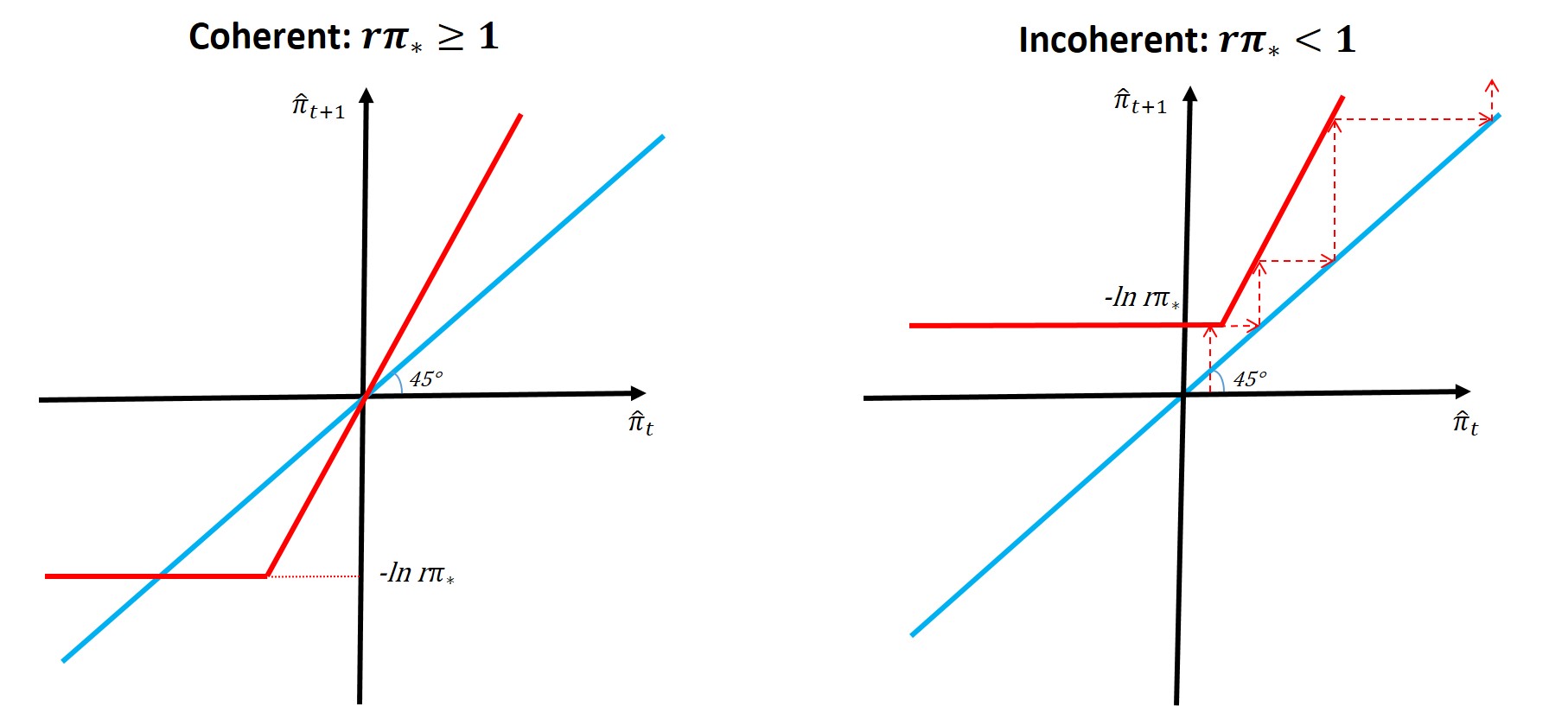
Figure 1: Illustration of coherency restriction $r\pi_{*}\geq 1$ under the absorbing state in Proposition 1. The red line plots $\hat{\pi}_{t+1}=\max\left\{-\log{r\pi_{*}},\psi\hat{\pi}_{t}\right\}$ with $\psi>1$ for two different values of $r\pi_{*}$. When $r\pi_{*}<1$, no bounded solution exists.

Proposition 1 focused only on the case $\psi>1$, but it is easy to see from the proof, as well as from the argument in Figure 1, that no support restrictions are needed when $\psi<1$: the model is always coherent when the Taylor rule is passive.

When the coherency condition in Proposition 1 holds, the stationary solutions of the transition equations represent fundamental solutions at which $\pi_{t}$ depends only on $M_{t}$ and not on its lags. Such solutions are also known as minimum state variable (MSV) solutions in the literature, because they involve the smallest number of state variables (in this case, only one). So, for this model, the same coherency condition that is required for existence of bounded fundamental solutions is also necessary and sufficient for the existence of MSV solutions, which is a subset of all fundamental solutions. This is noteworthy because many of the solution methods in the literature focus on MSV solutions, e.g., Fernández-Villaverde et al. (2015), Richter and Throckmorton (2015).

We conclude our analysis of this simple example by considering sunspot solutions. For simplicity, we assume there are no fundamental shocks, as in Mertens and Ravn (2014).

Proposition 2.

Suppose $M_{t}=r^{-1}$ with probability 1 and $\psi>1$, and let $\varsigma_{t}\in\{0,1\}$ be a first-order Markovian sunspot process that belongs to agents’ information set $\Omega_{t}$. Sunspot solutions to (3) exist if and only if $r^{-1}\leq\pi_{\ast}$.

Proposition 2 shows that the support restriction for the existence of sunspot solutions is exactly the same as for the existence of fundamental solutions (see the condition corresponding to the absorbing state in Proposition 1). Thus allowing for sunspot equilibria does not alter the essence of the coherency problem, as we further show in the next subsection.

2.2 Checking coherency of piecewise linear models

Many of the solution methods in the literature apply to (log)linear models, whose only nonlinearity arises from the lower bound constraint on interest rates, e.g., Eggertsson and Woodford (2003), Guerrieri and Iacoviello (2015), Kulish et al. (2017), Holden (2021). Let $Y_{t}$ be a $n\times 1$ vector of endogenous variables, $X_{t}$ be a $n_{x}\times 1$ vector of exogenous state variables, which could include a sunspot shock whose coefficients in the model are zero, $Y_{t+1|t}:=E\left(Y_{t+1}|\Omega_{t}\right)$, $X_{t+1|t}:=E\left(X_{t+1}|\Omega_{t}\right),$ and $s_{t}\in\left\{0,1\right\}$ an indicator variable that takes the value 1 when some inequality constraint is slack and zero otherwise. We consider models that can be written in the canonical form

$$A_{s_{t}}Y_{t}+B_{s_{t}}Y_{t+1|t}+C_{s_{t}}X_{t}+D_{s_{t}}X_{t+1|t}=0$$

(5)

where $A_{s},B_{s},C_{s},D_{s}$ are coefficient matrices, $a,b,c,d$ are coefficient vectors and $1_{A}$ is the indicator function that takes the value 1 if $A$ holds and zero otherwise.

Example ACS

Taking a log-linear approximation of (1) around $M_{t}=r^{-1}$ and $\pi_{t}=\pi_{\ast}$ we obtain $\hat{\pi}_{t+1|t}=\hat{R}_{t}+\hat{M}_{t+1|t},$ where $\hat{\pi}_{t}:=\log\left(\pi_{t}/\pi_{\ast}\right),$ $\hat{M}_{t}:=\log\left(rM_{t}\right),$ $\hat{R}_{t}:=\log R_{t}-\mu,$ $\mu:=\log\left(r\pi_{\ast}\right).$ Taking logs of (2) (no approximation) yields $\hat{R}_{t}=\max\left\{-\mu,\psi\hat{\pi}_{t}\right\}$ and combining the two equations yields $\hat{\pi}_{t+1|t}-\hat{M}_{t+1|t}-\max\left\{-\mu,\psi\hat{\pi}_{t}\right\}=0.$ The regime indicator is $s_{t}=1_{\left\{\psi\hat{\pi}_{t}+\mu>0\right\}}.$ This model can be put in the canonical form (5) with $Y_{t}=\hat{\pi}_{t},$ $X_{t}=\left(\hat{M}_{t},1\right)^{\prime},$ $A_{0}=0,$ $A_{1}=-\psi,$ $B_{0}=B_{1}=1,$ $C_{0}=\left(0,\mu\right),$ $C_{1}=\left(0,0\right),$ $D_{0}=D_{1}=\left(-1,0\right)$, $a=\psi,$ $b=0,$ $c=\left(0,\mu\right)^{\prime}$ and $d=\left(0,0\right)^{\prime}$. ∎

Example NK-TR

The basic three-equation New Keynesian model, consisting of a Phillips curve, an Euler equation and a Taylor rule, is

$$\hat{\pi}_{t} =\beta\hat{\pi}_{t+1|t}+\lambda\hat{x}_{t}+u_{t}$$ (6a)

$$\hat{x}_{t} =\hat{x}_{t+1|t}-\sigma\left(\hat{R}_{t}-\hat{\pi}_{t+1|t}\right)+\epsilon_{t}$$ (6b)

$$\hat{R}_{t} =\max\left\{-\mu,\psi\hat{\pi}_{t}+\psi_{x}\hat{x}_{t}+\nu_{t}\right\}$$ (6c)

where $\hat{\pi}_{t},\hat{R}_{t}$ were defined in the previous example and $\hat{x}_{t}$ is the output gap. It can be put in the canonical form (5) with $Y_{t}=\left(\hat{\pi}_{t},\hat{x}_{t}\right)^{\prime},$ $X_{t}=\left(u_{t},\epsilon_{t},\nu_{t},1\right)^{\prime}$, and coefficients given in A.2.1. ∎

Example NK-OP

The NK model with optimal discretionary policy replaces (6c) with

$$\gamma\hat{x}_{t}+\lambda\hat{\pi}_{t}=0,\quad\text{if}\quad\hat{R}_{t}>-\mu,\quad\text{or}\quad\gamma\hat{x}_{t}+\lambda\hat{\pi}_{t}<0,\quad\text{if}\quad\hat{R}_{t}=-\mu,$$ (7)

where $\gamma\geq 0$ is the weight the monetary authority attaches to output stabilization relative to inflation stabilization, see Armenter (2018), Nakata (2018) or Nakata and Schmidt (2019) for details. Substituting for $\hat{R}_{t}=-\mu$ in (6b) when the ZLB binds, the model can be written in terms of two equations: (6a) and $\hat{x}_{t}=(1-s_{t})\left[\hat{x}_{t+1|t}-\sigma\left(-\mu-\hat{\pi}_{t+1|t}\right)+\epsilon_{t}\right]-s_{t}\frac{\lambda}{\gamma}\hat{\pi}_{t}$, where $s_{t}=1_{\left\{\hat{\pi}_{t+1|t}+\frac{\hat{x}_{t+1|t}-\hat{x}_{t}+\epsilon_{t}}{\sigma}+\mu>0\right\}}$. This can be put in the canonical representation (5) with $Y_{t}=\left(\hat{\pi}_{t},\hat{x}_{t}\right)^{\prime}$, $X_{t}=\left(u_{t},\epsilon_{t},1\right)$, and coefficients given in A.2.1. ∎

A special case of (5) without expectations of the endogenous variables, i.e., $B_{0}=B_{1}=0$ and $b=0,$ is a piecewise linear simultaneous equations model with endogenous regime switching, whose coherency was analysed by GLM. We will now show how (5) with expectations can be cast into the model analysed by GLM when the shocks are Markovian with discrete support. This is a key insight of the paper.

Without much loss of generality, we assume that the state variables $X_{t}$ are first-order Markovian. We also focus on the existence of MSV solutions that can be represented as $Y_{t}=f\left(X_{t}\right)$ for some function $f\left(\cdot\right).$ Therefore, from now on, coherency of the model (5) is understood to mean existence of some function $f\left(\cdot\right)$ such that $Y_{t}=f\left(X_{t}\right)$ satisfies (5).

Assume that $X_{t}$ can be represented as a $k$-state stationary first-order Markov chain process with transition matrix $K$, and collect all the possible states $i=1,...,k$ of $X_{t}$ in a $n_{x}\times k$ matrix $\mathbf{X}$. Let $e_{i}$ denote the $i$th column of $I_{k}$, the identity matrix of dimension $k$, so that $\mathbf{X}e_{i}$ – the $i$th column of $\mathbf{X}$ – is the $i$th state of $X_{t}$. Note that the elements of the transition kernel are $K_{ij}=\Pr\left(X_{t+1}=\mathbf{X}e_{j}|X_{t}=\mathbf{X}e_{i}\right)$ and hence, $E\left(X_{t+1}|X_{t}=\mathbf{X}e_{i}\right)=\mathbf{X}K^{\prime}e_{i}.$ Let $\mathbf{Y}$ denote the $n\times k$ matrix whose $i$th column, $\mathbf{Y}e_{i}$, gives the value of $Y_{t}$ that corresponds to $X_{t}=\mathbf{X}e_{i}$ along a MSV solution. Therefore, along a MSV solution we have $E\left(Y_{t+1}|Y_{t}=\mathbf{Y}e_{i}\right)=E\left(Y_{t+1}|X_{t}=\mathbf{X}e_{i}\right)=\mathbf{Y}K^{\prime}e_{i}.$ Substituting into (5), $\mathbf{Y}$ must satisfy the following system of equations

$$0 =\left(A_{s_{i}}\mathbf{Y}+B_{s_{i}}\mathbf{Y}K^{\prime}+C_{s_{i}}\mathbf{X}+D_{s_{i}}\mathbf{X}K^{\prime}\right)e_{i}$$ (8)

$$s_{i} =1_{\left\{\left(a^{\prime}\mathbf{Y}+b^{\prime}\mathbf{Y}K^{\prime}+c^{\prime}\mathbf{X}+d^{\prime}\mathbf{X}K^{\prime}\right)e_{i}>0\right\}},\quad i=1,...,k.$$

This system of equations can be expressed in the form $F\left(\mathbf{Y}\right)=\kappa\left(\mathbf{X}\right)$, where $\kappa\left(\cdot\right)$ is some function of $\mathbf{X,}$ and $F\left(\cdot\right)$ is a piecewise linear continuous function of $\mathbf{Y}$. Specifically, let $J$ be a subset of $\left\{1,...,k\right\}.$ Then, we can write $F\left(\cdot\right)$ as

$$F\left(\mathbf{Y}\right)=\sum_{J}\mathcal{A}_{J}1_{\mathcal{C}_{J}}vec\left(\mathbf{Y}\right),$$ (9)

where $\mathcal{C}_{J}=\left\{\mathbf{Y}:\mathbf{Y\in\Re}^{n\times k},s_{i}=1_{\left\{i\in J\right\}}\right\}$ is defined by a particular configuration of regimes over the $k$ states given by $J$. If the piecewise linear function $F\left(\cdot\right)$ in (9) is invertible, then the system is coherent. This can be checked using Theorem 1 from GLM reproduced below.

Theorem (GLM).

Suppose that the mapping $F\left(\cdot\right)$ defined in (9) is continuous. A necessary and sufficient condition for $F\left(\cdot\right)$ to be invertible is that all the determinants $\det\mathcal{A}_{J},$ $J\subseteq\left\{1,...,k\right\}$ have the same sign.

The above determinant condition is straightforward to check. If the condition is satisfied, then the model has a unique MSV solution. If the condition fails, the model is not generically coherent, meaning that there will be values of $\mathbf{X}$ for which no MSV solution exists. Since $\mathbf{X}$ represents the support of the distribution of $X_{t}$, violation of the coherency condition in the (GLM). Theorem means that a MSV solution can only be found if we impose restrictions on the support of the distribution of the exogenous variables $X_{t}$.

Example ACS continued

Suppose $\hat{M}_{t}$ follows a two-state Markov Chain with transition kernel $K$, there are four possible subsets of $\left\{1,2\right\}$. Let PIR refer to a positive interest rate state when the ZLB constraint is slack and ZIR to a zero interest rate state when the ZLB constraint binds. Given $e_{1}:=(1,0)^{\prime}$, $e_{2}:=(0,1)^{\prime}$, the coefficients of (9) are

$$\mathcal{A}_{J_{1}}=A_{1}I_{2}+B_{1}K,$$ (PIR,PIR)

, (ZIR,PIR)

(PIR,ZIR)

(ZIR,ZIR)

(10)

where, as we showed previously, $A_{0}=0,$ $A_{1}=-\psi,$ and $B_{0}=B_{1}=1.$ From (10), we obtain $\det\mathcal{A}_{J_{1}}=\left(\psi-1\right)(1-p\allowbreak-q+\psi),$ $\det\mathcal{A}_{J_{2}}=p\left(1-\psi\right)+q-1,$ $\det\mathcal{A}_{J_{3}}=p-1+q\left(1-\psi\right),$ $\det\mathcal{A}_{J_{4}}\allowbreak=p+q-1.$ We focus on the case $\psi>1.$ Since $0\leq p,q\leq 1,$ it follows immediately that $\det\mathcal{A}_{J_{1}}$ is positive while $\det\mathcal{A}_{J_{2}}$ and $\det\mathcal{A}_{J_{3}}$ are both negative, so the coherency condition in the (GLM). Theorem is violated. ∎

The next proposition states that the conclusion that an active Taylor rule leads to a model that is not generically coherent generalizes to the basic three-equation NK model. The following one states that the same conclusion applies to a NK model with optimal policy.

Proposition 3.

The NK-TR model given by equations (6a) with $u_{t}=0$, (6b) with $\epsilon_{t}$ following a two-state Markov chain process, and the active Taylor rule (6c) with $\psi>1$ and $\psi_{x}=\nu_{t}=0$, is not generically coherent.

Proposition 4.

The NK-OP model given by equations (6a) with $u_{t}=0$, (6b) with $\epsilon_{t}$ following a two-state Markov chain process, and the optimal discretionary policy (7) is not generically coherent.

Proposition 4 proves that there are values of the shocks for which no MSV equilibrium exists, thus formally corroborating the numerical findings in Armenter (2018) about non-existence of Markov-perfect equilibria (which we call MSV solutions) in the NK-OP model.

Analogously to Proposition 1 in the previous subsection, we can characterize the support restrictions for existence of a solution in the special case given by Assumption 1, such that $p<1$ (transitory state) and $q=1$ (absorbing state), with support of $\hat{M}_{t}$ equal to $(-r^{L})$ and $0$, respectively.

Proposition 5.

Consider the NK-TR model of Proposition 3. Suppose further that $\epsilon_{t}=-\sigma\hat{M}_{t+1|t}$, where $M_{t}$ satisfies Assumption 1, and define $\theta:=\frac{\left(1-p\right)\left(1-p\beta\right)}{p\sigma\lambda}$. A MSV solution exists if and only if

either $$\theta>1\text{ and }r^{-1}\leq\pi_{\ast},$$ (11a)

or $$\theta\leq 1,\text{ }r^{-1}\leq\pi_{\ast}\text{ and }-r^{L}\leq\log(r\pi_{*})\left(\frac{\psi-p}{\psi p}+\frac{\theta}{\psi}\right).$$ (11b)

Figure 2 helps to grasp the economic intuition. The $AD$ curve is piecewise linear depending on whether the economy is at the ZLB ($AD^{ZLB}$) or monetary policy follows the Taylor rule ($AD^{TR}$). The negative shock shifts the $AD$ curve to the left. In the transitory state, there are four possibilities depending on the value of $\theta$, and on the equilibrium in the absorbing state, which can be either a PIR one or a ZIR one (see Appendix A.2.4).

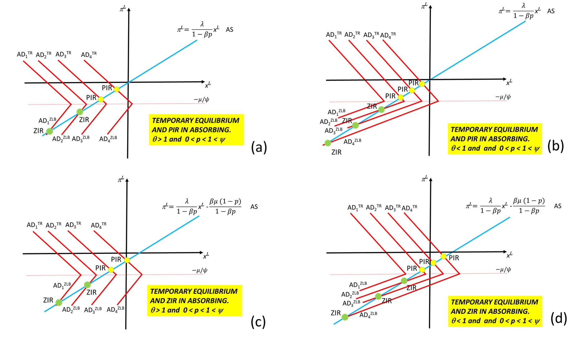
Figure 2: The temporary state in the NK model when $\psi>1$.

When $\theta>1$, the $AS$ is flatter than $AD^{ZLB}$, and the $AS-AD$ system is described by the curves plotted in the left column of Figure 2 for the two cases when the absorbing state is PIR on the top, i.e., panel (a), and when the absorbing state is ZIR on the bottom, i.e., panel (c). Inspection of these two graphs shows there is always a solution in both cases. Hence, when $\theta>1,$ the only necessary support restriction is $\left(r\pi_{\ast}\right)^{-1}\leq 1$, which guarantees the existence of an equilibrium in the absorbing state, as stated in (11a). Next, turn to the case $\theta\leq 1.$ The $AS$ is steeper than $AD^{ZLB},$ and the $AS-AD$ system is described by the curves plotted in the right column of Figure 2 for the two cases when the absorbing state is PIR on the top, i.e., panel (b), and when the absorbing state is ZIR on the bottom, i.e., panel (d). Clealry, a further support restriction is needed on the value of the shock in the transitory state to avoid the $AD$ curve being completely above the $AS$ curve. Intuitively, the negative shock cannot be too large (in absolute value) for an equilibrium (actually two equilibria in this case) to exist. This is what the second condition (11b) guarantees.

Proposition 6.

Consider the NK-OP models of Proposition 4. Suppose further that $\epsilon_{t}=-\sigma\hat{M}_{t+1|t}$, where $M_{t}$ satisfies Assumption 1, and define $\theta:=\frac{\left(1-p\right)\left(1-p\beta\right)}{p\sigma\lambda}$. A MSV solution exists if and only if

either $$\theta>1\text{ and }r^{-1}\leq\pi_{\ast},$$ (12a)

or $$\theta\leq 1,\text{ }r^{-1}\leq\pi_{\ast}\text{ and }-r^{L}\leq\frac{\log(r\pi_{*})}{p}.$$ (12b)

Figure 3 helps to grasp the economic intuition. The $AD$ curve is piecewise linear depending on whether the economy is at the ZLB ($AD^{ZLB}$) or monetary policy follows the optimal rule ($AD^{OP}$). The negative shock shifts the $AD^{ZLB}$ curve upward. In the transitory state, there are four possibilities. When $\theta>1$, the $AS$ is flatter than $AD^{ZLB}$ and the relevant plots are panel (a) and (c) on the left column, depending whether agents expect the absorbing state to be a PIR or a ZIR. There is always a solution in both cases, so again we conclude that when $\theta>1,$ the only necessary support restriction is $\left(r\pi_{\ast}\right)^{-1}\leq 1$, as stated in (12a). Instead, when $\theta\leq 1$, the $AS$ is steeper than $AD^{ZLB},$ and the relevant plots are the one on the right column. There exists an equilibrium (actually two equilibria) if and only if $(-r^{L})$ is below a threshold level, which is given by $\frac{\mu}{p},$ as stated by (12b) (see Appendix A.2.5).

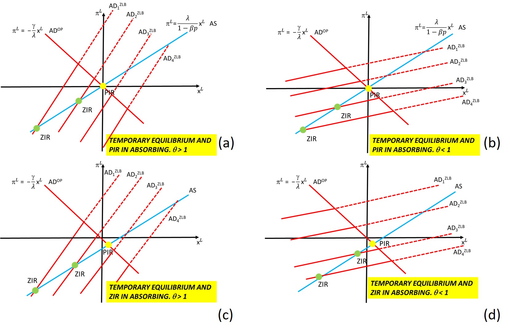
Figure 3: The temporary state in the NK-OP model.

The literature on confidence-driven equilibria (e.g., Mertens and Ravn, 2014) emphasised the possibility of sunspots when $\theta\leq 1$. Propositions 5 and 6 do not consider sunspot equilibria. Existence of sunspot equilibria can be examined by including a sunspot shock in the exogenous state variables $X_{t}$. For example, analogously to Proposition 2, it can be shown that if the discount factor shock $M_{t}$ takes a single value $1/r$ and we allow for a binary sunspot process $\varsigma_{t}$ with transition matrix $K_{\varsigma}$, the NK-TR model with $\psi>1$ is not generically coherent, and an equilibrium exists if and only if $r^{-1}\leq\pi_{*}$.

In the case of the NK-OP model, Nakata (2018) and Nakata and Schmidt (2019) consider only the case when the ZLB always binds in the ‘low’ state, corresponding to $-pr^{L}>\log(r\pi_{*})$. Because this excludes (12b), the condition for existence of a Markov-perfect (MSV) equilibrium given in Nakata and Schmidt (2019, Prop. 1) corresponds to (12a), which they express as a restriction on the transition probabilities, equivalent to $\theta>1$ in (12a), see Appendix A.2.7 for details. Therefore, Proposition 6 corroborates and extends the existence results in Nakata and Schmidt (2019) by highlighting that existence requires restrictions on the values the shocks can take (support) rather than on the transition probabilities.

Finally, note that as $\sigma$ gets large, $\theta$ goes to zero and condition (11) reduces to

$$r^{-1}\leq\pi_{\ast},\quad\text{and\quad}-r^{L}\leq\log\left(r\pi_{\ast}\right)\frac{\psi-p}{\psi p},$$ (13)

which is the support restriction for Example ACS.

2.3 More about the nature of the support restrictions

To shed some further light on the nature of the support restrictions, we consider a modification of Example ACS that allows us to characterize the support restrictions analytically even when there are multiple shocks and the distribution of the shocks is continuous. Specifically, we replace the contemporaneous Taylor rule (2) with a purely forward-looking one that also includes a monetary policy shock $\nu_{t}$. In log-deviations from steady state, the forward-looking Taylor rule is $\hat{R}_{t}=\max(-\mu,\psi\hat{\pi}_{t+1|t}+\nu_{t})$. Substituting for $\hat{\pi}_{t+1|t}=\hat{R}_{t}+\hat{M}_{t+1|t}$ from the log-linear Fisher equation, we obtain the univariate equation

$$\hat{R}_{t}=\max\left\{-\mu,\psi\hat{R}_{t}+\psi\hat{M}_{t+1|t}+\nu_{t}\right\}.$$ (14)

The advantage of a forward-looking Taylor rule in this very simple model is that it allows us to substitute out the expectations of the endogenous variable $\hat{\pi}_{t+1|t}$, and therefore obtain an equation that is immediately piecewise linear in the remaining endogenous variable $\hat{R}_{t}$. Application of the (GLM). Theorem then shows that the model is not generically coherent when $\psi>1$. This is shown graphically in Figure 4, where the left-hand side (LHS) and right-hand side (RHS) of (14) are shown in blue and red, respectively. When $\psi>1$, (14) may have no solution, an example of which is shown on the left graph in Figure 4; or it may have two solutions, which is shown in the graph on the right in Figure 4. The latter graph also highlights the range of values of the shocks corresponding to incoherency – when the positively sloped part of the red curve lies in the grey area, and the ones for which two solutions exist – when the positively sloped part of the red curve lies to the right of the grey area. The support restrictions required for existence of a solution are $\psi\hat{M}_{t+1|t}+\nu_{t}\leq(\psi-1)\mu$.

Figure 4: Illustration of the restriction on the support of $\hat{M}_{t+1|t},\nu_{t}$ in the model given by the intersection between the LHS of (14), blue line, and the RHS of (14), red line.

Suppose further that $\hat{M}_{t}$ follows the AR(1) process $\hat{M}_{t}=\rho\hat{M}_{t-1}+\sigma\epsilon_{t}$ with $E_{t-1}\epsilon_{t}=0$, which is the continuous counterpart to the Markov Chain representation we used previously. The support restrictions can then be equivalently rewritten as

$$\nu_{t}\leq-\psi\rho\sigma\epsilon_{t}-\psi\rho^{2}\hat{M}_{t-1}-\left(1-\psi\right)\log\left(r\pi_{\ast}\right),\text{ when }\psi>1.$$ (15)

Condition (15) has important implications that have been overlooked in the literature on estimation of DSGE models with a ZLB constraint: the shocks $\epsilon_{t}$ and $\nu_{t}$ cannot be independently distributed over time, nor can they be independent of each other.

First, suppose $\nu_{t}=0$, so the only shock driving the model is $\epsilon_{t}$. Condition (15) says that $\epsilon_{t}$ cannot be independently and identically distributed over time, since the support of its distribution depends on past $\hat{M}_{t}$, and hence, past $\epsilon_{t}$. The presence of state variables ($\hat{M}_{t}$) will generally cause support restrictions to depend on the past values of the state variables.

Second, condition (15) states that the monetary policy shock cannot be independent of the real shock since the support of their distribution cannot be rectangular. Specifically, the monetary policy shock cannot be too big relative to current and past shocks to the discount factor if we are to rule out incoherency.

If these shocks are structural shocks in a DSGE model, such necessary support restrictions are difficult to justify. Structural shocks are generally assumed to be orthogonal. In our opinion, it is hard to make sense of structural shocks whose supports depend on the value of the other shocks in a time-dependent way, as well as on the past values of the state variables. We believe this is a substantive problem for any DSGE model with a ZLB constraint, and, possibly, more generally, with any kinked constraint.

A possible solution to this problem is to interpret condition (15) as a constraint on the monetary policy shock $\nu_{t}$. When a very adverse shock hits the economy, monetary policy has to step in to guarantee the existence of an equilibrium, that is, to avoid the collapse of the economy. In a sense, this can represent what we witnessed after the Great Financial Crisis or after the COVID-19 pandemic: central banks engaged in massive operations through unconventional monetary policy measures (beyond the standard interest rate policy) in response to these large negative shocks. Hence, $\nu_{t}$ could represent what is currently missing in the simple Taylor rule or in the optimal policy problem to describe what monetary policy needs to do to guarantee the existence of an equilibrium facing very negative shocks and a ZLB constraint. This positive interpretation of condition (15) calls for going beyond these descriptions of monetary policy behavior to model explicitly monetary policy conduct such that incoherency disappears. An alternative way, presented in Subsection 2.5 below, relates to the use of unconventional monetary policy modelled via a shadow rate.

2.4 The Taylor coefficient and the coherency and completeness conditions

In the examples above, we saw that active Taylor rules ($\psi>1$) lead to incoherency, so restrictions on the support of the shocks are required for equilibria to exist. More generally, we can use the (GLM). Theorem to find the range of parameters of the models that guarantee coherency without support restrictions. In this subsection, we investigate this question in piecewise linear models with discrete shocks that follow a generic $k$-state Markov Chain.

The main result of this subsection is that the Taylor rule needs to be passive for the coherency and completeness condition in the (GLM). Theorem to be satisfied in the NK model. More generally, there is an upper bound, $\bar{\psi}_{k}$, on the Taylor rule coefficient $\psi$, which depends on parameters and on the number of states $k$, and it is always less than one.

We start with an analytical result for the special case with two states $k=2$.

Proposition 7.

Consider the NK model given by (6) with $\psi_{x}=u_{t}=\nu_{t}=0$ and suppose $\epsilon_{t}$ follows a Markov Chain with two states $\epsilon^{1},\epsilon^{2}$ and transition probabilities $p=\Pr(\epsilon_{t+1}=\epsilon^{1}\allowbreak|\epsilon_{t}=\epsilon^{1})$ and $q=\Pr(\epsilon_{t+1}=\epsilon^{2}\allowbreak|\epsilon_{t}=\epsilon^{2})$ and define

$$\psi_{p,q,\beta,\sigma\lambda}:=p+q-1-\frac{\left(2-p-q\right)\left(1-p\beta-q\beta+\beta\right)}{\sigma\lambda}.$$ (16)

The coherency condition in the (GLM). Theorem holds if and only if

either $$\psi_{p,q,\beta,\sigma\lambda}<0\text{ and }\psi_{p,q,\beta,\sigma\lambda}<\psi<1,$$ (17a)

or $$\psi_{p,q,\beta,\sigma\lambda}>0\text{ and }\psi<\psi_{p,q,\beta,\sigma\lambda}\leq 1.$$ (17b)

Again, the coherency condition depends on the slopes of the AS (6a) and AD (6b) curves. However, in all cases, it rules out $\psi>1$, generalizing Proposition 3. If one of the states is absorbing, $q=1$, then $\psi_{p,q,\beta,\sigma\lambda}=p-\frac{\left(1-p\right)\left(1-p\beta\right)}{\sigma\lambda},$ and the condition in (17a) $\psi_{p,q,\beta,\sigma\lambda}<0$ is equivalent to $\theta>1$, as in (11a) in Proposition 5, implying that the slope of the AS curve is flatter than the one of the AD curve under ZLB in the temporary state.

Another important special case is $p=q=(1+\rho)/2$, where $\rho\in(-1,1)$ is the autocorrelation coefficient of the shock $\epsilon_{t}$. In that case, we obtain $\psi_{p,q,\beta,\sigma\lambda}=\rho-\frac{\left(1-\rho\right)\left(1-\rho\beta\right)}{\sigma\lambda}$. This can be thought of as a two-state approximation of a continuous AR(1) process for $\epsilon_{t}$. We can evaluate the coherency condition numerically for a $k$-state Rouwenhorst (1995) approximation of an AR(1) process with $k>2$. Table 1 reports the coherency condition for various calibrations of the model found in Mertens and Ravn (2014), Eggertsson and Singh (2019) and Bilbiie (2018). For example, when $\rho\sigma\lambda<\left(1-\rho\right)\left(1-\rho\beta\right)$, we verified numerically to 6 decimal digit precision that the coherency condition remains $\psi<1$, that is, (17a) holds for all $k\leq 30$. In the opposite case, the coherency condition is (17b), and $\bar{\psi}_{k}$ can get considerably smaller for large values of $\rho$ and $\sigma\lambda$. For any given values of $\rho$ and $\sigma\lambda$, $\bar{\psi}_{k}$ seems to converge to some value that is bounded away from zero (see the last column of Table 1). As discussed previously, Example ACS is a special case that obtains when $\sigma$ is large. In that case, $\bar{\psi}_{k}$ tends to zero with $k$, which suggests that the coherency condition is not satisfied for any $\psi>0$ in the ACS model with a continuously distributed AR(1) shock.

Table 1: Coherency condition $\psi<\bar{\psi}$ for different calibrations of the NK model

Paper	$\beta$	$\sigma$	$\lambda$	$\mu$	$\rho$	$\bar{\psi}$
MR2014 FD	0.99	1	0.4479	0.01	0.4	1
MR2014 CD	0.99	1	0.4479	0.01	0.7	0.494
Bilbiie (2018)	0.99	1	0.02	0.01	0.8	1
	0.99	1	0.2	0.01	0.8	0.592
ES2019 GD	0.9969	0.6868	0.0091	0.0031	0.9035	1
ES2019 GR	0.997	0.6202	0.0079	0.003	0.86	1

Notes: MR2014: Mertens and Ravn (2014), FD: Fundamental-driven, CD: Confidence-driven; ES2019: Eggertsson and Singh (2019), GD: Great Depression, GR: Great Recession. These papers assume an absorbing state and $\rho$ corresponds to the persistence probability of the transitory state.

2.5 Coherency with unconventional monetary policy

In this subsection we show that UMP can relax the restrictions for coherency in the NK model. An UMP channel can be added to the model in Example NK-TR using a ‘shadow rate’ $\hat{R}_{t}^{\ast}$ that represents the desired UMP stance when it is below the ZLB.

Consider a model of bond market segmentation (Chen et al., 2012), where a fraction of households can only invest in long-term bonds. In such a model, the amount of long-term assets held by the private sector affects the term premium and provides an UMP channel via long-term asset purchases by the central bank. If we assume that asset purchases (quantitative easing) follow a similar policy rule to the Taylor rule, i.e., react to inflation deviation from target, then the IS curve (6b) can be written as (see Appendix A.4)

$$\hat{x}_{t} = \hat{x}_{t+1|t}-\sigma\left((1-\xi)\hat{R}_{t}+\xi\hat{R}_{t}^{\ast}-\hat{\pi}_{t+1|t}\right)+\epsilon_{t},$$ (18)

$$\hat{R}_{t} = \max\left\{-\mu,\hat{R}_{t}^{\ast}\right\},\quad\hat{R}_{t}^{*}=\psi\hat{\pi}_{t}+\psi_{x}\hat{x}_{t}+\nu_{t},$$ (19)

where $\xi$ is a function of the fraction of households constrained to invest in long-term bonds, the elasticity of the term premium with respect to the stock of long term bonds and the intensity of UMP. The standard NK model (6) arises as a special case with $\xi=0$.

The conditions for coherency can be derived analytically in the case of a single AD shock with a two-state support, analogously to Proposition 7.

Proposition 8.

Consider the NK model given by (6a), (18) and (19) with $\psi_{x}=u_{t}=\nu_{t}=0$ and suppose $\epsilon_{t}$ follows a Markov Chain with one absorbing state and one transitory state that persists with probability $p$. Then, the coherency condition in the (GLM). Theorem holds if and only if

$$\psi>\max\left(1,\frac{1}{\xi}\right),$$ (20a)

or $$\max\left(\psi_{p,1,\beta,\sigma\lambda},\frac{\psi_{p,1,\beta,\sigma\lambda}}{\xi}\right)<\psi<\min\left(1,\frac{1}{\xi}\right),$$ (20b)

$$\text{or}\quad\psi <\min\left(\psi_{p,1,\beta,\sigma\lambda},\frac{\psi_{p,1,\beta,\sigma\lambda}}{\xi}\right),$$ (20c)

where $\psi_{p,1,\beta,\sigma\lambda}\leq 1$ is defined in (16).

As $\xi$ goes to zero, the model reduces to the standard NK model (6), and the coherency condition (20) reduces to (17). We already established that in that case there are no values of $\psi>1$ that lead to coherency, i.e., an active Taylor rule violates the coherency condition. However, when UMP is present and effective, i.e., $\xi>0$, condition (20a) shows that an active Taylor rule can still lead to coherency, i.e., a MSV solution exists without support restrictions. For example, the value $\psi=1.5$ for the Taylor rule coefficient used in typical calibrations leads to coherency if $\xi>2/3$. This is consistent with the estimation results reported in Ikeda et al. (2020), who find the identified set of $\xi$ to be $\left[0.74,0.76\right]$ using postwar U.S. data.

2.6 Endogenous state variables

Up to this point, we analysed models without endogenous dynamics. In this subsection, we describe the challenges posed by endogenous dynamics and discuss various solutions.

We can add endogenous dynamics to the canonical model (5) as follows:

$$A_{s_{t}}Y_{t}+B_{s_{t}}Y_{t+1|t}+C_{s_{t}}X_{t}+D_{s_{t}}X_{t+1|t}+H_{s_{t}}Y_{t-1}=0$$

(21)

where $Y_{t}$ is a $n\times 1$ vector of (nonpredetermined) endogenous variables, $X_{t}$ is a $n_{x}\times 1$ vector of exogenous state variables, $H_{s}$ are $n\times n$ coefficient matrices, $h$ is an $n\times 1$ coefficient vector, and the remaining coefficients were already defined above in (5).

Example NK-ITR

(NK model with Inertial Taylor rule) A generalization of the basic three-equation NK model in Example NK-TR is obtained by replacing (6c) with $\hat{R}_{t}=\max\{-\mu,\allowbreak\phi\hat{R}_{t-1}+\psi\hat{\pi}_{t}+\psi_{x}\hat{x}_{t}+\nu_{t}\}$. It can be put in the canonical form (21) with $Y_{t}=\left(\hat{\pi}_{t},\hat{x}_{t},\hat{R}_{t}\right)^{\prime},$ $X_{t}=\left(u_{t},\epsilon_{t},\nu_{t},1\right)^{\prime}$, and coefficient matrices given in Appendix A.5.1. ∎

As before, we study the existence of MSV solutions, which are of the form $Y_{t}=f\left(Y_{t-1},X_{t}\right)$. We also assume as before that $X_{t}$ follows a $k$-state Markov chain with transition kernel $K$ and support $\mathbf{X\in\Re}^{n_{x}\times k}$, so that the $i$th column of $\mathbf{X,}$ i.e., $\mathbf{X}e_{i},$ gives the value of $X_{t}$ in state $i=1,\ldots,k$. In models without endogenous state variables (5), we can represent the MSV solution $Y_{t}=f\left(X_{t}\right)$ exactly by a constant $n\times k$ matrix $\mathbf{Y}$, since $Y_{t}$ has exactly $k$ points of support corresponding to the $k$ states of $X_{t}$ that are constant over time. However, with endogenous states the support of $Y_{t}$ will vary endogenously over time along a MSV solution $Y_{t}=f\left(Y_{t-1},X_{t}\right)$ through the evolution of $Y_{t-1}$, and thus, it cannot be characterized by a constant matrix $\mathbf{Y}$. That is, the matrix of support points of $Y_{t}$ – which we previously defined by the time-invariant matrix $\mathbf{Y}$ because the support of $X_{t}$ is time-invariant – must now be a function of $Y_{t-1}$, too. Hence while without endogenous state variables along a MSV solution we have $E\left(Y_{t+1}|Y_{t}=\mathbf{Y}e_{i}\right)=E\left(Y_{t+1}|X_{t}=\mathbf{X}e_{i}\right)=\mathbf{Y}K^{\prime}e_{i}$, when there are endogenous state variables we have $E(Y_{t+1}|Y_{t}\allowbreak=\mathbf{Y}_{t}e_{i},X_{t}\allowbreak=\mathbf{X}e_{i})\allowbreak=\mathbf{Y}_{t+1}^{i}K^{\prime}e_{i},$ where $\mathbf{Y}_{t+1}^{i}$ gives the support of $Y_{t+1}$ when $Y_{t}$ is in the $i$th state. The problem is that the support of $Y_{t}$ is rising exponentially for any given initial condition $Y_{0},$ so the MSV solution cannot be represented by any finite-dimensional system of piecewise linear equations. This makes the analysis of Subsection 2.2 generally inapplicable.

To make progress, we will consider solving the model backwards from some terminal condition in a way that nests the case of no endogenous dynamics that we studied earlier. We will assume, for simplicity of notation, that the endogenous state variable is a scalar, i.e., $H_{s_{t}}Y_{t-1}=h_{s_{t}}y_{t-1}$ in (21), where $h_{s_{t}}$ is $n\times 1$ and $y_{t}:=g^{\prime}Y_{t}$ is a linear combination of $Y_{t}$, for some known $n\times 1$ vector $g$, as in Example NK-ITR, where $g=\left(0,0,1\right)^{\prime}$. Next, suppose there is a date $T$ such that for all $t\geq T$, the MSV solution $f\left(y_{t-1},X_{t}\right)$ can be represented in the form $\mathbf{Y}_{t}=\mathbf{G}y_{t-1}+\mathbf{Z}$, with $n\times k$ matrices $\mathbf{G}$ and $\mathbf{Z}$. This is a matrix representation of a general possibly nonlinear function $f(y_{t-1},X_{t})$. The matrix $\mathbf{Z}$ represents the part of $Y_{t}$ that depends only on the exogenous variables $X_{t}$. When there are no endogenous states, we have $\mathbf{G}=0$, so $\mathbf{Y}_{t}=\mathbf{Z}$, which we denoted by $\mathbf{Y}$ in (8) above. Each column of $\mathbf{G}$ gives the coefficients on $y_{t-1}$ in the MSV solution that correspond to each different state of $X_{t}$. For example, if $k=2$, then the endogenous dynamics in the low state $i=1$, say, can be different from the high state $i=2$. If $i=1$ were a ZIR and $i=2$ were a PIR, the endogenous dynamics could differ across regimes, as shown analytically in the example below.

In the case of no endogenous dynamics, we analysed the solution of $\mathbf{Y}(=\mathbf{Z}$ here) using the method of undetermined coefficients, see equation (8) above. The corresponding equation for the model with endogenous dynamics is

$$0 =\left(A_{s_{t,i}}\mathbf{G}e_{i}+h_{s_{t,i}}+B_{s_{t,i}}\mathbf{G}K^{\prime}e_{i}g^{\prime}\mathbf{G}e_{i}\right)y_{t-1}$$ (22)

$$+\left(A_{s_{t,i}}\mathbf{Z}+B_{s_{t,i}}\mathbf{G}K^{\prime}e_{i}g^{\prime}\mathbf{Z}+B_{s_{t,i}}\mathbf{Z}K^{\prime}+C_{s_{t,i}}\mathbf{X}+D_{s_{t,i}}\mathbf{X}K^{\prime}\right)e_{i},$$

for all $i=1,\ldots,k$, see A.5.2. Note that (22) exactly nests (8) when $h_{s_{t,i}}=0$, $G=0$ and $\mathbf{Z}=\mathbf{Y}$. Given a particular regime configuration $J\subseteq\left\{1,\ldots,k\right\}$, which determines in which of the states the constraint is slack, $s_{t,i}=1$, (22) gives a system of $2nk$ polynomial equations in the $2nk$ unknowns $\mathbf{G}$ and $\mathbf{Z}$ by equating the coefficients on $y_{t-1}$ and the constant terms to zero, respectively. Unfortunately, because this system of equations is not piecewise linear in $\mathbf{G}$ and $\mathbf{Z}$, we cannot use the (GLM). Theorem to check coherency. Therefore, one would need to resort to a brute force method of going through all possible $2^{k}$ regime configurations $J$ and checking if there are any solutions that satisfy the inequality constraints. Since $y_{t-1}$ is endogenous, one would need to solve the system backwards subject to some initial condition $y_{0}$, and then check coherency for all possible values of $y_{0}$. An algorithm for doing this is given in Appendix A.5.2 .

Example NK-ITR continued

Again, it is possible to obtain some analytical results in the special case of the model in Example NK-ITR if we assume, as in Proposition 5, that $\psi_{x}=u_{t}=\nu_{t}=0$ and that $\epsilon_{t}=-\sigma\hat{M}_{t+1|t}$, where $M_{t}$ satisfies Assumption 1. Here, we report results on the existence of a MSV solution such that the economy is in a ZIR in the temporary state where $\hat{M}_{t}=-r^{L}$ and then converges to a PIR in the absorbing state where $\hat{M}_{t}=0$. In other words, we report the support restrictions needed for a ZIR to exist in the temporary state, given that the agents expect to move to the stable manifold of the PIR system as soon as the shock vanishes. Appendix A.5.3 shows that such a solution exists if and only if

either $$\theta>1\text{ and }r^{-1}\leq\pi_{\ast}\text{ and }-r^{L}\geq-\bar{r}^{L},$$ (23a)

or $$\theta\leq 1,\text{ }r^{-1}\leq\pi_{\ast}\text{ and }-r^{L}\leq-\bar{r}^{L},$$ (23b)

where

$$-\bar{r}^{L}=\mu\left(\frac{\psi-p}{\psi p}+\frac{\theta}{\psi}+\frac{\phi}{\psi}\left(1-\theta\right)-(1-p)\frac{\lambda\gamma_{x}+\gamma_{\pi}\left[\beta(1-p)+\lambda\sigma\right]}{\lambda\sigma p}\right),$$ (24)

$\theta:=\frac{\left(1-p\right)\left(1-p\beta\right)}{p\sigma\lambda}$ and $\gamma_{x},\gamma_{\pi}$ are functions of the model’s parameters. $\gamma_{x},\gamma_{\pi}$ define the slope of the stable manifold of the PIR system such that in the absorbing state $\hat{\pi}_{t}$ and $\hat{x}_{t}$ will travel to the PIR steady state along the paths $\hat{\pi}_{t}=\gamma_{\pi}\hat{R}_{t-1}$ and $\hat{x}_{t}=\gamma_{x}\hat{R}_{t-1}$. This result nests the corresponding analysis in Proposition 5, because if $\phi=0$ then $\gamma_{\pi}=\gamma_{x}=0$ and (23b) collapses to (11b), where $-r^{L}\leq\log(r\pi_{\ast})\allowbreak\left(\frac{\psi-p}{\psi p}+\frac{\theta}{\psi}\right)$. (23) shows that, for a ZIR-PIR to exist, the negative shock should be large enough in absolute value when $\theta>1$, while it should be small enough in absolute value when $\theta\leq 1.$ Numerical results (not reported) show that, if that condition is not satisfied, then there is a PIR-PIR solution if $\theta>1$, and there is no solution if $\theta\leq 1$, as implied by Proposition 5 for the case of no inertia.

The effects of inertia on the support restrictions needed for the existence of an equilibrium when $\theta\leq 1$ can be evaluated numerically, since we do not have analytic expressions for $\gamma_{\pi}$ and $\gamma_{x}$. Figure 5 shows the lower bound $\bar{r}^{L}$ as a function of $\phi$ for the two calibrations given in Table 1 where $\theta\leq 1$. Given that the shock needs to be above the lower bound (i.e., smaller in absolute value) for the equilibrium to exists, the graph reveals that inertia relax the support restrictions.

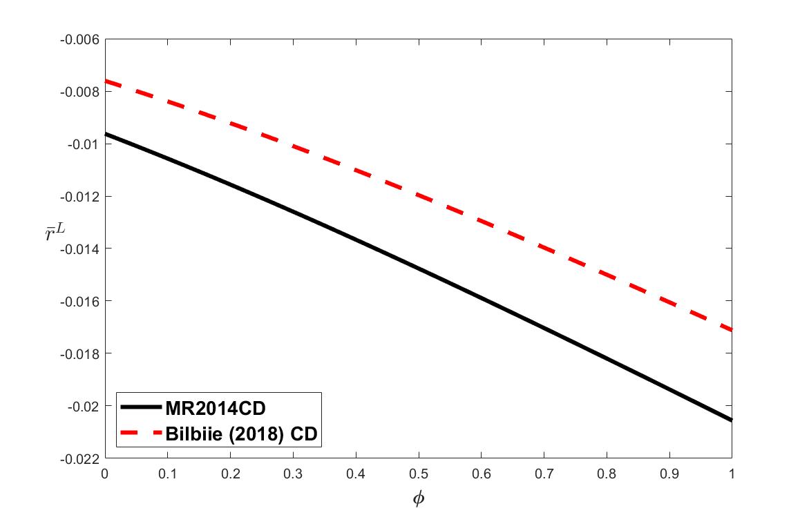
Figure 5: $\bar{r}^{L}$ as a function of $\phi$, using parameters from Mertens and Ravn (2014) and Bilbiie (2018) calibrations shown in Table 1 where $\theta<1$.

2.6.1 Quasi differencing

In a very special case, we can analyse the coherency of the model using the (GLM). Theorem.

Assumption 2.

Assume the first $n_{1}$ elements $Y_{1t}$ of $Y_{t}=\left(Y_{1t}^{\prime},Y_{2t}^{\prime}\right)^{\prime}$ in model (5) are predetermined, $B_{0},B_{1}$ are invertible, and there exists a $n\times n$ invertible matrix $Q$ such that $Q^{-1}B_{s}^{-1}A_{s}Q=\Lambda_{s}$ is upper triangular for both $s=0,1.$ Let $Q_{1}$ denote the first $n_{1}$ elements of $Q,$ and assume also that $a^{\prime}Q_{1}=b^{\prime}Q_{1}=0.$

The first part of Assumption 2 is satisfied for commuting pairs of matrices, but commutation is not necessary. This assumption is clearly restrictive, but not empty, see Example ACS-STR below.

If Assumption 2 holds, then we can remove the predetermined variables $Y_{1t}$ from (5) by premultiplying the equation by some $n_{2}\times n$ matrix $(-\Gamma,I_{n_{2}})$, where $\Gamma$ is $n_{2}\times n_{1}$ (see Appendix A.5.4). Intuitively, we transform the original system to one that does not involve any predetermined variables by taking a ‘quasi difference’ of $Y_{2t}$ from the predetermined variables $Y_{1t},$ say $\widetilde{Y}_{t}:=Y_{2t}-\Gamma Y_{1t}$. This is typically possible in linear models, but it is not, in general, possible in piecewise linear models because the ‘quasi difference’ coefficient $\Gamma$ needs to be the same across all regimes. Assumption 2 ensures this is possible. Since the model in $\widetilde{Y}_{t}$ does not have any predetermined variables and is still of the form (5), we can analyze its coherency using the (GLM). Theorem as in Subsection 2.2.

Example ACS-STR

Consider a generalization of Example ACS where the Taylor rule $\hat{R}_{t}=\max\left\{-\mu,\psi\hat{\pi}_{t}\right\}$ is replaced with $\hat{R}_{t}=\max\left\{-\mu,\phi\hat{R}_{t-1}+\psi\hat{\pi}_{t}\right\}$. Appendix A.5.5 shows that this model satisfies Assumption 2, applies the (GLM). Theorem and analyzes the solutions. When the exogenous shock satisfies Assumption 1, the coherency condition is $\psi<p-\phi$, which generalizes the one found earlier without inertia: $\psi<p$. When $\psi>1$, the requisite support restriction on $r^{L}$ is $-r^{L}<\mu\frac{\psi+\phi-p}{p\psi}$. For $\phi>0$, this support restriction is weaker than the one for the noninertial model given in (13). ∎

3 The incompleteness problem

This Section explores the multiplicity of the MSV solutions in piecewise linear models of the form (5). The main message is that when the CC condition of the (GLM). Theorem is not satisfied, but the support of the distribution of the shocks is restricted appropriately, there are many more MSV solutions than are typically considered in the literature. This is distinct from the usual issue of indeterminacy in models without occasionally binding constraints.

As we discussed in Subsection 2.2, when the state variables $X_{t}$ follow a $k$-state Markov chain, these models can be written as $F\left(\mathbf{Y}\right)=\kappa\left(\mathbf{X}\right)$, where $F(\cdot)$ is the piecewise linear function (9), and all possible solutions correspond to $\mathbf{Y=}\mathcal{A}_{J}^{-1}\kappa\left(\mathbf{X}\right)$ for each $J\subseteq\left\{1,\ldots,k\right\}$. Thus, there are up to $2^{k}$ possible MSV solutions.

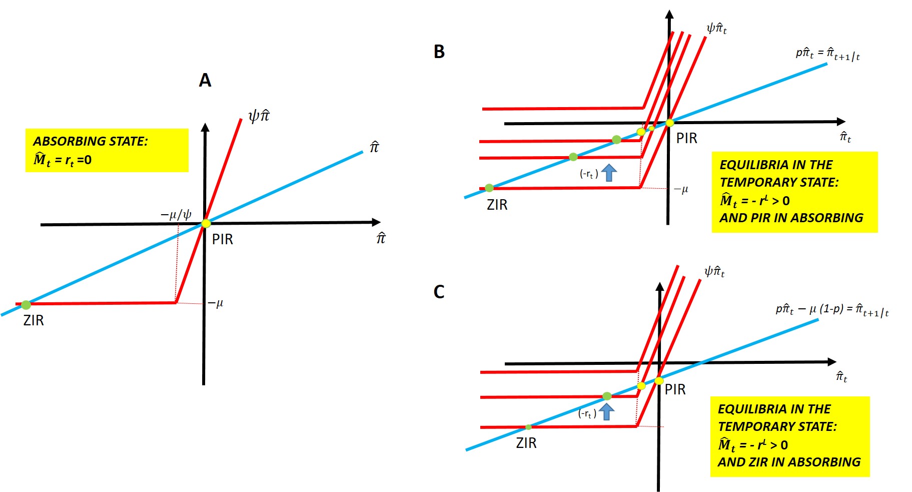
Figure 6: The possible equilibrium outcomes in Example ACS

Example ACS continued

To start with, consider the special case where $M_{t}$ satisfies Assumption 1. A corollary of Proposition 7 (with $q=1$ and $\sigma=\infty$) shows that the CC condition is satisfied if and only if $\psi<p$. Hence, for $\psi\geq p$ there will be up to 4 MSV solutions if the support of $M_{t}$ allows it. These are shown in Figure 6 and Table 2 for $\psi>1$, see Appendix A.6 for the derivation. The equilibrium typically used in the literature is the second one in Table 2: ZIR in the transitory and PIR in the absorbing state. This is a fairly intuitive choice in this simple case, but there is no clear choice in more general scenarios with no absorbing state and $k>2$.

Table 2: The four possible equilibria in Example ACS when $\psi>1$

Analytical Solution		Type of Equilibrium
$\hat{\pi}_{t}=\left\{\begin{array}[c]{ll}r^{L}\frac{p}{\psi-p}&\text{if }\hat{M}_{t}=-r^{L}\in\left(0,\mu\frac{\psi-p}{\psi p}\right)\\ 0&\text{if }\hat{M}_{t}=0\end{array}\right.$		(PIR, PIR)
$\hat{\pi}_{t}=\left\{\begin{array}[c]{ll}-r^{L}-\frac{\mu}{p},&\text{if }\hat{M}_{t}=-r^{L}\in\left(0,\mu\frac{\psi-p}{\psi p}\right)\\ 0&\text{if }\hat{M}_{t}=0\end{array}\right.$		(ZIR, PIR)
$\hat{\pi}_{t}=\left\{\begin{array}[c]{ll}\frac{pr^{L}-\left(1-p\right)\mu}{\psi-p},&\text{if }\hat{M}_{t}=-r^{L}\in\left(0,\mu\frac{\psi-1}{\psi}\right)\\ -\mu&\text{if }\hat{M}_{t}=0\end{array}\right.$		(PIR, ZIR)
$\hat{\pi}_{t}=\left\{\begin{array}[c]{ll}-r^{L}-\mu,&\text{if }\hat{M}_{t}=-r^{L}\in\left(0,\mu\frac{\psi-1}{\psi}\right)\\ -\mu,&\text{if }\hat{M}_{t}=0.\end{array}\right.$		(ZIR, ZIR)

To demonstrate the problem, we consider the case where $\hat{M}_{t}$ is described by a $k$-state Rouwenhorst (1995) approximation of an AR(1) process $\hat{M}_{t}=\rho\hat{M}_{t-1}+\sigma_{\varepsilon}\varepsilon_{t}$, with parameter values $\rho=0.9$ and $\sigma_{\varepsilon}=0.0007$, and we set $\psi=1.5$ and $\mu=2\log(1.005)$ following the calibration in ACS, so that the CC condition fails. Figure 7 reports the 8 MSV solutions corresponding to $k=3$. We notice that the first solution is at the ZIR for all values of the shock, while the last solution is the opposite, always at PIR. Unsurprisingly, those two solutions are linear in $\hat{M}_{t}.$ The remaining 6 solutions are non-linear and half of them are non-monotonic in $\hat{M}_{t}$. In Appendix A.7, we present results for $k>3$, showing that the number of MSV solutions increases with $k$. In all cases, two solutions correspond to ZIR-only and PIR-only equilibria. For any $k$, it is possible to impose restrictions on the support of the distribution of the shocks such that we are always at ZIR or always at PIR. ∎

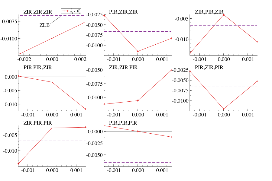
Figure 7: MSV solutions of model: $\hat{\pi}_{t|t+1}=max(-\mu,\psi\hat{\pi}_{t})+\hat{M}_{t+1|t}$, when $\mu=0.01$, $\psi=1.5$ and $\hat{M}_{t}$ follows a 3-state Markov Chain with mean 0, conditional st. dev. $\sigma=0.0007$, and autocorrelation $\rho=0.9$.

Example NK-TR continued

Consider again the NK model with $u_{t}=\nu_{t}=\psi_{x}=0$ and a Rouwenhorst approximation to an AR(1) process for the AD shock $\epsilon_{t}$. Figure 8 plots the decision rules for $\hat{\pi}_{t}$, $\hat{x}_{t}$ and $\hat{R}_{t}$, as functions of $\epsilon_{t}$, associated with various MSV equilibria of the model for $k=20,$ using the parameter values from Mertens and Ravn (2014), i.e., the left panel uses “MR2014 CD” and the right panel “MR2014 FD”. The graphs on the left report the four MSV equilibria arising from the calibration in which $\rho\sigma\lambda>\left(1-\rho\right)\left(1-\rho\beta\right)$. We notice that two of those equilibria have $\hat{\pi}_{t},\hat{x}_{t}$ respond positively to the AD shock, while the other two equilibria are exactly the opposite. The graphs on the right report the case $\rho\sigma\lambda<\left(1-\rho\right)\left(1-\rho\beta\right)$, where now only two MSV equilibria have been found, and they both have the property that the policy functions are increasing in the AD shock. Moreover, changing the parameters of the structural model or of the shocks yields a different number of solutions. For example, with a low variance of the shock and $\sigma=4$, the “MR2014 CD” case in Table 1 delivers 8 solutions. ∎

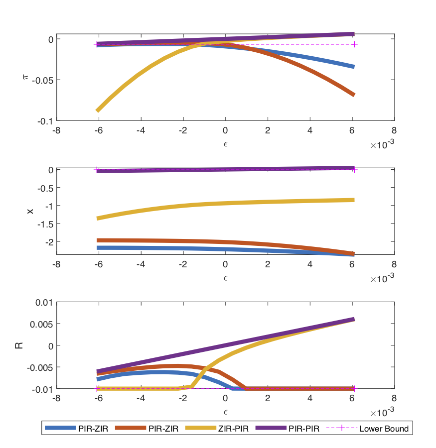
(a) Confidence-driven

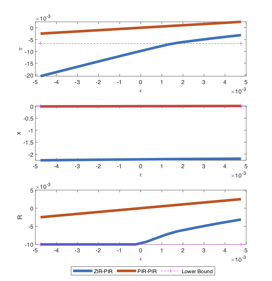
(b) Fundamental-driven

Figure 8: Decision Rules associated with different MSV solutions (equilibria) of the NK model, using parameters from Mertens and Ravn’s (2014) calibration shown in Table 1 and $k=20$. The figures on the left correspond to $\rho=0.7$ with $\sigma_{\epsilon}=0.0011$, while on the right $\rho=0.4$ and $\sigma_{\epsilon}=0.0014$.

4 Conclusions

This paper highlights a seemingly overlooked problem in rational expectation models with an occasionally binding constraint. The constraint might make the model incoherent or incomplete.

We propose a method for checking the coherency and completeness (CC) condition, that is, the existence and uniqueness of equilibria in piecewise linear DGSE models with a ZLB constraint based on Gourieroux et al. (1980). When applied to the typical NK model, this method shows that the CC condition generally violates the Taylor principle. Hence, the case typically analysed in the literature is either incoherent or incomplete. This raises two main issues future research should focus on when solving or estimating these models.

First, we have shown that there must be restrictions on the distribution of the shocks to ensure the existence of equilibria. These support restrictions are time-varying and, in the case of multiple shocks, their support is not rectangular, i.e., the shocks cannot be independent of each other. This raises a first question regarding the interpretation of these shocks: in what sense are they structural if they cannot be independent? A second related question regards the estimation of these models: what are the implications of these restrictions for the correct form of the likelihood?

Second, we have shown there are typically (many) more equilibria than currently reported in the literature. These findings raise questions about the properties of existing numerical solution algorithms, for example, which solutions among the many possible ones do they find and why.

We have not found a computationally feasible way to analyse coherency and completeness in forward-looking models in which the variables are continuously distributed. This problem is hard because of the infinite dimensionality induced by the rational expectation operator, and the fact that the computations required for discrete approximations are NP hard. This is an important challenge for future research.

Finally, our results highlight the role of unconventional monetary policy in ensuring coherency. An incoherent model cannot be an operational model of the economy. Hence, the need for support restrictions can be positively interpreted as an implicit need for a different policy reaction to catastrophic shocks to ensure the economy does not collapse. This suggests a direction for amending the basic NK model, by modelling monetary policy in such a way that, conditional on bad shocks hitting the economy and conventional interest rate policy being constrained by the ZLB, the use of unconventional monetary policies offers a route to solving the incoherency problem. This route is not only promising, but, even more importantly, realistic: central banks engaged in massive operations through unconventional monetary policy measures (beyond the standard interest rate policy) in response to the large negative shocks causing the Great Financial Crisis and the COVID-19 pandemic. Future work should also study whether it is possible to design fiscal policy to ensure equilibrium existence (e.g., Nakata and Schmidt, 2020). A takeaway from of our paper, therefore, is to warn that considering a ZLB constraint on monetary policy requires an explicit modelling of unconventional monetary policies (or some other mechanisms) to avoid incoherency.

Appendix A Appendix

A.1 Derivation of results in Subsection 2.1

Proof of Proposition 1.

Let $M^{t}=\left(M_{t},...,M_{0}\right)$ denote the history of $M_{t}.$ We consider fundamental solutions $f_{\pi_{t}}\left(M^{t}\right)$. Let $M_{L}^{t}=\left(\frac{e^{-r^{L}}}{r},...,\frac{e^{-r^{L}}}{r}\right)$ denote a path along which $M_{t}$ is in the transitory state. It follows that (with slight abuse of notation)

$$E\left(\left.\frac{M_{t+1}}{\pi_{t+1}}\right|M_{L}^{t}\right)=p\frac{\frac{e^{-r^{L}}}{r}}{f_{\pi_{t+1}}\left(\frac{e^{-r^{L}}}{r},M_{L}^{t}\right)}+\left(1-p\right)\frac{r^{-1}}{f_{\pi_{t+1}}\left(r^{-1},M_{L}^{t}\right)}.$$ (A1)

Next, if $M_{t+1}=r^{-1}$, we have $E\left(\left.\frac{M_{t+2}}{\pi_{t+2}}\right|M_{t+1}=r^{-1},M_{L}^{t}\right)\allowbreak=\frac{r^{-1}}{f_{\pi_{t+2}}\left(r^{-1},r^{-1},M_{L}^{t}\right)}$, so that after taking logs and re-arranging, (3) becomes

$$f_{\hat{\pi}_{t+2}}\left(0,0,\hat{M}_{L}^{t}\right)=\max\left\{-\mu,\psi f_{\hat{\pi}_{t+1}}\left(0,\hat{M}_{L}^{t}\right)\right\},$$ (A2)

where $f_{\hat{\pi}_{t}}\left(\cdot\right):=\log f_{\pi_{t}}\left(\cdot\right)-\log(\pi_{*})$, $\mu:=\log(r\pi_{*})$, and $\hat{M}_{t}:=\log M_{t}+\log r$, the latter being in log-deviation from its absorbing state. We have already established the support restriction $r\pi_{*}\geq 1$ in the main text after Proposition 1, which means $\mu\geq 0$. Because $\psi>1$, the difference equation (A2) has two steady states, $-\mu$ and $0$, corresponding to ZIR and PIR, respectively. Moreover, the ZIR steady state is stable, while the PIR is unstable. Therefore, for stable equilibria we must have that $f_{\hat{\pi}_{t+1}}\left(0,\hat{M}_{L}^{t}\right)\leq 0$, for if $f_{\hat{\pi}_{t+1}}\left(0,\hat{M}_{L}^{t}\right)>0$, $f_{\hat{\pi}_{t+s}}\left(0_{s\times 1},\hat{M}_{L}^{t}\right)$ will grow exponentially without bound. So, a stable fundamental solution must have $f_{\hat{\pi}_{t+1}}\left(0,\hat{M}_{L}^{t}\right)\leq 0,$ or equivalently $f_{\pi_{t+1}}\left(r^{-1},M_{L}^{t}\right)\leq\pi_{*}.$

Setting $f_{\pi_{t+1}}\left(r^{-1},M_{L}^{t}\right)=\bar{\pi}\leq\pi_{*}$ in (A1), substituting for $E\left(\left.\frac{M_{t+1}}{\pi_{t+1}}\right|M_{L}^{t}\right)$ in (3) and rearranging yields

$$\pi_{t+1}^{L}=\frac{\bar{\pi}p\max\left\{1,r\pi_{*}\left(\pi_{t}^{L}/\pi_{*}\right)^{\psi}\right\}e^{-r^{L}}}{r\bar{\pi}-\left(1-p\right)\max\left\{1,r\pi_{*}\left(\pi_{t}^{L}/\pi_{*}\right)^{\psi}\right\}},\quad\pi_{t}^{L}<\pi_{*}\left(\frac{\bar{\pi}/\pi_{*}}{1-p}\right)^{1/\psi},$$ (A3)

where $\pi_{t}^{L}:=f_{\pi_{t}}\left(M_{L}^{t}\right)$, for compactness of notation, and the bound on $\pi_{t}^{L}$ is required for $\pi_{t+1}^{L}$ to be positive. Take logs and define $\hat{\pi}_{t}^{L}:=\log\pi_{t}^{L}-\log\pi_{*}$, then (A3) can be written as

$$\hat{\pi}_{t+1}^{L}=\left\{\begin{array}[c]{ll}\log\frac{p\bar{\pi}/\pi_{*}}{r\bar{\pi}-1+p}-r^{L},&\hat{\pi}_{t}^{L}\leq-\frac{\mu}{\psi}\\ \log\frac{p\bar{\pi}/\pi_{*}}{\bar{\pi}/\pi_{*}-\left(1-p\right)e^{\psi\hat{\pi}_{t}^{L}}}+\psi\hat{\pi}_{t}^{L}-r^{L},&-\frac{\mu}{\psi}<\hat{\pi}_{t}^{L}<\bar{\hat{\pi}}_{t}^{L}=\frac{\log\bar{\pi}/\pi_{*}-\log\left(1-p\right)}{\psi}.\end{array}\right.$$ (A4)

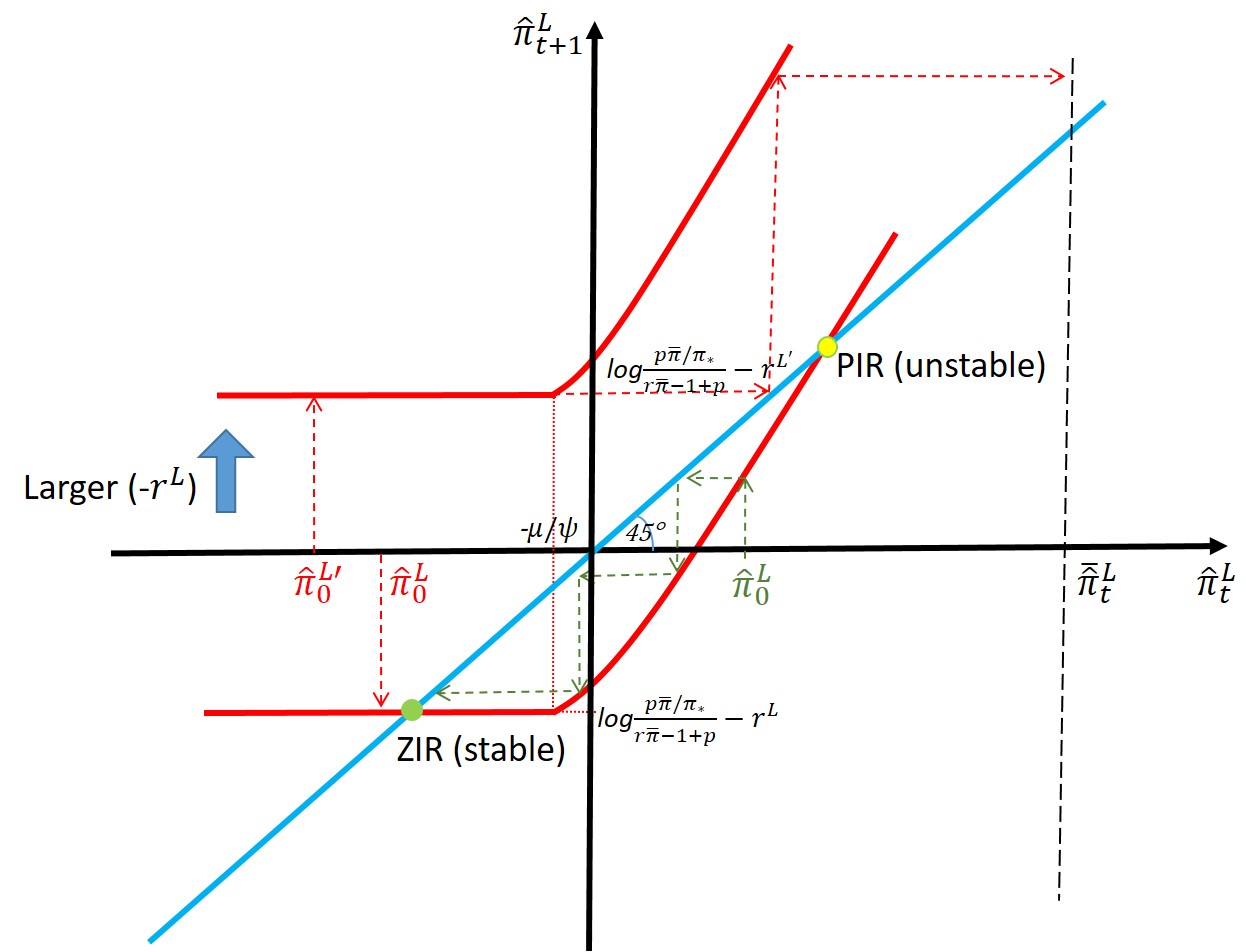
Figure 9: Plot of (A4) for different values of $-r^{L^{\prime}}>-r^{L}>0.$

Figure 9 plots (A4) against $\hat{\pi}_{t}^{L}$ together with the $45\mathrm{°}$ line. We distinguish two cases. The first case is when the curve intersects with the $45\mathrm{°}$ line, so that (A4) has two (generic) steady states. This happens when the kink in (A4) is below the $45\mathrm{°}$ line. Noting that the kink is given by $(\hat{\pi}_{t}^{L}=-\frac{\mu}{\psi};\allowbreak\hat{\pi}_{t+1}^{L}=\log\frac{p\bar{\pi}/\pi_{*}}{r\bar{\pi}-1+p}\allowbreak-r^{L})$, then the condition $\hat{\pi}_{t}^{L}>\hat{\pi}_{t+1}^{L}$ becomes

$$-r^{L}\leq-\frac{\mu}{\psi}-\log\frac{p\bar{\pi}/\pi_{*}}{r\bar{\pi}-1+p}\leq-\frac{\log(r\pi_{*})}{\psi}-\log\frac{p}{r\pi_{*}-1+p},$$ (A5)

where the second inequality holds because $-\log\frac{p\bar{\pi}/\pi_{*}}{r\bar{\pi}-1+p}$ is an increasing function of $\bar{\pi}\leq\pi_{*}$ and the definition of $\mu=-\log(r\pi_{*}).$ When the restriction (A5) on the support of the shock holds, then there clearly exist stable solutions to the model for arbitrary initial conditions $\hat{\pi}^{L}_{0}\leq\hat{\pi}^{PIR}$, where $\hat{\pi}^{PIR}$ is the high-inflation fixed point of the difference equation (A4).

Now consider the case when the support restriction (A5) does not hold. In this case, for any initial value $\hat{\pi}^{L}_{0}$ the solution of the difference equation (A4) will move along an explosive path while $\hat{\pi}^{L}_{t}$ is less than $\frac{\log\bar{\pi}/\pi_{*}-\log\left(1-p\right)}{\psi},$ and will eventually break down after a finite number of periods.

Finally, note how the transitory state resembles the simple case of the absorbing state in the main text, and Figure 9 parallels Figure 1. At $\bar{\pi}=\pi_{\ast},$ the support restrictions simply implies that $\hat{\pi}^{ZIR}=\ln\frac{p}{r\pi_{\ast}-1+p}-r^{L}<-\frac{\mu}{\psi}<0.$ So, for an equilibrium to exists the intercept of the ZIR part of the red line must be negative, as in Figure 1. ∎

Proof of Proposition 2.

Sunspot solutions $\pi_{t}$ may depend on $\varsigma_{t}$ and its lags. It is assumed that $\varsigma_{t}$ follows a first-order Markov chain, and so we may denote by $\pi_{t}^{\varsigma}$ the two different values that $\pi_{t}$ can take depending on the outcome of the sunspot shock. Letting $q_{\varsigma}:=\Pr(\varsigma_{t+1}=1|\varsigma_{t}=\varsigma)$, (3) becomes

$$1=\max\left\{r^{-1},\pi_{*}\left(\frac{\pi_{t}^{\varsigma_{t}}}{\pi_{*}}\right)^{\psi}\right\}\left(\frac{1-q_{\varsigma_{t}}}{\pi_{t+1}^{0}}+\frac{q_{\varsigma_{t}}}{\pi_{t+1}^{1}}\right)\qquad\varsigma_{t}=0,1.$$ (A6)

This is a system of nonlinear difference equations in $\pi_{t}^{\varsigma}$.

First, consider the case in which at least one of the initial values $\pi_{t}^{\varsigma_{t}}$ corresponds to a ZIR, which, wlog, we can set as $\left(\pi_{t}^{0}/\pi_{*}\right)^{\psi}\leq(r\pi_{*})^{-1}$, since the labelling of $\varsigma_{t}$ is arbitrary. Under this assumption, (A6) yields $r=\left(\frac{1-q_{0}}{\pi_{t+1}^{0}}+\frac{q_{0}}{\pi_{t+1}^{1}}\right),$ which we can solve for $\pi_{t+1}^{0}$ and substitute back into (A6) with $\varsigma_{t}=1$ to get

$$\pi_{t+1}^{1}=\frac{\max\left\{r^{-1},\pi_{*}\left(\pi_{t}^{1}/\pi_{*}\right)^{\psi}\right\}\left(q_{1}-q_{0}\right)}{1-q_{0}-r\max\left\{r^{-1},\pi_{*}\left(\pi_{t}^{1}/\pi_{*}\right)^{\psi}\right\}\left(1-q_{1}\right)}.$$

This has almost exactly the same shape as (A3) that is plotted in Figure 9. Hence, the same argument as above estabilishes the support restriction $r^{-1}\leq\pi_{*}$.

Second, suppose $\pi_{t}^{\varsigma_{t}}$ corresponds to a PIR for both $\varsigma_{t},$ i.e., $\left(\pi_{t}^{\varsigma_{t}}/\pi_{*}\right)^{\psi}>(r\pi_{*})^{-1}$. By the argument in the previous paragraph, if at any future date $\pi_{t+j}^{\varsigma_{t+j}}$ is a ZIR, then the support restriction for coherency $(r\pi_{*})^{-1}\leq 1$ applies. So, the only case to consider is when $\left(\pi_{t}^{\varsigma_{t}}/\pi_{*}\right)^{\psi}>(r\pi_{*})^{-1}$ for all $t$, i.e., the economy is always at a PIR. In this case, (A6) becomes $1=(\pi_{t}/\pi_{*})^{\psi}E_{t}\left(\pi_{*}/\pi_{t+1}\right),$ with the additional restriction $\pi_{t}>\pi_{*}(r\pi_{*})^{-1/\psi}$ for all $t.$ Because $\psi>1,$ this equation has the unique stable solution $\pi_{t}=\pi_{*}$ for all $t$ if and only if $r^{-1}\leq\pi_{*}$. ∎

A.2 Derivation of results in Subsection 2.2

A.2.1 Coefficients of the canonical form

Coefficients in Example NK-TR

$$A_{0} =\begin{pmatrix}1&-\lambda\\ 0&1\end{pmatrix},\quad A_{1}=\begin{pmatrix}1&-\lambda\\ \sigma\psi&1+\sigma\psi_{x}\end{pmatrix},\quad B_{0}=B_{1}=\begin{pmatrix}-\beta&0\\ -\sigma&-1\end{pmatrix},$$

$$C_{0} =\begin{pmatrix}-1&0&0&0\\ 0&-1&0&-\sigma\mu\end{pmatrix},\quad C_{1}=\begin{pmatrix}-1&0&0&0\\ 0&-1&\sigma&0\end{pmatrix},\quad D_{0}=D_{1}=0_{2\times 4},$$

$a=\left(\psi,\psi_{x}\right)^{\prime},$ $b=\left(0,0\right)^{\prime}$, $c=\left(0,0,1,\mu\right)^{\prime}$ and $d=0_{4\times 1}.$ ∎

Coefficients in Example NK-OP

$$A_{0} =\begin{pmatrix}1&-\lambda\\ 0&1\end{pmatrix},\quad A_{1}=\begin{pmatrix}1&-\lambda\\ \frac{\lambda}{\gamma}&1\end{pmatrix},\quad B_{0}=\begin{pmatrix}-\beta&0\\ -\sigma&-1\end{pmatrix},\quad B_{1}=\begin{pmatrix}-\beta&0\\ 0&0\end{pmatrix},$$

$$C_{0} =\begin{pmatrix}-1&0&0\\ 0&-1&-\sigma\mu\end{pmatrix},\quad C_{1}=\begin{pmatrix}-1&0&0\\ 0&0&0\end{pmatrix},\quad D_{0}=D_{1}=0_{2\times 3},$$

$a=\left(0,-\sigma^{-1}\right)^{\prime},$ $b=\left(1,\sigma^{-1}\right)^{\prime}$, $c=\left(0,\sigma^{-1},\mu\right)^{\prime}$ and $d=0_{3\times 1}.$ ∎

A.2.2 Proof of Proposition 3

In preparation for the proof of Proposition 3, we first establish a result that will be used in the proofs of both Propositions 3 and 7.

Proposition 9.

The NK-TR model given by (6) with $u_{t}=\nu_{t}=0$ and $\epsilon_{t}$ a two-state Markov Chain with transition Kernel $K=\begin{pmatrix}p&1-p\\ 1-q&q\end{pmatrix}$ can be written in the form $F(\mathbf{Y})=\kappa(\mathbf{X})$, where $\mathbf{Y}$ is a $2\times 1$ vector containing the values of $\hat{\pi}_{t}$ in each of the two states, and $F(\cdot)$ is the piecewise linear function (9) with

$$\mathcal{A}_{J_{1}}=Q+\lambda\sigma\left(\psi I-\frac{\psi_{x}}{\lambda}\left(I-\beta K\right)\right),$$ (PIR,PIR)

(ZIR,PIR)

(PIR,ZIR)

(ZIR,ZIR).

   (A7)

where $e_{i}$ is the unit vector with $1$ in position $i$,

$$Q:=I-K-\beta\left(I-K\right)K-\lambda\sigma K$$ (A8)

and

$$\det\mathcal{A}_{J_{1}}=\sigma^{2}\lambda^{2}\left(\psi-1+\frac{\beta-1}{\lambda}\psi_{x}\right)\left(\psi-\psi_{p,q,\beta,\sigma\lambda}-\psi_{x}\frac{\left(1+\beta\left(1-p-q\right)\right)}{\lambda}\right),$$

(A9)

where $\psi_{p,q,\beta,\sigma\lambda}$ is given in (16).

Proof.

Collect the $k=2$ states of $\epsilon_{t}$ in the vector $\epsilon=\left(\epsilon^{1},\epsilon^{2}\right)^{\prime}$ and denote the corresponding states of $\hat{\pi}_{t},\hat{x}_{t},\hat{R}_{t}$ along a MSV solution by 2-dimensional vectors $\hat{\pi},\hat{x}$ and $\hat{R},$ respectively, where $y=f\left(\epsilon\right)$ for some function $f\left(\cdot\right),$ and for each $y\in\left\{\hat{\pi},\hat{x},\hat{R}\right\}.$ Because the dynamics are exogenous and determined completely by $K$, we have $E\left(y_{t+1}|\epsilon_{t}=\epsilon^{i}\right)=e_{i}^{\prime}Ky$. Stacking the two conditioning states, we can write, with slight abuse of notation, $y_{t+1|t}=K\epsilon$. Substituting into (6a) with $u_{t}=0,$ we obtain

$$\hat{\pi}=\beta\overbrace{K\hat{\pi}}^{\hat{\pi}_{t+1|t}}+\lambda\hat{x}.$$ (A10)

Similarly, from (6b) we obtain

$$\hat{x}=\overbrace{K\hat{x}}^{\hat{x}_{t+1|t}}-\sigma\left(\hat{R}-K\hat{\pi}\right)+\epsilon.$$ (A11)

Combining the above two equations, we obtain

$$\left(I-K\right)\hat{\pi}=\beta\left(I-K\right)K\hat{\pi}-\lambda\sigma\left(\hat{R}-K\hat{\pi}\right)+\lambda\epsilon.$$

Substituting for $\hat{R}=\max\left\{-\mu\iota_{2},\psi\hat{\pi}+\psi_{x}\hat{x}\right\},$ obtained from (6c) with $\nu_{t}=0,$ and for $\hat{x}=\lambda^{-1}\left(I-\beta K\right)\hat{\pi},$ and rearranging we get:

$$Q\hat{\pi}=-\lambda\sigma\max\left\{-\mu\iota_{2},\left(\psi I-\frac{\psi_{x}}{\lambda}\left(I-\beta K\right)\right)\hat{\pi}\right\}+\lambda\epsilon.$$ (A12)

This yields (A7). The determinants (A9) were derived using straightforward algebraic calculations (performed using Scientific Workplace). ∎

Proof of Proposition 3.

Setting $\psi_{x}=0$ in (A9), we obtain

$$\det\mathcal{A}_{J_{1}}=\sigma^{2}\lambda^{2}\left(\psi-1\right)\left(\psi-\psi_{p,q,\beta,\sigma\lambda}\right)>0.$$

Since $\psi_{p,q,\beta,\sigma\lambda}\leq 1$, $\det\mathcal{A}_{J_{1}}>0$, so coherency requires $\psi_{p,q,\beta,\sigma\lambda}>0$ for $\det\mathcal{A}_{J_{4}}>0$ from (A9). However, in that case, from (A9) we get

$$\det\mathcal{A}_{J_{2}}=-\sigma^{2}\lambda^{2}\left(\psi_{p,q,\beta,\sigma\lambda}\left(\psi-1\right)+\psi\left(1-q\right)\left(1+\frac{1-\beta\left(p+q-1\right)}{\sigma\lambda}\right)\right)<0$$

because $\beta\left(p+q-1\right)<1$, violating the CC condition in the (GLM). Theorem. ∎

Extension to $\psi_{x}\neq 0$

In this case, the Taylor principle becomes

$$\psi+\frac{\beta-1}{\lambda}\psi_{x}>1.$$ (A13)

It is straightforward to show that the CC condition fails when (A13) holds for the absorbing case $q=1$. Using this constraint in (A9), we obtain

$$\det\mathcal{A}_{J_{2}}=-\det\mathcal{A}_{J_{4}}\left(\psi+\frac{\beta-1}{\lambda}\psi_{x}-1\right).$$

Thus, the two determinants must have opposite sign, violating the CC condition in the (GLM). Theorem.

It seems too complicated to prove this result analytically for $q<1$, but we have verified it numerically for all the parametrizations we considered (see the replication code provided).∎

A.2.3 Proof of Proposition 4

Next, we establish a result that will be used in the proof of Propositions 4.

Proposition 10.

The NK-OP model given by (6) with (6c) replaced by (7) with $u_{t}=\nu_{t}=\psi_{x}=0$ and $\epsilon_{t}$ a two-state Markov Chain with transition Kernel $K=\begin{pmatrix}p&1-p\\ 1-q&q\end{pmatrix}$ can be written in the form (9) with

$$\mathcal{A}_{J_{1}}=\left(1+\frac{\lambda^{2}}{\gamma}\right)I-\beta K,$$

       (A14)

and

$$\det\mathcal{A}_{J_{1}}=\frac{\left(\gamma\left(1-\beta\right)+\lambda^{2}\right)\left(\gamma\left(1+\left(1-p-q\right)\beta\right)+\lambda^{2}\right)}{\gamma^{2}},$$

     (A15)

Proof.

From (6b) and (7) we obtain

$$\hat{x}=\left\{\begin{array}[c]{ccc}K\hat{x}-\sigma\left(-\mu-K\hat{\pi}\right)+\epsilon,&\text{if }K\hat{\pi}+\frac{1}{\sigma}\left(K\hat{x}-\hat{x}+\epsilon\right)\leq-\mu&\text{(ZIR)}\\ -\frac{\lambda}{\gamma}\hat{\pi},&\text{if }K\hat{\pi}+\frac{1}{\sigma}\left(K\hat{x}-\hat{x}+\epsilon\right)>-\mu&\text{(PIR)}\end{array}\right.$$ (A16)

where the inequalities are element-wise. Substituting for $\hat{x}$ using (A10) yields

$$\left(I-\beta K\right)\hat{\pi}=\left\{\begin{array}[c]{cc}K\left(I-\beta K\right)\hat{\pi}-\lambda\sigma\left(-\mu-K\hat{\pi}\right)+\lambda\epsilon,&\text{(ZIR)}\\ -\frac{\lambda^{2}}{\gamma}\hat{\pi},&\text{(PIR)}\end{array}\right.$$

where ZIR occurs if and only if $K\hat{\pi}+\frac{1}{\lambda\sigma}\left(\left(K-I\right)\left(I-\beta K\right)\hat{\pi}+\lambda\epsilon\right)\leq-\mu$ (element-wise). Thus, for PIR,PIR we have

$$\mathcal{A}_{J_{1}}=\left(1+\frac{\lambda^{2}}{\gamma}\right)I-\beta K$$

For ZIR,PIR, we have

$$\mathcal{A}_{J_{2}}=I-\beta K-e_{1}e_{1}^{\prime}\left(K\left(I-\beta K\right)+\lambda\sigma K\right)+\frac{\lambda^{2}}{\gamma}e_{2}e_{2}^{\prime},$$

and PIR,ZIR can be obtained symmetrically. For ZIR,ZIR, we have

$$\mathcal{A}_{J_{4}}=I-\beta K-\left(K\left(I-\beta K\right)+\lambda\sigma K\right)=Q.$$

This yields (A7). Finally, it is straightforward to verify (A15). ∎

Proof of Proposition 4.

First, observe that $\det\mathcal{A}_{J_{1}}>0$ holds for all admissible values of the parameters $\beta,p,q\in\left[0,1\right]$, and $\gamma,\lambda>0$, since $\gamma\left(1-\beta\right)+\lambda^{2}>0$ and $(1\allowbreak+(1-\allowbreak p-q)\beta)\geq 0$. Therefore, when $\theta>1$ ($\psi_{p,1,\beta,\sigma\lambda}<0$), the CC condition cannot hold because $\det\mathcal{A}_{J_{4}}<0$. Turning to the case $\theta<1$ ($\psi_{p,1,\beta,\sigma\lambda}>0$) we immediately notice that both $\det\mathcal{A}_{J_{2}}$ and $\det\mathcal{A}_{J_{3}}$ are negative, since the terms in the numerator of the fractions are all positive. ∎

A.2.4 Proof of Proposition 5

We first look at the absorbing (or steady) state, where $\epsilon_{t}=0.$ Then, we need to solve

$$\ \hat{\pi}=\frac{\lambda}{1-\beta}\hat{x}\quad AS\quad;\quad\hat{\pi}=\max\left\{-\mu,\psi\hat{\pi}\right\}=\max\left\{\begin{array}[c]{c}\psi\frac{\lambda}{1-\beta}\hat{x}\quad AD^{TR}\\ -\mu\qquad AD^{ZLB}\end{array}.\right.$$ (A17)

This is depicted in Figure 10. It is immediately obvious that the necessary support restriction for existence of a solution is $\mu\geq 0,$ i.e., $\left(r\pi_{\ast}\right)^{-1}\leq 1.$ When this holds, there are two possible solutions: 1) PIR: $(\hat{\pi},\hat{x},\hat{R})=(0,0,0)$; and 2) ZIR: $(\hat{\pi},\hat{x},\hat{R})=(-\mu,-\mu\frac{(1-\beta)}{\lambda},-\mu)$.

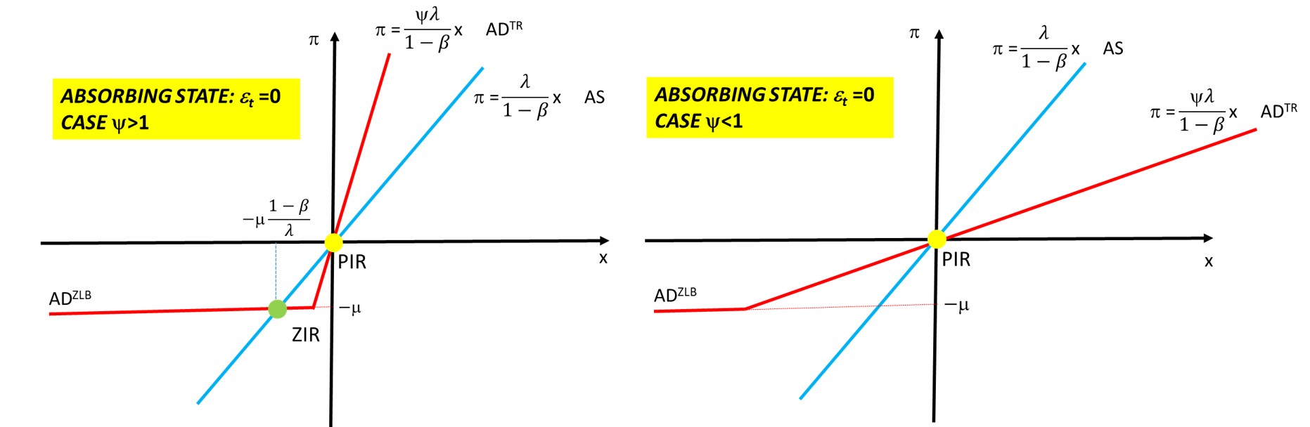
Figure 10: The absorbing state in the NK-TR model

Next, turn to the transitory state. Here, there are four possibilities depending on the value of $\theta$, and the equilibrium in the absorbing state. These are depicted in Figure 11. The derivations of those cases is as follows.

The temporary state lasts for a random time $T$, after which the economy jumps to the absorbing state, because the model is completely forward-looking with no endogenous persistence. In the transitory state $\epsilon_{t}=-\sigma\hat{M}_{t+1|t}=\sigma pr^{L}<0$, the equilibrium will be ($\hat{\pi}^{L},\hat{x}^{L}$) and with probability $(1-p)$ we are back in the absorbing state. The latter can be a PIR one or a ZIR one.

Figure 11: The temporary state in the NK model when $\psi>1$.

When the absorbing state is PIR, the system becomes

$$\hat{\pi}^{L} =\frac{\lambda}{1-\beta p}\hat{x}^{L}\hskip 70.0001ptAS$$ (A18)

$$\hat{\pi}^{L} =\left\{\begin{array}[c]{c}\frac{1-p}{\sigma\left(p-\psi\right)}\hat{x}^{L}+\frac{p(-r^{L})}{\left(p-\psi\right)}\qquad AD^{TR}\hskip 20.00003pt\text{ for }\pi\geq-\frac{\mu}{\psi}\\ \frac{1-p}{\sigma p}\hat{x}^{L}-\frac{\mu}{p}+(-r^{L})\qquad AD^{ZLB}\hskip 10.00002pt\text{ for }\pi\leq-\frac{\mu}{\psi}\end{array}\right.$$ (A21)

These curves are plotted in the top row of Figure 11 for the cases $\theta>1$ on the left, i.e., panel (a), where $AS$ is flatter than $AD^{ZLB}$, and $\theta<1$ on the right, i.e., panel (b), where $AS$ is steeper than $AD^{ZLB}.$

When the absorbing state is ZIR, instead, expectations in the temporary equilibrium are different, so the system to solve for becomes

$$\hat{\pi}^{L} =\frac{\lambda}{1-\beta p}\hat{x}^{L}-\frac{\beta\mu(1-p)}{1-\beta p}\hskip 90.00014ptAS$$ (A22)

$$\hat{\pi}^{L} =\left\{\begin{array}[c]{c}\hat{x}^{L}\frac{(1-p)}{\sigma\left(p-\psi\right)}+\frac{p(-r^{L})}{p-\psi}+{\frac{\mu(1-p)}{p-\psi}\left[\frac{(1-\beta)}{\lambda\sigma}+1\right]}\quad AD^{TR}\hskip 10.00002pt\text{ for }\pi\geq-\frac{\mu}{\psi}\\ \hat{x}^{L}\frac{1-p}{\sigma p}-\frac{\mu}{p}-r^{L}+\frac{\mu(1-p)}{p}\left[\frac{(1-\beta)}{\lambda\sigma}+1\right]\qquad AD^{ZLB}\text{ for }\pi\leq-\frac{\mu}{\psi}\end{array}\right.$$ (A25)

These curves are plotted in the bottom row of Figure 11 for the cases $\theta>1$ on the left, i.e., panel (c), where $AS$ is flatter than $AD^{ZLB}$, and $\theta<1$ on the right, i.e., panel (d), where $AS$ is steeper than $AD^{ZLB}.$

Inspection of the graphs on the left of Figure 11, where $\theta>1$ for PIR absorbing (panel (a)) and ZIR absorbing (panel (c)) shows there is always a solution in both cases. We therefore conclude that when $\theta>1,$ the only necessary support restriction is $\left(r\pi_{\ast}\right)^{-1}\leq 1$ for existence of an equilibrium in the absorbing state. This proves (11a).

Next, turn to the case $\theta<1.$ Now it is clear that a further support restriction is needed on the value of the shock in the transitory state. The cutoff can be computed by finding the point where the $AD$ and $AS$ curves intersect at the kink of $AD$. There are two different points for the cases in Figure 11: panel (b), PIR absorbing and panel (d), ZIR absorbing. From inspection, it is clear that the former is the least stringent condition, so it suffices to focus on that. Specifically, we equate (A18) with (A21) at $\hat{\pi}^{L}=-\frac{\mu}{\psi}$ to find the value of the shock $r^{L}=\bar{r}^{L}$ such that the equations have a solution for all $-r^{L}\leq-\bar{r}^{L}.$ Hence, the cutoff can be found by solving:

$$-\frac{\mu}{\psi}\frac{1-\beta p}{\lambda}=\sigma\frac{-\left(p-\psi\right)\frac{\mu}{\psi}+p\bar{r}^{L}}{1-p},$$

which yields

$$-\bar{r}^{L}=\frac{\mu}{\psi}\frac{\left(1-\beta p\right)\left(1-p\right)}{p\lambda\sigma}-\frac{\left(p-\psi\right)}{p}\frac{\mu}{\psi}=\mu\left(\frac{\psi-p}{\psi p}+\frac{\theta}{\psi}\right),$$

which proves (11b). ∎

A.2.5 Proof of Proposition 6

We first look at the absorbing (or steady) state, where $\epsilon_{t}=0.$ Then, the system to solve is

$$\ \hat{\pi}=\frac{\lambda}{1-\beta}\hat{x}\quad AS\quad;\quad\hat{\pi}=\max\left\{\begin{array}[c]{c}-\frac{\gamma}{\lambda}\hat{x}\quad AD^{OP}\\ -\mu\qquad AD^{ZLB}\end{array}.\right.$$ (A26)

This is depicted in Figure 12. In contrast with the NK-TR case, there are two inequalities to satisfy: the ZLB and the slackness condition on optimal policy, i.e., (7). In the NK-TR case, there is only the former inequality, while the Taylor rule is expressed as equality, thus graphically a feasible point above the ZLB needs to be on the $AD^{TR}$ line. Here instead, a feasible point can be below the first order conditions for optimal policy. In Figure 12 both the PIR and the ZIR are feasible steady states. The PIR equilibrium is feasible because it satisfies the ZLB constraint, i.e., is above the horizontal $AD^{ZLB}$ ZLB line. The ZIR equilibrium is feasible because it satisfies the slackness condition on the first order conditions on optimal policy constraint, i.e., is below the $AD^{OP}$ line. It is immediately obvious that the necessary support restriction for existence of a solution is $\mu\geq 0,$ i.e., $r^{-1}\leq\pi_{\ast}$. When this holds, there are two possible solutions: 1) PIR: $(\hat{\pi},\hat{x},\hat{R})=(0,0,0)$; and 2) ZIR: $(\hat{\pi},\hat{x},\hat{R})=(-\mu,-\mu\frac{(1-\beta)}{\lambda},-\mu)$.

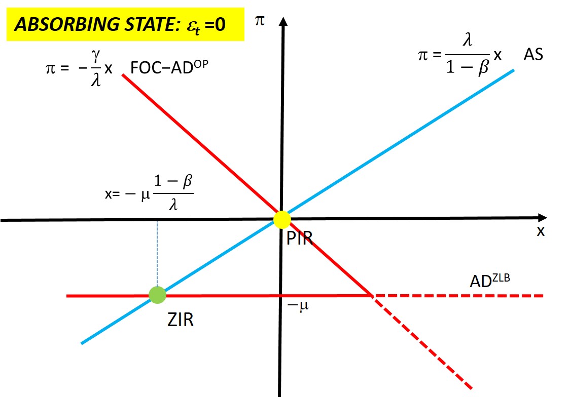
Figure 12: The absorbing state in the NK-OP model.

Next, turn to the transitory state. Here, there are four possibilities depending on the value of $\theta,$ and the equilibrium in the absorbing state. These are depicted in Figure 13. The derivations of those cases is as follows.

As before, the temporary state lasts for a random time $T$, after which the economy jumps to the absorbing state, because the model is completely forward-looking with no endogenous persistence. In the transitory state $\epsilon_{t}=-\sigma\hat{M}_{t+1|t}=\sigma pr^{L}<0$, the equilibrium will be ($\hat{\pi}^{L},\hat{x}^{L}$) and with probability $(1-p)$ we are back in the absorbing state. The latter can be a PIR one or a ZIR one.

Figure 13: The temporary state in the NK-OP model.

When the absorbing state is PIR and the ZLB does not bind, the system becomes

$$\hat{\pi}^{L} =\frac{\lambda}{1-\beta p}\hat{x}^{L}\qquad AS$$

$$\hat{\pi}^{L} =-\frac{\gamma}{\lambda}\hat{x}^{L}\qquad AD^{OP}$$

$$\hat{\pi}^{L} >\hat{\pi}^{L,ZLB}=\hat{x}^{L}\frac{1-p}{\sigma p}-\frac{\mu}{p}-r^{L}\qquad AD^{ZLB}$$ (A27)

When the absorbing state is PIR and the ZLB binds, then $\hat{\pi}^{L}=\hat{\pi}^{L,ZLB}$ and $\hat{\pi}^{L,ZLB}$ needs to be smaller than the one the central bank would have chosen to satisfy the first order conditions: $\hat{\pi}^{L}\leq-\frac{\gamma}{\lambda}\hat{x}^{L}.$ The system becomes

$$\hat{\pi}^{L} =\frac{\lambda}{1-\beta p}\hat{x}^{L}\qquad AS$$

$$\hat{\pi}^{L} \leq-\frac{\gamma}{\lambda}\hat{x}^{L}\qquad AD^{OP}$$

$$\hat{\pi}^{L} =\hat{\pi}^{L,ZLB}=\hat{x}^{L}\frac{1-p}{\sigma p}-\frac{\mu}{p}-r^{L}\qquad AD^{ZLB}$$ (A28)

The inequality in (A27) states that the equilibrium is above the $AD^{ZLB};$ the inequality (A28) states you that the equilibrium is below the $AD^{OP}.$ These curves are plotted in the top row of Figure 13 for the cases $\theta>1$ on the left, i.e., panel (a), where $AS$ is flatter than $AD^{ZLB}$, and $\theta<1$ on the right, i.e., panel (b), where $AS$ is steeper than $AD^{ZLB}.$ An increase in $-r^{L}$, i.e., an increase in the absolute value of the negative discount factor shock, shifts the $AD^{ZLB}$ upwards. In both cases, there exists a threshold level of $(-r^{L})=\frac{\mu}{p}$ such that the PIR coincides with the ZIR, that is, such that the intersection between $AS$ and $AD^{OP}$ coincides with the intersection between $AS$ and $AD^{ZLB}$. Hence:

(i) when $\theta>1$, there is unique equilibrium that is a ZIR if $-pr^{L}>\mu$ and a PIR if $-pr^{L}<\mu$;

(ii) when $\theta<1$, there is no equilibrium if $-pr^{L}>\mu$ and 2 equilibria (both a ZIR and a PIR) if $-pr^{L}<\mu$.

When the absorbing state is ZIR, instead, expectations in the temporary equilibrium are different, and given by

$$E_{t}\left(\hat{\pi}_{t+1}\right) =p\hat{\pi}^{L}-\mu(1-p),$$

$$E_{t}\left(\hat{x}_{t+1}\right) =p\ast(\hat{x}^{L})+(1-p)\ast\left(-\mu\frac{(1-\beta)}{\lambda}\right)=p\hat{x}^{L}-\mu\frac{(1-\beta)(1-p)}{\lambda}.$$

When the absorbing state is ZIR and the ZLB does not bind, the system becomes

$$\hat{\pi}^{L} =\frac{\lambda}{1-\beta p}\hat{x}^{L}-\frac{\beta\mu(1-p)}{1-\beta p}\qquad AS$$

$$\hat{\pi}^{L} =-\frac{\gamma}{\lambda}\hat{x}^{L}\qquad AD^{OP}$$

$$\hat{\pi}^{L} >\hat{\pi}^{L,ZLB}=\hat{x}^{L}\frac{1-p}{\sigma p}-r^{L}+\mu\left(\frac{1-p}{p}\frac{1-\beta}{\sigma\lambda}-1\right)\qquad AD^{ZLB}$$

In the ZLB, instead

$$\hat{\pi}^{L} =\frac{\lambda}{1-\beta p}\hat{x}^{L}-\frac{\beta\mu(1-p)}{1-\beta p}\text{ \ \ \ \ \ }AS$$

$$\hat{\pi}^{L} \leq-\frac{\gamma}{\lambda}\hat{x}^{L}\text{ \ \ \ \ \ \ \ }AD^{OP}$$

$$\hat{\pi}^{L} =\hat{\pi}^{L,ZLB}=\hat{x}^{L}\frac{1-p}{\sigma p}-r^{L}+\mu\left(\frac{1-p}{p}\frac{1-\beta}{\sigma\lambda}-1\right)\text{ \ \ \ \ \ \ \ }AD^{ZLB}$$

These curves are plotted in the bottom row of Figure 13 for the cases $\theta>1$ on the left, i.e., panel (c), where $AS$ is flatter than $AD^{ZLB}$, and $\theta<1$ on the right, i.e., panel (d), where $AS$ is steeper than $AD^{ZLB}.$ In both cases, $r^{L}$ shifts the $AD^{ZLB}$ and there exists a threshold level of $(-r^{L})=\overline{\left(-r^{L}\right)}>\frac{\mu}{p}$ such that the PIR coincides with the ZIR, that is, such that the intersection between $AS$ and $AD^{OP}$ coincides with the intersection between $AS$ and $AD^{ZLB}$. Hence:

(i) when $\theta>1$, there is unique equilibrium that is a ZIR if $(-r^{L})>\overline{\left(-r^{L}\right)}$ and a PIR if $(-r^{L})<\overline{\left(-r^{L}\right)}$;

(ii) when $\theta<1$, there is no equilibrium if $(-r^{L})>\overline{\left(-r^{L}\right)}$ and 2 equilibria (both a ZIR and a PIR) if $(-r^{L})<\overline{\left(-r^{L}\right)}$.

When $\theta>1$, thus, for PIR absorbing (panel (a)) and ZIR absorbing (panel (c)) there is always a solution in both cases. We therefore conclude that when $\theta>1,$ the only necessary support restriction is $r^{-1}\leq\pi_{\ast}$ for existence of an equilibrium in the absorbing state. This proves (12a). When $\theta<1$, as evident from the graph and easy to prove, $\overline{\left(-r^{L}\right)}<\frac{\mu}{p}$. Thus, the relevant support restriction for coherency is given by $-r^{L}<\mu/p$, which is (12b). ∎

A.2.6 Existence of sunspot equilibria in NK-TR model

Consider the NK-TR model in Proposition 5 with the additional restriction $\epsilon_{t}=0$ and suppose there is a sunspot shock $\varsigma_{t}\in\left\{0,1\right\}$ with transition matrix $K$. In this case, the vector of exogenous state variables in the canonical representation (5) can be written as $X_{t}=\left(1,\varsigma_{t}\right)^{\prime}$. The model can be written as a piecewise linear system of equations $F\left(\mathbf{Y}\right)=\kappa,$ where $F\left(\cdot\right)$ is given by (9) with $\mathcal{A}_{J}$ given by Proposition 9 as before, since the sunspot shock affects the expectations in exactly the same way as a real shock would have. The RHS terms $\kappa$ can be obtained from (A12) with $\psi_{x}=0$ and $\epsilon=0$, that is,

$$\kappa_{J_{1}}=0_{2\times 1},$$ (PIR,PIR)

(ZIR,PIR)

(PIR,ZIR)

(ZIR,ZIR).

The four potential equilibria (solutions) are given by $\hat{\pi}_{J}:=\mathcal{A}_{J}^{-1}\kappa_{J},$ i.e.,

$$\hat{\pi}_{J_{1}}=0_{2\times 2},$$ (PIR,PIR)

(ZIR,PIR)

(PIR,ZIR)

(ZIR,ZIR),

(A29)

where we used the definitions

$$a_{q} :=\left(q-1\right)\left(\beta\left(1-p-q\right)+\sigma\lambda+1\right)\leq 0$$

$$a_{p} :=\left(p-1\right)\left(\beta\left(1-p-q\right)+\sigma\lambda+1\right)\leq 0,$$

for compactness, and the fact that

$$a_{p}+a_{q}+\sigma\lambda = \left(q-1\right)\left(\beta\left(1-p-q\right)+\sigma\lambda+1\right)+$$

$$\left(p-1\right)\left(\beta\left(1-p-q\right)+\sigma\lambda+1\right)+\sigma\lambda$$

$$= \left(p+q-2\right)\left(\beta\left(1-p-q\right)+1\right)+\left(p+q-1\right)\sigma\lambda$$

$$= \sigma\lambda\psi_{p,q,\beta,\sigma\lambda}.$$

Note that the PIR,PIR and ZIR,ZIR equilibria are actually sunspotless in the sense that they are completely independent of the sunspot process. (They don’t depend on $K,$ i.e., $p,q$). This is perfectly intuitive, because the sunspot would be effectively choosing over two identical outcomes in each state. For existence of any of those equlibria, the support restirction is $\mu\geq 0$. So, it remains to show that there is no weaker condition that can support any of the other two equilibria ZIR,PIR or PIR,ZIR. That is, we need to check if any of the two sets of inequalities:

$$\begin{pmatrix}\frac{\left(a_{q}+\sigma\lambda-\sigma\lambda\psi\right)\mu}{\psi a_{p}+\sigma\lambda\left(\psi-\psi_{p,q,\beta,\sigma\lambda}\right)}\leq-\frac{\mu}{\psi}\\ \frac{a_{q}\mu}{\psi a_{p}+\sigma\lambda\left(\psi-\psi_{p,q,\beta,\sigma\lambda}\right)}>-\frac{\mu}{\psi}\end{pmatrix}\text{\quad or\quad}\begin{pmatrix}\frac{a_{p}\mu}{\psi a_{q}+\sigma\lambda\left(\psi-\psi_{p,q,\beta,\sigma\lambda}\right)}>-\frac{\mu}{\psi}\\ \frac{\left(a_{p}+\sigma\lambda-\sigma\lambda\psi\right)\mu}{\psi a_{q}+\sigma\lambda\left(\psi-\psi_{p,q,\beta,\sigma\lambda}\right)}\leq-\frac{\mu}{\psi}\end{pmatrix}$$

can be satisfied when $\mu<0$.

Assuming $\mu<0$ and cancelling out $\mu,$ we have

$$\begin{pmatrix}\frac{\left(a_{q}+\sigma\lambda-\sigma\lambda\psi\right)}{\psi a_{p}+\sigma\lambda\left(\psi-\psi_{p,q,\beta,\sigma\lambda}\right)}\geq-\frac{1}{\psi}\\ \frac{a_{q}}{\psi a_{p}+\sigma\lambda\left(\psi-\psi_{p,q,\beta,\sigma\lambda}\right)}<-\frac{1}{\psi}\end{pmatrix}\text{\quad or\quad}\begin{pmatrix}\frac{a_{p}}{\psi a_{q}+\sigma\lambda\left(\psi-\psi_{p,q,\beta,\sigma\lambda}\right)}<-\frac{1}{\psi}\\ \frac{\left(a_{p}+\sigma\lambda-\sigma\lambda\psi\right)}{\psi a_{q}+\sigma\lambda\left(\psi-\psi_{p,q,\beta,\sigma\lambda}\right)}\geq-\frac{1}{\psi}\end{pmatrix}.$$ (A30)

Given that $a_{p}\leq 0$ and $a_{q}\leq 0,$ the bottom inequality on the LHS and the top inequality on the RHS both imply that $\psi a_{p}+\sigma\lambda\left(\psi-\psi_{p,q,\beta,\sigma\lambda}\right)>0$ and $\psi a_{q}+\sigma\lambda\left(\psi-\psi_{p,q,\beta,\sigma\lambda}\right)>0$, respectively. Then, in a ZIR,PIR equilibrium, the top inequality on the left of (A30) implies

$$\psi\left(a_{q}+a_{p}+\sigma\lambda-\sigma\lambda\psi\right) \geq -\sigma\lambda\left(\psi-\psi_{p,q,\beta,\sigma\lambda}\right),\quad\text{or}$$ (A31)

$$-\psi\sigma\lambda\left(\psi-\psi_{p,q,\beta,\sigma\lambda}\right) \geq -\sigma\lambda\left(\psi-\psi_{p,q,\beta,\sigma\lambda}\right),$$

which cannot hold, since $\psi>1$ and $\psi_{p,q,\beta,\sigma\lambda}\leq 1$. An entirely symmetric argument can be used to rule out a PIR,ZIR – the top inequality on the RHS of (A30) also leads to (A.2.6).

A.2.7 Relationship to Nakata and Schmidt (2019, Proposition 1)

The model in Nakata and Schmidt (2019) (henceforth NS) corresponds to (6a) with $u_{t}=0,$ (6b) with $\epsilon_{t}=-\sigma\hat{M}_{t+1|t}$ and (7). They denote their AD shock as $r_{t}^{n}:=\mu-\hat{M}_{t+1|t},$ in our notation, and assume that it follows a two-state Markov process with support $\left\{r_{L}^{n},r_{H}^{n}\right\},$ where $r_{L}^{n}<0<r_{H}^{n},$ and transition probabilities $\Pr\left(r_{t+1}^{n}=r_{L}^{n}|r_{t}^{n}=r_{j}^{n}\right)=p_{j}$ for $j\in\left\{L,H\right\}.$ This translates in our notation to $0>r_{L}^{n}=\mu+pr^{L},$ i.e., $-r^{L}p>\mu,$ and $0<r_{H}^{n}=\mu,$ i.e., $r^{-1}<\pi_{\ast}.$ The transition probabilities are in our notation $p_{L}=p$ and $p_{H}=1-q.$ When the ‘high’ state is absorbing ($q=1$), we have $p_{H}=0$ in their notation.

Specializing to the case $p_{H}=0,$ NS Proposition 1 states that an equilibrium exists if and only if the following condition holds

$$p\leq p_{L}^{\ast}\text{ \ \ and \ \ }0\leq p_{H}^{\ast},$$ (A32)

where

$$p_{L}^{\ast} =\frac{-q_{1}+\sqrt{q_{1}^{2}-4q_{2}q_{0}}}{2q_{2}},$$

$$q_{0} =-\left(\lambda^{2}+\gamma\left(1-\beta\right)\right)\frac{1}{\sigma\lambda}<0,$$

$$q_{1} =\left(\lambda^{2}+\gamma\left(1-\beta\right)\right)\left(\frac{1+\beta}{\sigma\lambda}+1\right)=-q_{0}\left(1+\beta+\sigma\lambda\right)>0,$$

$$q_{2} =-\left(\lambda^{2}+\gamma\left(1-\beta\right)\right)\frac{\beta}{\sigma\lambda}=\beta q_{0}<0,$$

so that

$$p_{L}^{\ast} =\frac{-q_{1}+\sqrt{q_{1}^{2}-4\beta q_{0}^{2}}}{2\beta q_{0}}=\frac{q_{0}\left(1+\beta+\sigma\lambda\right)-q_{0}\sqrt{\left(1+\beta+\sigma\lambda\right)^{2}-4\beta}}{2\beta q_{0}}$$

$$=\frac{1+\beta+\sigma\lambda-\sqrt{\left(1+\beta+\sigma\lambda\right)^{2}-4\beta}}{2\beta},$$ (A33)

and

$$p_{H}^{\ast} =\frac{-\phi_{1}-\sqrt{\phi_{1}^{2}-4\phi_{2}\phi_{0}}}{2\phi_{2}},$$ (A34)

$$\phi_{0} =-\left(\frac{1-p}{\sigma\lambda}\left(1-\beta p\right)-p\right)\frac{\mu}{\mu+pr^{L}}>0,$$

$$\phi_{1} =-\frac{1-\beta p+\left(1-p\right)\beta\frac{\mu}{\mu+pr^{L}}}{\sigma\lambda}-\frac{\lambda^{2}+\left(1-\beta\frac{\mu}{\mu+pr^{L}}\right)\gamma}{\lambda^{2}+\gamma\left(1-\beta\right)},$$

$$\phi_{2} =-\frac{\beta}{\sigma\lambda}<0.$$ (A35)

Substituting for $p_{L}^{\ast}$ in the first inequality in (A32) using (A33), we obtain

$$p<\frac{1+\beta+\sigma\lambda-\sqrt{\left(1+\beta+\sigma\lambda\right)^{2}-4\beta}}{2\beta}.$$ (A36)

This is equivalent to the condition $\theta>1$ in (12a). Specifically, note that $\theta=\frac{\left(1-p\right)\left(1-\beta p\right)}{\sigma\lambda p}>1$ is equivalent to

$$\left(1-p\right)\left(1-\beta p\right)-\sigma\lambda p>0.$$ (A37)

The discriminant of the quadratic equation $\left(1-p\right)\left(1-\beta p\right)-\sigma\lambda p=0$ is $\left(1+\beta+\sigma\lambda\right)^{2}-4\beta=\left(1-\beta\right)^{2}+2\sigma\lambda+\sigma^{2}\lambda^{2}+2\sigma\beta\lambda>0,$ so the equation has real roots $p_{1}\leq p_{2}$ given by

$$p_{1}=\frac{1+\beta+\sigma\lambda-\sqrt{\left(1+\beta+\sigma\lambda\right)^{2}-4\beta}}{2\beta},\ p_{2}=\frac{1+\beta+\sigma\lambda+\sqrt{\left(1+\beta+\sigma\lambda\right)^{2}-4\beta}}{2\beta}.$$

Thus, $\theta>1$ is equivalent to $p<p_{1}=p_{L}^{\ast},$ which is NS’s condition (A36).

Next, turn to the second inequality ($p_{H}^{\ast}\geq 0$) in (A32). From (A34) and (A35), this is equivalent to

$$-\phi_{1}\leq\sqrt{\phi_{1}^{2}-4\phi_{2}\phi_{0}}.$$

The inequality is obviously satisfied for $\phi_{1}>0,$ and therefore, it is only a restriction on how negative $\phi_{1}$ can be. In particular, it cannot fall below $-\sqrt{\phi_{1}^{2}-4\phi_{2}\phi_{0}},$ so, equivalently, when $\phi_{1}<0,$ we must have $\left|\phi_{1}\right|\leq\sqrt{\phi_{1}^{2}-4\phi_{2}\phi_{0}}$, which is clearly equivalent to $\phi_{2}\phi_{0}\leq 0$. Hence, the second condition of NS is equivalent to

$$\phi_{2}\phi_{0}=\frac{\beta}{\sigma\lambda}\left(\frac{\left(1-p\right)\left(1-\beta p\right)}{\sigma\lambda}-p\right)\frac{\mu}{\mu+pr^{L}}=\frac{\beta p\left(\theta-1\right)}{\sigma\lambda}\frac{\mu}{\mu+pr^{L}}\leq 0.$$

Since NS assumed $\mu+pr^{L}<0$ and $\mu>0,$ it must be that $\theta>1$. So, under NS’s restrictions on the support $r_{L}^{n}<0<r_{H}^{n},$ the condition (A32) in NS Proposition 1 is equivalent to $\theta>1$ in our Proposition 6.

A.3 Derivation of results in Subsection 2.4

Proof of Proposition 7.

Proposition 9 expresses the model in the form (9) and gives $\det\mathcal{A}_{J_{i}},$ $i=1,...,4$. We need to find the range of parameters for which all $\det\mathcal{A}_{J_{i}}$ are of the same sign. Inspection of (A9) shows we need to consider the following two cases.

Case $\psi_{p,q,\beta,\sigma\lambda}>0$.

For CC we need all determinants to be positive. First, observe that $\psi_{p,q,\beta,\sigma\lambda}\allowbreak=p+q-1-\allowbreak\frac{\left(1-\left(p+q-1\right)\beta\right)\left(2-p-q\right)}{\sigma\lambda}\leq 1,$ because $p+q-1\leq 1$ and $(1-\allowbreak(p+q-1)\beta)\allowbreak(2-p-q)\allowbreak\geq 0$. Thus, $\det\mathcal{A}_{J_{1}}>0$ implies

$$\psi<\psi_{p,q,\beta,\sigma\lambda}\quad\text{or\quad}\psi>1.$$ (A38)

For $\det\mathcal{A}_{J_{2}}>0$ we need

$$\sigma\lambda\psi\left(\left(1-p\right)\left(1-\left(p+q-1\right)\beta\right)-p\sigma\lambda\right)+\sigma^{2}\lambda^{2}\psi_{p,q,\beta,\sigma\lambda}>0.$$

Now, observe that $\psi_{p,q,\beta,\sigma\lambda}>0$ implies $(p+q-1)\lambda\sigma\allowbreak>(1-\allowbreak(p+q-1)\beta)(2-p-q),$ which, in turn, implies

$$\left(1-p\right)\left(1-\left(p+q-1\right)\beta\right)-p\sigma\lambda<-\left(1-q\right)\left(\lambda\sigma+\left(1-\left(p+q-1\right)\beta\right)\right)<0,$$

Therefore, $\det\mathcal{A}_{J_{2}}>0$ implies

$$\psi < \frac{\sigma\lambda\psi_{p,q,\beta,\sigma\lambda}}{p\sigma\lambda-\left(1-p\right)\left(1-\left(p+q-1\right)\beta\right)}$$ (A39)

$$= \frac{\left(p+q-1\right)\sigma\lambda-\left(1-\left(p+q-1\right)\beta\right)\left(2-p-q\right)}{p\sigma\lambda-\left(1-p\right)\left(1-\left(p+q-1\right)\beta\right)}<1,$$

the last inequality following from

$$\left(p+q-1\right)\sigma\lambda-\left(1-\left(p+q-1\right)\beta\right)\left(2-p-q\right)-p\sigma\lambda+\left(1-p\right)\left(1-\left(p+q-1\right)\beta\right)$$

$$=-\left(1-q\right)\sigma\lambda-\left(1-\left(p+q-1\right)\beta\right)\left(1-q\right)<0.$$ (A40)

An entirely symmetric argument applies for $\det\mathcal{A}_{J_{3}}$. Hence, combining (A39) and (A38), we obtain $\psi<\psi_{p,q,\beta,\sigma\lambda}$, which is (17b).

Case $\psi_{p,q,\beta,\sigma\lambda}<0$.

The CC now requires $\det\mathcal{A}_{J_{i}}<0$ for all $i.$ For $\det\mathcal{A}_{J_{1}}<0,$ we need $\psi_{p,q,\beta,\sigma\lambda}<\psi<1.$ Next, we turn to $\det\mathcal{A}_{J_{2}}<0$

$$\sigma^{2}\lambda^{2}\psi_{p,q,\beta,\sigma\lambda}+\sigma\lambda\psi\left(\left(1-p\right)\left(1-\left(p+q-1\right)\beta\right)-p\sigma\lambda\right)<0.$$

If $\left(1-p\right)\left(1-\left(p+q-1\right)\beta\right)\allowbreak-\allowbreak p\sigma\lambda<0,$ then

$$\psi>\frac{\sigma\lambda\psi_{p,q,\beta,\sigma\lambda}}{\left(p\sigma\lambda-\left(1-p\right)\left(1-\left(p+q-1\right)\beta\right)\right)}=\frac{\psi_{p,q,\beta,\sigma\lambda}}{\left(p-\frac{\left(1-p\right)\left(1-\left(p+q-1\right)\beta\right)}{\sigma\lambda}\right)}<\psi_{p,q,\beta,\sigma\lambda}.$$

So, this condition is satisfied for all $\psi>\psi_{p,q,\beta,\sigma\lambda}$. Next, if $\left(1-p\right)\left(1-\left(p+q-1\right)\beta\right)\allowbreak-\allowbreak p\sigma\lambda>0$, then

$$\frac{1}{\sigma^{2}\lambda^{2}}\det\mathcal{A}_{J_{2}} =\psi_{p,q,\beta,\sigma\lambda}+\psi\frac{\left(1-p\right)\left(1-\left(p+q-1\right)\beta\right)}{\sigma\lambda}$$

$$<\psi_{p,q,\beta,\sigma\lambda}+\frac{\left(1-p\right)\left(1-\left(p+q-1\right)\beta\right)}{\sigma\lambda}-p<0,$$

where the first inequality follows from $\psi<1$ and the second inequality follows from $\psi_{p,q,\beta,\sigma\lambda}<0$ and (A40). An entirely symmetric argument applies for $\det\mathcal{A}_{J_{3}}<0$. Hence, we have established that the CC condition in this case is $\psi_{p,q,\beta,\sigma\lambda}<\psi<1$, which is (17a). ∎

A.4 Derivation of results in Subsection 2.5

Derivation of equation (18).

This is a simplified version of the New Keynesian model of bond market segmentation that appears in Ikeda et al. (2020) and Mavroeidis (2021), and is based on Chen et al. (2012). The economy consists of two types of households. A fraction $\omega_{r}$ of type ‘r’ households can only trade long-term government bonds. The remaining $1-\omega_{r}$ households of type ‘u’ can purchase both short-term and long-term government bonds, the latter subject to a trading cost $\zeta_{t}$. This trading cost gives rise to a term premium, i.e., a spread between long-term and short-term yields, that the central bank can manipulate by purchasing long-term bonds. The term premium affects aggregate demand through the consumption decisions of constrained households. This generates an UMP channel.

Households choose consumption to maximize an isoelastic utility function and firms set prices subject to Calvo frictions. These give rise to an Euler equation for output and a Phillips curve, respectively. Equation (18) can be derived from these Euler equations and an assumption about the policy rule for long-term asset purchases. For simplicity, we omit the AD shock $\epsilon_{t}$ from this derivation, as it is straightforward to add.

Up to a loglinear approximation, the relevant first-order conditions of the households’ optimization problem can be written as

$$0 =E_{t}\left[-\frac{1}{\sigma}\left(\hat{c}_{t+1}^{u}-\hat{c}_{t}^{u}\right)+\hat{R}_{t}-\hat{\pi}_{t+1}\right],$$ (A41)

$$\frac{\zeta}{1+\zeta}\hat{\zeta}_{t} =E_{t}\left[-\frac{1}{\sigma}\left(\hat{c}_{t+1}^{u}-\hat{c}_{t}^{u}\right)+\hat{R}_{L,t+1}-\hat{\pi}_{t+1}\right],$$ (A42)

$$0 =E_{t}\left[-\frac{1}{\sigma}\left(\hat{c}_{t+1}^{r}-\hat{c}_{t}^{r}\right)+\hat{R}_{L,t+1}-\hat{\pi}_{t+1}\right],$$ (A43)

where $\sigma$ is the elasticity of intertemporal substitution, $\zeta$ is the steady state value of $\zeta_{t},$ hatted variables denote log-deviations from steady state, $c_{t}^{j}$ is consumption of household $j\in\left\{u,r\right\},$ $R_{t}$ is the short-term nominal interest rate, and $R_{L,t}$ is the gross yield on long-term government bonds from period $t-1$ to $t$. Goods market clearing yields

$$\hat{x}_{t}=\omega_{r}\hat{c}_{t}^{r}+\left(1-\omega_{r}\right)\hat{c}_{t}^{u},$$ (A44)

where $x_{t}$ is output, and we have assumed, for simplicity, that in steady state $c^{u}=c^{r}$, which implies $c^{u}=c^{r}=x.$ Multiplying (A41) and (A43) by $\left(1-\omega_{r}\right)$ and $\omega_{r},$ respectively, and adding them yields

$$\hat{x}_{t}=E_{t}\hat{x}_{t+1}-\sigma E_{t}\left[\left(1-\omega_{r}\right)\hat{R}_{t}+\omega_{r}\hat{R}_{L,t+1}-\hat{\pi}_{t+1}\right].$$ (A45)

Subtracting (A41) from (A42) yields

$$E_{t}\left(\hat{R}_{L,t+1}\right)=\hat{R}_{t}+\frac{\zeta}{1+\zeta}\hat{\zeta}_{t},$$ (A46)

which establishes that the term premium between long and short yields is proportional to $\hat{\zeta}_{t}.$ Substituting for $E_{t}\left(\hat{R}_{L,t+1}\right)$ in (A45) using (A46) yields

$$\hat{x}_{t}=E_{t}\hat{x}_{t+1}-\sigma\left(\hat{R}_{t}+\omega_{r}\frac{\zeta}{1+\zeta}\hat{\zeta}_{t}\right)+\sigma E_{t}\left(\hat{\pi}_{t+1}\right)$$ (A47)

Next, assume that the cost of trading long-term bonds depends on their supply, $b_{L,t},$ i.e.,

$$\hat{\zeta}_{t}=\rho_{\zeta}\hat{b}_{L,t},\quad\rho_{\zeta}\geq 0.$$

Substituting for $\hat{\zeta}_{t}$ in (A47) yields the Euler equation

$$\hat{x}_{t}=E_{t}\hat{x}_{t+1}-\sigma\left(\hat{R}_{t}+\omega_{r}\frac{\zeta}{1+\zeta}\rho_{\zeta}\hat{b}_{L,t}\right)+\sigma E_{t}\left(\hat{\pi}_{t+1}\right).$$ (A48)

Suppose that UMP follows the policy rule

$$\hat{b}_{L,t}=\alpha\min\left\{\hat{R}_{t}^{\ast}+\mu,0\right\},$$ (A49)

where $\hat{R}_{t}^{\ast}$ is the shadow rate prescribed by the Taylor rule (19), and $\alpha>0$ is a factor of proportionality that can be interpreted as varying the intensity of UMP – a bigger $\alpha$ corresponds to a larger intervention for any given deviation of inflation and output from target. Substituting for $\hat{b}_{L,t}$ in (A48) using (A49), and using the fact that $\min\left\{\hat{R}_{t}^{\ast}+\mu,0\right\}=\allowbreak\hat{R}_{t}^{\ast}-\max\left\{\hat{R}_{t}^{\ast},-\mu\right\}=\allowbreak\hat{R}_{t}^{\ast}-\hat{R}_{t}$ yields (18) with $\xi:=\alpha\omega_{r}\frac{\zeta}{1+\zeta}\rho_{\zeta}$. ∎

Proof of Proposition 8.

The proof can follow the same steps as the proof of Proposition 7, but because of the absorbing state assumption, it is easier to proceed graphically. First, we look at the absorbing (or steady) state. The $AS$ curve is the same as (A17), but the $AD$ curve is different:

$$\hat{\pi}=\frac{\lambda}{1-\beta}\hat{x}\quad AS\quad;\qquad\hat{\pi}=\left(1-\xi\right)\max\left\{-\mu,\psi\hat{\pi}\right\}+\xi\psi\hat{\pi}\qquad AD$$

If the AS curve is everywhere steeper or everywhere flatter than the AD curve, then there will always be a unique steady state for any value of $\mu.$ This holds if and only if:

$$\xi\psi>1,\quad\text{and \quad}\psi>1,\quad\text{OR\quad}\xi\psi<1,\quad\text{and \quad}\psi<1.$$

The steady state is a PIR, and it is given by $\hat{\pi}=\hat{x}=\hat{R}=0$ (because the value of the shock is zero at the absorbing state).

Suppose that in the transitory state $\epsilon_{t}=-\sigma\hat{M}_{t+1|t}=\sigma pr^{L}<0$, for comparability with the standard NK model (this does not matter for the argument, since we only need to look at the slope of the AD curve). The MSV solution, if it exists, will be constant ($\hat{\pi}^{L},\hat{x}^{L}$) and with probability $(1-p)$ we are back in the absorbing state. The $AS$ curve is given by (A18), but the $AD$ curve (A21) now becomes

$$\hat{\pi}^{L}=\left\{\begin{array}[]{c}\frac{1-p}{\sigma\left(p-\psi\right)}\hat{x}^{L}-\frac{pr^{L}}{\left(p-\psi\right)}\qquad\hskip 20.00003ptAD^{TR}\hskip 5.0pt\text{ for }\pi>-\frac{\mu}{\psi}\\ \frac{1-p}{\sigma\left(p-\xi\psi\right)}\hat{x}^{L}-\frac{\left(1-\xi\right)\mu+pr^{L}}{\left(p-\xi\psi\right)}\qquad AD^{ZLB}\text{ for }\pi\leq-\frac{\mu}{\psi}.\end{array}\right.$$ (A50)

Again, coherency requires that $AD^{TR}$ and $AD^{ZLB}$ be either both flatter or both steeper than $AS.$ For $AD^{TR},AD^{ZLB}$ both to be flatter than $AS$ we need

$$\psi<p-\frac{\left(1-p\right)\left(1-\beta p\right)}{\sigma\lambda}=\psi_{p,1,\beta,\sigma\lambda},\text{ \ and \ }\xi\psi<\psi_{p,1,\beta,\sigma\lambda}.$$

Alternatively, $AD^{TR}$ and $AD^{ZLB}$ must be both steeper than $AS,$ which requires

$$\psi>\psi_{p,1,\beta,\sigma\lambda}\quad\text{and\quad}\xi\psi>\psi_{p,1,\beta,\sigma\lambda}.$$

Combining with the inequalities in the absorbing state, and using the fact that $\psi_{p,1,\beta,\sigma\lambda}\leq 0$ and $\xi>0,$ we obtain (20). ∎

A.5 Derivation of results in Subsection 2.6

A.5.1 Coefficients in Example NK-ITR

The coefficients in the canonical representation of the model are:

$$A_{0} =\begin{pmatrix}1&-\lambda&0\\ 0&1&0\\ 0&0&1\end{pmatrix},\quad A_{1}=\begin{pmatrix}1&-\lambda&0\\ 0&1&\sigma\\ -\psi&-\psi_{x}&1\end{pmatrix},\quad B_{0}=B_{1}=\begin{pmatrix}-\beta&0&0\\ -\sigma&-1&0\\ 0&0&0\end{pmatrix},$$

$$C_{0} =\begin{pmatrix}-1&0&0&0\\ 0&-1&0&-\sigma\mu\\ 0&0&0&-\mu\end{pmatrix},\quad C_{1}=\begin{pmatrix}-1&0&0&0\\ 0&-1&0&0\\ 0&0&-1&0\end{pmatrix},\quad D_{0}=D_{1}=0_{3\times 4},$$

$H_{0}=0_{3\times 3}$, $H_{1}=-\phi aa^{\prime}$, $a=\left(0,0,1\right)^{\prime}$, $b=0_{3\times 1}$, $c=\left(0,0,0,\mu\right)^{\prime}$, $d=0_{4\times 1}$ and $h=0_{3\times 1}$.

A.5.2 Brute force method for checking coherency

To derive (22), first note that $E(Y_{t+1}|Y_{t}\allowbreak=\mathbf{Y}_{t}e_{i},X_{t}\allowbreak=\mathbf{X}e_{i})\allowbreak=\left(\mathbf{G}g^{\prime}\mathbf{Y}_{t}e_{i}+\mathbf{Z}\right)K^{\prime}e_{i}$, because the support of $Y_{t+1}$ conditional on $Y_{t}=\mathbf{Y}_{t}e_{i}$ is $\mathbf{G}g^{\prime}\mathbf{Y}_{t}e_{i}+\mathbf{Z}$, recalling the definition $y_{t}:=g^{\prime}Y_{t}$. Substituting this and $Y_{t}=(\mathbf{G}y_{t-1}+\mathbf{Z})e_{i}$ into (21) yields (22).

We can solve the model backwards from some date $T$ at which it is known that $\mathbf{Y}_{T}=\mathbf{G}_{J_{0}}y_{T-1}+\mathbf{Z}_{J_{0}}$, where $J_{0}\in\mathcal{J}$ denotes the regime configuration across the exogenous states at $T$, and the set $\mathcal{J}$ has $2^{k}$ elements. We will treat $\mathbf{G}_{J_{0}},$ $\mathbf{Z}_{J_{0}}$ as known for the ensuing discussion. For example, if $J_{0}$ is PIR-only, i.e., the constraint never binds, $\mathbf{G}_{J_{0}},$ $\mathbf{Z}_{J_{0}}$ can be obtained using the Blanchard and Kahn (1980) method. More generally, $\mathbf{G}_{J_{0}},$ $\mathbf{Z}_{J_{0}}$ can be solved from the identities implied by (22), i.e.,

$$0 =A_{s_{t,i}}\mathbf{G}e_{i}+h_{s_{t,i}}+B\mathbf{G}K^{\prime}e_{i}g^{\prime}\mathbf{G}e_{i},\quad\text{\ and}$$ (A51)

$$0 =\left(A_{s_{t,i}}\mathbf{Z}+B_{s_{t,i}}\mathbf{G}K^{\prime}e_{i}g^{\prime}\mathbf{Z}+B_{s_{t,i}}\mathbf{Z}K^{\prime}+C_{s_{t,i}}\mathbf{X}+D_{s_{t,i}}\mathbf{X}K^{\prime}\right)e_{i},$$ (A52)

for all $i=1,\ldots,k.$

Given $\mathbf{Y}_{T}=\mathbf{G}_{J_{0}}y_{T-1}+\mathbf{Z}_{J_{0}},$ we solve for $\mathbf{Y}_{T-1}$ as a function of $y_{T-2}$ from

$$0 =\left(A_{s_{T-1,i}}\mathbf{Y}_{T-1}+B_{s_{T-1,i}}\mathbf{Y}_{T}^{i}K^{\prime}+C_{s_{T-1,i}}\mathbf{X}+D_{s_{T-1,i}}\mathbf{X}K^{\prime}\right)e_{i}+h_{s_{T-1,i}}y_{T-2}$$

$$=\left(A_{s_{T-1,i}}\mathbf{Y}_{T-1}+B_{s_{T-1,i}}\left(\mathbf{G}_{J_{0}}g^{\prime}\mathbf{Y}_{T-1}e_{i}+\mathbf{Z}_{J_{0}}\right)K^{\prime}+C_{s_{T-1,i}}\mathbf{X}+D_{s_{T-1,i}}\mathbf{X}K^{\prime}\right)e_{i}$$

$$+h_{s_{T-1,i}}y_{T-2}$$

$$=\left(A_{s_{T-1,i}}+B_{s_{T-1,i}}\mathbf{G}_{J_{0}}K^{\prime}e_{i}g^{\prime}\right)\mathbf{Y}_{T-1}e_{i}$$

$$+\left(B_{s_{T-1,i}}\mathbf{Z}_{J_{0}}K^{\prime}+C_{s_{T-1,i}}\mathbf{X}+D_{s_{T-1,i}}\mathbf{X}K^{\prime}\right)e_{i}+h_{s_{T-1,i}}y_{T-2}.$$

Since we can now treat $\mathbf{G}_{J_{0}},\mathbf{Z}_{J_{0}}$ as fixed for solving backwards, given $J_{0}\in\mathcal{J}$, the CC condition is that all of the $2^{k}$ determinants

$$\det\mathcal{A}_{J_{0}J_{1}}=\prod_{i=1}^{k}\det\left(A_{s_{T-1,i}}+B_{s_{T-1,i}}\mathbf{G}_{J_{0}}K^{\prime}e_{i}g^{\prime}\right),\quad J_{1}\in\mathcal{J}$$ (A53)

should have the same sign:

$$\det\mathcal{A}_{J_{0}J_{1}}\text{ has the same sign }\forall J_{1}\in\mathcal{J}.$$ (A54)

For example, if $k=2,$ then the determinants can be written as

$$\det\mathcal{A}_{J_{0}\left\{1,2\right\}}$$ (P,P)

(Z,P)

(P,Z)

(Z,Z).

    

If the CC condition (A54) is violated, we need support restrictions. Otherwise, the solution will be given by

$$\mathbf{Y}_{T-1}e_{i}=-\left(A_{s_{T-1,i}}+B_{s_{T-1,i}}\mathbf{G}_{J_{0}}K^{\prime}e_{i}g^{\prime}\right)^{-1}\\ \left[\left(B_{s_{T-1,i}}\mathbf{Z}_{J_{0}}K^{\prime}+C_{s_{T-1,i}}\mathbf{X}+D_{s_{T-1,i}}\mathbf{X}K^{\prime}\right)e_{i}+h_{s_{T-1,i}}y_{T-2}\right]$$ (A55)

for all $i=1,\ldots,k$, depending on which of the above satisfies the inequality implied by the regime configuration $J_{1}$. Collecting all the states, the solutions (A55) can be written as $\mathbf{Y}_{T-1}=\mathbf{G}_{J_{0}J_{1}}y_{T-2}+\mathbf{Z}_{J_{0}J_{1}},$ with

$$\mathbf{G}_{J_{0}J_{1},i}:=-\left(A_{s_{T-1,i}}+B_{s_{T-1,i}}\mathbf{G}_{J_{0}}K^{\prime}e_{i}g^{\prime}\right)^{-1}h_{s_{T-1,i}},\quad\text{and}$$

         (A56)

for all $i=1,\ldots,k$. Note that the double subscript in $\mathbf{G}_{J_{0}J_{1}}$ and $\mathbf{Z}_{J_{0}J_{1}}$ shows that there will be $2^{k}$ different solutions $J_{1}\in\mathcal{J}$ at $T-1$ corresponding to each regime configuration $J_{0}\in\mathcal{J}$ at $T$. So, there will be $2^{2k}$ different cases.

Substituting backwards to any date $t<T$, it is clear that the CC condition would be

$$\det\mathcal{A}_{J_{0}\ldots J_{T-t}}\text{ has the same sign }\forall J_{T-t}\in\mathcal{J},$$

where

$$\det\mathcal{A}_{J_{0}\ldots J_{T-t}}=\prod_{i=1}^{k}\det\left(A_{s_{t,i}}+B_{s_{t,i}}\mathbf{G}_{J_{0}\ldots J_{T-t-1}}K^{\prime}e_{i}q^{\prime}\right),\quad J_{T-t}\in\mathcal{J}$$

and the solution will be given by $\mathbf{Y}_{t}=\mathbf{G}_{J_{0}\ldots J_{T-t}}y_{t-1}+\mathbf{Z}_{{}_{J_{0}\ldots J_{T-t}}},$ where $\mathbf{G}_{J_{0}\ldots J_{T-t}},$ $\mathbf{Z}_{{}_{J_{0}\ldots J_{T-t}}}$ are computed recursively by

$$\mathbf{G}_{J_{0}\ldots J_{T-t},i}:=-\left(A_{s_{t,i}}+B_{s_{t,i}}\mathbf{G}_{J_{0}\ldots J_{T-t-1}}K^{\prime}e_{i}g^{\prime}\right)^{-1}h_{s_{t,i}},\quad\text{and}$$

       (A57)

At the end of this recursion at $t=1$ we will have $2^{\left(T-1\right)k}$ paths. The initial condition $y_{0}$ will then pick the path(s) that satisfy the inequalities at all $t$. If the CC condition is satisfied at all $t$, then there will be a unique solution path for that particular $y_{0}$. Otherwise, there may be 0 (incoherency) or multiple (incompleteness) solutions.

This suggests the following algorithm for checking the coherency of the model.

Algorithm (Coherency in model with endogenous states).

Set a date $T>1.$

1. For each possible regime configuration $J_{0}\in\mathcal{J}$ ($2^{k}$ elements):

   1. Solve (A51) and (A52) to obtain $\mathbf{G}_{J_{0}}$ and $\mathbf{Z}_{J_{0}}$.

   2. For each $J_{1}\in\mathcal{J}$ ($2^{k}$ elements):

      1. Compute $\det\mathcal{A}_{J_{0}J_{1}}$ from (A53).

      2. If $sign\left(\det\mathcal{A}_{J_{0}J_{1}}\right)$ is different from previous $J_{1}$, break the loop and go to next $J_{0}$.

      3. Otherwise compute $\mathbf{G}_{J_{0}J_{1}}$ and $\mathbf{Z}_{J_{0}J_{1}}$ using (A56)

      4. Continue with a list of nested loops for each $J_{T-t},$ for $t=T-2$ till $t=1$.

2. If there is no $J_{0}\in\mathcal{J}$ for which you reach $t=1,$ conclude that there is no equilibrium without support restrictions.

3. Otherwise, there will be a unique solution. The solution along any sequence $i_{t},$ $t=1,\ldots,T$ of exogenous shocks can be determined as follows:

   1. Pick a $\hat{J}_{0},\ldots,\hat{J}_{T-2}\in\mathcal{J}^{T-1}$.

   2. Find the (unique) $\hat{J}_{T-1}\in\mathcal{J}$ that ensures $\mathbf{G}_{J_{0}\ldots\hat{J}_{T-1}}y_{0}+\mathbf{Z}_{J_{0}\ldots\hat{J}_{T-1}}$ satisfies the inequalities determined by regime $\hat{J}_{T-1}$.

   3. For $t=2$ to $T-1$,

      1. Compute $y_{t-1}=g^{\prime}\left(\mathbf{G}_{\hat{J}_{0}\ldots\hat{J}_{T-t+1}}y_{t-2}+\mathbf{Z}_{\hat{J}_{0}\ldots\hat{J}_{T-t+1}}\right)e_{i_{t}}$.

      2. If $\mathbf{G}_{\hat{J}_{0}\ldots\hat{J}_{T-t}}y_{0}+\mathbf{Z}_{\hat{J}_{0}\ldots\hat{J}_{T-t}}$ satisfies the inequalities determined by regime $\hat{J}_{T-t}$, you have found the unique solution with regime configuration $\hat{J}_{0},\ldots,\hat{J}_{T-1}$.

      3. Otherwise, exit the loop, go back to 3.(a) and pick the next element in $\mathcal{J}^{T-2}$.

A.5.3 Derivation of the analytical results in Example NK-ITR

We proceed as for the proof of Proposition 5, but now the Taylor rule is given by $\hat{R}_{t}=\max\{-\mu,\allowbreak\phi\hat{R}_{t-1}+\psi\hat{\pi}_{t}\}$. First look at the steady state, where $\epsilon_{t}=0.$ Then, we need to solve a system as (A17), where the only difference now is the $AD^{TR}$ equation given by $\hat{\pi}=(\phi+\psi)\frac{\lambda}{1-\beta}\hat{x}.$ The graphical representation would be the same as Figure 10, but with a steeper $AD^{TR}$. Whenever $(\phi+\psi)>1$, the necessary support restriction for existence of a solution is $\mu\geq 0,$ i.e., $\left(r\pi_{\ast}\right)^{-1}\leq 1.$ When this holds, there are two possible solutions: 1) PIR: $(\hat{\pi},\hat{x},\hat{R})=(0,0,0)$; and 2) ZIR: $(\hat{\pi},\hat{x},\hat{R})=(-\mu,-\mu\frac{(1-\beta)}{\lambda},-\mu)$. However, in this case, the absorbing state admits endogenous dynamics because of the presence of the endogenous state variable $\hat{R}.$ Outside the two steady states then the economy will travel along a stable trajectory that leads to one of the 2 steady states. Let’s see under which condition the following solution exists: (i) when the shock disappears the economy will converge to the PIR along the stable manifold; (ii) the solution is MSV in the sense that it depends just on state variables; (iii) in the transitory state where $\epsilon_{t}=-\sigma\hat{M}_{t+1\mid t}=\sigma pr^{L}<0,$ the economy will be in a ZIR. Under these assumptions, once the shock disappears then we must be on the unique stable manifold that leads to the PIR, i.e., the ‘intended steady state’. Assumption (i) hence is key because it pins down the expectations in the absorbing state. This is similar to the proof of Proposition 5. However, rather than jump to the intended steady state as when the model is forward-looking, we will arrive there inertially along the unique stable manifold. To find the MSV solution of the PIR system, we use undetermined coefficients and assume a solution of this form:

$$\hat{\pi}_{t}=\gamma_{\pi}\hat{R}_{t-1};\qquad\hat{x}_{t}=\gamma_{x}\hat{R}_{t-1};\qquad\hat{R}_{t}=\gamma_{R}\hat{R}_{t-1}.$$ (A58)

Substituting in the Example NK-ITR system yields the following cubic equation in $\gamma_{R}$

$$\beta\gamma_{R}^{3}+\gamma_{R}^{2}\left(\psi\sigma-1-\beta-\beta\phi-\lambda\sigma\right)+\gamma_{R}\left(1+\phi+\beta\phi+\lambda\sigma\phi\right)-\phi=0$$ (A59)

Let us now assume that it exist a unique solution within the unit circle, i.e., $\left|\gamma_{R}\right|<1$, as it would be in most applications. Then, the dynamics along the stable trajectory is given by the recursion:

$$\hat{\pi}_{t+j}=\gamma_{\pi}\gamma_{R}^{j}\hat{R}_{t-1};\text{ \ \ \ }\hat{x}_{t+j}=\gamma_{x}\gamma_{R}^{j}\hat{R}_{t-1};\text{ \ \ \ }\hat{R}_{t+j}=\gamma_{R}^{j+1}\hat{R}_{t-1}.$$ (A60)

Note that if $\hat{R}_{t-1}=-\mu,$ then simply

$$\hat{\pi}_{t}=-\gamma_{\pi}\mu;\qquad\hat{x}_{t}=-\gamma_{x}\mu;\qquad\hat{R}_{t}=-\gamma_{R}\mu,$$

hence, the system will never be in a ZIR when the shock vanishes, because $\hat{R}_{t}=-\gamma_{R}\mu>-\mu$ if $\left|\gamma_{R}\right|<1$.

Next, turn to the transitory state. Here, we just want to study the situation in which the system is ZIR in the transitory state. In this case the system becomes

$$\hat{\pi}_{t}=\beta\hat{\pi}_{t+1|t}+\lambda\hat{x}_{t},\quad\hat{x}_{t}=\hat{x}_{t+1|t}-\sigma\left(-\mu-\hat{\pi}_{t+1|t}\right)+\sigma pr^{L}.$$

Note that this system is completely forward looking and not inertial because it does not have endogenous state variables, since by assumption $\hat{R}_{t-1}=-\mu$. Hence we can follow the same steps we did for Proposition 5, because the MSV solution, if it exists, will be constant $\left(\hat{\pi}^{L}_{t},\hat{x}^{L}_{t}\right)$ and with probability $(1-p)$ we are back on the manifold of the PIR absorbing state. The expectations thus are: $\hat{\pi}_{t+1|t}=p\hat{\pi}^{L}+(1-p)\left(\gamma_{\pi}(-\mu)\right);\quad\hat{x}_{t+1|t}=p\hat{x}^{L}+(1-p)\left(\gamma_{x}(-\mu)\right).$ Substitute into the above ZIR system to get

$$\hat{\pi}^{L}=\frac{\lambda}{1-\beta p}\hat{x}^{L}-\frac{\beta(1-p)\gamma_{\pi}}{1-\beta p}\mu\qquad AS$$ (A61)

$$\hat{\pi}^{L}=\frac{1-p}{\sigma p}\hat{x}^{L}-\frac{\mu}{p}\left(1-\frac{(1-p)\left(\gamma_{x}+\sigma\gamma_{\pi}\right)}{\sigma}\right)-r^{L}\qquad AD^{ZLB}$$ (A62)

Note that if $\gamma_{x}=\gamma_{\pi}=0,$ we are back to equation (A18) and (A21) and figure 11. In this case, a graph would be very similar, since the intercepts are different, but the slopes are not affected. The same reasoning therefore applies. For the solution to hold it must be that: $-\mu>\phi\left(-\mu\right)+\psi\hat{\pi}=>\hat{\pi}\leq-\frac{\mu\left(1-\phi\right)}{\psi}.$ To find the cutoff equates the two equations when $\hat{\pi}=-\frac{\mu\left(1-\phi\right)}{\psi},$ to get

$$-\bar{r}^{L}=\mu\left(\frac{\psi-p}{\psi p}+\frac{\theta}{\psi}+\frac{\phi}{\psi}\left(1-\theta\right)-(1-p)\frac{\lambda\gamma_{x}+\gamma_{\pi}\left[\beta(1-p)+\lambda\sigma\right]}{\lambda\sigma p}\right),$$ (A63)

which is (24).

A.5.4 Quasi differencing derivations

Premultiplying (5) by the $n_{2}\times n$ matrix $\left(Q^{-1}\right)_{22}^{-1}\left(Q^{-1}\right)_{2\cdot},$ where $\left(Q^{-1}\right)_{22}$ is the bottom right $n_{2}\times n_{2}$ submatrix of $Q^{-1}$ and $\left(Q^{-1}\right)_{2\cdot}$ consists of the bottom $n_{2}$ rows of $Q^{-1},$ we get

$$0 =\widetilde{A}_{s}\widetilde{Y}_{t}+\widetilde{Y}_{t+1|t}+\widetilde{C}_{s}X_{t}+\widetilde{D}_{s}X_{t+1|t}$$ (A64)

$$s =1_{\left\{\widetilde{a}^{\prime}\widetilde{Y}_{t}+\widetilde{b}^{\prime}\widetilde{Y}_{t+1|t}+c^{\prime}X_{t}+d^{\prime}X_{t+1|t}>0\right\}},$$

where $\widetilde{Y}_{t}=\left(Q^{-1}\right)_{22}^{-1}\left(Q^{-1}\right)_{2\cdot}Y_{t}=Y_{2t}+\left(Q^{-1}\right)_{22}^{-1}\left(Q^{-1}\right)_{21}Y_{1t},$ $\widetilde{A}_{s}=\left(Q^{-1}\right)_{22}^{-1}\allowbreak\Lambda_{s,22}\allowbreak\left(Q^{-1}\right)_{22}$, $\widetilde{C}_{s}=\left(Q^{-1}\right)_{22}^{-1}\left(Q^{-1}\right)_{2\cdot}C_{s}$ and $\widetilde{D}_{s}=\left(Q^{-1}\right)_{22}^{-1}\left(Q^{-1}\right)_{2\cdot}D_{s}$, $\widetilde{a}^{\prime}=a^{\prime}Q_{2}\left(Q^{-1}\right)_{22}$ and $\widetilde{b}^{\prime}=b^{\prime}Q_{2}\left(Q^{-1}\right)_{22}$.

$\widetilde{Y}_{t}$ and $\widetilde{A}_{s}$ can be derived from:

$$\widetilde{A}_{s}\widetilde{Y}_{t} =\left(Q^{-1}\right)_{22}^{-1}\left(Q^{-1}\right)_{2\cdot}\begin{pmatrix}Q_{1}&Q_{2}\end{pmatrix}\begin{pmatrix}\Lambda_{s,11}&\Lambda_{s,12}\\ 0&\Lambda_{s,22}\end{pmatrix}\begin{pmatrix}\left(Q^{-1}\right)_{1\cdot}Y_{t}\\ \left(Q^{-1}\right)_{2\cdot}Y_{t}\end{pmatrix}$$

$$=\begin{pmatrix}0&\left(Q^{-1}\right)_{22}^{-1}\Lambda_{s,22}\end{pmatrix}\begin{pmatrix}\left(Q^{-1}\right)_{1\cdot}Y_{t}\\ \left(Q^{-1}\right)_{2\cdot}Y_{t}\end{pmatrix}$$

$$=\left(Q^{-1}\right)_{22}^{-1}\Lambda_{s,22}\left(Q^{-1}\right)_{2\cdot}Y_{t}=\left[\left(Q^{-1}\right)_{22}^{-1}\Lambda_{s,22}\left(Q^{-1}\right)_{22}\right]\left[\left(Q^{-1}\right)_{22}^{-1}\left(Q^{-1}\right)_{2\cdot}Y_{t}\right].$$

$\widetilde{a}$ (and similarly $\widetilde{b}$) follows from

$$a^{\prime}Y_{t} =a^{\prime}\begin{pmatrix}Q_{1}&Q_{2}\end{pmatrix}\begin{pmatrix}\left(Q^{-1}\right)_{1\cdot}Y_{t}\\ \left(Q^{-1}\right)_{2\cdot}Y_{t}\end{pmatrix}=\begin{pmatrix}0&a^{\prime}Q_{2}\end{pmatrix}\begin{pmatrix}\left(Q^{-1}\right)_{1\cdot}Y_{t}\\ \left(Q^{-1}\right)_{2\cdot}Y_{t}\end{pmatrix}$$

$$=a^{\prime}Q_{2}\left(Q^{-1}\right)_{2\cdot}Y_{t}=a^{\prime}Q_{2}\left(Q^{-1}\right)_{22}\left[\left(Q^{-1}\right)_{22}^{-1}\left(Q^{-1}\right)_{2\cdot}Y_{t}\right],$$

where $a^{\prime}Q_{1}=0$ follows by Assumption 2.

A.5.5 Proof of claims in Example ACS-STR

The model is:

$$\hat{R}_{t} =\max\left(-\mu,\phi\hat{R}_{t-1}+\psi\hat{\pi}_{t}\right)$$

$$\hat{\pi}_{t+1|t} =\hat{R}_{t}+\hat{M}_{t+1|t}.$$

Let $Y_{t}=\left(\hat{\pi}_{t},\hat{R}_{t-1}\right)^{\prime}.$ At a PIR we have

$$\underbrace{\begin{pmatrix}\phi&\psi\\ 0&0\end{pmatrix}}_{A_{1}}\begin{pmatrix}\hat{R}_{t-1}\\ \hat{\pi}_{t}\end{pmatrix}+\underbrace{\begin{pmatrix}-1&0\\ 1&-1\end{pmatrix}}_{B_{1}}\begin{pmatrix}\hat{R}_{t}\\ \hat{\pi}_{t+1|t}\end{pmatrix}+\underbrace{\begin{pmatrix}0&0\\ 1&0\end{pmatrix}}_{D_{1}}\begin{pmatrix}\hat{M}_{t+1|t}\\ 1\end{pmatrix}=0$$ (A65)

while at a ZIR we have

$$\underbrace{\begin{pmatrix}0&0\\ 0&0\end{pmatrix}}_{A_{0}}\begin{pmatrix}\hat{R}_{t-1}\\ \hat{\pi}_{t}\end{pmatrix}+\underbrace{\begin{pmatrix}-1&0\\ 1&-1\end{pmatrix}}_{B_{0}}\begin{pmatrix}\hat{R}_{t}\\ \hat{\pi}_{t+1|t}\end{pmatrix}+\underbrace{\begin{pmatrix}0&-\mu\\ 1&0\end{pmatrix}}_{D_{0}}\begin{pmatrix}\hat{M}_{t+1|t}\\ 1\end{pmatrix}=0.$$

Since $B_{0}=B_{1}$ is clearly invertible and $A_{0}=0,$ the matrices $B_{0}^{-1}A_{0}$ and $B_{1}^{-1}A_{1}$ clearly commute, satisfying the first part of Assumption 2. Because $B_{0}^{-1}A_{0}=0,$ we may choose $Q\Lambda_{1}Q^{-1}$ as the Jordan decomposition of $B_{1}^{-1}A_{1},$ where

$$Q=\begin{pmatrix}1&1\\ -\frac{\phi}{\psi}&1\end{pmatrix},\quad\Lambda_{1}=\begin{pmatrix}0&0\\ 0&-\psi-\phi\end{pmatrix}.$$ (A66)

The occasionally binding constraint is $\phi\hat{R}_{t-1}+\psi\hat{\pi}_{t}+\mu>0$, so $a=\left(\phi,\psi\right)^{\prime},$ $b=0,$ $c=\left(0,\mu\right)$ in $s_{t}=1_{\left\{a^{\prime}Y_{t}+b^{\prime}Y_{t+1|t}+c^{\prime}X_{t}+d^{\prime}X_{t+1|t}>0\right\}}$. From (A66), we see that $Q_{1}=\left(1,-\frac{\phi}{\psi}\right)^{\prime},$ so $a^{\prime}Q_{1}=0$, thus verifying the second part of Assumption 2.

The model can be written in the form (A64) with $\widetilde{Y}_{t}=\hat{\pi}_{t}+\frac{\phi}{\psi}\hat{R}_{t-1},$ $\widetilde{a}=\left(\psi+\phi\right)\frac{\psi}{\phi+\psi}=\psi$ and

$$-\left(\psi+\phi\right)\widetilde{Y}_{t}+\widetilde{Y}_{t+1|t}-\hat{M}_{t+1|t} =0,\quad\text{if }\psi\widetilde{Y}_{t}>-\mu,\text{ }$$ (A67)

$$\widetilde{Y}_{t+1|t}-\hat{M}_{t+1|t}+\mu\frac{\phi+\psi}{\psi} =0,\quad\text{if }\psi\widetilde{Y}_{t}\leq-\mu.$$ (A68)

This is a piecewise linear model. If $\hat{M}_{t}$ follows a $2$-state Markov Chain, it can be put in GLM form (9) with

$$\begin{array}[c]{ll}\mathcal{A}_{1}=K-\left(\phi+\psi\right)I_{2},&J_{1}=\left\{1,2\right\}\text{ (PIR,PIR)}\\ \mathcal{A}_{2}=-\left(\phi+\psi\right)e_{2}e_{2}^{\prime}+K,&J_{2}=\left\{2\right\}\text{ (ZIR,PIR)}\\ \mathcal{A}_{3}=-\left(\phi+\psi\right)e_{1}e_{1}^{\prime}+K,&J_{2}=\left\{1\right\}\text{ (PIR,ZIR)}\\ \mathcal{A}_{4}=K,&J_{4}=\varnothing\text{ (ZIR,ZIR).}\end{array}$$ (A69)

The algebra to analyse its coherency properties is exactly the same as for the noninertial case with $\phi=0$. Specifically, under Assumption 1, the CC condition of the (GLM). Theorem holds if and only if $\psi+\phi<p,$ which nests the noninertial case $\psi<p$. This means that if $\phi>p,$ then for all $\psi>0$ this model will not be generically coherent, meaning that we will require support restrictions for existence of an equilibrium.

Finally, it is fairly straightforward to infer the support restriction $-r^{L}\leq\mu\frac{\psi+\phi-p}{\psi p}$ by following the steps in the proof of Proposition 5, i.e., by solving the model under all four regime configurations. For brevity, it suffices to give the solutions for the cases PIR,PIR and ZIR,PIR. For PIR,PIR, we have

$$\hat{\pi}_{t}=\left\{\begin{array}[c]{ll}-\frac{\phi}{\psi}\hat{R}_{t-1}+\frac{p}{\psi+\phi-p}r^{L},&\text{if }\hat{M}_{t}=-r^{L}\\ -\frac{\phi}{\psi}\hat{R}_{t-1}&\text{if }\hat{M}_{t}=0,\end{array}\right.$$

which requires the support restrictions

$$\psi\hat{\pi}_{t}+\phi\hat{R}_{t-1}=\left\{\begin{array}[c]{ll}\frac{\psi p}{\psi+\phi-p}r^{L}\geq-\mu,&\text{if }\hat{M}_{t}=-r^{L}\\ 0\geq-\mu,&\text{if }\hat{M}_{t}=0,\end{array}\right.$$

i.e.,

$$-r^{L}\leq\mu\frac{\psi+\phi-p}{\psi p}.$$ (A70)

For ZIR,PIR, the solution is

$$\hat{\pi}_{t}=\left\{\begin{array}[c]{ll}\frac{\psi+(1-p)\phi}{\psi p}\hat{R}_{t-1}-r^{L},&\hat{M}_{t}=-r^{L}\\ -\frac{\phi}{\psi}\hat{R}_{t-1}&\hat{M}_{t}=0.\end{array}\right.$$

which requires the support restrictions

$$\psi\hat{\pi}_{t}+\phi\hat{R}_{t-1}=\left\{\begin{array}[c]{ll}-\frac{\psi+(1-p)\phi}{p}\mu-\psi r^{L}-\phi\mu\leq-\mu,&\text{if }\hat{M}_{t}=-r^{L}\\ 0\geq-\mu,&\text{if }\hat{M}_{t}=0,\end{array}\right.$$

which is also (A70). ∎

A.6 Derivation of the equilibria in Table 2

Here we derive the analytical expressions for the equilibria in Table 2. Assume to be in a period $t$, where the negative shock hits the economy, i.e., $\hat{M}_{t}=-r^{L}>0$. To solve for the possible equilibria of

$$\hat{\pi}_{t+1|t}-\hat{M}_{t+1|t}-\max\left\{-\mu,\psi\hat{\pi}_{t}\right\}=0,$$ (A71)

one needs to solve for the expectations terms, that takes into account the possibility of ending up in the absorbing steady state. As we saw in the main text (see panel A in Figure 6), when $\psi>1,$ there are two possible steady state outcomes in the absorbing state: PIR where the economy is at the intended steady state inflation target, i.e., $(\hat{M},\hat{\pi},\hat{R})=(0,0,0);$ ZIR where the economy steady state hits the ZLB constraint, i.e., $(\hat{M},\hat{\pi},\hat{R})=(0,\hat{\pi}^{ZIR}=-\mu,-\mu).$ Hence, in the temporary state in $t$, agents might expect to end up in PIR or in ZIR. If the agents expect to end up in PIR in the absorbing state, then the expectations terms will be

$$E_{t}\left(\hat{\pi}_{t+1}\right) =p\hat{\pi}+(1-p)0=p\hat{\pi},$$ (A72)

$$E_{t}\left(\hat{M}_{t+1}\right) =p(-r^{L})+(1-p)0=-pr^{L},$$ (A73)

and thus (A71) becomes

$$p\hat{\pi}=\max\left\{-\mu,\psi\hat{\pi}\right\}-pr^{L}.$$ (A74)

Panel B in Figure 6 displays this equation in a graph. There are two changes with respect to Panel A that shows the absorbing state given by the equation $\hat{\pi}=\max\left\{-\mu,\psi\hat{\pi}\right\}.$ First the blue line is flatter, because the slope is $p$ rather than 1. Second, the negative $\hat{r}_{t}$ (i.e., positive $\hat{M}_{t}$) shifts the red curve upwards. The two equilibria in Panel B survive only if the real interest rate is not too low, in which case the red line shifts above the blue line and there is no possible equilibrium (incoherency). It is easy to show that the two equilibria in Panel B are given by

$$\hat{\pi}_{t} =\left\{\begin{array}[c]{ll}r^{L}\frac{p}{\psi-p},&\text{if }\hat{M}_{t}=-r^{L}\in\left(0,\mu\frac{\psi-p}{\psi p}\right)\\ 0,&\text{if }\hat{M}_{t}=0,\end{array}\right.$$ (A77)

$$\hat{\pi}_{t} =\left\{\begin{array}[c]{ll}-r^{L}-\frac{\mu}{p},&\text{if }\hat{M}_{t}=-r^{L}\in\left(0,\mu\frac{\psi-p}{\psi p}\right)\\ 0,&\text{if }\hat{M}_{t}=0.\end{array}\right.$$ (A80)

These are the (PIR, PIR) and (ZIR, PIR) equilibria in Table 2. The second one implies a liquidity trap equilibrium in the temporary state. If $r^{L}<-\frac{\psi-p}{\psi p}\mu,$ there is no equilibrium.

If the agents expect to end up in ZIR in the absorbing state, instead, then the expectations terms will be

$$E_{t}\left(\hat{\pi}_{t+1}\right) =p\hat{\pi}+(1-p)(-\mu),$$ (A81)

$$E_{t}\left(\hat{M}_{t+1}\right) =p(-r^{L})+(1-p)0=-pr^{L},$$ (A82)

and thus (A71) becomes

$$p\hat{\pi}-\mu(1-p)=\max\left\{-\mu,\psi\hat{\pi}\right\}-pr^{L}.$$ (A83)

Panel C shows this case. With respect to Panel B, the blue line (LHS) now shifts down, because of the expectation of the possibility of a (permanent) liquidity trap equilibrium in the future (i.e., $(1-p)(-\mu)$). The two possible equilibria are

$$\hat{\pi}_{t} =\left\{\begin{array}[c]{ll}\frac{pr^{L}-\left(1-p\right)\mu}{\psi-p},&\text{if }\hat{M}_{t}=-r^{L}\in\left(0,\mu\frac{\psi-1}{\psi}\right)\\ -\mu,&\text{if }\hat{M}_{t}=0,\end{array}\right.$$ (A86)

$$\hat{\pi}_{t} =\left\{\begin{array}[c]{ll}-r^{L}-\mu,&\text{if }\hat{M}_{t}=-r^{L}\in\left(0,\mu\frac{\psi-1}{\psi}\right)\\ -\mu,&\text{if }\hat{M}_{t}=0.\end{array}\right.$$ (A89)

These are the (PIR, ZIR) and (ZIR, ZIR) equilibria in Table 2. Again, the second one implies a liquidity trap in the temporary state, and if $r^{L}<-\mu\frac{\psi-1}{\psi}$ there is no equilibrium.

A.7 Further numerical results on multiple equilibria

Figures 14 and 15 give solutions to the model of Section 3 with $k=4$ and $k=5$ states.

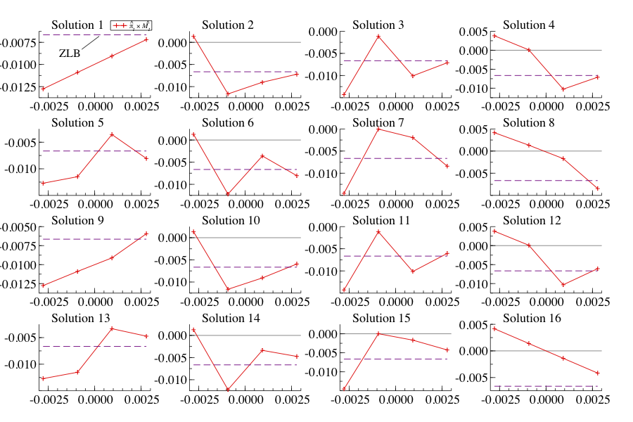
Figure 14: The equilibria of model $\hat{\pi}_{t|t+1}=max(-\mu,\psi\hat{\pi}_{t})+\hat{M}_{t+1|t}$, when $\mu=0.01$, $\psi=1.5$ and $\hat{M}_{t}$ follows a 4-state Markov Chain with mean 0, conditional st. dev. $\sigma=0.0007$, and autocorrelation $\rho=0.9$.

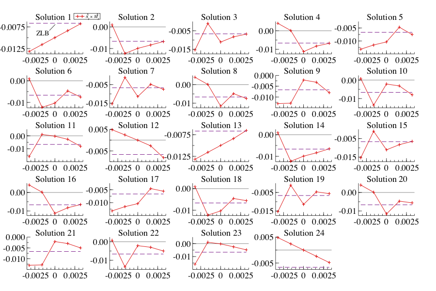
Figure 15: The equilibria of model $\hat{\pi}_{t|t+1}=max(-\mu,\psi\hat{\pi}_{t})+\hat{M}_{t+1|t}$, when $\mu=0.01$, $\psi=1.5$ and $\hat{M}_{t}$ follows a 5-state Markov Chain with mean 0, conditional st. dev. $\sigma=0.007$, and autocorrelation $\rho=0.9$.

A.8 A model with ZLB on inflation expectations

In this section we exemplify how the coherency of a model with a second inequality constraint can be analysed using the methodology of this paper. We consider Example ACS with an addition ZLB on inflation expectation, motivated by Gorodnichenko and Sergeyev (2021). The model is given by

$$\max\left\{\hat{\pi}_{t+1|t},0\right\}=\max\left\{-\mu,\psi\hat{\pi}_{t}\right\}+\hat{M}_{t+1|t}.$$ (A90)

Suppose $\hat{M}_{t}$ follows a $k$-state Markov chain, with states $m$ and transition probability kernel given by the $k\times k$ matrix $K$ with $K_{ij}=\Pr\left(\hat{M}_{t+1}=m_{j}|\hat{M}_{t}=m_{i}\right)$.

$$E_{t}\left(\hat{\pi}_{t+1}\right)=K\pi,\quad E_{t}\left(\hat{M}_{t+1}\right)=Km,$$

and so the equation to be solved, (A90), can be written as

$$\max\left(K\pi,0\right)=Km+\max\left(-\mu\iota_{k},\psi\pi\right).$$

This is a system of piecewise linear equations with two inequality constraints $K\pi\geq 0$ and $\pi\geq-\mu/\psi.$ This defines at most $4^{k}$ cones because some inequality combinations may be impossible. The following graph illustrates for the case $k=2$ where the first state is transitory and persists with probability $p$ and the second state is absorbing. The ZLB on the interest rate generates the inequalities we defined previously, i.e., $\pi_{t}>-\mu/\psi$ is a PIR and $\pi_{t}\leq-\mu$ is a ZIR. The ZLB on expectations is

$$E_{t}\left(\pi_{t+1}\right)\geq 0\Rightarrow\left\{\begin{array}[c]{ll}p\pi_{1}+\left(1-p\right)\pi_{2}\geq 0,&\text{if }\hat{M}_{t}\text{ transitory}\\ \pi_{2}\geq 0,&\text{if }\hat{M}_{t}\text{ absorbing.}\end{array}\right.$$

The possible regime configurations induced by combining the two inequalities are depicted in Figure 16. We see that these inequalities split $\Re^{2}$ into 10 cones. Let Z,P denote the interest rate regimes ZIR and PIR, respectively, and Z_e,P_e the expectations regime. So, (P,P;P_e,P_e) denotes positive interest rate and positive expectations in both states. The model can then be written in canonical form (5) with $\mathcal{A}_{J}$ for each cone defined as shown in Table 3.

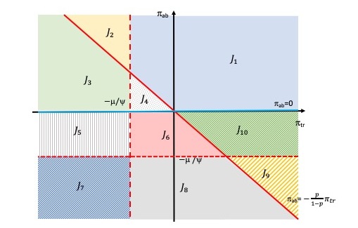
Figure 16: Combination of regimes in Example ACS with additional ZLB on inflation expectations. Dotted lines delineate interest rate regimes. Solid lines delineate expectations regimes in transitory (red) and absorbing (blue) states. Regimes are denoted by $J_{i}$.

Coefficient matrix ($2\times 2$)	Int. rate regime	Infl. exp. regime
$\mathcal{A}_{J_{1}}=K-\psi I$	P,P	Pe,Pe
$\mathcal{A}_{J_{2}}=K-\psi e_{2}e_{2}^{T}$	Z,P	Pe,Pe
$\mathcal{A}_{J_{3}}=e_{2}e_{2}^{T}K-\psi e_{2}e_{2}^{T}$	Z,P	Ze,Pe
$\mathcal{A}_{J_{4}}=e_{2}e_{2}^{T}K-\psi I$	P,P	Ze,Pe
$\mathcal{A}_{J_{5}}=-\psi e_{2}e_{2}^{T}$	Z,P	Ze,Ze
$\mathcal{A}_{J_{6}}=-\psi I$	P,P	Ze,Ze
$\mathcal{A}_{J_{7}}=0$	Z,Z	Ze,Ze
$\mathcal{A}_{J_{8}}=-\psi e_{1}e_{1}^{T}$	P,Z	Ze,Ze
$\mathcal{A}_{J_{9}}=e_{1}e_{1}^{T}K-\psi e_{1}e_{1}^{T}$	P,Z	Pe,Ze
$\mathcal{A}_{J_{10}}=e_{1}e_{1}^{T}K-\psi I$	P,P	Pe,Ze

Table 3: Coefficients of canonical representation (5) of Example ACS with an additional ZLB on inflation expectations.

We see by inspection that the CC condition in the GLM Theorem is violated, since some of the $\mathcal{A}_{J}$ are evidently singular. Even if we restrict attention to $\pi_{2}\geq 0,$ i.e., regimes $J_{1}$ to $J_{4}$, the determinants are (for $\psi>1$): $\det\mathcal{A}_{J_{1}}=\left(\psi-1\right)\left(\psi-p\right)>0$, $\det\mathcal{A}_{J_{2}}=p\left(1-\psi\right)<0$, $\det\mathcal{A}_{J_{3}}=0$ and $\det\mathcal{A}_{J_{4}}=\psi\left(\psi-1\right)>0$. So, this model is not generically coherent.

References

- Armenter (2018) Armenter, R., 2018. The perils of nominal targets. Rev. of Economic Studies 85, 50–86.
- Aruoba et al. (2021a) Aruoba, S.B., Cuba-Borda, P., Higa-Flores, K., Schorfheide, F., Villalvazo, S., 2021a. Piecewise-Linear Approximations and Filtering for DSGE Models with Occasionally Binding Constraints. Rev. of Economic Dynamics 41, 96–120.
- Aruoba et al. (2018) Aruoba, S.B., Cuba-Borda, P., Schorfheide, F., 2018. Macroeconomic dynamics near the zlb: A tale of two countries. The Rev. of Economic Studies 85, 87–118.
- Aruoba et al. (2021b) Aruoba, S.B., Mlikota, M., Schorfheide, F., Villalvazo, S., 2021b. SVARs with occasionally-binding constraints. Journal of Econometrics Forthcoming.
- Bilbiie (2018) Bilbiie, F.O., 2018. Neo-Fisherian Policies and Liquidity Traps. CEPR Discussion Papers 13334. C.E.P.R. Discussion Papers.
- Blanchard and Kahn (1980) Blanchard, O.J., Kahn, C.M., 1980. The solution of linear difference models under rational expectations. Econometrica 48, 1305–11.
- Boneva et al. (2016) Boneva, L.M., Braun, R.A., Waki, Y., 2016. Some unpleasant properties of loglinearized solutions when the nominal rate is zero. Journal of Monetary Economics 84, 216–232.
- Chen et al. (2012) Chen, H., Cúrdia, V., Ferrero, A., 2012. The macroeconomic effects of large-scale asset purchase programmes. The Economic Journal 122, F289–F315.
- Christiano et al. (2011) Christiano, L., Eichenbaum, M., Rebelo, S., 2011. When Is the Government Spending Multiplier Large? Journal of Political Economy 119, 78–121.
- Christiano et al. (2018) Christiano, L., Eichenbaum, M.S., Johannsen, B.K., 2018. Does the New Keynesian Model Have a Uniqueness Problem? Working Paper. National Bureau of Economic Research.
- Dubi (2009) Dubi, C., 2009. An algorithmic approach to simultaneous triangularization. Linear Algebra and its Applications 430, 2975–2981.
- Eggertsson (2011) Eggertsson, G.B., 2011. What Fiscal Policy is Effective at Zero Interest Rates?, in: NBER Macroeconomics Annual, Volume 25. National Bureau of Economic Research, pp. 59–112.
- Eggertsson et al. (2021) Eggertsson, G.B., Egiev, S.K., Lin, A., Platzer, J., Riva, L., 2021. A toolkit for solving models with a lower bound on interest rates of stochastic duration. Rev. of Economic Dynamics .
- Eggertsson and Singh (2019) Eggertsson, G.B., Singh, S.R., 2019. Log-linear approximation versus an exact solution at the ZLB in the New Keynesian model. J. of Economic Dynamics and Control 105, 21–43.
- Eggertsson and Woodford (2003) Eggertsson, G.B., Woodford, M., 2003. Zero bound on interest rates and optimal monetary policy. Brookings papers on economic activity 2003, 139–233.
- Fernández-Villaverde et al. (2015) Fernández-Villaverde, J., Gordon, G., Guerrón-Quintana, P., Rubio-Ramirez, J.F., 2015. Nonlinear adventures at the zero lower bound. J. of Economic Dynamics and Control 57.
- Fernández-Villaverde et al. (2016) Fernández-Villaverde, J., Rubio-Ramírez, J.F., Schorfheide, F., 2016. Solution and estimation methods for DSGE models, in: Handbook of Macroeconomics. Elsevier. volume 2.
- Gorodnichenko and Sergeyev (2021) Gorodnichenko, Y., Sergeyev, D., 2021. Zero lower bound on inflation expectations. Mimeo.
- Gourieroux et al. (1980) Gourieroux, C., Laffont, J., Monfort, A., 1980. Coherency conditions in simultaneous linear equation models with endogenous switching regimes. Econometrica , 675–695.
- Guerrieri and Iacoviello (2015) Guerrieri, L., Iacoviello, M., 2015. Occbin: A toolkit for solving dynamic models with occasionally binding constraints easily. Journal of Monetary Economics 70, 22–38.
- Gust et al. (2017) Gust, C., Herbst, E., López-Salido, D., Smith, M.E., 2017. The empirical implications of the interest-rate lower bound. American Economic Review 107, 1971–2006.
- Holden (2021) Holden, T.D., 2021. Existence and uniqueness of solutions to dynamic models with occasionally binding constraints. Rev. of Economics and Statistics Forthcoming.
- Ikeda et al. (2020) Ikeda, D., Li, S., Mavroeidis, S., Zanetti, F., 2020. Testing the effectiveness of unconventional monetary policy in Japan and the United States. arXiv preprint. arXiv:2012.15158.
- Kulish et al. (2017) Kulish, M., Morley, J., Robinson, T., 2017. Estimating DSGE models with zero interest rate policy. Journal of Monetary Economics 88, 35–49.
- Mavroeidis (2021) Mavroeidis, S., 2021. Identification at the Zero Lower Bound. Econometrica 89, 2855–2885.
- Mendes (2011) Mendes, R.R., 2011. Uncertainty and the Zero Lower Bound: A Theoretical Analysis. MPRA Paper 59218. University Library of Munich, Germany.
- Mertens and Ravn (2014) Mertens, K., Ravn, M.O., 2014. Fiscal policy in an expectations driven liquidity trap. Rev. of Economic Studies 81, 1637–1667.
- Nakata (2018) Nakata, T., 2018. Reputation and liquidity traps. Rev. of Economic Dynamics 28, 252–268.
- Nakata and Schmidt (2019) Nakata, T., Schmidt, S., 2019. Conservatism and liquidity traps. Journal of Monetary Economics 104, 37–47.
- Nakata and Schmidt (2020) Nakata, T., Schmidt, S., 2020. Expectations-driven liquidity traps: Implications for monetary and fiscal policy. Technical Report 15422. CEPR Discussion Papers.
- Richter and Throckmorton (2015) Richter, A.W., Throckmorton, N.A., 2015. The zero lower bound: frequency, duration, and numerical convergence. The B.E. Journal of Macroeconomics 15, 1–26.
- Rouwenhorst (1995) Rouwenhorst, G.K., 1995. Asset pricing implications of equilibrium business cycle models, in: Cooley, T.F. (Ed.), Frontiers of Business Cycle Research. Princeton University Press, Princeton, NJ, pp. 294–330.