Quantum Self-Consistent Ab-Initio Lattice Dynamics

Abstract

The Quantum Self-Consistent Ab-Initio Lattice Dynamics package (QSCAILD) is a python library that computes temperature-dependent effective 2nd and 3rd order interatomic force constants in crystals, including anharmonic effects. QSCAILD’s approach is based on the quantum statistics of a harmonic model. The program requires the forces acting on displaced atoms of a solid as an input, which can be obtained from an external code based on density functional theory, or any other calculator. This article describes QSCAILD’s implementation, clarifies its connections to other methods, and illustrates its use in the case of the SrTiO₃ cubic perovskite structure.

PROGRAM SUMMARY

Program Title: QSCAILD
Licensing provisions: GNU General Public License version 3.0
Programming language: Python
External routines/libraries: MPI, NumPy, SciPy, spglib, phonopy, sklearn
Nature of problem: Calculation of effective interatomic force constants at finite temperature
Solution method: Regression analysis of forces from density functional theory coupled with a harmonic model of the quantum canonical ensemble, performed in an iterative way to achieve self-consistency of the phonon spectrum

1 Introduction

Lattice anharmonicity is at the origin of basic phenomena in solid state physics, such as thermal expansion, displacive phase transitions or intrinsic thermal resistivity. In the quasi-harmonic approximation, the volume dependence of lattice vibrations is taken into account to model thermal expansion and as a consequence the phonon spectrum becomes temperature-dependent. However, the definition of phonons in an anharmonic potential as interacting quasiparticles with a temperature-dependent population also implies that even at constant volume their energy can depend on temperature. The last decade has seen a tremendous improvement in the quantitative description of such temperature-dependent phonon properties in solids based on Density Functional Theory. A precursor of current methods is the Self-Consistent Ab-Initio Lattice Dynamics (SCAILD) approach proposed by Souvatzis et al. in 2008 [1], which is based on a self-consistent calculation of phonon frequencies using a collection of supercells in which atoms were displaced according to the thermal mean square displacement in the classical limit. Subsequent developments are the Temperature Dependent Effective Potential (TDEP) method [2], based on fitting effective force constants to the results of ab initio molecular dynamics; and the Stochastic Self-Consistent Harmonic Approximation (SSCHA) [3], which aims at mimizing the free energy of the system within a harmonic density matrix ansatz. More recently, other methods and implementations have appeared (see for instance Refs. [4, 5, 6, 7, 8]), showing that the field is becoming broader and raising increasing interest. The approach that we describe in this paper was first implemented in 2016 [9] and has been refined and improved since then. A similar procedure is also described in Ref. [10]. It is directly related to the original SCAILD approach, the main difference being that it lifts the approximation to the statistics of atomic displacements made at the time. This is why we name it QSCAILD, for Quantum Self-Consistent Ab-Initio Lattice Dynamics. Below we describe the technical details of the implementation that we publicly release and show a selection of results obtained with the code.

2 Methodology

2.1 Basic principle

For $N$ ions with a harmonic Hamiltonian $\mathcal{H}$, let $\rho_{\mathcal{H}}\left(u\right)$ be the probability of finding the system in a configuration in which each ion $i$ is displaced in Cartesian direction $\alpha$ by $u_{i\alpha}$. This probability is proportional, up to a normalization factor, to $\exp\left(-\frac{1}{2}u^{T}\mathbf{\Sigma}^{-1}u\right)$, where $\Sigma\left(i\alpha,j\beta\right)$ is the quantum covariance for atoms $i,j$ and directions $\alpha,\beta$:[9]

$$\Sigma\left(i\alpha,j\beta\right)=\frac{\hbar}{2\sqrt{M_{i}M_{j}}}\sum_{m}\omega_{m}^{-1}\left(1+2n_{B}\left(\omega_{m};T\right)\right)\epsilon_{mi\alpha}\epsilon_{mj\beta}^{*}.$$

Here, $M_{i}$ is the $i$-th atomic mass, $\omega_{m}$ the phonon frequency of mode $m$ (comprising both wavevector and branch degrees of freedom), $\mathbf{\epsilon}_{m}$ the corresponding eigenvector and $n_{B}$ the Bose-Einstein distribution at temperature $T$. The method obtains a self-consistent set of interatomic force constants by the following iterative procedure:

• The matrix $\mathbf{\Sigma}$ is computed from the phonon frequencies and eigenvectors and used to generate a random set of atomic displacements $\left\{u_{i\alpha}^{(n)}\right\}$, with $i\alpha$ indexing each atom and direction in the supercell and $n$ denoting each given random configuration.

• The forces $\left\{f_{i\alpha}^{(n)}\right\}$ acting on each atom of the supercell generated by this set of displacements $\left\{u_{i\alpha}^{(n)}\right\}$ are used to fit the interatomic force constants of a model potential, using least-squares minimization.

This scheme is depicted in Fig. 1.

2.2 General workflow

The code is a Python library that can perform two tasks:

1. Starting from a set of interatomic force constants and a crystal structure, compute the thermal displacement matrix and generate a number of displaced configurations.

2. After the forces on the atoms in those configurations have been computed from DFT, collect the results and generate new effective force constants.

Between those two tasks, the user has to perform the DFT calculations using a workflow that is system-dependent and is thus not implemented by the code. This scheme has to be iterated until convergence is reached. The program keeps track of the successive iterations and can monitor the convergence. At present, the code is written to use input from the Vienna Ab-initio Simulation Package [11, 12] and Phonopy [13] force constants in full format, but it can be adapted to use another DFT code. It also uses a modified version of the thirdorder script [14]. The output is natively compatible with the ShengBTE [14] and almaBTE [15] software packages, so that thermal conductivity calculations including anharmonic renormalization of force constants can be performed in a straightforward way. This workflow is illustrated in Fig. 2.

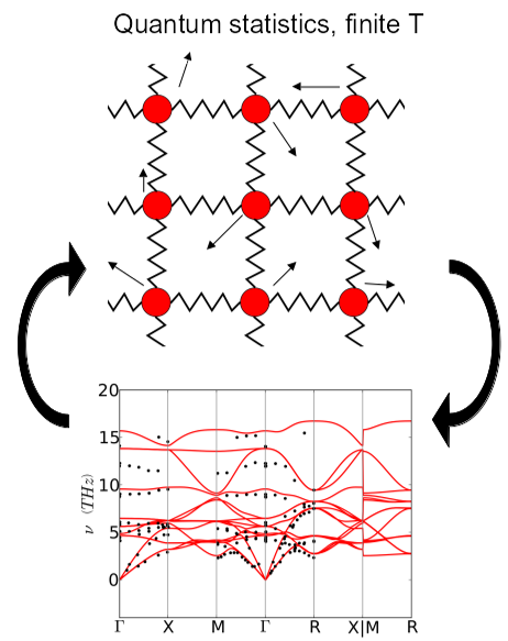
Figure 1: Simplified sketch of the QSCAILD method.

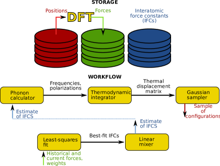
Figure 2: Workflow of the published implementation. This workflow can be wrapped in a driver that takes care of the optimization of lattice parameters and atomic positions.

2.3 Links to other methods

The link between the different methods cited in the introduction has not been discussed in depth in the literature, in particular regarding the connection between methods based on fitting forces from AIMD and methods based on minimizing the free energy within a harmonic Hilbert space. Here we show that the solution of the QSCAILD method is equivalent to the solution of the SSCHA, and thus holds the same properties, notably the minimization of the free energy. For each iteration, a sample of configurations is generated with density matrix $\rho_{\mathcal{H}}$. The forces are calculated and fitted to a harmonic force constant matrix $\Phi$ by least squares minimization of the quantity $S=\sum_{k,n}\left(s_{k}^{(n)}\right)^{2}$ over all sets of force constants compatible with the symmetries, with $s_{k}^{(n)}=f_{k}^{(n)}+\sum_{l}\Phi_{kl}u_{l}^{(n)}$, in which $n$ is a given configuration, and $k,l$ reduced indices for atom and Cartesian coordinates. The solution of the least squares problem satisfies $\frac{\partial S}{\partial\Phi_{ij}}=0$ for each $i,j$, so

$$2\sum_{k,n}s_{k}^{(n)}\frac{\partial s_{k}^{(n)}}{\partial\Phi_{ij}} = 0$$

$$\Rightarrow 2\sum_{k,n}s_{k}^{(n)}\frac{\partial\sum_{l}\Phi_{kl}u_{l}^{(n)}}{\partial\Phi_{ij}} = 0$$

$$\Rightarrow\sum_{n}s_{i}^{(n)}u_{j}^{(n)} = 0$$

$$\Rightarrow\sum_{n}\left(f_{i}^{(n)}-f_{\mathcal{\mathcal{H}}^{new}i}^{(n)}\right)u_{j}^{(n)} = 0.$$

Here, $\mathcal{H}^{new}$ is the Hamiltonian of the next iteration and $f_{\mathcal{H}^{new}k}=-\sum_{l}\Phi_{kl}u_{l}^{(n)}$ is the harmonic force. In the limit of an infinite number of configurations, we have for all $i,j$:

$$\int_{\mathbb{R}^{3N}}\left[\left(f_{i}-f_{\mathcal{H}^{new}i}\right)u_{j}\right]\rho_{\mathcal{H}}(u)du=0$$ (1)

When self-consistency is achieved, $\mathcal{H}^{new}=\mathcal{H}$, and the gradient of the free energy with respect to force constants coefficients in the sense of the SSCHA is zero, according to equation (22) of Ref. [16]. Together with equation (17) of Ref. [17], this shows that, at fixed point of the iteration (i.e., if and when convergence is achieved), the least-square fitting of forces is equivalent to performing the average of second derivatives of the potential. It is thus also equivalent to the approach described in Ref. [4]. A similar fit can be done using AIMD atomic configurations, in which case the harmonic density matrix is replaced by the MD density matrix, which does not contain zero point motion, but in turn is not limited to a harmonic form. In the case of a non-least-squares fit such as what is done with the LASSO algorithm, the minimization of the free energy is balanced with the requirement to obtain a sparse set of force constants [18]. Finally, we note that including the 3rd order force constants in the least-squares equation does not change the self-consistent solution: since $s_{k}^{(n)}=f_{k}^{(n)}+\sum_{l}\Phi_{kl}u_{l}^{(n)}+\sum_{lm}\Psi_{klm}u_{l}^{(n)}u_{m}^{(n)}$, we now have

$$\sum_{k,n}s_{k}^{(n)}\frac{\partial s_{k}^{(n)}}{\partial\Phi_{ij}}=\sum_{n}r_{i}^{(n)}u_{j}^{(n)} = 0$$

$$\Rightarrow\sum_{n}\left(f_{i}^{(n)}-f_{\mathcal{\mathcal{H}}^{new}i}^{(n)}\right)u_{j}^{(n)}+\sum_{lm,n}\Psi_{ilm}u_{l}^{(n)}u_{m}^{(n)}u_{j}^{(n)} = 0.$$

As we are working with a harmonic density matrix, for each $l,m,j$ we have

$$\int_{\mathbb{R}^{3N}}\left(u_{l}u_{m}u_{j}\right)\rho_{\mathcal{H}}(u)du=0$$ (2)

and the condition (1) is recovered. For the third order part, we expand:

$$\sum_{k,n}s_{k}^{(n)}\frac{\partial s_{k}^{(n)}}{\partial\Psi_{hij}}=\sum_{n}s_{h}^{(n)}u_{i}^{(n)}u_{j}^{(n)} = 0,$$

$$\sum\limits_{n}\left(f_{h}^{(n)}+\sum\limits_{lm}\Psi_{hlm}u_{l}^{(n)}u_{m}^{(n)}\right)u_{i}^{(n)}u_{j}^{(n)}$$

$$+\sum\limits_{l,n}\Phi_{hl}u_{l}^{(n)}u_{i}^{(n)}u_{j}^{(n)} = 0.$$

and, similarly, the second term on the left-hand side can be dropped in the limit of an infinite number of configurations, so the above equation becomes:

$$\int_{\mathbb{R}^{3N}}\left[\left(f_{h}-f_{\mathcal{H}^{new}h}^{(3rd)}\right)u_{i}u_{j}\right]\rho_{\mathcal{H}}(u)du=0$$ (3)

More generally, and for the same reasons related to the symmetry of the density matrix, an expansion of $f_{i}$ to all orders shows that, for fixed atomic positions, only even orders can renormalize the second-order part while odd orders renormalize the third order part of the effective Hamiltonian. When average atomic positions are not fixed by symmetry, their modification due to odd-order anharmonicity can have an impact on second order effective force constants. These new average positions can be computed by minimizing the average force, as described in Eq. (21) of Ref. [16]. A sample implementation is included in our code, although more complex workflows require the user to write a more complete driver. We also stress that here the density matrix is computed solely based on the second-order force constants to stay harmonic, although in principle this sampling could be improved.

In spite of equation (2) showing that including only second-order or both second and third-order terms in the fit should yield the same self-consistent effective harmonic force constants in the limit of an infinite number of configurations, in practice, and due to the necessarily finite number of samples, the inclusion of both second- and third-order terms improves the stability and speed of convergence of the algorithm. This result is not necessarily intuitive since the number of unknowns in the system is clearly increased. In general, we recommend a strongly overdetermined system with $5$ to $10$ times more forces than irreducible unknowns.

2.4 Potential and kinetic pressure

Below we show how we include the kinetic pressure term in our static simulation and the relation with the quasiharmonic approximation and with molecular dynamics.

A quantity that can be obtained from the DFT calculations is the stress tensor for each configuration, which contains only the derivative of the potential energy. We obtain the value of the diagonal elements $\{u\}$ in the case of a potential with 2nd and 3rd order terms, and we consider only the isotropic case for simplicity. When the volume changes from $V$ to $V+\Delta V$, the positions of the atoms in the cell change from $r_{i}=r_{i}^{eq}+u_{i}$ to $r_{i}\left(1+\frac{\Delta V}{3V}\right)$, such that the displacement with respect to equilibrium $u_{i}$ becomes $u_{i}+\Delta_{i}$ with $\Delta_{i}=r_{i}^{eq}\frac{\Delta V}{3V}+u_{i}\frac{\Delta V}{3V}$. We thus obtain, to the first order:

$$\Delta E_{p}=\frac{1}{2}\sum_{ij}\Phi_{ij}\left(\Delta_{i}u_{j}+u_{i}\Delta_{j}\right)+\frac{1}{6}\sum_{ijk}\Psi_{ijk}\left(\Delta_{i}u_{j}u_{k}+u_{i}\Delta_{j}u_{k}+u_{i}u_{j}\Delta_{k}\right)$$

$$\frac{\Delta E_{p}}{\Delta V}=\frac{1}{6V}\sum_{ij}\Phi_{ij}\left(r_{i}^{eq}u_{j}+u_{i}r_{j}^{eq}\right)+\frac{1}{6V}\left(2\sum_{ij}\Phi_{ij}u_{i}u_{j}\right)+\frac{1}{18V}\sum_{ijk}\Psi_{ijk}\left(r_{i}^{eq}u_{j}u_{k}+u_{i}r_{j}^{eq}u_{k}+u_{i}u_{j}r_{k}^{eq}\right)+\frac{1}{18V}\left(3\sum_{ijk}\Psi_{ijk}u_{i}u_{j}u_{k}\right).$$

Thus, the average of the diagonal elements of the stress tensor in the limit of infinite number of configurations is:

$$\int_{\mathbb{R}^{3N}}\frac{\Delta E_{p}}{\Delta V}\rho_{\mathcal{H}}(u)du=\frac{2}{3V}\int_{\mathbb{R}^{3N}}E_{p}\rho_{\mathcal{H}}(u)du+\frac{1}{6V}\int_{\mathbb{R}^{3N}}\sum_{ijk}\Psi_{ijk}r_{i}^{eq}u_{j}u_{k}\rho_{\mathcal{H}}(u)du$$ (4)

The second term on the right-hand side of equation 4 corresponds to the partial derivative of the free energy with respect to volume in the quasiharmonic approximation. The first term on the right hand side can be identified as a kinetic term using the quantum virial theorem, which is missing if only the mean stress tensor from DFT is taken, and reduces to the ideal gas expression in the limit of high temperature. This result can be generalized to the case of an anharmonic and anisotropic potential; marking the Cartesian directions $\alpha,\beta$ and the atomic index $i$, we write (as in Ref. [19]):

$$\sigma^{\alpha\beta}=\langle\sigma_{DFT}^{\alpha\beta}\rangle-\frac{1}{2V}\langle\sum_{i}u_{i}^{\alpha}f_{i}^{\beta}+u_{i}^{\beta}f_{i}^{\alpha}\rangle$$ (5)

The present version of the code only handles the diagonal elements of this stress tensor and thermal expansion is implemented for lattice vectors along the cartesian directions or cubic lattices. In practice, lattice parameters are iteratively modified until the calculated internal pressure equals the target pressure within a chosen tolerance (of the order of kbar).

2.5 Reweighting, mixing, and handling imaginary frequencies

As introduced for the SSCHA, one can reuse previously computed configurations with the help of a reweighting scheme. Each configuration $u$ drawn at cycle $B$ thus gets an associated weight $w$ that depends on the probability it would have to be drawn at the current cycle $C$ based on the current thermal displacement matrix $\Sigma_{C}$ and on the probability it had to be drawn at cycle $B$ based on the matrix that was used to draw it $\Sigma_{B}$:

$$w(u)=\frac{P_{\Sigma_{C}}(u)}{P_{\Sigma_{B}}(u)}$$ (6)

This reweighting scheme is implemented using the memory parameter, such that all configurations of cycles $\left\lfloor C\left(1-\text{memory}\right)\right\rfloor$ to $C$ are taken into account. We point out that this scheme is formally valid only at constant volume, such that in principle it should not be used along with thermal expansion updates – although in practice a short memory can still be used, at the risk of slightly inaccurate converged values.

How to handle the imaginary frequencies that might show up in the intermediate phonon spectra is a problem that dates back to the original implementation of the SCAILD method. At the time, it was chosen to switch them to the real axis with the same modulus [1]. This option is implemented in the code, but we also suggest another way to deal with those frequencies, which is to arbitrarily fix them to a finite real value. Those options are available using the imaginary_freq parameter.

Finally, it is usually better to use a strong mixing of the interatomic force constants to improve the stability of the self-consistency cycle, in particular close to phase transitions, since small stochastic deviations might lead to strong divergences. We point out that this treatment is only a way to attain the fixed point of the algorithm in certain cases. The obtained phonon spectrum has physical meaning only if it is fully self-consistent, otherwise the persistent presence of imaginary frequencies or the inability to find a fixed point only indicates a strong likelihood of mechanical instability.

2.6 Symmetries and acoustic sum rules

In a first step, irreducible elements of the 2nd and 3rd order interatomic force constants are identified using the crystal symmetries. Within the matrix space that can be constructed from those irreducible elements, we then identify eigenvectors that fulfill the acoustic sum rules using singular value decomposition, so that any force constants matrix generated by a combination of those eigenvectors respects the acoustic sum rule by construction. The operations that generate the full force constants matrix from each of those final irreducible elements are then stored in sparse format. They are characteristic of the crystal symmetry, so they can be used for compounds with the same structure but different chemistry. This part of the code does not run in parallel at present.

3 Example of SrTiO3

3.1 Convergence with respect to supercell size and wavevector grid

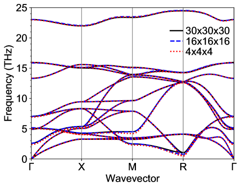
Figure 3: Band dispersion of cubic SrTiO₃ at 300 K obtained with different samplings of the Brillouin zone for phonon properties, computed in a 4x4x4 supercell with $\Gamma$-point sampling for the electrons and the PBEsol functional.

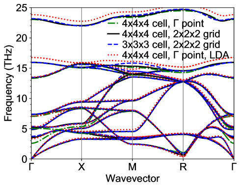
Figure 4: Band dispersion of cubic SrTiO₃ at 300 K obtained with different supercells and samplings of the Brillouin zone for the electronic properties, using the PBEsol and LDA functionals.

We computed the phonon dispersions and equilibrium lattice parameters at 300 K for different supercells and wavevector grid sizes, with convergence thresholds of $\pm 0.2\;\mathrm{GPa}$ for the internal pressure and $\pm 0.005\;\mathrm{eV/A^{2}}$ for the interatomic force constants. The obtained spectra are displayed in Figs. 3 and 4. The exchange-correlation functional was set to PBEsol except for a LDA calculation that is shown for the purposes of comparison. The non-analytical correction is applied based on ground-state Born charges and ion-clamped dielectric constant, but their temperature dependence could also be taken into account self-consistently [20]. One can see that the dispersion converges rather quickly within about 0.5 THz, and that the use of a different exchange-correlation functional appears to have a stronger impact. All in all, we typically observe a spread of the phonon frequencies between different calculations that translates into a spread of estimated transition temperatures of the order of 50 K to 100 K.

3.2 Temperature dependence and typical errors

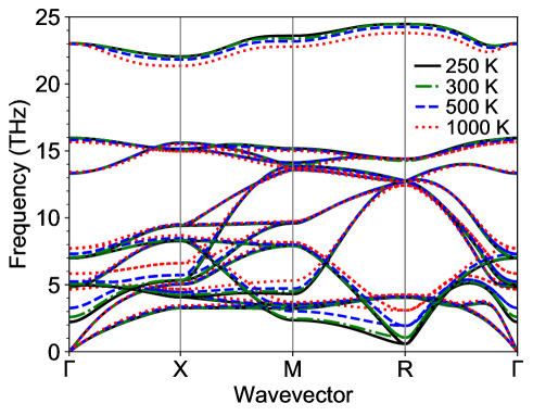
Figure 5: Temperature dependence of the phonon dispersion of cubic SrTiO₃ as obtained in the QSCAILD approach using the PBEsol exchange and correlation functional.

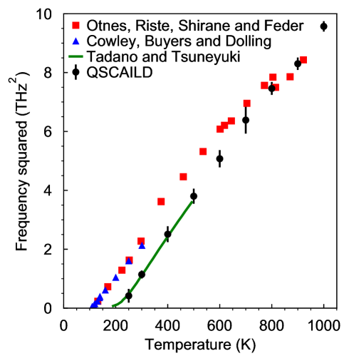
Figure 6: Temperature dependence of the square of the frequency of the soft mode at the R point of the Brillouin zone of cubic SrTiO₃. Experimental data from Refs. [21, 22] and computed data from Ref. [4] are superposed for comparison. Average values and standard deviations of the frequency squared were estimated based on 5 converged calculations at each temperature.

In the following, calculations were performed with a $4\times 4\times 4$ supercell and a $30\times 30\times 30$ wavevector grid. In Fig. 5 we display the phonon dispersion of SrTiO₃ at different temperatures obtained with the PBEsol exchange-correlation functional. Thermal expansion is taken into account, with a threshold for the average absolute pressure of 1 kbar. The temperature dependence of the soft mode displays the typical Curie-Weiss behavior (see Fig. 6), which allows us to extrapolate the transition temperature to about 200 K. We also note that it is in good agreement with the results obtained by Tadano and Tsuneyuki with the same functional [4]. The average frequency squared values and standard deviations were estimated by restarting new calculations from the converged solutions, to obtain a total of 5 solutions for each temperature. This also shows a typical spread of the phonon frequencies that can be interpreted in terms of temperature as a precision of the method of about 50 K to 100 K, for this particular system and convergence criteria.

4 Conclusion

We have described and implemented a method to obtain temperature-dependent, second and third order effective interatomic force constants. The method uses a regression analysis of forces from density functional theory, coupled with a harmonic model of the quantum canonical ensemble, and performed iteratively to achieve self-consistency of the phonon spectrum. We have discussed the relationship of this technique to other methods, showing that the resulting model minimizes the free energy of the system within the assumption of a harmonic density matrix, and proposed a way to include pressure from kinetic energy within this static scheme. Finally, we have computed the temperature-dependent force constants of SrTiO₃ with this method and found that it compares well with experimental results, and with previous calculations using a different technique. The program is open-source and available to the scientific community.

References

- [1] P. Souvatzis, O. Eriksson, M. I. Katsnelson, S. P. Rudin, Entropy driven stabilization of energetically unstable crystal structures explained from first principles theory, Phys. Rev. Lett. 100 (2008) 095901. doi:10.1103/PhysRevLett.100.095901.
- [2] O. Hellman, I. A. Abrikosov, S. I. Simak, Lattice dynamics of anharmonic solids from first principles, Phys. Rev. B 84 (2011) 180301. doi:10.1103/PhysRevB.84.180301.
- [3] I. Errea, M. Calandra, F. Mauri, First-principles theory of anharmonicity and the inverse isotope effect in superconducting palladium-hydride compounds, Phys. Rev. Lett. 111 (2013) 177002. doi:10.1103/PhysRevLett.111.177002.
- [4] T. Tadano, S. Tsuneyuki, Self-consistent phonon calculations of lattice dynamical properties in cubic SrTiO3 with first-principles anharmonic force constants, Phys. Rev. B 92 (2015) 054301. doi:10.1103/PhysRevB.92.054301.
- [5] Y. Xia, Revisiting lattice thermal transport in PbTe: The crucial role of quartic anharmonicity, Appl. Phys. Lett. 113 (7) (2018) 073901. doi:10.1063/1.5040887.
- [6] A. Carreras, A. Togo, I. Tanaka, DynaPhoPy: A code for extracting phonon quasiparticles from molecular dynamics simulations, Comp. Phys. Comm. 221 (2017) 221 – 234. doi:10.1016/j.cpc.2017.08.017.
- [7] N. K. Ravichandran, D. Broido, Unified first-principles theory of thermal properties of insulators, Phys. Rev. B 98 (2018) 085205. doi:10.1103/PhysRevB.98.085205.
- [8] F. Eriksson, E. Fransson, P. Erhart, The hiphive package for the extraction of high-order force constants by machine learning, Advanced Theory and Simulations 2 (5) (2019) 1800184. doi:10.1002/adts.201800184.
- [9] A. van Roekeghem, J. Carrete, N. Mingo, Anomalous thermal conductivity and suppression of negative thermal expansion in ScF3, Phys. Rev. B 94 (2016) 020303(R). doi:10.1103/PhysRevB.94.020303.
- [10] N. Shulumba, O. Hellman, A. J. Minnich, Intrinsic localized mode and low thermal conductivity of pbse, Phys. Rev. B 95 (2017) 014302. doi:10.1103/PhysRevB.95.014302.
- [11] G. Kresse, J. Furthmüller, Efficient iterative schemes for ab initio total-energy calculations using a plane-wave basis set, Phys. Rev. B 54 (1996) 11169–11186. doi:10.1103/PhysRevB.54.11169.
- [12] G. Kresse, D. Joubert, From ultrasoft pseudopotentials to the projector augmented-wave method, Phys. Rev. B 59 (1999) 1758–1775. doi:10.1103/PhysRevB.59.1758.
- [13] A. Togo, I. Tanaka, First principles phonon calculations in materials science, Scr. Mater. 108 (2015) 1–5. doi:10.1016/j.scriptamat.2015.07.021.
- [14] W. Li, J. Carrete, N. A. Katcho, N. Mingo, ShengBTE: a solver of the Boltzmann transport equation for phonons, Comp. Phys. Commun. 185 (2014) 1747–1758. doi:10.1016/j.cpc.2014.02.015.
- [15] J. Carrete, B. Vermeersch, A. Katre, A. van Roekeghem, T. Wang, G. K. Madsen, N. Mingo, almaBTE : A solver of the space–time dependent Boltzmann transport equation for phonons in structured materials, Comput. Phys. Commun. 220 (2017) 351 – 362. doi:10.1016/j.cpc.2017.06.023.
- [16] I. Errea, M. Calandra, F. Mauri, Anharmonic free energies and phonon dispersions from the stochastic self-consistent harmonic approximation: Application to platinum and palladium hydrides, Phys. Rev. B 89 (2014) 064302. doi:10.1103/PhysRevB.89.064302.
- [17] R. Bianco, I. Errea, L. Paulatto, M. Calandra, F. Mauri, Second-order structural phase transitions, free energy curvature, and temperature-dependent anharmonic phonons in the self-consistent harmonic approximation: Theory and stochastic implementation, Phys. Rev. B 96 (2017) 014111. doi:10.1103/PhysRevB.96.014111.
- [18] F. Zhou, W. Nielson, Y. Xia, V. Ozoliņš, Lattice anharmonicity and thermal conductivity from compressive sensing of first-principles calculations, Phys. Rev. Lett. 113 (2014) 185501. doi:10.1103/PhysRevLett.113.185501.
- [19] L. Monacelli, I. Errea, M. Calandra, F. Mauri, Pressure and stress tensor of complex anharmonic crystals within the stochastic self-consistent harmonic approximation, Phys. Rev. B 98 (2018) 024106. doi:10.1103/PhysRevB.98.024106.
- [20] A. van Roekeghem, J. Carrete, S. Curtarolo, N. Mingo, High-throughput study of the static dielectric constant at high temperatures in oxide and fluoride cubic perovskites, Phys. Rev. Materials 4 (2020) 113804. doi:10.1103/PhysRevMaterials.4.113804.
- [21] Relationship of normal modes of vibration of strontium titanate and its antiferroelectric phase transition at 110 K, Solid State Commun. 7 (1) (1969) 181 – 184. doi:10.1016/0038-1098(69)90720-0.
- [22] K. Otnes, T. Riste, G. Shirane, J. Feder, Temperature dependence of the soft mode in SrTiO3 above the 105 K transition, Solid State Commun. 9 (13) (1971) 1103 – 1106. doi:10.1016/0038-1098(71)90471-6.