Updated theoretical Period-Age and Period-Age-Color relations for Galactic Classical Cepheids: an application to the Gaia DR2 sample

Abstract

Updated evolutionary and pulsational model predictions are combined in order to interpret the properties of Galactic Classical Cepheids in the Gaia Data Release 2. In particular, the location of the instability strip boundaries and the analytical relations connecting pulsation periods to the intrinsic stellar parameters are combined with evolutionary tracks to derive reliable and accurate period-age, and the first theoretical period-age-color relations in the Gaia bands for a solar chemical abundance pattern ($Z$=$0.02$, $Y$=$0.28$). The adopted theoretical framework takes into account possible variations in the mass-luminosity relation for the core helium-burning stage as due to changes in the core convective overshooting and/or mass loss efficiency, as well as the impact on the instability strip boundaries due to different assumptions for superadiabatic convection efficiency. The inferred period-age and period-age-color relations are applied to a selected sample of both fundamental and first overtone Gaia Cepheids, and individual ages for the various adopted theoretical scenarios are derived. The retrieved age distributions confirm that a variation in the efficiency of superadiabatic convection in the pulsational model computations has a negligible effect, whereas a brighter Mass-Luminosity relation, as produced by mild overshooting, rotation or mass loss, implies significantly older age predictions. Moreover, older Cepheids are found at larger Galactocentric distances, while first overtone Cepheids are found to be systematically older than the fundamental ones. The comparison with independent age distribution analysis in literature supports the predictive capability of current theoretical framework.

1 Introduction

Classical Cepheids (CC) are the most important primary distance indicators in the Local Group and excellent tracers of relatively young (from a few tens to a few hundreds of Myr) stellar populations. Indeed, they are well known to obey period-luminosity (PL) and period-luminosity-color (PLC) relations which are traditionally used to calibrate secondary distance indicators and, in turn, to estimate the Hubble constant $H_{0}$ (see e.g. De Somma et al., 2020, hereafter DS20 and references therein) and (see e.g. Fiorentino et al., 2013; Marconi et al., 2005; Riess et al., 2011; Riess et al., 2019; Ripepi et al., 2019, and references therein). Stellar evolution models predict that CC correspond to central helium-burning of massive and intermediate-mass stars and obey a mass-luminosity (ML) relation that is also dependent on chemical composition, as well as on the efficiency of a number of non canonical physical processes such as rotation, core convective overshooting during the core hydrogen burning-phase, and mass loss efficiency during (mainly) the red giant branch stage (see, e.g. Catelan & Smith, 2015; Salaris & Cassisi, 2006, and references therein). The adopted ML relation affects the shape of light curves and radial velocity curves, the coefficients of PLC and period-Wesenheit (PW) relations and, hence, the Cepheid-based distance scale (see e.g. ; ; ; , and references therein).

By combining the existence of the ML relation for CC with the well known PL relation and the anti-correlation between mass and age, we can easily conclude that if CC obey a PL relation, they also have to obey a period-age (PA) relation. In particular, if the period increases, the luminosity and the mass also increase according to the PL and the ML relations, while the Cepheid age decreases. The existence of a PA relation has been extensively investigated in literature from both the observational and theoretical point of view (see e.g. Anderson et al., 2016; Efremov, 1978; Efremov & Elmegreen, 1998; Efremov, 2003; Grebel & Brandner, 1998; Inno et al., 2015; Magnier et al., 1997; Senchyna et al., 2015), with most of the applications related to cluster pulsators both in the Milky Way and in other Local Group galaxies, such as M31 and the Magellanic Clouds (MC), for which independent age estimates were available (see Bono et al., 2005; Efremov, 2003; Marconi et al., 2006, and references therein). However, Cepheid-based ages are more promising than age estimates based, for instance, on isochrone fitting to the cluster color-magnitude diagrams (CMD), because they only rely on the pulsation period, which can be measured with a high accuracy and is not affected by uncertainties in reddening, distance, and photometric calibration. In addition, the PA relation is also suitable to be applied to field pulsators and, hence, accurate relative age estimates, based on this method, can provide strong constraints on the existence of population age gradients in the various Galactic fields.

From the theoretical point of view, nonlinear convective pulsation models (Bono et al., 2005; Marconi et al., 2006) have been adopted to derive the first completely theoretical PA relations as a function of the assumed chemical composition. These authors also showed that, similarly to PL relations, the PA relation has an intrinsic dispersion that reflects the finite width of the instability strip (IS). Indeed, it is necessary to include a color term, featuring period-age-color (PAC) relations, in order to obtain more accurate individual ages (see e.g. Bono et al., 2005; Marconi et al., 2006; Ripepi et al., 2017, and references therein). More recently, on the basis of linear nonadiabatic convective Cepheid pulsation models, Anderson et al. (2016) derived theoretical PA relations as a function of both chemical composition and rotation, discussing how the change induced on the ML relation by variations in the rotation efficiency can significantly modify the predicted age at a fixed period. However, as stated above, PAC relations should be preferred to PA relations to infer individual Cepheid ages and, in turn, to constrain the star formation history of the Cepheid hosting stellar environments.

In this context, the large sample of Galactic CC (GCC) for which the Gaia spacecraft provided the parallaxes and proper motions with unprecedented accuracy, complemented with multiband photometry, offers a unique dataset to test the predictive capability of theoretical PA and PAC relations, such as the one based on the updated theoretical pulsational framework by DS20. In that paper, we presented a new extended set of nonlinear convective pulsation models for a solar chemical abundance ($Z$=$0.02$, $Y$=$0.28$) and a wide range of stellar masses and effective temperatures, covering the whole observed period range of GCC, and varying both the ML relation and the efficiency of superadiabatic convection. On this basis, the first predicted light curves, PLC and PW relations in the Gaia filters were derived and applied to a selected sample of Gaia Data Release 2 (DR2) GCC (see Ripepi et al., 2019, for the selection criteria).

By combining the theoretical predictions for Cepheid periods and colors based on these models with the stellar ages based on the updated stellar evolution predictions in the BaSTI database (Pietrinferni et al., 2004; Hidalgo et al., 2018), we can derive updated theoretical PA relations and the first PAC relations in the Gaia DR2 bands as a function of both the ML relation and the efficiency of superadiabatic convection. The extension of the pulsational model datebase to a wide range of metallicity and initial helium abundance, mandatory to study extragalactic Cepheids, as well as the implementation of updated prescriptions for the ML relation, will be the subject of an upcoming work (De Somma et al. 2020, in preparation).

Here we focus on the predictions for GCC as age indicators to complement the results presented in DS20 for Cepheids in the Gaia database. The organization of the paper is as follows. In Section 2, we deal with the theoretical scenario based on recent evolutionary and pulsation models. In Section 3, we discuss the derivation of updated PA and the first theoretical PAC relations in the Gaia filters, as a function of both the ML and the convective efficiency assumptions. In section 4, the obtained PAC relations are applied to a sample of GCC in the Gaia DR2 database to obtain individual ages and, in turn, the predicted age distribution. The conclusions and some future developments close the paper.

2 A theoretical scenario for Galactic Cepheids

2.1 The evolutionary framework

Our previous works on the theoretical PA relationship (see, Bono et al., 2005; Marconi et al., 2006) were based on the theoretical evolutionary framework developed by Pietrinferni et al. (2004), named the BaSTI library. However, since the first release of the BaSTI library, several improvements to the stellar physics inputs, some revisions of the solar metal distribution, and corresponding revisions of the solar metallicity (we refer to, e.g. Bergemann & Serenelli, 2014, and references therein for a detailed discussion on this issue) have become available. Therefore, the BaSTI library has been recently updated. This version is known as the BaSTI-IAC version, and takes into account all the presently available updates and improvements in the input physics. The new complete library for a scaled solar chemical mixture has been provided in Hidalgo et al. (2018), and we refer the interested reader to this reference for a detailed discussion on the physical framework adopted for the model computations. This notwithstanding, for the sake of completeness, it is important to briefly discuss here the main differences between the BaSTI-IAC models adopted in the present work and BaSTI predictions accounted for in Bono et al. (2005) and Marconi et al. (2006).

One of the main differences is associated with the use of different reference solar heavy element distributions. The previous BaSTI models were based on the solar mixture provided by Grevesse & Sauval (1998). The new ones take into account the recent, significant revisions of the solar metal distributions, and rely on measurements provided by Caffau et al. (2011), supplemented when necessary by the abundance estimates provided by Lodders (2010).

The treatment of overshooting beyond the Schwarzschild boundary of convective cores during the H-burning stage, is included as an instantaneous mixing between the formal convective border and layers at a distance $\lambda_{ov}H_{P}$ from this boundary – keeping the radiative temperature gradient in this overshooting region. $H_{P}$ is the pressure scale height at the Schwarzschild boundary, and $\lambda_{ov}$ is a free parameter that in the BaSTI-IAC model computations has been set equal to 0.2, decreasing to zero when the mass decreases below a certain value (typically, equal to $\sim 1.5M_{\odot}$). As the previous BaSTI library, the new BaSTI-IAC library provides two complete sets of evolutionary models alternatively accounting (non canonical models) or not accounting at all for core convective overshooting (canonical scenario).

The mass loss phenomenon is accounted for by using the Reimers (1975) formula, with the free parameter $\eta$ - present in this mass loss prescription - set equal to zero when neglecting mass loss, or to $\eta$=0.3 when mass loss is accounted for (we refer to Hidalgo et al., 2018, for the discussion about this choice).

The treatment of superadiabatic convection is based on the Böhm-Vitense (1958) flavor of the mixing length theory, using the formalism by Cox & Giuli (1968). The value of the mixing length free parameter, fixed via the standard solar model (SSM) calibration, to $\alpha_{ml}$ = 2.006, was kept constant for all stellar masses, initial chemical compositions and evolutionary phases.

As mentioned, the calibration of the SSM sets the value of $\alpha_{ml}$, and the initial solar He abundance $Y_{\odot}$ and metallicity $Z_{\odot}$: the BaSTI-IAC SSM – properly accounting for atomic diffusion of both He and metals – matches the empirical solar constraints with the following initial abundances $Z_{\odot}$=$0.01721$ and $Y_{\odot}$=$0.2695$.

For the present analysis, we selected the stellar models with the solar chemical composition and a mass range between $4M_{\odot}$ and $11M_{\odot}$, with a step of $0.5M_{\odot}$.

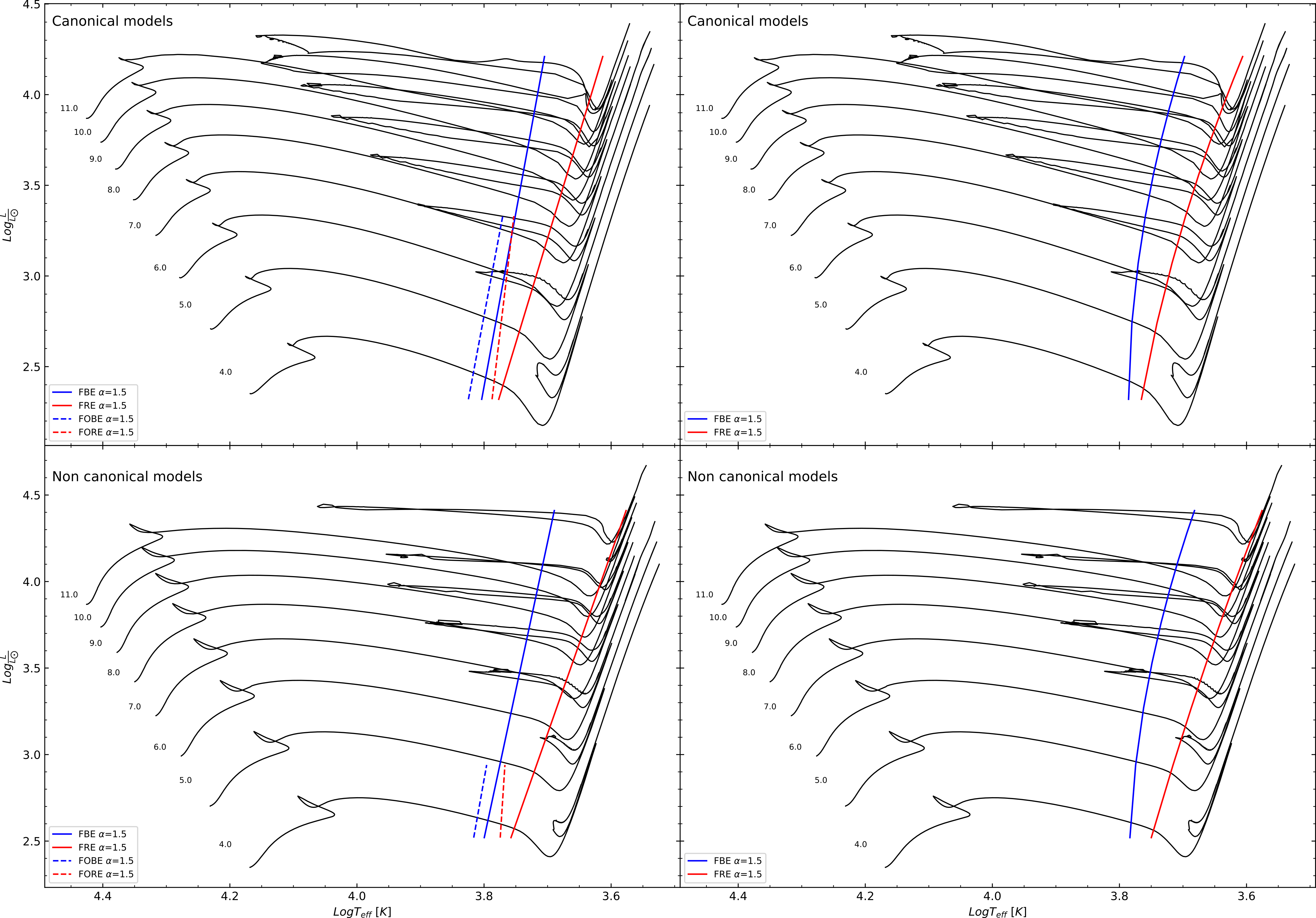
Figure 1: The location in the HR diagram of the selected massive and intermediate-mass stellar models for the adopted solar chemical composition, compared with the predicted linear IS boundaries (left panels) and quadratic IS boundaries (right panels) of radial F (solid line) and FO-mode pulsators (dashed line) as obtained for the canonical (top panels) and non canonical ML relation (bottom panels), assuming $\alpha_{ml}~{}$ = $1.5$. (see text for more details).

2.2 The pulsational framework

The pulsation models used in this work are included in the updated dataset of nonlinear and convective pulsation models computed for the chemical composition $Z$ = $0.02$, $Y$ = $0.28$, by DS20. By adopting the automated procedure described in that paper, we produced an extended dataset of fundamental (F) and first overtone (FO) models covering a wide range of input parameters.

For the first time a fine grid of pulsation models by simultaneously varying both the ML relation and the efficiency of superadiabatic convection was computed. More in detail, three ML relations were adopted: the canonical ML relation derived in Bono et al. (2000b) (named case A), obtained by neglecting mass loss, rotation and overshooting, a non canonical ML relation obtained by increasing the canonical luminosity level by $\Delta\log(L$/$L_{\odot})$=$~{}0.2$ (hereinafter case B) and, a still brighter ML relation obtained by increasing the canonical luminosity level by $\Delta\log(L$/$L_{\odot})$=$~{}0.4$ (named case C). The cases B and C for the ML relationship take into account the increase of the luminosity corresponding to the blue loop Cepheid stage, at a given stellar mass, induced by an increase of the mass size of the convective core during the central H-burning stage as due to non canonical processes such as convective overshooting and/or rotational induced mixing (we refer to Bono et al., 2005, for more details on this issue).

We note that, despite the improvements in the physical framework adopted for the BaSTI-IAC stellar model computation, the ML relationship predicted by the solar chemical composition, canonical (no overshooting) models is in quite good agreement with the the canonical ML relation adopted to build the Cepheid pulsation models (Bono et al., 2000b). At the same time, the increase of the brightness of the ML relationship by $\Delta\log(L$/$L_{\odot})$=$~{}0.2$ at a given stellar mass to simulate the effect of non canonical processes is consistent with the brightness increase of the ML relation predicted by the non canonical, BaSTI-IAC models with respect the corresponding canonical ones (we address the interested reader to Hidalgo et al., 2018, for a detailed comparison between the various model libraries). These considerations allow us to safely rely on the ML prescriptions based for developing the pulsational scenario adopted in the present work.

As for the superadiabatic convective efficiency, three values of the mixing length parameter were chosen; namely, $\alpha_{ml}$ =$1.5$ $\alpha_{ml}~{}$=$1.7$ and $\alpha_{ml}~{}$=$1.9$.

For the purpose of the current work, we considered only models with ML relations corresponding to cases A and B, and two assumptions on the efficiency of convection in the outer layers, namely $\alpha_{ml}~{}$=$1.5$ and $\alpha_{ml}~{}$=$1.7$. The reasons for not considering the brightest models and the highest $\alpha_{ml}$ value are related to the need for consistency with the adopted evolutionary scenario that do not predict overluminosities as high as +0.4 dex with respect to the canonical ML, and the small number of pulsating models obtained by DS20 for $\alpha_{ml}~{}$=$1.9$ (see DS20, for details).

The input parameters adopted for F and FO-mode models are listed in Tables 1 and 2 in DS20, respectively. For each assumed combination of mass, luminosity and $\alpha_{ml}$, the F and FO IS boundaries were derived by DS20. The linear fit of the inferred F and FO boundaries as a function of the luminosity level is reported in Tables 5 and 6 in DS20, while the quadratic fit coefficients are listed in current Table 1. In the case of the FO-mode, only the linear fit was taken into account due to the smaller number of pulsating models and the well known linear behaviour of the predicted edges (see e.g. Bono et al., 2000a, and references therein).

Figure 1 shows the location in the HR diagram of the linear (left panels) and quadratic (right panels) fits of the IS boundaries with respect the evolutionary tracks discussed in subsection 2.1. For clarity reason, only a subsample of stellar evolutionary tracks was plotted. Inspection of this figure suggests that stellar models with mass lower than about 5$M_{\odot}$, cross the predicted IS only once (first crossing), while evolving towards the Red Giant Branch. However, stars with masses higher than $\sim 5M_{\odot}$ show three crossings with the second and the third crossings corresponding to the blue-ward and red-ward evolution along the blue loop, respectively.

As expected on the basis of evolutionary considerations, the time spent during the first crossing is significantly shorter than the second and the third one. For example, in the case of a 6$M_{\odot}$ star the time spent inside the instability strip varies from $7.41\cdot 10^{3}yr$ for the ${\mathrm{1}^{th}}$ crossing to $3.73\cdot 10^{5}yr$ for the ${\mathrm{2}^{nd}}$ and $1.80\cdot 10^{5}yr$ for the ${\mathrm{3}^{rd}}$ one; while for a 11$M_{\odot}$ model the corresponding evolutionary lifetimes are $2.87\cdot 10^{3}$ $yr$ for the ${\mathrm{1}^{th}}$ crossing, and $3.16\cdot 10^{4}yr$ and $1.41\cdot 10^{4}yr$ for the ${\mathrm{2}^{nd}}$ and ${\mathrm{3}^{rd}}$ crossing, respectively.

For the reliability of evolutionary predictions about the blue loop morphology (and extension), it is worth mentioning that the physical reasons for the blue loops challenged for long time our understanding of stellar evolution, and it is still a difficult task to predict the response of an intermediate-mass stellar model, during this phase, to changes in the physical parameters and/or the physical assumptions adopted in the evolutionary computations. Indeed, both the morphology, and the actual occurrence of the blue loops have a highly non-linear dependence on the physical inputs and assumptions adopted in the stellar evolution models. Even minor changes, for example, in the chemical composition, initial mass, mixing process - such as convective core and envelope overshooting - efficiency can have huge impact on the blue loop properties (we refer to, e.g., Renzini et al., 1992; Salaris & Cassisi, 2006, and references therein for a detailed discussion on this topic).

Table 1: The coefficients of the quadratic relation $\log T_{eff}$ = a + b $\log$L/$L_{\odot}\,$+c ($\log$L/$L_{\odot}\,$)² for the boundaries of the F-mode IS, varying both the ML relation and the mixing length parameter.

$\alpha_{ml}$	ML	a	b	c	$\sigma_{a}$	$\sigma_{b}$	$\sigma_{c}$	$R^{2}$
FBE
1.5	A	3.667	0.104	-0.023	0.054	0.033	0.005	0.981
1.5	B	3.675	0.098	-0.022	0.053	0.031	0.004	0.988
1.7	A	3.708	0.092	-0.023	0.037	0.023	0.003	0.994
1.7	B	3.820	0.019	-0.012	0.069	0.040	0.005	0.986
FRE
1.5	A	3.788	0.030	-0.018	0.031	0.019	0.003	0.998
1.5	B	3.901	-0.042	-0.007	0.150	0.087	0.012	0.968
1.7	A	3.773	0.044	-0.018	0.050	0.031	0.005	0.993
1.7	B	3.645	0.121	-0.030	0.042	0.025	0.003	0.997

3 Tools for deriving Galactic Classical Cepheids ages

3.1 The theoretical Period-Age relation

In order to derive theoretical PA relations, we combined the evolutionary tracks with the predicted instability strips and pulsation periods inferred from the pulsation models computed in DS20.

At first, we adopted two different sub-samples: one including all the crossings and the other including only the second and third crossings. However, since we verified that the resulting PA relations are not significantly affected by the choice of specific sub-sample, in the following we only consider the relations obtained including all the crossings. Incidentally, we note that this choice is also consistent with the methodological approach adopted by Bono et al. (2005) and Marconi et al. (2006) to derive the PA relationship.

Adopting the period-luminosity-mass-temperature (PMLT) relation in the form $\log P$ = a + b$\log T_{eff}$ + c $\log$ $M$/$M_{\odot}\,$+ d $\log$L/$L_{\odot}\,$, derived by DS20, we were able to predict the period for each combination of mass, luminosity and effective temperature along the selected portions of the evolutionary tracks. By combining the period estimate with the age predicted by the evolutionary models, we directly derived the theoretical PA relations through a linear regression procedure. The coefficients obtained for each combination of ML and convective efficiency, assuming both linear and quadratic fits to the F boundaries, are reported in Tables 2 and 3, respectively. We notice that, due to the limited number of FO-mode models, in this case only the PA relations based on linear boundaries were obtained.

Figure 2 shows a comparison between the predicted PA relations for F pulsators with $\alpha_{ml}~{}$=$1.5$ and $\alpha_{ml}~{}$=$1.7$, in the case A ML relation and assuming both the quadratic (right panel) and the linear (left panel) boundary analytical relations.

The data shown in this figure reveal that the PA relation is largely unaffected by the exact value of the mixing length parameter adopted in the pulsational model computations; therefore, one can safely assume that the predicted Cepheid ages are barely affected by the lingering uncertainties in the adopted mixing length parameter.

Figure 3 shows the same kind of comparison but varying the ML relation at a fixed $\alpha_{ml}~{}$=$1.5$. In this case, we notice that brighter ML relations provide systematically older ages. This result is consistent with the theoretical prediction of a longer core hydrogen burning stage for stellar models accounting for core convective overshooting as the ones that have been combined with our case B pulsation models; an occurrence obviously due to the larger amount of fuel available during the central H-burning stage. In particular, the age difference between case B and A ranges from $\sim$ 36 % at $\log{P}$=$0.4$ to $\sim$ 60 % at $\log{P}$=$1.8$. We notice that the period range in these figures is the same as that estimated by DS20 (we refer to the quoted reference for more details) for cases A and B models. As the relations obtained assuming linear and quadratic F boundaries are found to be perfectly consistent within the errors, in the following we only rely on the relations obtained assuming linear boundaries.

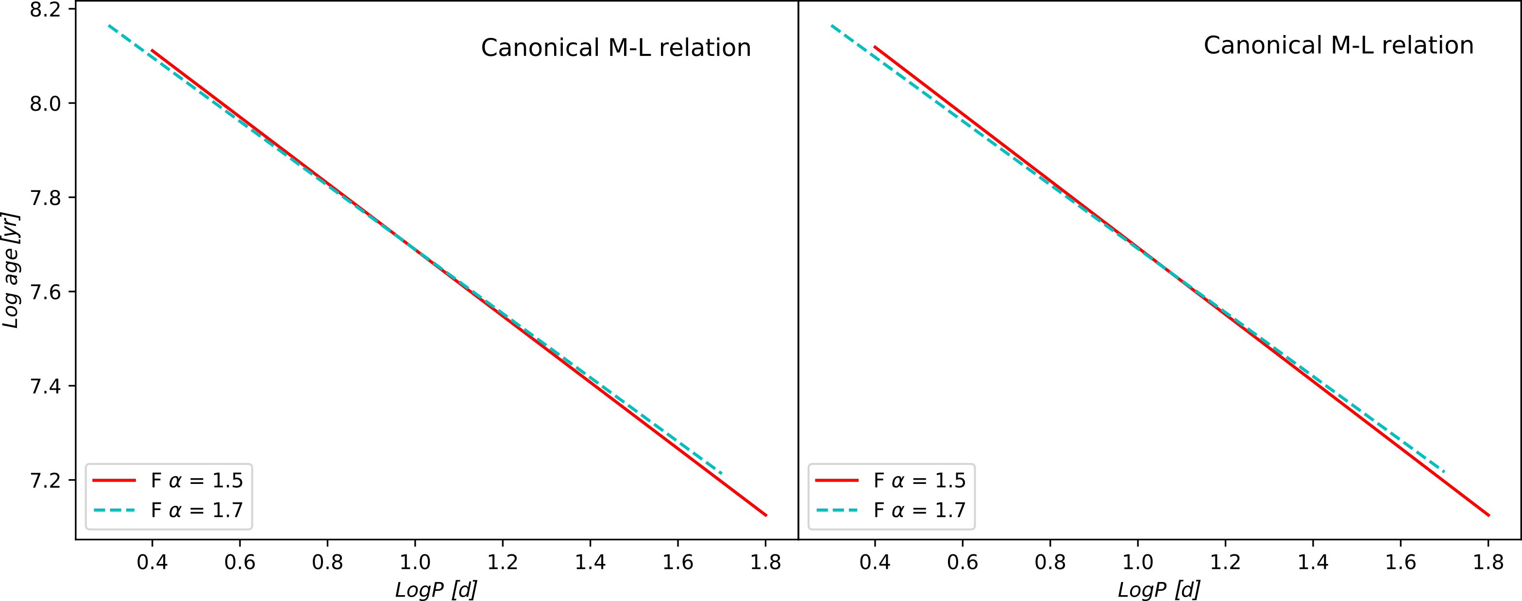
Figure 2: Canonical PA relations for the various assumptions about superadiabatic convective efficiency, assuming linear (left panel) and quadratic (right panel) analytical relations for the IS boundaries.

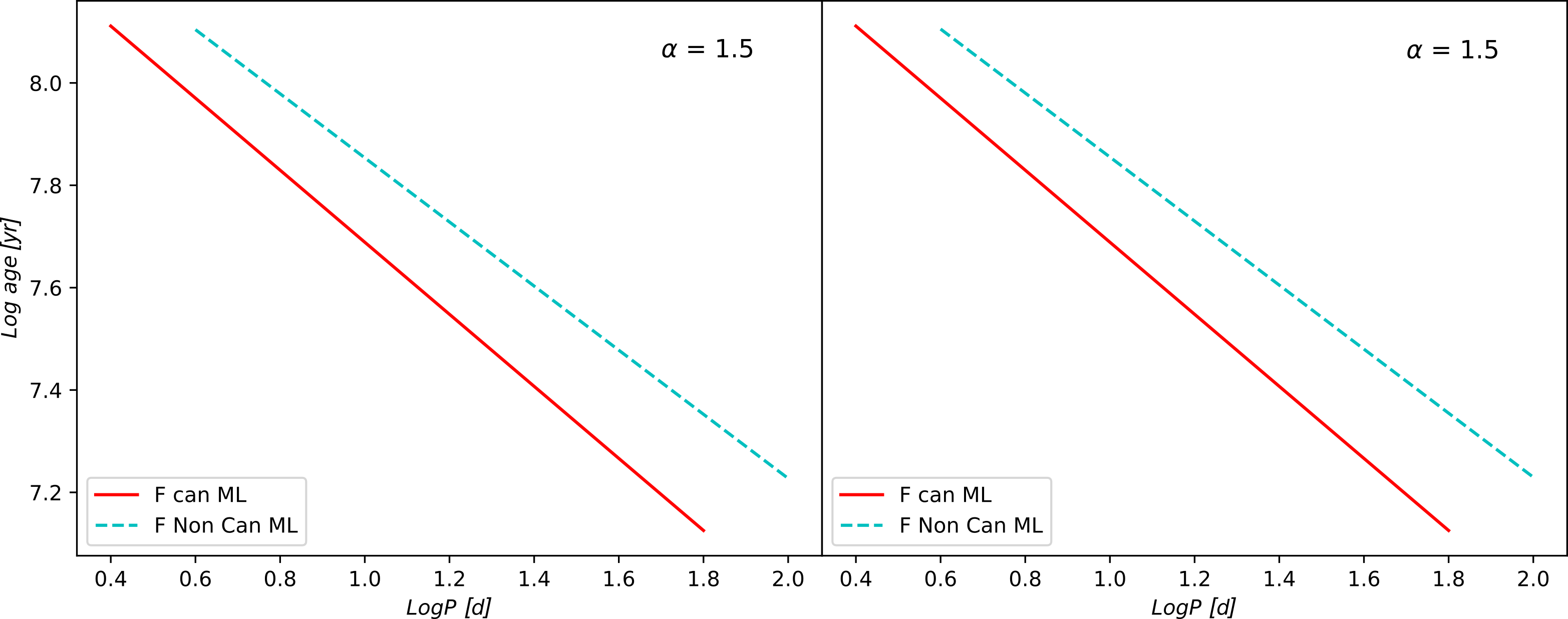
Figure 3: Fundamental PA relations at a fixed mixing length parameter $\alpha_{ml}~{}$=$1.5$ for the two assumed ML relations, assuming linear (left panel) and quadratic (right panel) IS boundary analytical relations.

Table 2: The coefficients of the F and FO PA relations in the form $\log t$ = $a$ + $b\log P$, assuming linear IS boundaries and adopting both case A and B ML relations and $\alpha_{ml}~{}$=$1.5$ and $\alpha_{ml}~{}$=$1.7$. The last two columns represent the R-squared ($R^{2}$) and the root-mean-square deviation ($\sigma$) coefficients.

Fundamental mode
$\alpha_{ml}$	ML	a	b	$\sigma_{a}$	$\sigma_{b}$	$R^{2}$	$\sigma$
1.5	A	8.393	-0.704	0.008	0.009	0.916	0.084
1.7	A	8.369	-0.680	0.015	0.017	0.908	0.080
1.5	B	8.480	-0.626	0.010	0.009	0.866	0.080
1.7	B	8.460	-0.618	0.013	0.010	0.852	0.090
First overtone mode
1.5	A	8.120	-0.396	0.020	0.057	0.506	0.052

Table 3: The coefficients of the F-mode PA relation $\log t$ = $a$ +$b\log P$, assuming quadratic IS boundaries and adopting both case A and B ML relations and $\alpha_{ml}~{}$=$1.5$ and $\alpha_{ml}~{}$=$1.7$. The last two columns represent the R-squared ($R^{2}$) and the root-mean-square deviation ($\sigma$) coefficients.

Fundamental mode
$\alpha_{ml}$	ML	a	b	$\sigma_{a}$	$\sigma_{b}$	$R^{2}$	$\sigma$
1.5	A	8.396	-0.708	0.007	0.009	0.910	0.083
1.7	A	8.362	-0.676	0.014	0.017	0.898	0.084
1.5	B	8.511	-0.660	0.010	0.009	0.856	0.090
1.7	B	8.477	-0.639	0.013	0.010	0.847	0.099

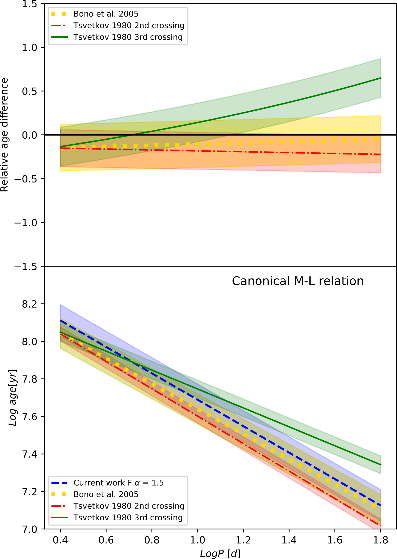
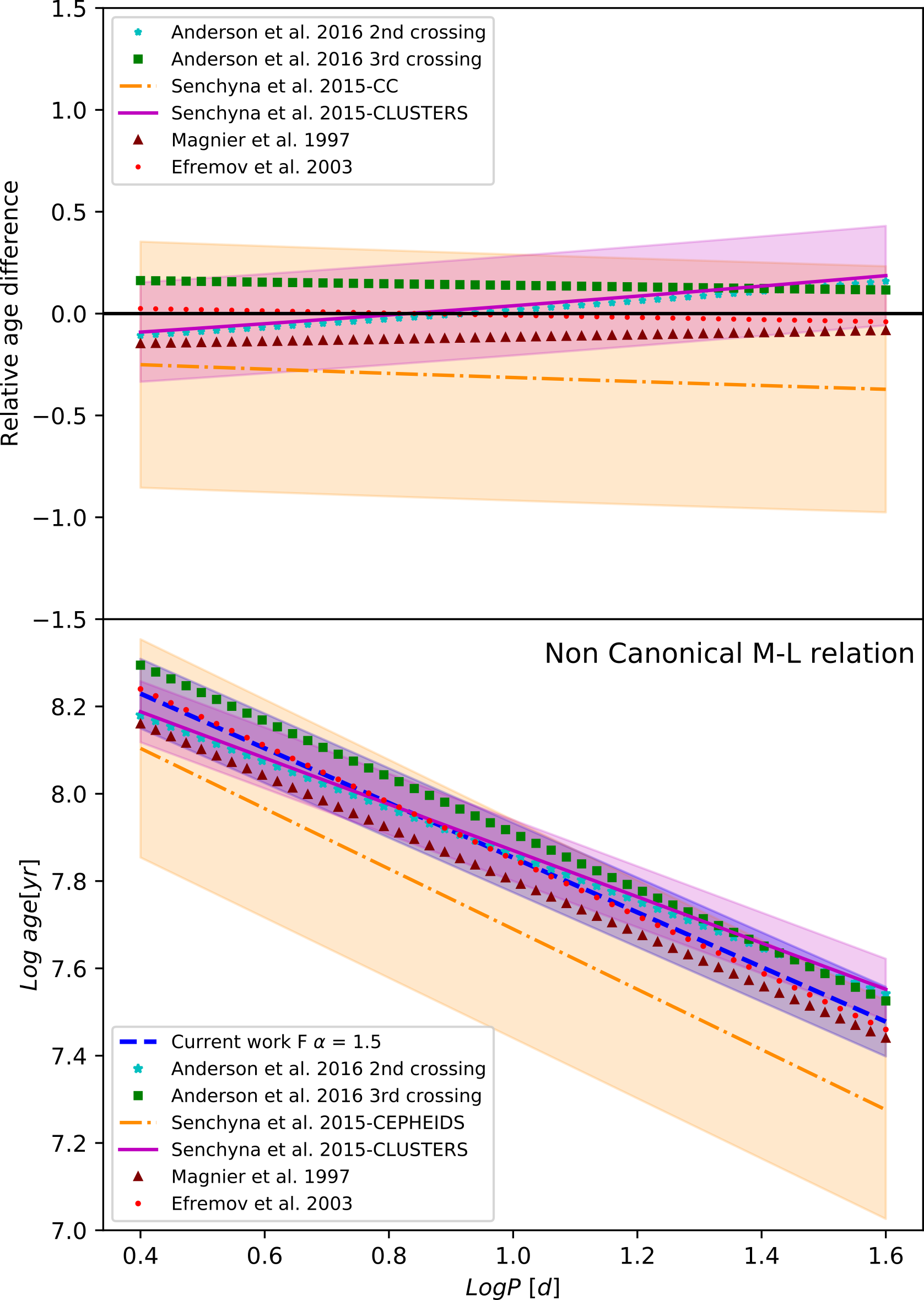
Figure 4: Bottom panels: comparison between present F-mode PA relations (dashed blue line), as obtained by varying the adopted ML relation (see labels) but at a fixed value for the mixing length ($\alpha_{ml}$), with similar predictions from the literature: the dashed red line and dash-dotted green line show the PA relations by Tsvetkov (1980), for the second and third crossings, respectively; the dotted yellow line shows the PA relation obtained by Bono et al. (2005); the relations marked with stars and squares represent the PA relations by Anderson et al. (2016), for the second and third crossings, respectively; the dash-dotted orange line refers to the PA relation by Senchyna et al. (2015) for M31 CC ; the solid magenta line is the PA relation by Senchyna et al. (2015) for M31 clusters; filled circles and triangles correspond to the PA relations by Efremov (2003) and Magnier et al. (1997), respectively. The colored shaded areas represent the $1\sigma$ errors on these relationships as provided by the authors. Upper panels: the relative age difference between the age predictions obtained by present PA relations for the canonical case (left panel) and the non canonical one (right panel) and those obtained with the mentioned PA relationships taken from the literature.

3.1.1 Comparison with the literature

In Figure 4 we compare our theoretical PA relations (dashed blue line) obtained for case A (left panels) and B ML (right panels)- by assuming in both cases $\alpha_{ml}~{}$=$1.5$, with other theoretical relations available in the literature. We selected a common period range for both case A (from $\log P~{}$=$~{}0.4$ to $\log P~{}$=$~{}1.8$) and B (from $\log P~{}$=$~{}0.4$ to $\log P~{}$=$~{}1.6$).

For the canonical case (left panels), we compare our case A relations with: i) the theoretical PA relation published by Bono et al. (2005) (dotted yellow line) and ii) the semi-empirical PA relations derived by Tsvetkov (1980) for the second (dashed red line) and third crossings (dash-dotted green line), respectively. For the non canonical case (right panels), we compare our case B relations with: i) the theoretical PA relations derived by Anderson et al. (2016) assuming a mild rotation efficiency, for the second (cyan star marker) and third crossings (green square marker), respectively; ii) the semi-empirical PA relations by Senchyna et al. (2015) based both on M31 Cepheids (dash-dotted orange line) and on M31 cluster isochrone fitting (solid magenta line); iii) the semi-empirical relation provided by Magnier et al. (1997) (brown triangle marker) and iv) the empirical relationship by Efremov (2003) (red dot marker).

Figure 5 shows the same kind of comparison but for case A FO-mode models with $\alpha_{ml}~{}$=$1.5$ and the FO relation by Bono et al. (2005).

The coefficients of the various PA relations used for the comparison are summarized in Table 4.

Inspection of the bottom panels of Figures 4 and 5 suggests a very good agreement, within the errors, between our canonical PA relations and the one previously derived by Bono et al. (2005) on the basis of a less extended and updated set of models and a slightly different ML relation. No error estimate was provided by Anderson et al. (2016), Efremov (2003) and Magnier et al. (1997) but we found a good agreement between their (all non canonical) relations and our case B.

In order to better quantify the level of agreement among the various PA relationships, the two upper panels in Figure 4 show the relative age difference between the relations obtained in the present work and the ones selected from the literature for both the canonical and non canonical ML cases. For the canonical case, present PA relation predicts ages systematically larger than the other relations with a maximum difference of the order of $\sim 15-20$%. The smallest difference – well within the associated intrinsic dispersions – is found when considering the PA relation provided by Bono et al. (2005), while the maximum discrepancy is obtained when comparing the present result with the relation obtained by Tsvetkov (1980) for the third crossing. In this case the difference can also reach a value as large as $\sim 50$% and it can be likely related to the difference in luminosity between the second and the third crossings in spite of the quite similar evolutionary times.

For the non canonical case, the relative age differences are within $\sim 15-20$%, apart from the case of the PA relation, based on Cepheids in M31, provided by Senchyna et al. (2015), that predicts ages about 25% smaller than those provided by our relation. However, we wish to emphasize the large uncertainty associated to the Senchyna et al. (2015) Cepheid-based PA relationship. For the case of FO PA, the agreement is remarkably good: there is a difference of about 5% between present predictions and those obtained by using the Bono et al. (2005) relation, but again well within the errors.

The general good agreement among the various PA relations based on similar ML relations, as well as the age difference obtained when comparing the results based on canonical and non canonical stellar models support the idea that different assumptions on non canonical physical processes, e.g., moderate rotation as in Anderson et al. (2016), and mild overshooting as in the other semi-empirical relations, have the same effect of producing a brighter luminosity at a fixed mass, and in turn, an older age at a fixed period.

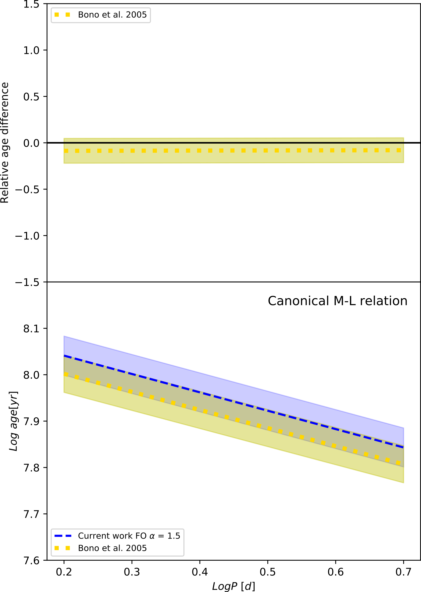
Figure 5: Bottom panel: comparison between present FO-mode PA relation (dashed blue line) obtained for ML case A and $\alpha_{ml}~{}$=$1.5$, with the theoretical FO-mode GCC PA relation obtained by Bono et al. (2005) (dotted yellow line). Upper panel: the relative difference between the age estimates provided by these PA relations.

Table 4: The PA relations $\log t$ = $a$ +$b\log P$ derived by various authors for different CC samples. $\sigma$ is the predicted root-mean-square deviation coefficient.

authors	source	a	b	$\sigma$
Anderson et al. (2016)	F GCC 2nd crossing	8.393	- 0.532
Anderson et al. (2016)	F GCC 3rd crossing	8.551	-0.641
Bono et al. (2005)	F GCC	8.31	-0.67	0.08
Bono et al. (2005)	FO GCC	8.08	-0.39	0.04
Efremov (2003)	LMC bar CC	8.50	-0.65
Magnier et al. (1997)	M31 CC	8.4	-0.6
Senchyna et al. (2015)	M31 CLUSTERS	8.40	-0.53	0.07
Senchyna et al. (2015)	M31 CC	8.38	-0.69	0.25
Tsvetkov (1980)	F GCC 2nd crossing	8.332	-0.731	0.037
Tsvetkov (1980)	F GCC 3rd crossing	8.250	-0.504	0.047

3.2 The theoretical Period-Age-Color relation in the Gaia filters

PA relations have the advantage to allow a direct evaluation of CC ages when only the pulsation periods are known, however they suffer from the limitation related to the finite color width of the IS, that causes - mostly in the optical photometric passbands - an inherent dispersion of PL relations. This occurrence implies that PA relations are also affected by an intrinsic scatter with a range of colors and periods for each fixed age; an effect than can be removed if a color term is included in the linear regression procedure.

As the main objective of the present work was to derive the individual ages of GCC with Gaia DR2 parallaxes, we used the Gaia band model light curves derived in DS20 and the resulting mean magnitudes $<G_{BP}>$ and $<G_{RP}>$, to compute the first PAC relations in the Gaia filters. Table 5 lists the coefficients of the derived PAC relations, for the F and FO-mode models and the discussed assumptions concerning ML and $\alpha_{ml}$.

In Figure 6, we compare the projections onto a plane of the PAC relations varying the assumptions on $\alpha_{ml}$ and the ML relations. As already found for the PA relations, a change in the super adiabatic convection efficiency does not affect the ages predicted from the new derived theoretical PAC relations. As a consequence, in the following we only adopt the PAC relation obtained for $\alpha_{ml}~{}$=$1.5$.

Table 5: The coefficients of the PAC relation: $\log t$ = $a$ + $b\log P$ + $c$ ($<G_{BP}>$ - $<G_{RP}>$), for F and FO pulsators, by varying both the ML relation and mixing length value.

Fundamental mode
$\alpha_{ml}$	ML	a	b	c	$\sigma_{a}$	$\sigma_{b}$	$\sigma_{c}$	$R^{2}$	$\sigma$
1.5	A	8.303	-0.751	0.121	0.045	0.025	0.060	0.916	0.083
1.7	A	8.346	-0.720	0.077	0.109	0.062	0.156	0.934	0.046
1.5	B	8.275	-0.734	0.278	0.029	0.017	0.037	0.876	0.077
1.7	B	8.453	-0.624	0.012	0.030	0.026	0.047	0.852	0.090
First overtone mode
1.5	A	7.961	-0.508	0.255	0.137	0.064	0.204	0.603	0.046

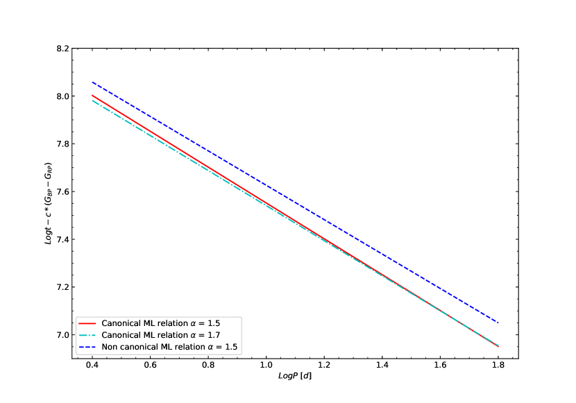
Figure 6: Projection onto a plane of the new Gaia band PAC relation (red solid line) for F-mode models as obtained by adopting case A ML and $\alpha_{ml}~{}$=$1.5$; for comparison the same relation as obtained by varying the super adiabatic convective efficiency (dash-dotted cyan line) or the ML relation (dashed blue line) is also shown.

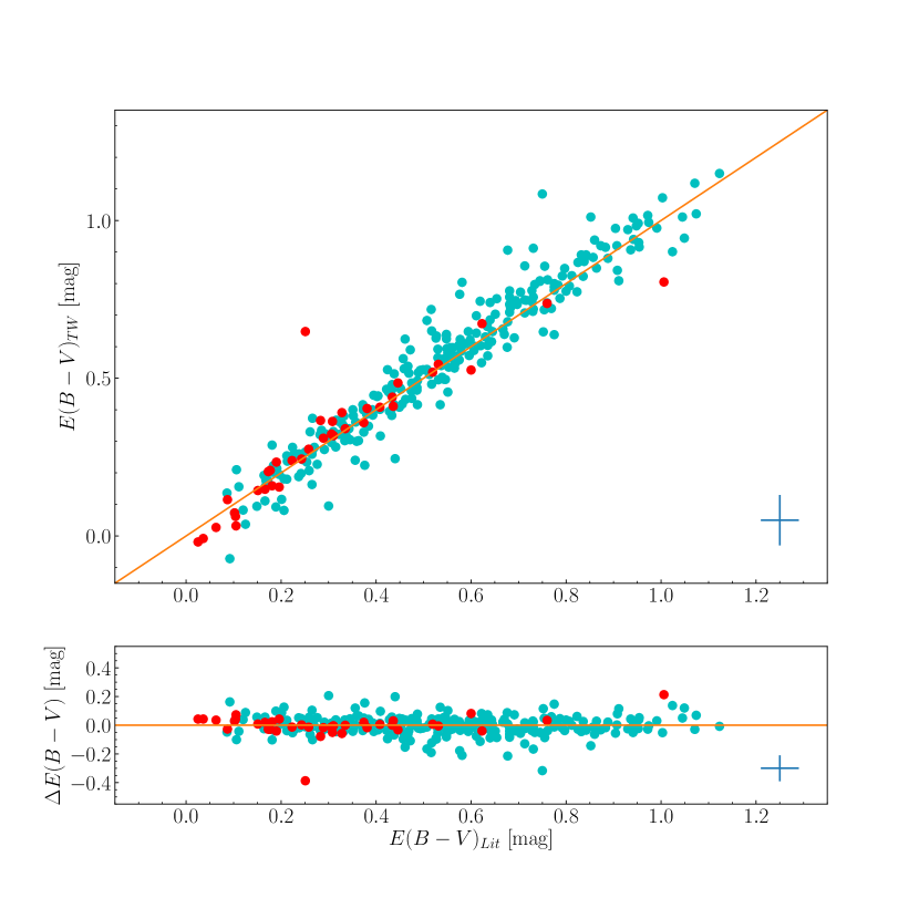
Figure 7: Comparison between the reddening values estimated from the period-$(V-I)_{0}$ relation E(B-V)_TW and the literature E(B-V)_Lit for a sample of 320 GCC (see text for more details). Top panel shows the 1:1 diagram; whilst bottom panel displays the difference between the two reddening estimates. In both panels, green and red filled circles represent F and FO pulsators, respectively.

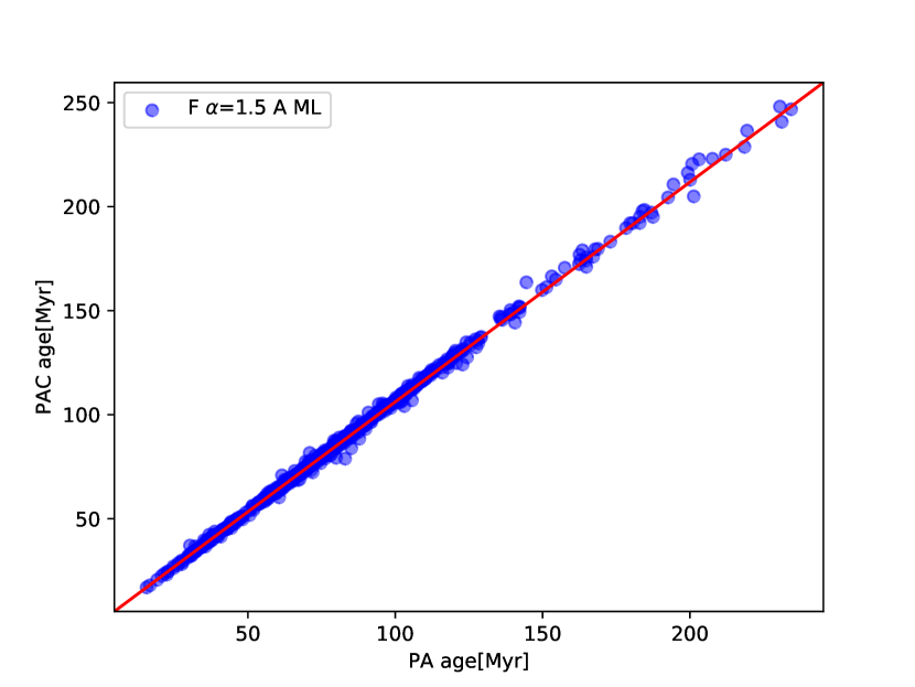
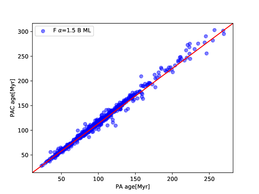
Figure 8: Comparison between the age estimates obtained by applying the PA and the PAC relations, for the two selected ML cases, (case A in the left panel and case B in the right panel) to the selected sub-sample of F-mode GCC. In both panels, the solid line represents the 1:1 line.

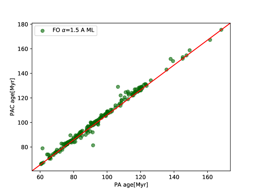
Figure 9: Comparison between the individual ages obtained by applying the PA and the PAC relations to the selected sub-sample of FO-mode GCC. The solid line represents the 1:1 line.

4 Individual ages of Gaia DR2 Galactic Classical Cepheids

In this section we apply the theoretical PA and Gaia-band PAC relations derived above to a sample of GCC published in the Gaia DR2 (Gaia Collaboration et al., 2018) and reclassified by Ripepi et al. (2019).

The selected sample consists of 568 F-mode and 198 FO-mode pulsators. Using the period and color values reported by Ripepi et al. (2019) and the PA and PAC relations, we derived the individual ages for each adopted assumption concerning the ML relation.

Before applying the PAC relation, it is mandatory to obtain dereddened ($G_{BP}-G_{RP}$) colors for the selected GCC sample. For this purpose, for 320 objects in common with our sample we adopted the E(B-V) estimates available in the compilation by Groenewegen (2018); for all other stars the CC period-(V-I)₀ color relation obtained by Ripepi et al. (in preparation) was used to derive the intrinsic unreddened color.

The (V-I) color estimate - averaged over the pulsation cycle - was obtained for 89 objects from the catalog of the OGLE Galactic Disk survey (Udalski et al., 2018); while for all other stars the averaged Gaia DR2 ($G_{BP}-G_{RP}$) color was transformed into the corresponding (V-I) one by using a conversion formula - suitable for the color range spanned by GCC - derived by Ripepi et al. (in preparation). These E(V-I) values were previously converted into E(B-V) by adopting the relation E(B-V)=1.283$\cdot$E(V-I) (Tammann et al., 2003), and lately into E($G_{BP}-G_{RP}$) by means of Eq. 9-10 in Ripepi et al. (2019). The average errors on the E(B-V) estimates are $\sim$0.08 mag and $\sim$ 0.11 mag, for the (V-I) color estimated from the OGLE survey and the Gaia magnitude conversion, respectively.

It is worth checking the level of consistency between the reddening estimates obtained by using the PC relation with those retrieved from the literature for the CC in the compilation of Groenewegen (2018); figure 7 shows a comparison between the E(B-V) values obtained with the two methods for both F and FO pulsators. The lack of any systematic trend in both the 1:1 (top panel) and the residuals (bottom panel) diagrams, supports the reliability of the approach used for estimating the extinction from the PC relation (Ripepi et al., in preparation).

We note that the reddening uncertainty affects the age measurements with an uncertainty of $\Delta(logt)\sim$0.009 dex and $\Delta(logt)\sim$ 0.022 dex for F-mode pulsators in cases A and B, respectively. For FO-mode GCC the uncertainty is $\Delta(logt)\sim$0.020 dex. As a consequence, the typical uncertainty on the GCC ages obtained from the PAC relationship, associated with the error on the reddening estimate, is of the order of 1-2%.

The GCC sample age estimates obtained by using the PA and PAC relationships are listed in Table 6 to 8.

In order to assess the accuracy of our age estimates, in Figures 8 and 9, we compare the individual age estimates obtained by applying the PA and the PAC relationships derived in the previous section, for the selected F and FO-mode GCC, respectively. In Figure 8, the two panels refer to case A (left) and B (right). It is worth noting that a good agreement does exist between the age measurements on the whole spanned age range obtained using the two relationships, as proven by the distribution of points with respect to the 1:1 line.

The histogram of the retrieved age distribution based on the application of the PAC relation, is shown in Figure 10, for both F (left panel) and FO (right panel) pulsators. Inspection of this figure confirms that the predicted ages depend on the assumed ML relation. Thus, providing systematically older ages for brighter ML relations, in agreement with independent evaluations in the literature (Anderson et al., 2016; Bono et al., 2005; Senchyna et al., 2015). For F-mode GCC, the left panel of Figure 10 suggests that the age distribution peaks around $\sim 90$ Myr in the assumption of a canonical ML relation (case A) and gets older by about $\sim 35$ Myr in the non-canonical assumption (case B). In the case of FO GCC (right panel of Figure 10), the inferred age distribution is - as expected - concentrated towards older ages with a peak between $(80-85)$ Myr.

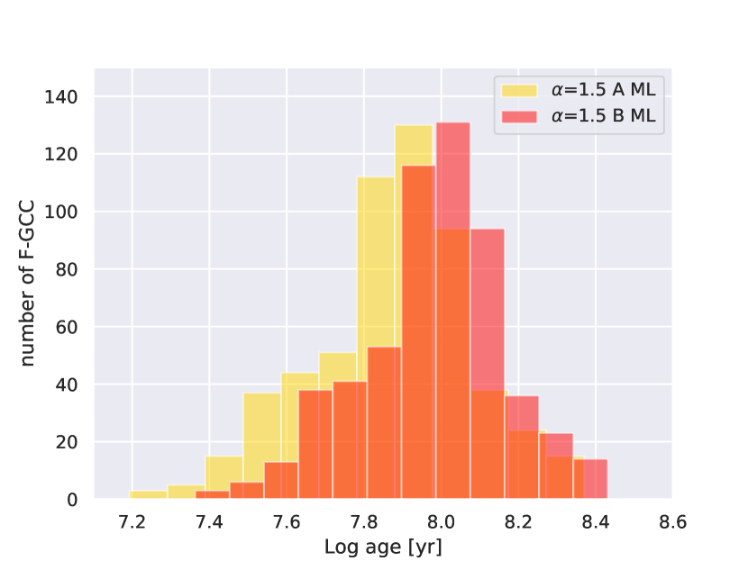
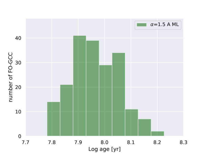
Figure 10: The predicted age distribution as obtained by applying the PAC relation to the selected sample of F (left panel) and FO-mode (right panel) GCC, for the labelled assumptions on the efficiency of superadiabatic convection and ML relation

4.1 The age map distribution of Gaia DR2 Cepheids

The possibility of retrieving accurate and reliable age estimates of a large sample of GCC by using the PA and/or the PAC relationships provides the opportunity to perform an age tomography of the Galaxy, and hence to properly trace the Star Formation history of the various portions of the Milky Way, in particular, in the regime of young and intermediate ages.

In order to show the inferred GCC age distribution as a function of the position in the Galactic disk, the selected Gaia DR2 Cepheid sample was represented in the Galactic coordinates with the predicted individual age varying according to the logarithmic color-bar scale and increasing from blue to red.

The maps shown in Figure 11 refer to F and FO-mode GCC with ages derived from the PAC relations. From left to right, the panels show the age map for: F-mode GCC by assuming the ML case A, F-mode GCC by assuming the ML case B and FO-mode GCC by assuming the ML case A. In all panels, the pulsation predictions were based on an adopted mixing length equal to $\alpha_{ml}~{}$=$1.5$. Inspection of these figures suggests that:

• the predicted ages decrease towards the Galactic center, with the oldest Cepheids located at longer Galactocentric distances.

• for the same assumption on the ML relation, FO-mode Cepheids are found to be systematically older than the F ones.

Although a detailed analysis of this topic is out of the aims of the present investigation, both the age and the spatial distributions of the CC in our sample as a function of their age can be compared with independent studies on the presence of age gradients among the various stellar populations in the Milky Way. For example, Skowron et al. (2019), applied the PA relation by Anderson et al. (2016) to the OGLE database of GCC, and found an age distribution (see their Figure 3) very similar to our results based on PA and PAC relations obtained from case B models. Recently, Bossini et al. (2019) computed the age distribution of 269 Galactic open clusters with astrometric and photometric data from Gaia DR2. However, in this case the possibility of realizing a meaningful comparison is hampered by the fact that the open cluster sample adopted by Bossini et al. (2019) spans an age range limited with respect to that of the GCC sample adopted in the present investigation.

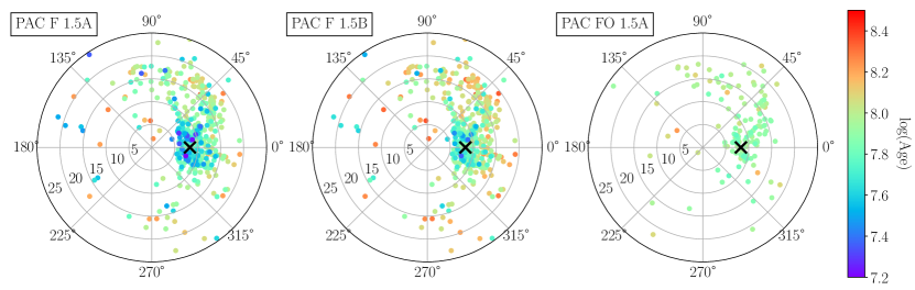
Figure 11: Distribution of the selected Gaia DR2 Cepheids on the Galactic plane plotted in polar coordinates. The Galactic center is in the middle. The Galactocentric polar coordinate is 0$\degr$ in the direction of the Sun, whose position is marked by a black cross. Each circle shows Galactocentric distances increasing by 5 kpc, from 0 up to 25 kpc. In each panel the colored circles show the predicted individual ages as obtained by using the PAC relations, according to the logarithmic color-bar axis. The labels on the top-left of each figure indicate the pulsation mode, while 1.5 A or B refer to the PAC obtained by assuming $\alpha_{ml}~{}$=$1.5$ and canonical and non canonical stellar models, respectively.

5 Conclusions and Future Developments

The most recent updated evolutionary predictions for the solar chemical composition based on the BASTI stellar evolution database (Hidalgo et al., 2018) were combined with the recent nonlinear convective Cepheid models developed by DS20. This was done to derive updated and accurate PA relations, as well as the first PAC relations in the Gaia DR2 photometric passbands, for various assumptions about the ML relations and the efficiency of superadiabatic convection in pulsation models.

The coefficients of these relations and hence, the corresponding age predictions, significantly depend on the assumed ML relations with the non canonical ML relation (case B in the present work) providing ages older than the canonical ML (case A) relation. For the case of PA relations, in particular, the predicted age difference percentages inferred from case A to case B, range from $\sim$ 36 % to $\sim$ 60 %. This trend is confirmed by the behaviour of the PAC relations.

The application of the new PA and Gaia-band PAC relations to a selected sample (Ripepi et al., 2019) of Gaia DR2 GCC, produces individual ages which systematically increase as the ML relation changes from canonical (case A) to non canonical (case B) models. When adopting case A ML models, the inferred age distribution of F-mode GCC in our sample peaks at around 90 Myr, while for case B the peak is shifted upwards by $\sim 35$ Myr. This occurrence holds when adopting both the PA and the PAC relations.

On the other hand, the age estimates obtained by means of both the PA and PAC relations are almost insensitive to variations in the mixing length parameter. This result is expected because a variation in the efficiency of superadiabatic convection can modify the pulsation amplitude and the boundary of the IS (see e.g. ; , and references therein), but does not affect at all the relation between period, color and luminosity; and hence, the relation between period, color and age.

The FO-mode GCC from the sample by Ripepi et al. (2019) are found to be significantly older than the average F pulsator age distribution. This is due to the smaller masses and shorter periods of the FO pulsators.

We have performed a preliminary comparison between the age map distribution obtained in the present work with other similar analyses in literature. In general, we found that older Cepheids are located at a longer Galactocentric distance than younger pulsators, an occurrence in fine agreement with previous results for the age distribution of Milky Way CC obtained by Skowron et al. (2019).

A more detailed analysis of the inferences that can be obtained from the star formation history of the various portions of our Galaxy at different locations from the study of the age distribution of CC, does need to be supplemented with an accurate investigation of the metallicity distribution of these pulsators. We plan to extend in a future research the present theoretical investigation to different metallicity regimes in order to properly account for the whole metallicity distribution of Galactic Cepheids.

References

- Anderson et al. (2016) Anderson R. I., Saio H., Ekström S., Georgy C., Meynet G., 2016, A&A, 591, A8
- Bergemann & Serenelli (2014) Bergemann M., Serenelli A., 2014, Solar Abundance Problem. pp 245–258, doi:10.1007/978-3-319-06956-2_21
- Böhm-Vitense (1958) Böhm-Vitense E., 1958, Z. Astrophys., 46, 108
- Bono & Stellingwerf (1994) Bono G., Stellingwerf R. F., 1994, ApJS, 93, 233
- Bono et al. (2000a) Bono G., Castellani V., Marconi M., 2000a, ApJ, 529, 293
- Bono et al. (2000b) Bono G., Caputo F., Cassisi S., Marconi M., Piersanti L., Tornambè A., 2000b, ApJ, 543, 955
- Bono et al. (2005) Bono G., Marconi M., Cassisi S., Caputo F., Gieren W., Pietrzynski G., 2005, ApJ, 621, 966
- Bossini et al. (2019) Bossini D., et al., 2019, A&A, 623, A108
- Caffau et al. (2011) Caffau E., Ludwig H.-G., Steffen M., Freytag B., Bonifacio P., 2011, Sol. Phys., 268, 255
- Caputo et al. (2005) Caputo F., Bono G., Fiorentino G., Marconi M., Musella I., 2005, ApJ, 629, 1021
- Catelan & Smith (2015) Catelan M., Smith H. A., 2015, Pulsating Stars
- Cox & Giuli (1968) Cox J. P., Giuli R. T., 1968, Principles of stellar structure
- De Somma et al. (2020) De Somma G., Marconi M., Molinaro R., Cignoni M., Musella I., Ripepi V., 2020, ApJS, 247, 30
- Efremov (1978) Efremov I. N., 1978, Soviet Ast., 22, 161
- Efremov (2003) Efremov Y. N., 2003, Astronomy Reports, 47, 1000
- Efremov & Elmegreen (1998) Efremov Y. N., Elmegreen B. G., 1998, MNRAS, 299, 588
- Fiorentino et al. (2007) Fiorentino G., Marconi M., Musella I., Caputo F., 2007, A&A, 476, 863
- Fiorentino et al. (2013) Fiorentino G., Musella I., Marconi M., 2013, MNRAS, 434, 2866
- Gaia Collaboration et al. (2018) Gaia Collaboration et al., 2018, A&A, 616, A1
- Grebel & Brandner (1998) Grebel E. K., Brandner W., 1998, in Magellanic Clouds and Other Dwarf Galaxies. pp 151–154
- Grevesse & Sauval (1998) Grevesse N., Sauval A. J., 1998, Space Sci. Rev., 85, 161
- Groenewegen (2018) Groenewegen M. A. T., 2018, A&A, 619, A8
- Hidalgo et al. (2018) Hidalgo S. L., et al., 2018, ApJ, 856, 125
- Inno et al. (2015) Inno L., et al., 2015, The Recent Star Formation History of the Magellanic Clouds Traced by Classical Cepheids. p. 265
- Lodders (2010) Lodders K., 2010, Astrophysics and Space Science Proceedings, 16, 379
- Magnier et al. (1997) Magnier E. A., Augusteijn T., Prins S., van Paradijs J., Lewin W. H. G., 1997, A&AS, 126, 401
- Marconi et al. (2005) Marconi M., Musella I., Fiorentino G., 2005, ApJ, 632, 590
- Marconi et al. (2006) Marconi M., Bono G., Caputo F., Cassisi S., Pietrukowicz P., Pietrzynski G., Gieren W., 2006, Mem. Soc. Astron. Italiana, 77, 67
- Marconi et al. (2013) Marconi M., et al., 2013, ApJ, 768, L6
- Pietrinferni et al. (2004) Pietrinferni A., Cassisi S., Salaris M., Castelli F., 2004, ApJ, 612, 168
- Reimers (1975) Reimers D., 1975, Memoires of the Societe Royale des Sciences de Liege, 8, 369
- Renzini et al. (1992) Renzini A., Greggio L., Ritossa C., Ferrario L., 1992, ApJ, 400, 280
- Riess et al. (2011) Riess A. G., et al., 2011, ApJ, 730, 119
- Riess et al. (2019) Riess A. G., Casertano S., Yuan W., Macri L. M., Scolnic D., 2019, ApJ, 876, 85
- Ripepi et al. (2017) Ripepi V., et al., 2017, MNRAS, 472, 808
- Ripepi et al. (2019) Ripepi V., Molinaro R., Musella I., Marconi M., Leccia S., Eyer L., 2019, A&A, 625, A14
- Salaris & Cassisi (2006) Salaris M., Cassisi S., 2006, Evolution of Stars and Stellar Populations
- Salaris & Cassisi (2008) Salaris M., Cassisi S., 2008, A&A, 487, 1075
- Senchyna et al. (2015) Senchyna P., et al., 2015, ApJ, 813, 31
- Skowron et al. (2019) Skowron D. M., et al., 2019, Science, 365, 478
- Tammann et al. (2003) Tammann G. A., Sandage A., Reindl B., 2003, A&A, 404, 423
- Tsvetkov (1980) Tsvetkov T. G., 1980, Soviet Astronomy Letters, 6, 400
- Udalski et al. (2018) Udalski A., et al., 2018, Acta Astron., 68, 315
- Wood (2006) Wood P. R., 2006, Mem. Soc. Astron. Italiana, 77, 76