Frictionless motion of lattice defects

Abstract

Energy dissipation by fast crystalline defects takes place mainly through the resonant interaction of their cores with periodic lattice. We show that the resultant effective friction can be reduced to zero by appropriately tuned acoustic sources located on the boundary of the body. To illustrate the general idea, we consider three prototypical models describing the main types of strongly discrete defects: dislocations, cracks and domain walls. The obtained control protocols, ensuring dissipation-free mobility of topological defects, can be also used in the design of meta-material systems aimed at transmitting mechanical information.

Mobile crystalline defects respond to lattice periodicity by dynamically adjusting their core structure which leads to radiation of lattice waves through parametric resonance Currie et al. (1977); Peyrard and Kruskal (1984); Kunz and Combs (1985); Boesch et al. (1989); Kevrekidis et al. (2002). Such ’hamiltonian damping’ is one of the main mechanisms of energy loss for fast moving dislocations Atkinson and Cabrera (1965); Kresse and Truskinovsky (2004), crack tips Slepyan (1981); Marder and Gross (1995) and elastic phase/twin boundaries Slepyan (2001); Truskinovsky and Vainchtein (2005). Similar effective dissipation hinders the mobility of topological defects in mesoscopic dispersive systems, from periodically modulated compositesDohnal et al. (2015) to discrete acoustic metamaterials Kochmann and Bertoldi (2017).

While at the macroscale friction is usually diminished by applying lubricants, at the microscale it may be preferable to use instead external sources of ultrasound (sonolubricity) Pfahl et al. (2018). Correlated mechanical vibrations are known to reduce macroscopic friction through acoustic ‘unjamming’ Capozza et al. (2009) as in the case of the remote triggering of earthquakes de Arcangelis et al. (2019). General detachment front tips serve as macroscopic defects whose mobility in highly inhomogeneous environments can be controlled by AC (alternating current) driving Rubinstein et al. (2004). Ultrasound-induced lubricity can also reduce friction at the microscale Dinelli et al. (1997). It is known, for instance, that the forming load drops significantly in the presence of appropriately tuned time-periodic driving which reduces dislocation friction Winsper et al. (1970).

The AC-based control of the directed transport in damped systems was studied extensively for the case when the sources are distributed in the bulk Bonilla and Malomed (1991); Cai et al. (1994); Baizakov et al. (2007). In this Letter we neglect the conventional bulk dissipation, associated for instance, with ’phonon wind’ Koizumi et al. (2002), and show how in purely Hamiltonian setting the effective friction can be tuned to zero by the special AC driving acting on the system boundary Tshiprut et al. (2005); Capozza et al. (2011).

Since classical continuum models lack the resolution to describe dynamic defect cores and therefore cannot capture adequately the interaction between the defect and the external micro-structure, we use atomistic models accounting for the coupling between the defect and the lattice vibrations while respecting the anharmonicity of interatomic forces. We build upon the theoretical methodology developed in Slepyan (2001); Mishuris et al. (2009); Nieves et al. (2017) and show that such driving can compensate radiative damping completely, making the discrete system fully transparent for mobile topological defects.

To highlight ideas we present a comparative study of the three prototypical snapping-bond type lattice models originating in crystal plasticity (Frenkel-Kontorova (FK) model Kresse and Truskinovsky (2004)), theory of structural phase transitions (bi-stable Fermi-Pasta-Ulam (FPU) model Efendiev and Truskinovsky (2010)) and fracture mechanics (Peyrard-Bishop (PB) model, Maddalena et al. (2009)).

In the individual setting of each of these models we study the effect of the boundary AC sources on kinetic/mobility laws for the corresponding lattice defects. The latter relate the macroscopic driving force (dynamic generalization of the Peach-Koehler force in the case of dislocations, the stress intensity factor in the case of cracks and the Eshelby force in the case of phase boundaries) and the velocity of the defect. We find that in the presence of AC sources such relations becomes multivalued. We focus particularly on designing the AC protocols which ensure that the steady propagation of a defect takes place under zero driving force.

The possibility of externally guided radiation-free propagation of mechanical information is presently of considerable interest for designing discrete meta-materials with buckling linkages. Geometric phase transitions generating information-carrying defects in such systems play a central role in a multitude of new applications from recoverable energy harvesting to controlled structural collapse Shan et al. (2015); Zhang et al. (2019); Harne and Wang (2017).

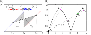
Figure 1: (a) Piece-wise linear stress-strain relation $\sigma=\sigma(\varepsilon)$; the macroscopic driving force $G^{M}(V)=S_{2}-S_{1}$. (b) Dispersion relation $\omega(k)$ for $\text{Im}(k)=0$ (acoustic branch); $k_{j}$ correspond to the radiated waves in cases $K=1$ and $K=3$, see the text. Green circles correspond to AC sources behind the defect, magenta squares - ahead of the defect.

The FPU model with bi-stable interactions is used to represent the simplest crystal defect, a domain wall Truskinovsky and Vainchtein (2005); Slepyan et al. (2005). In terms of dimensionless particle displacements $u_{j}(t)$ the dynamics is described by the system

$$\ddot{u}_{j}(t)=\sigma\left(u_{j+1}-u_{j}\right)-\sigma\left(u_{j}-u_{j-1}\right).$$ (1)

It will be convenient to use strain variables $\varepsilon_{j}(t)=u_{j+1}(t)-u_{j}(t)$ and introduce the strain energy density $w(\varepsilon)$ so that $\sigma(\varepsilon_{j})=w^{\prime}(\varepsilon_{j})$. For analytical transparency we adopt the simplest bi-quadratic model with $w=(1/2)\varepsilon^{2}-\sigma_{0}(\varepsilon-\varepsilon_{c})H(\varepsilon-\varepsilon_{c})$, where $H(x)$ is the Heaviside function, $\varepsilon_{c}$ is the characteristic strain and $\sigma_{0}$ is the stress drop, see Fig. 1(a).

We search for traveling wave (TW) solutions of (1) in the form $u_{j}(t)=u(\eta)$ and $\varepsilon_{j}=\varepsilon(\eta)$, where $\eta=j-Vt$ and $V<1$ is the normalized velocity of the defect. If we associate the defect with $\eta=0$ the equation for the strain field reduces to $V^{2}d^{2}\varepsilon/d\eta^{2}=\sigma(\eta+1)+\sigma(\eta-1)-2\sigma(\eta),$ where $\sigma(\eta)=\varepsilon(\eta)-\sigma_{0}H(-\eta).$ When this linear equation is solved, the velocity $V$ is found from the nonlinear switching condition $\varepsilon(0)=\varepsilon_{c}$.

Using the Fourier transform $\hat{f}(k)=\int_{-\infty}^{\infty}f(\eta)e^{ik\eta}\,d\eta$, we can rewrite the main linear problem in the form $L(k)\hat{\varepsilon}(k)=\sigma_{0}\omega^{2}(k)/(0+ik)$, where $L(k)\equiv\omega^{2}(k)-(kV)^{2}$ and $\omega^{2}(k)=4\sin^{2}{(k/2)}$ is the dispersion relation represented in this case by a single acoustic branch, see Fig. 1(b). The strain field $\varepsilon(\eta)$ can be decomposed into a sum of the term $\varepsilon_{in}(\eta)$, which is due to inhomogeneity (mimicking nonlinearity) and the term $\varepsilon_{dr}(\eta)$, due to the combined action of DC (direct current) and AC driving. The former can be written explicitly

$$\varepsilon_{in}(\eta)=\frac{\sigma_{0}}{2\pi}\int_{-\infty}^{\infty}\frac{\omega^{2}(k)e^{-ik\eta}}{(0+ik)L(k)}\,dk.$$ (2)

The latter must satisfy $L(k)\hat{\varepsilon}_{dr}(k)=0$ which in the physical space gives

$$\varepsilon_{dr}(\eta)=\sum_{j=1}^{K}A_{j}\sin{(k_{j}\eta+\varphi_{j})}+C.$$ (3)

The constants $A_{j}$ and $\varphi_{j}$ describe the amplitude and the phase of the incoming waves generated at the distant boundaries. They represent the AC driving which is characterized by the wave numbers $k_{j}$ that are taken among the positive real roots of the kernel $L(k)$: if $\omega^{\prime}(k_{j})$ is smaller (greater) than $V$ the sources are in front of (behind) the moving defect. The constant $C$ in (3), representing the root $k_{0}=0$, controls the uniform strain ahead of the moving defect and represents the DC driving.

Use the switching condition we can obtain the explicit relations for the limiting strains in the form $\langle\varepsilon\rangle(\pm\infty)\equiv\varepsilon_{\pm}=\varepsilon_{c}\mp\frac{1}{2}\frac{\sigma_{0}}{1-V^{2}}+\sigma_{0}Q-\sum_{j=1}^{K}A_{j}\sin{\varphi_{j}},$ where $\langle f\rangle=\lim_{T\to\infty}(1/T)\int_{0}^{T}f(s)ds$ and the expression for the universal function $Q(V)$ can be found in SOM . It can be checked that the obtained solution respects the macroscopic momentum balance represented by one of the Rankine-Hugoniot (RH) conditions Dafermos et al. (2005): $V^{2}=(\sigma(\varepsilon_{+})-\sigma(\varepsilon_{-}))/(\varepsilon_{+}-\varepsilon_{-})$. The limiting values of the mass velocity $v_{j}=\dot{u}_{j}$ naturally satisfy another (kinematic) RH condition $\langle v\rangle(\pm\infty)\equiv v_{\pm}=-V\varepsilon_{\pm}$.

We now write the macroscopic energy dissipation on the moving defects as $\mathcal{R}=VG\geq 0$ where $G$ is the driving force. In the absence of the AC driving ($A_{j}=0$) we obtain $G=G^{M}$, where

$$G^{M}=\llbracket{w}\rrbracket-\{\sigma\}\llbracket\varepsilon\rrbracket,$$ (4)

and we used the standard notations $\llbracket f\rrbracket=f_{+}-f_{-}$ and $\{f\}=(f_{+}+f_{-})/2$ Truskinovsky (1987). In our case $G^{M}=(\sigma_{0}/2)(\varepsilon_{+}+\varepsilon_{-}-2\varepsilon_{c})$. With the AC driving present, we need to write $\mathcal{R}=V(G^{M}+G^{m})\geq 0$ where the total power exerted by microscopic sources is

$$VG^{m}=\sum_{j=1}^{K}(1/2)A_{j}^{2}\left|\omega^{\prime}(k_{j})-V\right|\geq 0.$$ (5)

The relation for $\mathcal{R}$ can be checked by the independent computation of the energy carried by the microscopic radiation away from the moving defect to infinity SOM .

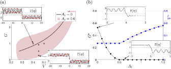
Figure 2: (a) Kinetic domain for the case $K=1$, open squares show the selected TW solutions reached numerically SOM ; (b) Amplitude dependence of $G^{*}$ and $V^{*}$; insets show normalized strains $\overline{\varepsilon}(\eta)=\varepsilon(\eta)/\varepsilon_{c}$. Parameters: $\sigma_{0}=2,\,\varepsilon_{c}=1$.

The dependence of $G$ on $V$ for a high velocity subset of admissible solutions is shown in Fig. 2(a). The radiative damping is represented here by a single wave number $k_{1}$. The AC driving is tuned to the same wave number and its source is placed ahead of the moving defect (the $K=1$ regime). If the AC driving is absent and all $A_{j}=0$, there is a single value of $V$ for each value of $G$ within the admissible range $\pm(\varepsilon_{c}-\varepsilon(\eta))>0$ at $\pm\eta>0$. Even if only one coefficient $A_{1}\neq 0$, each admissible value of velocity $V$ can be reached within a finite range of DC driving amplitudes with the associated phase shift $\varphi_{1}$ varying continuously. In this case the kinetic relation transforms into a 2D kinetic domain, see Fig. 2(a), where by fixing the DC drive we can either speed up or slow down the defect as we change the frequency of the AC source.

The possibility of the AC induced friction reduction is seen from the fact that for each $V$ there is a range of the admissible driving forces $G$ with the minimal value $G^{*}(V)$. Moreover, for some $V^{*}$ such friction can be eliminated completely if the amplitude $A_{1}$ reaches beyond a threshold. Note that the emergence of friction-free regimes resembles a second order phase transition with the dissipation $G^{*}$ as the order parameter, see Fig. 2(b). The non-dissipative regimes with $K=1$ are naturally anti-phase with respect to the radiated waves so that $\varphi_{1}^{*}=\pi/2$, see a typical strain distribution in the insets in Fig. 2(b) and Fig. 3. The relation between the AC amplitude and the defect velocity for such regimes can be written explicitly $A_{1}^{*}=\sigma_{0}V/(V-\omega^{\prime}(k_{f})).$

In the general case $K\neq 1$ the number of dissipative waves is odd and the dissipation-free regimes also must have an odd number of AC sources to cancel each of these waves. Consider, for instance, the case $K=3$, illustrated in Fig. 1(b), where two dissipative lattice waves ($k_{1}$ and $k_{3}$) release energy at $-\infty$ and one wave ($k_{2}$) - at $+\infty$. To block these dissipative waves one must have the sources of AC driving both in front and behind the defect. The corresponding amplitudes, ensuring that $G^{*}(V)=0$, are $A^{*}_{j}=(-1)^{j}\sigma_{0}V/(\omega^{\prime}(k_{j})-V)$ with $j=1,2,3$, see Fig. 3.

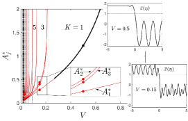
Figure 3: Amplitudes of the AC sources $A_{j}^{*}(V),\,j=1,2,..,K$ for $K=1,3,5...$; insets show strains $\overline{\varepsilon}(\eta)=\varepsilon(\eta)/\varepsilon_{c}$ at $V=0.15$ and $V=0.5$ with corresponding $A_{j}^{*}$ marked by solid circles. Black lines correspond to admissible solutions, red - to non admissible. Parameters: $\sigma_{0}=2,\,\varepsilon_{c}=1$.

The numerical check shows that the admissible frictionless regimes exist only for $K=1$. To show numerical stability of these regimes we simulated the transient problem with initial data close to the analytical TW solutions, see SOM for details. The simulation involving $1000$ equations and showing stable dissipation-free propagation of the defect is presented in the form of the supplementary Movie 2.

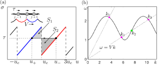
Figure 4: (a) Dislocation propagation driven by the constant force $\tau$; macroscopic driving force $G^{M}(V)=S_{2}-S_{1}$; (b) Dispersion relation for $\text{Im}(k)=0$ (optical branch). The wave numbers $k_{j}$ define radiated waves in the cases $K=1$ and $K=3$.

The simplest FK model Atkinson and Cabrera (1965); Kresse and Truskinovsky (2003) can be used to analyze the frictionless propagation regimes for moving dislocations, see Fig. 4(a). To describe a single dislocation we only need two wells of the on-site periodic potential. The displacement $u_{j}(t)$, describing horizontal slip, must solve the equations

$$\ddot{u}_{j}=u_{j-1}+u_{j+1}-2u_{j}-\sigma(u_{j})+\tau$$ (6)

where $\tau$ is a uniform load. The function $\sigma(u)$ is illustrated in Fig. 4(a) and is defined via the on-site potential $w(u)=(1/2)u^{2}$ when $-u_{c}<u<u_{c}$ and $w(u)=(1/2)u^{2}-\sigma_{0}(u-u_{c})$ when $u_{c}<u<3u_{c}$ representing the two relevant periods. We again use the TW ansatz $u_{j}(t)=u(\eta),\,\eta=j-Vt$ and apply the corresponding condition of admissibility. Unlike the previous case, the DC drive $\tau$ is now applied in the bulk.

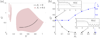
Figure 5: (a) Kinetic domains for dislocations showing admissible solutions with $K=1$. There is only one damping wave in the big pink domain and more than one in the smaller ones. (b) AC amplitude dependence of $G^{*}(V^{*})$ and $V^{*}$; insets show displacements $\overline{u}(\eta)=u(\eta)/u_{c}$. Parameters: $\sigma_{0}=2,\,u_{c}=1$.

We need to solve the linear equation $V^{2}u^{\prime\prime}(\eta)=u(\eta+1)+u(\eta-1)-3u(\eta)+\sigma_{0}H(-\eta)+\tau$ and then find the defect velocity $V$ using the nonlinear switching condition $u(0)=u_{c}$. The solution can be again represented in the form $u(\eta)=u_{in}(\eta)+u_{dr}(\eta)$. The first term, which is due to inhomogeneity (mimicking nonlinearity) now includes the DC driving $\tau$:

$$u_{in}(\eta)=\tau+\frac{\sigma_{0}}{2\pi}\int_{-\infty}^{\infty}\frac{e^{-ik\eta}}{(0+ik)L(k)}\,dk,$$ (7)

where the operator $L(k)$ remains the same as in the FPU problem but the dispersion relation $\omega^{2}(k)=4\sin^{2}(k/2)+1$ is now represented by a single optical branch. The second term responsible for the AC driving must again satisfy $L(k)\hat{u}_{dr}(k)=0$ and can be again represented as a combination of linear waves whose phase velocity is equal to $V$

$$u_{dr}(\eta)=\sum_{j=1}^{K}A_{j}\sin(k_{j}\eta+\varphi_{j}).$$ (8)

Here $k_{j}$ are again the positive real roots of $L(k)=0$.

Using the switching condition we obtain for the time averaged displacements at $\pm\infty$ the values $u_{\pm}=u_{c}\mp(\sigma_{0}/2)+\sigma_{0}R-\sum_{j}A_{j}\sin\varphi_{j}$ with the explicit expression for the universal function $R(V)$ is given again in SOM . The analogs of the RH conditions are now $u_{+}=\tau$ and $u_{-}=\tau+\sigma_{0}$.

If we denote the stress in the horizontal bonds by $\bar{\sigma}(\varepsilon)=\varepsilon$ we can write the rate of dissipation at the macro-scale as $VG^{M}=\llbracket v^{2}/2+\varepsilon^{2}/2+w-\tau u\rrbracket V+\llbracket\bar{\sigma}v\rrbracket$. Applying the kinematic RH condition $\llbracket v\rrbracket+V\llbracket\varepsilon\rrbracket=0$ we obtain

$$G^{M}=\llbracket w\rrbracket-\tau\llbracket u\rrbracket.$$ (9)

Since $\varepsilon_{\pm}=\bar{\sigma}(\varepsilon_{\pm})=0$ we can finally write the macroscopic driving force in the form $G^{M}=\sigma_{0}^{2}/2-\sigma_{0}(u_{c}-u_{+}).$ The contribution to the energy flux due to AC sources is now

$$VG^{m}=\sum_{j=1}^{K}(1/2)A_{j}^{2}\omega^{2}(k_{j})\left|\omega^{\prime}(k_{j})-V\right|\geq 0.$$ (10)

The multi-valued relation $\mathcal{R}(V)=VG(V)=G^{M}(V)+G^{m}(V)$ for admissible solutions is illustrated in Fig. 5(a) for the case $K=1$. It is again possible to completely cancel the lattice friction and obtain regimes with $G^{*}(V^{*})=0$. In such regimes, illustrated for $K=1$ in Fig. 5(b), the radiated waves are again annihilated by the waves generated by the AC source with the amplitudes $A_{j}^{*}=(-1)^{j}\sigma_{0}V/(\omega(k_{j})^{2}(\omega^{\prime}(k_{j})-V))$ and phase shifts $\varphi^{*}_{j}=\pi/2$.

Our last example deals with reversible fracture in the simplest PB-type setting Peyrard and Bishop (1989); Marder and Gross (1995); Maddalena et al. (2009). The lattice defect is now a crack tip moving under the action of a transversal force from left to right by consequently breaking the bonds represented by elastic fuses, see Fig. 6(a).

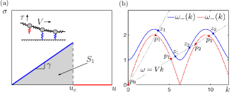
Figure 6: (a) Constitutive relation for a mechanical fuse and schematic representation of a crack propagating with velocity $V$ under remote load $\tau$; the strain energy jump $\llbracket w\rrbracket=-S_{1}$. (b) Dispersion relations $\omega_{+}(k)$ (optical branch) and $\omega_{-}(k)$ (acoustic branch) for $\text{Im}(k)=0$ characterizing intact and broken lattices, respectively.

The equations governing the evolution of the vertical displacements $u_{j}(t)$ are

$$\ddot{u}_{j}=u_{j-1}+u_{j+1}-2u_{j}-\gamma u_{j}H(u_{j}-u_{c})$$ (11)

see Fig. 6(a) for notations, and we again look for solutions in the TW form $u_{j}(t)=u(\eta),\,\eta=j-Vt$. We need to solve a linear equation $V^{2}u^{\prime\prime}(\eta)=u(\eta+1)+u(\eta-1)-2u(\eta)-\gamma u(\eta)H(\eta)$ and use the nonlinear switching condition $u(0)=u_{c}$ to find the defect velocity $V$. The dispersion relations are now represented by one optical branch $\omega_{+}^{2}(k)=4\sin^{2}{(k/2)}+\gamma$ ahead and one acoustic branch $\omega_{-}^{2}(k)=4\sin^{2}{(k/2)}$ behind the defect.

One way to solve this more complex problem is to use the Wiener-Hopf technique, see SOM for details. We can again obtain the decomposition $u(\eta)=u_{in}(\eta)+u_{dr}(\eta)$, but now to define different terms we need to introduce two auxiliary functions $L^{\pm}(k)=L^{\mp 1/2}(k)\exp{(\frac{1}{2\pi i}\int_{-\infty}^{\infty}\frac{\text{Log }L(\xi)}{k-\xi}d\xi)},$ where $L(k)\equiv(\omega_{+}^{2}(k)-(kV)^{2})/(\omega_{-}^{2}(k)-(kV)^{2})$. Then

$$u_{in}(\eta)=\frac{C}{2\pi}\int_{-\infty}^{\infty}\frac{L^{\pm}(k)e^{-ik\eta}}{0\mp ik}\,dk,\quad\pm\eta>0$$ (12)

is the contribution due to remotely applied DC force $\tau$ which is modeled by the condition that at $\eta=-\infty$ the time average displacements follows the asymptotics $u(\eta)\sim-\tau\eta$, while at $\eta=+\infty$ the average displacements tend to zero. From these conditions we find that $C=\tau S\sqrt{(1-V^{2})/\gamma}$ where an explicit expression for the function $S(V)$ is given in SOM . The contribution due to the AC driving is

$$u_{dr}(\eta)=\frac{1}{2\pi}\int_{-\infty}^{\infty}L^{\pm}(k)\Psi_{dr}^{\pm}(k)e^{-ik\eta}\,dk,\quad\pm\eta>0$$ (13)

where

$$\Psi_{dr}^{\pm}(k)=\sum_{j=1}^{K}\frac{A_{j}}{2}\left[\frac{e^{-i(\varphi_{j}-\pi/2)}}{0\mp i(k-k_{j})}+\frac{e^{i(\varphi_{j}-\pi/2)}}{0\mp i(k+k_{j})}\right].$$ (14)

Here the wave numbers $k_{j}=z_{2j-1}$ describe the sources bringing the energy from $+\infty$ while the wave numbers $k_{j}=p_{2j}$ correspond to sources bringing the energy from $-\infty$; for the cases $K=1,3$ the wave numbers $z$ and $p$ are illustrated in Fig. 6(b).

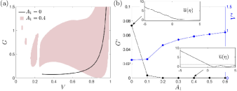
Figure 7: (a) Kinetic domains for admissible solutions with $K=1$ and the AC wave coming from ahead. There is only one damping wave in the big pink domain and more than one in the smaller ones. (b) Amplitude dependence of $G^{*}(V^{*})$ and $V^{*}$. Material properties are $\gamma=1,\,u_{c}=1$.

To compute the driving force $G^{M}$ we observe that the macroscopic energy dissipation on the crack tip is $VG^{M}=\llbracket v^{2}/2+\varepsilon^{2}/2+w\rrbracket V+\llbracket\bar{\sigma}v\rrbracket$, where $w(u)=(1/2)\gamma u^{2}$ for $u<u_{c}$ and $w(u)=(1/2)\gamma u_{c}^{2}$ for $u>u_{c}$. If we now take into consideration the RH compatibility condition $\llbracket v\rrbracket+V\llbracket\varepsilon\rrbracket=0$, we obtain $VG^{M}=\llbracket w\rrbracket V+\bar{f}\{v\}$. Here $\bar{f}=\llbracket\bar{\sigma}\rrbracket-V^{2}\llbracket\varepsilon\rrbracket$ is the moving concentrated force which represents the microscopic processes in the tip and furnishes the linear momentum RH condition, e.g. Burridge and Keller (1978). We can now write

$$G^{M}=\llbracket w\rrbracket-\bar{f}\llbracket\varepsilon\rrbracket$$ (15)

and substituting the values $\varepsilon_{-}=-\tau$, $\varepsilon_{+}=0$, $\bar{\sigma}(\varepsilon_{\pm})=\varepsilon_{\pm},$ we finally obtain $G^{M}=\tau^{2}(1-V^{2})/2-(\gamma u_{c}^{2})/2.$

Consider the simplest case when there is only one radiated wave with $k_{1}=p_{1}$. The microscopic power exerted by a single AC source ahead of the crack ($K=1$) is then

$$VG^{m}=\frac{1}{2}A_{1}^{2}\omega^{2}_{+}(z_{1})|L^{+}(z_{1})|^{2}\left|\omega_{+}^{\prime}(z_{1})-V\right|\geq 0.$$ (16)

The total dissipation $\mathcal{R}(V)=VG(V)=V(G^{M}(V)+G^{m}(V))\geq 0$ is again a multivalued function of $V$ as we show in Fig. 7(a); the associated functions $G^{*}(V^{*})$ and $V^{*}$ at different values of $A_{1}$ are shown in Fig. 7(b). At a given $V$ we obtain $A^{*}_{1}=u_{c}(z_{1}^{2}-p_{1}^{2})/z_{1}^{2}$ and $\varphi^{*}_{1}=\pi/2$ with the corresponding dissipation-free solution illustrated in the inset in Fig. 7(b). More general solutions, similar to the ones in Fig. 3, can be obtained as well.

To conclude, we showed that it is possible to fine tune defect kinetics by carefully engineered AC driving. Moreover, using special AC sources on the boundary, one can compensate radiative damping completely, making the crystal free of internal friction for strongly discrete defects. We demonstrated this effect for domain boundaries, dislocations and cracks, however, the obtained results also have important implications for the design of artificial metamaterials supporting mobile topological defects and capable of transporting compact units of mechanical information.

References

- Currie et al. (1977) J. Currie, S. Trullinger, A. Bishop, and J. Krumhansl, Physical Review B 15, 5567 (1977).
- Peyrard and Kruskal (1984) M. Peyrard and M. D. Kruskal, Physica D: Nonlinear Phenomena 14, 88 (1984).
- Kunz and Combs (1985) C. Kunz and J. A. Combs, Physical Review B 31, 527 (1985).
- Boesch et al. (1989) R. Boesch, C. Willis, and M. El-Batanouny, Physical Review B 40, 2284 (1989).
- Kevrekidis et al. (2002) P. Kevrekidis, I. Kevrekidis, A. Bishop, and E. Titi, Physical Review E 65, 046613 (2002).
- Atkinson and Cabrera (1965) W. Atkinson and N. Cabrera, Physical Review 138, A763 (1965).
- Kresse and Truskinovsky (2004) O. Kresse and L. Truskinovsky, Journal of the Mechanics and Physics of Solids 52, 2521 (2004).
- Slepyan (1981) L. I. Slepyan, in Doklady Akademii Nauk (Russian Academy of Sciences, 1981), vol. 258, pp. 561–564.
- Marder and Gross (1995) M. Marder and S. Gross, Journal of the Mechanics and Physics of Solids 43, 1 (1995).
- Slepyan (2001) L. I. Slepyan, Journal of the Mechanics and Physics of Solids 49, 469 (2001).
- Truskinovsky and Vainchtein (2005) L. Truskinovsky and A. Vainchtein, SIAM Journal on Applied Mathematics 66, 533 (2005).
- Dohnal et al. (2015) T. Dohnal, A. Lamacz, and B. Schweizer, Asymptotic Analysis 93, 21 (2015).
- Kochmann and Bertoldi (2017) D. M. Kochmann and K. Bertoldi, Applied Mechanics Reviews 69 (2017).
- Pfahl et al. (2018) V. Pfahl, C. Ma, W. Arnold, and K. Samwer, Journal of Applied Physics 123, 035301 (2018).
- Capozza et al. (2009) R. Capozza, A. Vanossi, A. Vezzani, and S. Zapperi, Physical Review Letters 103, 085502 (2009).
- de Arcangelis et al. (2019) L. de Arcangelis, E. Lippiello, M. Pica Ciamarra, and A. Sarracino, Philosophical Transactions of the Royal Society A 377, 20170389 (2019).
- Rubinstein et al. (2004) S. M. Rubinstein, G. Cohen, and J. Fineberg, Nature 430, 1005 (2004).
- Dinelli et al. (1997) F. Dinelli, S. Biswas, G. Briggs, and O. Kolosov, Applied Physics Letters 71, 1177 (1997).
- Winsper et al. (1970) C. Winsper, G. Dawson, and D. Sansome, Metals Materials 4, 158 (1970).
- Bonilla and Malomed (1991) L. L. Bonilla and B. A. Malomed, Physical Review B 43, 11539 (1991).
- Cai et al. (1994) D. Cai, A. Bishop, N. Grønbech-Jensen, and B. A. Malomed, Physical Review E 50, R694 (1994).
- Baizakov et al. (2007) B. B. Baizakov, G. Filatrella, and B. A. Malomed, Physical Review E 75, 036604 (2007).
- Koizumi et al. (2002) H. Koizumi, H. Kirchner, and T. Suzuki, Physical Review B 65, 214104 (2002).
- Tshiprut et al. (2005) Z. Tshiprut, A. Filippov, and M. Urbakh, Physical Review Letters 95, 016101 (2005).
- Capozza et al. (2011) R. Capozza, S. M. Rubinstein, I. Barel, M. Urbakh, and J. Fineberg, Physical Review Letters 107, 024301 (2011).
- Mishuris et al. (2009) G. S. Mishuris, A. B. Movchan, and L. I. Slepyan, Journal of the Mechanics and Physics of Solids 57, 1958 (2009).
- Nieves et al. (2017) M. Nieves, G. Mishuris, and L. Slepyan, International Journal of Solids and Structures 112, 185 (2017).
- Efendiev and Truskinovsky (2010) Y. R. Efendiev and L. Truskinovsky, Continuum Mechanics and Thermodynamics 22, 679 (2010).
- Maddalena et al. (2009) F. Maddalena, D. Percivale, G. Puglisi, and L. Truskinovsky, Continuum Mechanics and Thermodynamics 21, 251 (2009).
- Shan et al. (2015) S. Shan, S. H. Kang, J. R. Raney, P. Wang, L. Fang, F. Candido, J. A. Lewis, and K. Bertoldi, Advanced Materials 27, 4296 (2015).
- Zhang et al. (2019) Y. Zhang, B. Li, Q. Zheng, G. M. Genin, and C. Chen, Nature Communications 10, 1 (2019).
- Harne and Wang (2017) R. L. Harne and K.-W. Wang, Harnessing bistable structural dynamics: for vibration control, energy harvesting and sensing (John Wiley & Sons, 2017).
- Slepyan et al. (2005) L. Slepyan, A. Cherkaev, and E. Cherkaev, Journal of the Mechanics and Physics of Solids 53, 407 (2005).
- (34) See Supplemental Material at [URL will be inserted by publisher] for [give brief description of material].
- Dafermos et al. (2005) C. M. Dafermos, C. M. Dafermos, C. M. Dafermos, G. Mathématicien, C. M. Dafermos, and G. Mathematician, Hyperbolic conservation laws in continuum physics, vol. 3 (Springer, 2005).
- Truskinovsky (1987) L. Truskinovsky, Journal of Applied Mathematics and Mechanics 51, 777 (1987).
- Kresse and Truskinovsky (2003) O. Kresse and L. Truskinovsky, Journal of the Mechanics and Physics of Solids 51, 1305 (2003).
- Peyrard and Bishop (1989) M. Peyrard and A. R. Bishop, Physical review letters 62, 2755 (1989).
- Burridge and Keller (1978) R. Burridge and J. Keller, SIAM Review 20, 31 (1978).