Conditional independence testing via weighted partial copulas and nearest neighbors

Abstract

This paper introduces the weighted partial copula function for testing conditional independence. The proposed test procedure results from these two ingredients: (i) the test statistic is an explicit Cramer-von Mises transformation of the weighted partial copula, (ii) the regions of rejection are computed using a bootstrap procedure which mimics conditional independence by generating samples from the product measure of the estimated conditional marginals. Under mild conditions on the estimated conditional marginals, rates of convergence for the weighted partial copula process and the test statistic are established. These high-level conditions are shown to be valid for the popular nearest neighbors estimate. Finally, an experimental section demonstrates that the proposed test has competitive power compared to recent state-of-the-art methods such as kernel-based test.

1 Introduction

Let $(Y_{1},Y_{2},X)$ be a triple of real random variables. We say that $Y_{1}$ and $Y_{2}$ are conditionally independent given $X$ if $\forall(y_{1},y_{2},x)\in\mathbb{R}^{3}$:

$$\Pr(Y_{1}\leq y_{1},\,Y_{2}\leq y_{2}\mid X=x)=\Pr(Y_{1}\leq y_{1}\mid X=x)\Pr(Y_{2}\leq y_{2}\mid X=x).$$ (1)

This is denoted by $Y_{1}\perp\perp Y_{2}~{}|~{}X$ and roughly speaking, it means that for a given value of $X$, the knowledge of $Y_{1}$ does not provide any further information on $Y_{2}$ (and vice versa). Determining conditional independence has become in the recent years a fundamental question in statistics and machine learning. For instance, it plays a key role in defining graphical models (Koller and Friedman, 2009; Bach and Jordan, 2003); see also Markowetz and Spang (2007) for a study specific to cellular networks. Moreover the concept of conditional independence lies at the core of sufficient dimension reduction methods (Li, 2018) and is useful to conduct variable selection in regression (Lee et al., 2016). Finally, conditional independence is relevant in many application fields such as economy (Huber and Melly, 2015) or psychometry (Bell et al., 1988). This paper proposes new statistical tests to assess conditional independence.

The approach taken is related to the well-studied problem of (unconditional) independence testing, in which the most intuitive way to proceed is perhaps to compute a distance between the estimated joint distribution and the product of the estimated marginals (Hoeffding, 1948). Inspired by Kendall (1948), rank-based statistics have been extensively used in independence testing (Ruymgaart, 1974; Ruschendorf, 1976; Ruymgaart and van Zuijlen, 1978). Because rank-based statistics do not depend on the marginals, they have appeared as a key tool for modelling the joint distribution of random variables without being affected by their margins. This has led to the introduction of the copula function (Deheuvels, 1981), defined as the cumulative distribution function associated to the ranks. We refer to Fermanian et al. (2004); Segers (2012) for recent studies on the estimation of the copula function. The copula function, which in principle measures the dependency between random variables has been used with success in independence testing (Genest and Rémillard, 2004; Genest et al., 2006). Because the asymptotic distribution of the copula function is difficult to estimate, the related bootstrap estimate properties are of prime interest for inference (Fermanian et al., 2004; Rémillard and Scaillet, 2009; Bücher and Dette, 2010).

The conditional copula of $Y_{1}$ and $Y_{2}$ given $X$ is defined in the same way as the copula of $Y_{1}$ and $Y_{2}$ but uses the conditional distribution of $Y_{1}$ and $Y_{2}$ given $X$ in place of the joint distribution of $Y_{1}$ and $Y_{2}$. Compared to the copula, the conditional copula captures the conditional dependency between random variables and is thus useful to build conditional dependency measures (Gijbels et al., 2011; Fukumizu et al., 2007; Derumigny and Fermanian, 2020). Therefore, as in the case of independence testing, the conditional copula appears to be a relevant tool for building statistical test of conditional independence. This has been pointed out as a an “interesting open issue” in (Veraverbeke et al., 2011, Section 4).

In this work, a new statistical test procedure, called the weighted partial copula test is investigated to assess conditional independence. The proposed approach follows from the use of an integrated criterion, the weighted partial copula, a function that equals $0$ if and only if conditional independence holds. Given estimators of the conditional marginals of $Y_{1}$ and $Y_{2}$ given $X$, the empirical weighted partial copula is introduced to estimate the weighted partial copula and the test statistic results from an easy-to-compute Cramer-von Mises transformation. The use of the weighted partial copula is motivated by the conditional moment restrictions literature (see Lavergne and Patilea (2013) and the reference therein) in which integrated criteria, similar to the weighted partial copula, have been frequently used. Those criteria are interesting because even when they involve local estimates converging at a slower rate than $1/\sqrt{n}$, their convergence rates are in many cases in $1/\sqrt{n}$.

Inspired by the independence testing literature (Beran et al., 2007; Kojadinovic and Holmes, 2009), the computation of the quantiles is made using a bootstrap procedure which generates bootstrap samples from the product of the marginal estimators to mimic the null hypothesis. Thanks to this bootstrap procedure, one is allowed to perform the weighted partial copula test using any marginal estimates as soon as one can generate from them.

The theoretical results of the paper are as follows. Under the uniform convergence of the estimated marginals, convergence rates are established for the empirical weighted partial copula and for the resulting test statistic. These results are interesting because they allow, in principle, to use any reasonable margins estimates when using the weighted partial copula test. A particular method that we promote is the flexible nearest neighbors approach. For this type of margins estimates, the uniform convergence condition is shown to be valid in a general framework. More specifically, we establish that the uniform error associated to the $k$-nearest neighbors estimate of the conditional margins is bounded by $1/\sqrt{k}+(k/n)^{1/d}$. This new result extends, in a non trivial way, previous works on nearest neighbors regression estimates (Biau et al., 2010; Jiang, 2019).

Related literature. Nonparametric testing for conditional independence has received an increasing interest the past few years (Li and Fan, 2020). Some of the existing approaches are based on comparing the (estimated) conditional distributions involved in the definition of conditional independence. The distributions can be compared using their conditional characteristic functions as in Su and White (2007), their conditional densities as proposed in Su and White (2008), or their conditional copulas as studied in Bouezmarni et al. (2012). Unfortunately, the estimation of these conditional quantities are subjected to the well-known curse of dimensionality, i.e., the convergence rates are badly affected by the dimension of the conditioning variable. As a consequence, the power of the previous tests rapidly deteriorates if the conditioning variable has a large dimension. Note also Bergsma (2010) that uses partial copulas to derive the test statistic. Unfortunately, partial copulas fail to capture the whole conditional distribution and lead to detect a null hypothesis much larger than conditional independence.

Other approaches rely on the characterization of conditional independence using cross-covariance operators defined on reproducing kernel Hilbert spaces (Fukumizu et al., 2004). Extending the Hilbert-Schmidt independence criterion proposed in Gretton et al. (2008), Zhang et al. (2011) defines a kernel-based conditional independence test (KCI-test) by estimating the cross-covariance operator. A surge of recent research (Doran et al., 2014; Runge, 2017; Sen et al., 2017) has focused on testing conditional independence using permutation-based tests. The work of Candes et al. (2018) had led to many conditional independence tests depending on the availability of an approximation to the distribution of $Y_{1}|X$, such as the conditional permutation test proposed in Berrett et al. (2019). In Sen et al. (2017), the authors propose to train a classifier (e.g., XGBoost) to distinguish between two samples, one is the original sample, another one is a bootstrap sample generated in a way that reflects conditional independence. According to the accuracy of the trained classifier the test rejects, or not, conditional independence. This is further referred to as the classifier based conditional independence test (CCI-test).

Outline. In Section 2, we introduce the weighted partial copula test and provide implementation details including the mentioned bootstrap procedure. In Section 3, we state the main results. In Section 4, the theory is illustrated by numerical experiments. Our approach is compared to the ones described in Zhang et al. (2011) when facing simulated datasets. The proofs are given in a supplementary material file, as well an additional study dealing with functional connectivity.

2 The weighted partial copula test

2.1 Set-up and definitions

Let $f_{X,\bm{Y}}$ be the density function (with respect to the Lebesgue measure) of the random triple $(X,\bm{Y})=(X,Y_{1},Y_{2})\in\mathbb{R}^{d}\times\mathbb{R}\times\mathbb{R}$. Let $f_{X}$ and $S_{X}=\{x\in\mathbb{R}:f_{X}(x)>0\}$ denote the density and the support of $X$, respectively. The conditional cumulative distribution function of $\bm{Y}$ given $X=x$ is given by $\bm{y}\mapsto H(\bm{y}\mid x)$ for $x\in S_{X}$. The generalized inverse of a univariate distribution function $F$ is defined as $F^{-}(u)=\inf\{y\in\mathbb{R}:F(y)\geq u\}$, for all $u\in[0,1]$, with the convention that $\inf\emptyset=+\infty$. Since $H(\,\cdot\,|x)$ is a continuous bivariate cumulative distribution function, its copula is given by the function

$$C(\bm{u}\mid x)=H\left(F_{1}^{-}(u_{1}|x),\;F_{2}^{-}(u_{2}|x)\mid x\right),$$

for $\bm{u}=(u_{1},u_{2})\in[0,1]^{2}$ and $x\in S_{X}$, where $F_{1}(\,\cdot\,|x)$ and $F_{2}(\,\cdot\,|x)$ are the margins of $H(\,\cdot\,|x)$. We are interested in testing the null hypothesis that $Y_{1}$ and $Y_{2}$ are conditionally independent given $X$, that is,

$$\mathcal{H}_{0}\,:\,Y_{1}\perp\perp Y_{2}|X.$$

By definition (Dawid, 1979), $\mathcal{H}_{0}$ is equivalent to $H(\bm{y}|x)=F_{1}(y_{1}|x)F_{2}(y_{2}|x)$, for every $\bm{y}\in\mathbb{R}^{2}$ and almost every $x\in S_{X}$. Using the conditional copula introduced before, it follows that

$$\mathcal{H}_{0}\ \Leftrightarrow\ C(\bm{u}\mid x)=u_{1}u_{2},\quad\text{for every }\bm{u}\in[0,1]^{2},$$

$$\text{and almost every }x\in S_{X}.$$

Let $w:\mathbb{R}^{d}\to\mathbb{R}$ be a measurable function. The weighted partial copula is given by, for every $\bm{u}\in[0,1]^{2}$ and almost every $t\in\mathbb{R}^{d}$,

$$W(\bm{u},t)=E\left[(C(\bm{u}\mid X)-u_{1}u_{2})w(t-X)\right].$$

The proposed test follows from the observation, that $\mathcal{H}_{0}$ is satisfied if and only if the function $W$ is identically equal to $0$ under a certain (mild) condition on $w$. This is presented in the following lemma whose proof is given in the supplementary material.

Lemma 1.

Suppose that $w:\mathbb{R}^{d}\to\mathbb{R}$ is integrable with respect to the Lebesgue measure and with a Fourier transform being non-zero almost everywhere, then $\mathcal{H}_{0}$ is equivalent to $W(\bm{u},t)=0$, for every $\bm{u}\in[0,1]^{2}$ and almost every $t\in\mathbb{R}^{d}$.

2.2 The test statistic

In the following, we define a general estimator of $W$ relying on some empirical copula construction that works for any estimate of the marginals $F_{1}$ and $F_{2}$ (see Section 2.5 for a typical example). That is, we first compute sample based observations of $F_{j}(Y_{j}|X)$, $j=1,2$, by estimating each marginal $F_{j}$. Those are usually called pseudo-observations. Second we define an estimate of $W$ based on the ranks of the pseudo-observation. For the sake of generality, the estimator used for the conditional marginals is left unspecified in the subsequent development.

Let $(X_{i},Y_{i1},Y_{i2})$, for $i\in\{1,\ldots,n\}$, be independent and identically distributed random vectors, with common distribution equal to the one of $(X,Y_{1},Y_{2})$. Estimate the conditional margins in some way, producing random functions $\hat{F}_{n,j}(\,\cdot\,|x)$, $j=1,2$, and then proceed with the pseudo-observations $\hat{U}_{ij}=\hat{F}_{n,j}(Y_{ij}|X_{i})$. Let $\hat{G}_{nj}$, for $j\in\{1,2\}$, be the empirical cumulative distribution function of the pseudo-observations $(\hat{U}_{1j},\ldots,\hat{U}_{nj})$, i.e. $\hat{G}_{n,j}(u)=\frac{1}{n}\sum_{i=1}^{n}\mathds{1}_{\{\hat{U}_{ij}\,\leq\,u\}},$ for $u\in[0,1].$ From a conditioning argument, the weighted partial copula is given by

$$W(\bm{u},t)=\mathbb{E}[(\mathds{1}_{\{F_{1}(Y_{1}|X)\,\leq u_{1}\}}\mathds{1}_{\{F_{2}(Y_{2}|X)\,\leq u_{2}\}}-u_{1}u_{2})w(t-X)].$$

The previous expression suggests the introduction of following so-called the empirical weighted partial copula, given by

$$\hat{W}_{n}(\bm{u},t)=\frac{1}{n}\sum_{i=1}^{n}\Big{(}\mathds{1}_{\{\hat{U}_{i1}\leq\hat{G}^{-}_{n,1}(u_{1})\}}\mathds{1}_{\{\hat{U}_{i2}\leq\hat{G}^{-}_{n,2}(u_{2})\}}-u_{1}u_{2}\Big{)}w(t-X_{i}).$$

The use of the transform $G^{-}_{n,1}$ and $G^{-}_{n,2}$ implies that $\hat{W}_{n}$ depends on $\hat{U}_{i1}$ and $\hat{U}_{i2}$ only through their ranks (rank with respect to the natural ordering). Indeed, because $\hat{G}_{n,j}$ is a càd-làg function with jumps $1/n$ at each $\hat{U}_{ij}$, it holds that $\hat{U}_{ij}\,\leq\,\hat{G}^{-}_{n,j}(u_{j})$ is equivalent to $(\hat{R}_{ij}-1)/n<u_{j}$, where $\hat{R}_{ij}=n\hat{G}_{n,j}(\hat{U}_{ij})$ is the rank of $\hat{U}_{ij}$ among the sample $(\hat{U}_{1j},\ldots,\hat{U}_{nj})$. Hence, we have

$$\hat{W}_{n}(\bm{u},t)=\frac{1}{n}\sum_{i=1}^{n}\Big{(}\mathds{1}_{\{(\hat{R}_{i1}-1)\,<\,nu_{1}\}}\mathds{1}_{\{(\hat{R}_{i2}-1)\,<\,nu_{2}\}}-u_{1}u_{2}\Big{)}w(t-X_{i}).$$

The test statistic is given by

$$\hat{T}_{n}=\int_{[0,1]^{2}\times\mathbb{R}^{d}}\hat{W}_{n}(\bm{u},t)^{2}\,\mathrm{d}\bm{u}\mathrm{d}t.$$ (2)

Remark 1.

The test statistics $\hat{T}_{n}$ is of Cramér-von Mises type, as opposed to the Kolmogorov-Smirnov type (which would be defined taking the sup instead of integrating). In Genest and Rémillard (2004) these two types of statistics are introduced in the context of (unconditional) independence testing. In our context, the Cramér-von Mises type is preferred over the Kolmogorov-Smirnov for practical reasons. Indeed, as we will see in the next section, a closed formula exists for $\hat{T}_{n}$.

2.3 Computation of the statistic

The following lemma provides a closed-formula for the test statistics $\hat{T}_{n}$. The proof is left in the supplementary material.

Lemma 2.

If $w:\mathbb{R}^{d}\to\mathbb{R}$ is an integrable function, then

$$\hat{T}_{n}=n^{-2}\sum_{1\leq i,j\leq n}M\left(\hat{\bm{G}}_{i},\hat{\bm{G}}_{j}\right)w^{\star}(X_{i}-X_{j})$$

where $\hat{\bm{G}}_{i}=(\hat{R}_{i1}-1,\hat{R}_{i2}-1)/n$, $w^{\star}=w\star w_{s}$ with $w_{s}(x)=w(-x)$, and

$$M(\mathbf{u},\mathbf{v})=$$

$$\left(1-u_{1}\vee v_{1}\right)\left(1-u_{2}\vee v_{2}\right)-\frac{1}{4}\left\{\left(1-u_{1}^{2}\right)\left(1-u_{2}^{2}\right)+\left(1-v_{1}^{2}\right)\left(1-v_{2}^{2}\right)\right\}+\frac{1}{9}.$$

Remark 2.

The function $w$ is left unspecified for the sake of generality. Examples include $w(\cdot)=\exp(-\|\cdot\|^{2})$, $w(t)=\mathds{1}_{\|\cdot\|\leq 1}$, where $\|\cdot\|$ stands for the Euclidean norm, and other popular kernel functions such as the Epanechnikov kernel. In the simulations, we consider the Gaussian kernel as in this case, $w^{\star}$ remains Gaussian. In line with the result stated in Proposition 1, empirical evidences suggest that it does not have a leading role in the performance of the test.

2.4 Bootstrap approximation

To compute the rejection regions of the test, we propose a bootstrap approach to generate new samples in a way that reflects the null hypothesis even when $\mathcal{H}_{0}$ is not realized in the original sample. This has been notified as a guideline for bootstrap hypothesis testing in (Hall and Wilson, 1991) and it enables, in practice, to control for the level of the test and to obtain a sufficiently large power.

The proposed bootstrap follows from the estimated conditional marginals of $Y_{1}|X$ and $Y_{2}|X$, respectively $\hat{F}_{n,1}$ and $\hat{F}_{n,2}$, and from the estimated distribution of $X$, denoted by $\hat{F}_{n}$. First choose ${X}^{*}$ uniformly over the $(X_{i})_{i=1,\ldots,n}$, that is, $X^{*}\sim\hat{F}_{n}$. Then generate

$${Y_{1}}^{*}\sim\hat{F}_{n,1}(\cdot|X^{*}),\qquad\text{and}\qquad{Y_{2}^{*}}\sim\hat{F}_{n,2}(\cdot|X^{*}).$$

Execute the previous steps $n$ times until obtaining an independent and identically distributed bootstrap sample of size $n$. Denote by $(X_{i}^{*},Y_{i1}^{*},Y_{i2}^{*})_{i=1,\ldots,n}$ the obtained sample. Compute the test statistic based on this sample. We repeat this $B$ times and obtain $B$ realizations of the statistic under $\mathcal{H}_{0}$, denoted by $(T_{n,1}^{*},\dots,T_{n,B}^{*})$. Now define the cumulative distribution function of the bootstrap statistics $t\mapsto({1}/{B})\sum_{b=1}^{B}\mathds{1}_{\{T_{n,1}^{*}\leq t\}}$, and denote by $\xi_{n}(\alpha)$ its quantile of level $\alpha\in(0,1)$. The weighted partial copula test statistic with level $\alpha$ rejects $\mathcal{H}_{0}$ as soon as $\hat{T}_{n}>\xi_{n}(\alpha)$.

2.5 A generic example using nearest neighbors

In this section, the aim is to illustrate the proposed test procedure when using the popular nearest neighbors estimator for the margins $F_{j}$, $j\in\{1,2\}$.

Nearest neighbor estimator.

Let $x\in S_{X}$ be fixed and $k\in\{1,\;\ldots,\;n\}$. Let ${\hat{B}}_{k}(x)$ be the ball with center $x$ and smallest radius so that it contains at least $k$ data points. The metric used here is the Euclidean distance but the theoretical results furnished in Section 3 remains valid whatever the distance. For $j\in\{1,2\}$, the nearest neighbor estimator of $F_{j}(\cdot|x)$ is given by

$$\hat{F}_{n,j}^{(NN)}(y|x)=\frac{\sum_{i=1}^{n}\mathds{1}_{\{Y_{ij}\leq y\}}\mathbb{I}_{{\hat{B}}_{k_{j}}(x)}(X_{i})}{\sum_{i=1}^{n}\mathbb{I}_{{\hat{B}}_{k_{j}}(x)}(X_{i})}\,,\qquad(y\in{\mathbb{R}}).$$ (3)

The rationale behind the nearest neighbor estimate is the one of local averaging as explained for instance in Györfi et al. (2006). The choice of the number of neighbors $k_{1}$ and $k_{2}$ is discussed below.

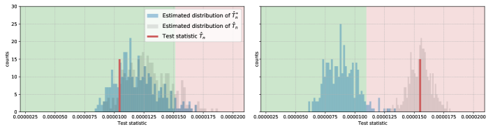
Figure 1: The left (resp. right) figure corresponds to $a=0$, i.e., $\mathcal{H}_{0}$ is valid (resp. $a=0.5$, i.e., $\mathcal{H}_{0}$ is false). Based on a dataset of size $n=1000$, $\hat{T}_{n}$ is computed (red line). Bootstrap statistics $(T^{*}_{n,b})_{b=1,\dots,B}$ $(B=300)$, are used to obtain the distribution of $\hat{T}^{*}_{n}$ (blue). The red area is the rejection region at $5\%$. Independently, $\hat{T}_{n}$ is computed $300$ times to obtain the distribution of in gray.

Cross-validation selection of the number of neighbors.

The number of neighbors $k_{1}$ and $k_{2}$ have a critical effect on the shape of the resulting estimates, and thus on the performance of our test. Indeed, these estimates of the margins $\hat{F}^{(NN)}_{j}(y_{j}|x)$ for $j\in\{1,2\}$ are used in the computation of the test statistic $\hat{T}_{n}$ as well as in the bootstrap procedure to simulate under the null (see Section 2.4). The idea is to assess the performance of each regression model $Y_{1}|X$ and $Y_{2}|X$ and to choose each $k_{1}$ and $k_{2}$ accordingly. We randomly divide the set of observations into $L$ groups of nearly equal size. These groups are denoted by $\{I_{\ell}\}_{\ell=1,\ldots,K}$. Define $\operatorname{MSE}_{j,\ell}(b)=({1}/{|I_{\ell}|})\sum_{i\in I_{\ell}}(Y_{ij}-\hat{g}_{j,k}^{(-\ell)}(X_{i}))^{2}$, where $\hat{g}_{j,k}^{(-\ell)}$ stands for the $k$-nearest neighbors estimate of the regression $Y_{j}|X$ computed on $\{1,\dots,n\}\backslash I_{\ell}$. We choose $k_{j}$ as the minimizer of $({1}/{L})\sum_{\ell=1}^{L}\operatorname{MSE}_{j,\ell}(k)$ over $k$.

The success of the approach in distinguishing $\mathcal{H}_{0}$ from its contrary is illustrated on Figure 1 considering the generic post-nonlinear noise model (when $d=1$) as described in 4.

Remark 3.

Though this example has been carried out using the nearest neighbors estimate of the marginal distributions, other approaches to estimate the marginals can be used to conduct the weighted partial copula test. The only restriction on the employed marginal estimates comes from the bootstrap procedure in which the ability to generate according to each margin is required. This is satisfied for most of the parametric models, e.g., Cox model or Gaussian regression. The broad class of Stone’s weighted regression estimates (Stone, 1977) can also be implemented in our procedure by using multinomial sampling to generate bootstrap samples. This class is important as it includes most of the popular nonparametric estimates: Nadaraya-Watson, nearest neighbors, local linear regression, smoothing splines and Gasser-Muller weights. We refer to (Györfi et al., 2006) and Fan and Gijbels (1996) for an overview of these techniques.

3 Main results

3.1 Consistency of the empirical weighted partial copula and of the test statistics

The results of the section are provided in a general setting in which the estimates of the conditional margins are left unspecified but should satisfy a particular assumption, namely the uniform consistency (UC), given below. We give some examples after the statements of the main results. Let $\mathbb{P}$ denote the probability measure on the underlying probability space associated to the whole sequence $(X_{i},\bm{Y}_{i})_{i=1,2,\ldots}$. In what follows $(r_{n})_{n\geq 1}$ denotes a positive sequence. We write $Z_{n}=O_{\mathbb{P}}(r_{n})$, if $Z_{n}/r_{n}$ is a tight sequence of random variables.

1. For any $j\in\{1,2\}$, we have

   $$\sup_{x\in S_{X},\,y_{j}\in\mathbb{R}}|\hat{F}_{n,j}(y_{j}|x)-F_{j}(y_{j}|x)|=O_{\mathbb{P}}(r_{n})$$

The following result is interested in the uniform consistency of the weighted partial copula process. Its proof is given in the supplementary material.

Theorem 3.

Assume that (UC) holds true and that $w(\cdot)=\tilde{w}(\|\cdot\|)$, where $\tilde{w}:\mathbb{R}_{\geq 0}\mapsto\mathbb{R}$ is of bounded variation. We have, when $n\to\infty$,

$$\sup_{\bm{u}\in[0,1]^{2},\,t\in\mathbb{R}}\left|\hat{W}_{n}(\bm{u},t)-W(\bm{u},t)\right|=O_{\mathbb{P}}(n^{-1/2}+r_{n}).$$

Remark 4.

Theorem 3 is an extension of Theorem 1 in Gijbels et al. (2015). By taking $w=1$ we would recover their result.

Remark 5.

The rate of convergence obtained in Theorem 3 for the partial copula process is as bad as the rate of convergence of the marginal estimate. When the marginal estimates are parametric and therefore attached to a $1/\sqrt{n}$-rate our bound might be sharp. However, when these estimates are nonparametric we conjecture that an improvement in the rate of convergence can be obtained. To illustrate this claim, in the case when $w=1$, $d=1$, and using a smoothed kernel estimate for the margins, Portier and Segers (2018) obtained a rate of convergence of $1/\sqrt{n}$, which is faster than the usual nonparametric convergence rate. Known approaches to achieve such a program relies on the complexity of certain classes generated by conditional quantile estimates. Obtaining guarantees on such complexity would require to focus on particular estimates as the one used in Portier and Segers (2018).

We now provide the following result illustrating the antithetic behavior of $\hat{T}_{n}$ under $\mathcal{H}_{0}$ and its contrary. This cannot be obtained as a corollary of the previous result due to the integration over $t$ which is carried-out over an infinite domain.

Theorem 4.

Assume that (UC) holds true and that $w:\mathbb{R}^{d}\to\mathbb{R}$ is integrable with respect to the Lebesgue measure and with a Fourier transform being non-zero almost everywhere. When $\mathcal{H}_{0}$ is true, we have that $\hat{T}_{n}=O_{\mathbb{P}}(n^{-1}+r_{n}^{2})$ as $n\to\infty$. When $\mathcal{H}_{0}$ is false, there exists $\epsilon>0$ such that $\hat{T}_{n}>\epsilon$ with probability going to $1$ as $n\to\infty$

Remark 6.

The extension to higher dimension $\bm{Y}=(Y_{1},\ldots,Y_{p})$ is straightforward and only represents some minor changes in the proofs of 3 and 4. If the rate $r_{n}$ is not the same for each margin, the final rate obtained is the largest among them.

Remark 7.

Assumption (UC) is satisfied for usual parametric classes $\{F_{\theta}\,:\,\theta\in\Theta\}$. Its validity follows from the consistency of the parameter estimate along with the continuity property $\sup_{x,y}|F_{\theta_{0}}(y|x)-F_{\theta}(y|x)|\to 0$ as soon as $\theta\to\theta_{0}$. Concerning nonparametric methods, (UC) has been the object of several studies for different regression estimates: nearest neighbors (Jiang, 2019), Kaplan-Meier (Dabrowska, 1989) and Nadaraya-Watson (Hansen, 2008). For Nadaraya-Watson weights, (UC) is obtained in (Einmahl and Mason, 2000, Corollary 2) and for a smoothed version of Nadaraya-Watson (UC) is investigated in Portier and Segers (2018). In the next section, we obtain UC for the nearest neighbor estimate described in Section 2.

3.2 Uniform consistency of nearest neighbors marginals estimates

The result presented in this section ensures that (UC) is satisfied for the nearest neighbor estimate of the margins (3). This uniform convergence result, which is new to the best of our knowledge, is introduced independently from the rest of the paper. Let $(X_{i},Y_{i})$, for $i\in\{1,\ldots,n\}$, be independent and identically distributed random vectors, with common distribution equal to the one of $(X,Y)$. The distribution of $X$, $f_{X}$ is supposed to satisfy the following assumption.

1. The density $f_{X}$ is bounded and bounded away from $0$ on $S_{X}=[0,1]^{d}$.

The assumption that $S_{X}$ is the unit cube can be alleviated at the price of some technical assumption given in (Jiang, 2019, Assumption 1). Denote by $F(\cdot|x)$ the conditional distribution of $Y$ given $X=x$. We require the following regularity condition.

1. The function $x\mapsto F(y|x)$ is Lipschitz uniformly in $y\in\mathbb{R}$, i.e.,

   $$\forall(x,x^{\prime})\in S_{X}\times S_{X},\qquad\sup_{y\in\mathbb{R}}|F(y|x)-F(y|x^{\prime})|\leq L\|x-x^{\prime}\|.$$

Theorem 5.

Under (B) and (L), if $k/n\to 0$ and $\log(n)/k\to 0$, we have almost-surely,

$$\sup_{y\in\mathbb{R},\,x\in S_{X}}|\hat{F}^{(NN)}(y|x)-F(y|x)|=O\left(\sqrt{\frac{d}{k}\log(n)}+\left(\frac{k}{n}\right)^{1/d}\right),$$

where $\hat{F}^{(NN)}$ is defined in (3).

Remark 8.

The simple bound given in the previous result is valid in the asymptotic regime $n\to\infty$. It could however be extended to finite sample results at the price of additional technical details.

Remark 9.

The approach employed in the proof relies on controlling the complexity of the nearest neighbors selection mechanism. The main idea is to embed the nearest neighbors selector in a nice class of kernel function having a control complexity. The technique appears to be new in this context and general enough to be extended to estimate of the type

$$k^{-1}{\sum_{i=1}^{n}g(Y_{i})\mathbb{I}_{{\hat{B}}_{k}(x)}(X_{i})},$$

when $g$ is lying on a certain VC class of function. Similar quantities, using a kernel smoothing approach, have been considered in (Einmahl and Mason, 2000).

Remark 10.

Optimal rates of convergence (for Lipschitz functions) are achieved when selecting $k=n^{2/(d+2)}$ as it gives a uniform error of order $n^{-1/(d+2)}$ (Stone, 1982).

4 Numerical experiments

In this section, we apply the proposed copula test to synthetic and real data to evaluate its performance based on the nominal level and the power of the test. The weighted partial copula test is put to work with two different margins estimates. As a first approach, we consider the following parametric estimate of the conditional margins:

$$\hat{F}_{n,j}^{(LR)}(y|x)=\Phi_{\left(x^{\top}\hat{\beta}_{j},\hat{\sigma}\right)}(y),\qquad(y\in{\mathbb{R}}),$$ (4)

where $\Phi_{(m,\sigma)}$ denotes the c.d.f. of a normal distribution of mean $m$ and mean $m$ and variance $\sigma^{2}$. This estimate will be referred to as the linear regression (LR) estimate because $\hat{\beta}_{j}$ is estimated by minimizing the sum of squares in a linear model ($\hat{\sigma}^{2}$ is chosen as the variance of the estimated residuals). In fact, $\hat{F}_{n,j}^{(LR)}$ is the classical Gaussian maximum likelihood estimator of the margin $F_{j}$. Representing a more flexible approach, we use the nearest neighbors (NN) estimate given in (3) for the margins. For both approach, the function $w$ is a Gaussian kernel given by $w(t)=\exp(-\|t\|^{2})$ and $B=200$ bootstrap realizations.

We compare our approach with the KCI-test Zhang et al. (2011) presented in the related literature section. Since the level $\alpha$ is hard to set for the CCI-test of Sen et al. (2017), this approach will only be considered when the proportions of correct decision will be computed (see Figure 3(a)). The Python source code used to run our test is available in a supplementary material file.

In the whole numerical study, we set $\alpha=5\%$ as the desired type-I error rate. All results are averaged over $300$ trials.

4.1 Linear Model

Consider the joint distribution given by $Y_{1}=X^{T}\beta_{1}+\epsilon_{1},Y_{2}=X^{T}\beta_{2}+\epsilon_{2},$ where $X\sim\mathcal{N}(0,\mathsf{I}_{d}),\beta_{1}\text{and }\beta_{2}$ are two constant vectors of $[0,1]^{d},$ and $\epsilon_{1},\epsilon_{2}$ are two standard Gaussian variables with $\operatorname{Cov}(\epsilon_{1},\epsilon_{2})=a$. When $a=0$, $\mathcal{H}_{0}$ is true. It is false when $a>0$. We examine the effect of the constant $a>0$, and the size of the dataset $n$ on the type-II error rate. We also examine the type-I errors when the dimension of the variable $X$ increases, in a setting where the null hypothesis $\mathcal{H}_{0}$ holds.

Figure 2 shows the attractive performance of our test compared to the KCI-test. Notably, we can see that in high dimensions, our test is more accurate with respect to the level set $\alpha$ than the KCI-test.

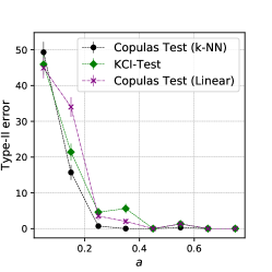
(a) $n=1000,$ various $a$, $d=1$

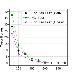
(b) various $n$, $a=0.3$, $d=1$

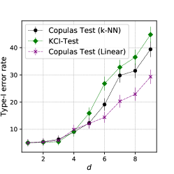
(c) $a=0$, $n=1000$, various $d$

Figure 2: Simulation results for the linear model. Figures 2(a), 2(b) show the probability of acceptance (i.e. the type II error rate), plotted against the constant $a$ and $n$. Figure 2(c) shows the probability of rejection (type I error) against $d$. The plots show the average probabilities with standard error bars.

4.2 Disturbed Linear Model

In this section, we consider a slight perturbation appearing in the linear model of Section 4.1 as follows: $Y_{1}=X^{T}\beta_{1}+\epsilon_{1}$, $Y_{2}=c\|X\|+X^{T}\beta_{2}+\epsilon_{2},$ where $X\sim\mathcal{N}(0,\mathsf{I}_{d}),\beta_{1}\text{and }\beta_{2}$ are two constant vectors of $[0,1]^{d},$ $c\geq 0$, and $\epsilon_{1},\epsilon_{2}$ are two centered Gaussian variables with $\operatorname{Cov}(\epsilon_{1},\epsilon_{2})=a$. We set $a=0.2$ and we examine the effect of the constant $c>0$, and the dimension $d$ of $X$ on the type-II error rate. We also examine the type-I errors when $d$ increases, in a setting where the null hypothesis $\mathcal{H}_{0}$ holds.

4.3 Causality Discovery

Hereinafter we consider a particular type of DAG called latent cause model. To draw samples from the alternative hypothesis, we break the conditional independence by adding an edge between the nodes $Y_{1}$ and $Y_{2}$. For the ”Latent cause“ model of interest we have $X\sim\mathcal{N}(0,1),$ $Y_{1}|X\sim\mathcal{N}(X,1),$ and $Y_{2}|X,Y_{1}\sim\mathcal{N}(X+aY_{1},1)$. It is easy to verify that $\mathcal{H}_{0}$ is true when $a=0$, and false otherwise. It can be seen in Figure 3 that for large sample size $n$, our test outperforms the ones in competition. Furthermore, our test is slightly more powerful than the KCI-test across a range of values of $a$ but overall shows fairly similar performance.

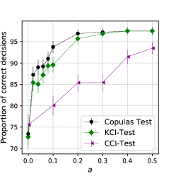
(a) $n=1500$, various $a$

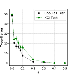
(b) $n=1500$, various $a$

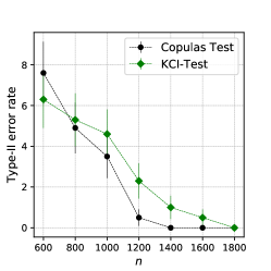
(c) $a=0.3$, various $n$

Figure 3: Simulation results for the causal inference datasets.

4.4 Post-Nonlinear Noise

We apply the proposed test on the post-nonlinear noise model. We first examine the effect of the constant $a>0$ on the probability of type-I and type-II error of our test. The results are shown in Figure 4. As expected, larger values of $a$ yields lower type-II error probabilities. For every value $a$, we observe that the type-I error probability is close to $\alpha$. The performances of the tests are also compared when the sample size $n$ changes. The role of $n$ is critical and the results are shown in Figure 5. We note that the type-I error probability is again close to $\alpha$ and that the type-II quickly vanishes when $n$ increases. In this experiment, the proposed procedure outperforms the KCI-test.

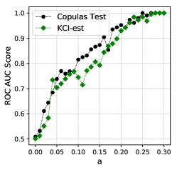
(a) $n=500,$ various $a$ and $d=1$

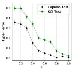
(b) $n=500,$ various $a$ and $d=1$

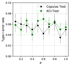
(c) $n=500,$ various $a$ and $d=1$

Figure 4: Simulation results for the post-nonlinear noise model. Figures 4(a), 4(b) and 4(c), show respectively the ROC AUC score, the probability of acceptance (i.e. the type II error rate), and the type I error rate plotted against the constant $a$ with standard error bars.

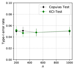
(a) $a=0.5$, various $n$, $d=1$

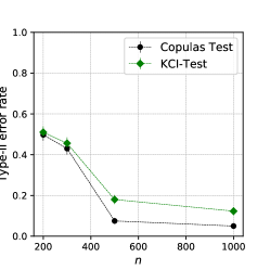
(b) $a=0.5$, various $n$, $d=1$

Figure 5: The probability of type-I (5(b)) and type-II (5(b)).

4.5 Classification of age groups using functional connectivity

In this paragraph, we apply our test in a practical setting, using the movie watching based brain development dataset Richardson et al. (2018) obtained from the OpenNeuro database. The dataset consists in $50$ patients ($10$ adults and $40$ children). The fMRI data consists in measuring the brain activity in 39 Region of Interest (ROI). For every patient, $168$ measurements are provided for each ROI. We denote for $j\in\{1,\dots,39\}$ by $X_{j}$ the variable that represents the $j^{th}$ region signal value. Given two ROI $j$ and $j^{\prime}$, we seek to test the null hypothesis that $X_{j}$ and $X_{j^{\prime}}$ are conditionally independent given $\mathbf{X}_{\backslash\{j,j^{\prime}\}}$. The decisions given by our test allow us to obtain a map of connections between all the ROI, called connectome, given in Figure 6. In this figure, a line is drawn between two ROI whenever our test rejects the null for these two ROI. Here, due to the high dimension of the conditional variable, the margins are no longer estimated using a Gaussian kernel as in Section 2.5, but using a $k$-nearest neighbours approach. For a given $x$, the mapping $\hat{F}_{n,j}(y|x)$ is estimated for every $y\in\mathbb{R}$ as the proportion of samples $i$ amongst the $k$-nearest nearest neighbours of $x$ which satisfy $Y_{ij}\leq y$. The integer $k$ is select by cross-validation.

As a sanity check, our connectome is used as an input feature of a classifier (Linear Support Vector Classifier (SVC)) in order to distinguish children from adults. We estimate the classification accuracy of our classifier using $k$-fold. The obtained accuracy is 97.4$\%$. This result outperforms the standard correlation method (91.3$\%$) and is close to the so-called tangent method (98.9$\%$) which is known to be fitted for this task Dadi et al. (2019).

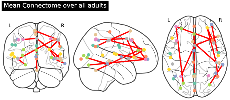
Figure 6: Mean connectome provided by our test over all adults.

Conclusion

In this work, we have developed test of conditional independence between $Y_{1}$ and $Y_{2}$ given $X$ based on weighted partial copulas. First, under general conditions, the consistency of the weighted partial copula process has been established. We have shown that, empirically, our proposed test shows better performance, in terms of power, than recent state-of-the-art conditional independence tests such as the one based on a kernel embedding.

Appendix A Proofs of the basic lemmas of Section 2

A.1 Proof of Lemma 1

The “only if” part is obvious. Suppose that the function $W=0$ and let $\bm{u}\in[0,1]^{2}$. Define $g(x)=C(\bm{u}\mid x)-u_{1}u_{2})f_{X}(x)$. We have $(g\star w)=0$, a.e. on $\mathbb{R}^{d}$, where $\star$ stands for the standard convolution product with respect to the Lebesgue measure. Applying the Fourier transform gives that $\mathcal{F}(g)\mathcal{F}(w)=0$ which, by assumption, yields $\mathcal{F}(g)=0$. By the Fourier inversion theorem we obtain that $g=0$ a.e. on $\mathbb{R}^{d}$. That is for any $\bm{u}\in[0,1]^{2}$ and any $x\in S_{X}$, $C(\bm{u}\mid x)=u_{1}u_{2}$.

∎

A.2 Proof of Lemma 2

Write

$$\hat{T}_{n} =n^{-2}\sum_{1\leq i,j\leq n}\int_{[0,1]^{2}}\xi_{i}(\bm{u})\xi_{j}(\bm{u})\,\mathrm{d}\bm{u}\int_{\mathbb{R}^{d}}\omega(t-X_{i})\omega(t-X_{j})\,\mathrm{d}t,$$

where $\xi_{k}(\bm{u})=\mathds{1}_{\{\hat{G}_{k1}\,<\,u_{1}\}}\mathds{1}_{\{\hat{G}_{k2}\,<\,u_{2}\}}-u_{1}u_{2}$. It remains to compute the function $M$. Using the notation $\hat{\bm{G}}_{i}$, we have

$$\int_{[0,1]^{2}}\xi_{i}(\bm{u})\xi_{j}(\bm{u})\,\mathrm{d}\bm{u}= \int_{[0,1]^{2}}\mathds{1}_{\{\hat{G}_{i1}\,<\,u_{1}\}}\mathds{1}_{\{\hat{G}_{i2}\,<\,u_{2}\}}\mathds{1}_{\{\hat{G}_{j1}\,<\,u_{1}\}}\mathds{1}_{\{\hat{G}_{j2}\,<\,u_{2}\}}\mathrm{d}\bm{u}$$

$$-\int_{[0,1]^{2}}\mathds{1}_{\{\hat{G}_{i1}\,<\,u_{1}\}}\mathds{1}_{\{\hat{G}_{i2}\,<\,u_{2}\}}u_{1}u_{2}\mathrm{d}\bm{u}$$

$$-\int_{[0,1]^{2}}\mathds{1}_{\{\hat{G}_{j1}\,<\,u_{1}\}}\mathds{1}_{\{\hat{G}_{j2}\,<\,u_{2}\}}u_{1}u_{2}\mathrm{d}\bm{u}+\int_{[0,1]^{2}}(u_{1}u_{2})^{2}\mathrm{d}\bm{u}.$$

First, let compute the first term of the right hand side. Let notice that the value of the integrand is 1 if $u_{1}>\hat{G}_{i1}\vee\hat{G}_{j1}$ and $u_{2}>\hat{G}_{u2}\vee\hat{G}_{j2}$ and $0$ otherwise. Thus we obtain for this term:

$$\int_{[0,1]^{2}} \mathds{1}_{u_{1}>\hat{G}_{i1}\vee\hat{G}_{j1}}\mathds{1}_{u_{2}>\hat{G}_{i2}\vee\hat{G}_{j2}}\mathrm{d}\bm{u}=\left(1-\hat{G}_{i1}\vee\hat{G}_{j1}\right)\left(1-\hat{G}_{i2}\vee\hat{G}_{j2}\right).$$ (5)

Now let derive the second integral term of the right hand side, the third term will follow directly.

$$\int_{[0,1]^{2}}\mathds{1}_{\{\hat{G}_{i1}\,<\,u_{1}\}}\mathds{1}_{\{\hat{G}_{i2}\,<\,u_{2}\}}u_{1}u_{2}\mathrm{d}\bm{u} =\int_{[0,1]}\mathds{1}_{\{\hat{G}_{i1}\,<\,u_{1}\}}u_{1}\mathrm{d}u_{1}\int_{[0,1]}\mathds{1}_{\{\hat{G}_{i2}\,<\,u_{2}\}}u_{2}\mathrm{d}u_{2}$$

$$=\frac{1}{4}\left(1-\hat{G}_{i1}^{2}\right)\left(1-\hat{G}_{i2}^{2}\right).$$ (6)

By combining (5) and (A.2) we obtain the desired result. ∎

Appendix B Proof of Theorem 3

The proof is inspired from the proof Theorem 1 in Gijbels et al. (2015).

Notation.

We use notation from empirical process theory. Let $P_{n}=n^{-1}\sum_{i=1}^{n}\delta_{(X_{i},\bm{Y}_{i})}$ denote the empirical measure. For a function $f$ and a probability measure $Q$, write $Qf=\int f\,\mathrm{d}Q$. The empirical process is

$$\mathbb{G}_{n}=n^{1/2}(P_{n}-P).$$

For any pair of cumulative distribution functions $F_{1}$ and $F_{2}$ on $\mathbb{R}$, put $\bm{F}(\bm{y})=(F_{1}(y_{1}),F_{2}(y_{2}))$ for $\bm{y}=(y_{1},y_{2})\in\mathbb{R}^{2}$ and $\bm{F}^{-}(\bm{u})=(F_{1}^{-}(u_{1}),F_{2}^{-}(u_{2}))$ for $\bm{u}=(u_{1},u_{2})\in[0,1]^{2}$.

Preliminary results.

Fact 1.

$$\sup_{u_{j}\in[0,1]}|\hat{G}_{n,j}(u_{j})-u_{j}|=O_{\mathbb{P}}(r_{n}+n^{-1/2}).$$

Proof.

With probability at least $1-\epsilon/2$,

$$\sup_{u_{j}\in[0,1],\,x\in S_{X}}|\hat{F}_{n,j}(u_{j}|x)-F(u_{j}|x)|\leq Mr_{n}.$$

Moreover, from Donsker’s theorem, we have with probability $1-\epsilon/2$

$$\sup_{u_{j}\in\mathbb{R}}(P_{n}-P)\{\mathds{1}_{\{{F}_{j}\,\leq\,u_{j}\}}\}\leq Mn^{-1/2}.$$

As a consequence, we have with probability $1-\epsilon$,

$$\hat{G}_{n,j}(u_{j}) =P_{n}\mathds{1}_{\{\hat{{F}}_{n,j}\,\leq\,u_{j}\}}$$

$$\leq P_{n}\mathds{1}_{\{{F}_{j}\,\leq\,u_{j}+Mr_{n}\}}$$

$$\leq P\mathds{1}_{\{{F}_{j}\,\leq\,u_{j}+Mr_{n}\}}+Mn^{-1/2}.$$

Using that $P\mathds{1}_{\{{F}_{j}\,\leq\,u_{j}+Mr_{n}\}}=u_{j}+Mr_{n}$, we have shown that

$$\hat{G}_{n,j}(u_{j})-u_{j}\leq M(r_{n}+n^{-1/2})$$

The lower bound $\hat{G}_{n,j}(u_{j})-u_{j}\geq-M(r_{n}+n^{-1/2})$ can be obtained in the same way. ∎

Fact 2.

$$\sup_{u_{j}\in[0,1],\,x\in S_{X}}|\hat{G}_{n,j}(\hat{{F}}_{n,j}(u_{j}|x))-F(u_{j}|x)|=O_{\mathbb{P}}(r_{n}+n^{-1/2}).$$

Proof.

Using the triangle inequality and Fact 1 leads to the result. ∎

Fact 3.

$$\sup_{\bm{u}\in[0,1]^{2},\,t\in\mathbb{R}}|(P_{n}-P)\left\{w_{t}\mathds{1}_{\{\bm{F}\,\leq\,\bm{u}\}}\right\}|=O_{\mathbb{P}}(n^{-1/2}).$$

Proof.

Since $\tilde{w}$ is of bounded variation, the function class $\{x\mapsto w_{t}(x)\,:\,t\in\mathbb{R}\}$ is Euclidean (or VC) with constant envelop $C_{w}=\sup_{x\in\mathbb{R}}|w(x)|$ (Nolan and Pollard, 1987, Lemma 22, (i)), i.e., the covering numbers are polynomials. Moreover, the class of indicator functions is also Euclidean (van der Vaart and Wellner, 1996, Example 2.5.4). This implies that both classes have finite entropy integrals and therefore are Donsker (van der Vaart and Wellner, 1996, Chapter 2.1, equation (2.1.7)). Using the preservation of the Donsker property through products and sums (van der Vaart and Wellner, 1996, Example 2.10.7 and 2.10.8), the class $\{(\bm{y},x)\mapsto w_{t}(x)\mathds{1}_{\{\bm{F}(\bm{y}|x)\leq\bm{u}\}}\,:\,t\in\mathbb{R},\,\bm{u}\in[0,1]^{2}\}$ is Donsker. As a result, the process $\{\mathbb{G}_{n}\{w_{t}\mathds{1}_{\{\bm{F}\,\leq\,\bm{u}\}}\}_{\bm{u}\in[0,1]^{2},\,t\in\mathbb{R}}$ converges weakly to a tight Gaussian process in $\ell^{\infty}([0,1]^{2}\times\mathbb{R})$. ∎

End of the proof.

We need to show that $W_{n}(\bm{u},t)-W(\bm{u},t)=O_{\mathbb{P}}(r_{n}+n^{-1/2})$. Let $\epsilon>0$. From Fact 2 and Fact 3, we have with probability $1-\epsilon$,

$$W_{n}(\bm{u},t) =P_{n}\left\{w_{t}(\mathds{1}_{\{\hat{\bm{F}}_{n}\,\leq\,\hat{\bm{G}}^{-}_{n}(\bm{u})\}}\right\}$$

$$=P_{n}\left\{w_{t}(\mathds{1}_{\{\hat{\bm{G}}_{n}\hat{\bm{F}}_{n}\,<\,\bm{u}+n^{-1}\}}\right\}$$

$$\leq P_{n}\left\{w_{t}\mathds{1}_{\{{\bm{F}}\,\leq\,\bm{u}+a_{n}\}}\right\}$$

$$=P\left\{w_{t}(\mathds{1}_{\{{\bm{F}}\,\leq\,\bm{u}+a_{n})\}}\right\}+Mn^{-1/2}$$

$$=W(\bm{u},t)+L_{n}+Mn^{-1/2}$$

with

$$L_{n}=P\left\{w_{t}(\mathds{1}_{\{{\bm{F}}\,\leq\,\bm{u}+a_{n}\}}-\mathds{1}_{\{{\bm{F}}\,\leq\,\bm{u}\}})\right\}$$

$$a_{n}=n^{-1}+M(r_{n}+n^{-1/2})$$

for some $M>0$. Now, because of the $1$-Lipschitz properties of copulas (Durante and Sempi, 2015, Theorem 1.5.1), we have

$$L_{n} =\int w_{t}(x)\left\{C(\bm{u}+a_{n}\mid x)-C(\bm{u}\mid x)\right\}\,f_{X}(x)\,\mathrm{d}x\leq 2C_{w}a_{n}.$$

Consequently, we have shown that with probability $1-\epsilon$,

$$P_{n}\left\{w_{t}\mathds{1}_{\{\hat{\bm{F}}_{n}\,\leq\,\hat{\bm{G}}^{-}_{n}(\bm{u})\}}\right\}\leq W(\bm{u},t)+2C_{w}a_{n}+Mn^{-1/2}.$$

Proceeding the same way, we obtain $P_{n}\left\{w_{t}\mathds{1}_{\{\hat{\bm{F}}_{n}\,\leq\,\hat{\bm{G}}^{-}_{n}(\bm{u})\}}\right\}\geq W(\bm{u},t)-2C_{w}a_{n}-Mn^{-1/2}$ which implies the desired the result.

Appendix C Proof of Theorem 4

In virtue of Lemma 1, it suffices to show that

$$\int(W_{n}(\bm{u},t)-W(\bm{u},t))^{2}\mathrm{d}t=O_{\mathbb{P}}(r_{n}+n^{-1}).$$

We start recalling that $\tilde{W}_{n}(\bm{u}-a_{n},t)\leq W_{n}(\bm{u},t)\leq\tilde{W}_{n}(\bm{u}+a_{n},t)$ with

$$\tilde{W}_{n}(\bm{u},t)=P_{n}\left\{w_{t}\mathds{1}_{\{{\bm{F}}\,\leq\,\bm{u}\}}\right\},$$

as established in the proof of Theorem 3. As a consequence

$$\int(W_{n}(\bm{u},t)-W(\bm{u},t))^{2}\mathrm{d}t$$

$$\leq\max_{z\in[-1,1]}\int(\tilde{W}_{n}(\bm{u}+za_{n},t)-W(\bm{u},t))^{2}\mathrm{d}t$$

$$\leq 2\max_{z\in[-1,1]}\left(\int(\tilde{W}_{n}(\bm{u}+za_{n},t)-W(\bm{u}+za_{n},t))^{2}\mathrm{d}t+\int(W(\bm{u}+za_{n},t)-W(\bm{u},t))^{2}\mathrm{d}t\right)$$

$$\leq 2\sup_{\bm{u}\in\mathbb{R}^{2}}\int(\tilde{W}_{n}(\bm{u},t)-\tilde{W}_{n}(\bm{u},t))^{2}\mathrm{d}t+2\max_{z\in[-1,1]}\int(W(\bm{u}+za_{n},t)-W(\bm{u},t))^{2}\mathrm{d}t$$

Each terms are handled separately. One has that

$$\int(\tilde{W}_{n}(\bm{u},t)-\tilde{W}_{n}(\bm{u},t))^{2}\mathrm{d}t$$

$$=2n^{-2}\sum_{i<j}\int(f_{i}(\bm{u},t)-Ef_{i}(\bm{u},t))(f_{j}(\bm{u},t)-Ef_{j}(\bm{u},t))\mathrm{d}t+n^{-2}\sum_{i=1}^{n}\int(f_{i}(\bm{u},t)-Ef_{i}(\bm{u},t))^{2}\mathrm{d}t$$

$$\leq n^{-2}\sum_{i<j}\int(f_{i}(\bm{u},t)-Ef_{i}(\bm{u},t))(f_{j}(\bm{u},t)-Ef_{j}(\bm{u},t))\mathrm{d}t+2n^{-1}f_{\infty}$$

with $f_{i}(\bm{u},t)=w_{t}(X_{i})\mathds{1}_{\{{\bm{F}}(\bm{Y}_{i}|X_{i})\,\leq\,\bm{u}\}}$ and $f_{\infty}=\sup_{x\in S_{X}}\int w_{t}(x)^{2}\mathrm{d}t\leq C_{w}\|w\|_{1}$. We now recognize a degenerate $U$-statistics in the above right-hand side term. Indeed, using Fubini’s theorem,

$$\int(f_{i}(\bm{u},t)-Ef_{i}(\bm{u},t))(f_{j}(\bm{u},t)-Ef_{j}(\bm{u},t))\,\mathrm{d}t$$

$$=\int(g_{i,j}(\bm{u},t)-E[g_{i,j}(\bm{u},t)|i]-E[g_{i,j}(\bm{u},t)|j]+E[g_{i,j}(\bm{u},t)])\,\mathrm{d}t$$

$$=h_{i,j}(\bm{u})-E[h_{i,j}(\bm{u})|i]-E[h_{i,j}(\bm{u})|j]+E[h_{i,j}(\bm{u})]$$

with

$$g_{i,j}(\bm{u},t)=w_{t}(X_{i})w_{t}(X_{j})\mathds{1}_{\{{\bm{F}}(\bm{Y}_{i}|X_{i})\,\leq\,\bm{u}\}}\mathds{1}_{\{{\bm{F}}(\bm{Y}_{j}|X_{j})\,\leq\,\bm{u}\}}$$

$$h_{i,j}(\bm{u})=w^{\star}(X_{i}-X_{j})\mathds{1}_{\{{\bm{F}}(\bm{Y}_{i}|X_{i})\,\leq\,\bm{u}\}}.$$

As the function class $\{h_{i,j}\,:\,\bm{u}\in\mathbb{R}^{2}\}$ is of VC type (see Corollary 21 in Nolan and Pollard (1987)), we are in position to apply Theorem 2 in Major (2006), leading to

$$\sup_{\bm{u}\in\mathbb{R}^{2}}\left|\sum_{i<j}\int(f_{i}(\bm{u},t)-Ef_{i}(\bm{u},t))(f_{j}(\bm{u},t)-Ef_{j}(\bm{u},t))\mathrm{d}t\right|=O_{\mathbb{P}}(n).$$

As a consequence $\sup_{\bm{u}\in\mathbb{R}^{2}}\int(\tilde{W}_{n}(\bm{u},t)-\tilde{W}_{n}(\bm{u},t))^{2}\mathrm{d}t=O_{\mathbb{P}}(n^{-1})$. Now we bound the remaining term, $\max_{z\in[-1,1]}\int(W(\bm{u}+za_{n},t)-W(\bm{u},t))^{2}\mathrm{d}t$. As in the proof of Theorem 3, we use the Lipschitz property of copulas. It gives

$$|W(\bm{u}+za_{n},t)-W(\bm{u},t)|\leq 2a_{n}\int w_{t}(x)f_{X}(x)\,\mathrm{d}x.$$

Then applying Jensen’s inequality gives that

$$\int|W(\bm{u}+za_{n},t)-W(\bm{u},t)|^{2}\,\mathrm{d}t \leq 4a_{n}^{2}\int\int w_{t}(x)^{2}\,\mathrm{d}tf_{X}(x)\,\mathrm{d}x\leq 4C_{w}\|w\|_{1}a_{n}^{2}.$$

Appendix D Proof of Theorem 5

Auxiliary results.

The following result is Theorem 15 in Chaudhuri and Dasgupta (2010) when applied to the collection of balls

$$\mathcal{B}=\{B(x,\tau)\,:\,x\in[0,1]^{d}\,\tau>0\},$$

where $B(x,\tau)$ is the ball with center $x$ and radius $\tau$.

Theorem 6.

For any $\delta>0$ and $n\geq 1$, with probability at least $1-\delta$:

$$-\beta_{n}^{2}+\beta_{n}\sqrt{P(B)}\leq P(B)-P_{n}(B)\leq\beta_{n}\sqrt{P(B)},\qquad\forall B\in\mathcal{B},$$

with $\beta_{n}=\sqrt{c_{1}(d/n)\log(c_{2}n/\delta)}$, $c_{1}>0$ and $c_{2}>0$ universal constants.

Let $(S,\mathcal{S})$ be a measurable space. Given a probability measure $Q$ on $\mathcal{S}$, define the metric space $L_{2}(Q)$ of $Q$-square-integrable functions, i.e.,

$$L_{2}(Q)=\{g:S\mapsto\mathbb{R}\,:\,\|g\|_{L_{2}(Q)}<\infty\},$$

where $\|g\|_{L_{2}(Q)}^{2}=\int g^{2}dQ$. Given $\mathcal{G}\subset L_{2}(Q)$, the $\epsilon$-covering number $\mathcal{N}(\mathcal{G},L_{2}(Q),\epsilon)$ is the smallest number of open balls of radius $\epsilon>0$ required to cover $\mathcal{G}$. For the definition of VC classes, we follow Giné and Guillou (2002). Note that similar classes (sometimes with different names) have been defined earlier in the literature (Nolan and Pollard, 1987). Next we call an envelop for $\mathcal{G}$ any function $G:S\mapsto\mathbb{R}$ that satisfies $|g(x)|\leq G(x)$ for all $x\in S$.

Definition 1 (VC-class).

A class $\mathcal{G}$ of real functions on a measurable space $(S,\mathcal{S})$ is called a VC-class of parameters $(v,A)\in(0,\infty)^{2}$ with respect to the envelope $G$ if for any $0<\epsilon<1$ and any probability measure $Q$ on $(S,\mathcal{S})$, we have

$$\mathcal{N}\left(\mathcal{G},L_{2}(Q),\epsilon\|G\|_{L_{2}(Q)}\right)\leq(A/\epsilon)^{v}.$$

The following concentration result is tailored to VC classes of functions. The result stated in Theorem 7 below is a consequence of the work in Giné and Guillou (2001) which is based on Talagrand (1996). The next formulation is slightly different in that the role played by the VC constants ($v$ and $A$ below) is quantified.

Theorem 7.

Let $\mathcal{G}$ be a VC class of functions with parameters $(v,A)$ and uniform envelop $U>0$. Let $\sigma$ be such that $\sigma^{2}\geq\sup_{g\in\mathcal{G}}\sigma^{2}_{P}(g)$ and $\sigma\geq U$. Let $n\geq 1$ and $\delta\in(0,1)$ be such that

$$\sqrt{n}\sigma\geq c_{1}\sqrt{U^{2}v\log(AU/(\sigma\delta))},$$

then, we have with probability $1-\delta$,

$$\sup_{f\in\mathcal{G}}\left|(P_{n}-P)(g)\right|\leq c_{2}\sqrt{\frac{\sigma^{2}v\log(AU/(\sigma\delta))}{n}},$$

where $c_{1}$ and $c_{2}$ are positive constants.

Preliminary results.

Define $b>0$ and $U>0$ such that $b<f_{X}<U$ and set

$$\hat{\tau}_{n,k}(x){=}\inf\{\tau\geq 0\,:\,\sum_{i=1}^{n}\mathds{1}_{{B}(x,\tau)}(X_{i})\geq k\},$$

$$\overline{\tau}_{n,k}=\left(\frac{2k}{nb_{f}V_{d}}\right)^{1/d},$$

$$\underline{\tau}_{n,k}=\left(\frac{k}{2nU_{f}V_{d}}\right)^{1/d},$$

where $V_{d}$ is the volume of the unit ball in $\mathbb{R}^{d}$ and $0<b_{f}\leq U_{f}$ are constant factors that are defined right after. Note that $\hat{B}_{k}(x)={B}(x,\hat{\tau}_{n,k}(x))$. The next lemma is the starting point of our proof. As in Jiang (2019), it will be useful to control the size of the nearest neighbors balls.

Lemma 8.

Suppose that (B) is fulfilled and that $\log(n)/k\to 0$. We have with probability $1$: there exists $N\geq 1$ such that for all $n\geq N$,

$$\sup_{x\in[0,1]^{d}}\sum_{i=1}^{n}\mathds{1}_{B(x,\underline{\tau}_{n,k})}(X_{i})\leq k\leq\inf_{x\in[0,1]^{d}}\sum_{i=1}^{n}\mathds{1}_{B(x,\overline{\tau}_{n,k})}(X_{i}).$$

Proof.

Using (B) yields

$$P(X\in{B}(x,\overline{\tau}_{n,k}))=\int_{{B}(x,\overline{\tau}_{n,k})\cap[0,1]^{d}}f_{X}\geq b_{f}\lambda({B}(x,\overline{\tau}_{n,k}))=b_{f}V_{d}\overline{\tau}_{n,k}^{d}=2k/n,$$

for some constant factor $b_{f}>0$. Similarly, we have

$$P(X\in{B}(x,\underline{\tau}_{n,k}))\leq k/(2n)$$

Applying Lemma 6 with $\delta=n^{-2}$ and using that $\log(n)/k\to 0$ and taking $n$ large enough, we obtain that with probability at least $n^{-2}$, for all $x\in[0,1]^{d}$,

$$n^{-1}\sum_{i=1}^{n}\mathds{1}_{B(x,\overline{\tau}_{n,k})}(X_{i}) \geq\frac{1}{2}P(B(x,\overline{\tau}_{n,k})\geq k/n.$$

As a consequence of the Borel-Cantelli lemma, we obtain that with probability $1$, for $n$ large enough,

$$\inf_{x\in[0,1]^{d}}\sum_{i=1}^{n}\mathds{1}_{B(x,\overline{\tau}_{n,k})}(X_{i})\geq k.$$

The upper bound is obtained similarly. ∎

Lemma 9.

Suppose that (B) is fulfilled and that $\log(n)/k\to 0$. We have with probability $1$: there exists $N\geq 1$ such that for all $n\geq N$,

$$\underline{\tau}_{n,k}\leq\inf_{x\in[0,1]^{d}}\hat{\tau}_{n,k}(x)\leq\sup_{x\in[0,1]^{d}}\hat{\tau}_{n,k}(x)\leq\overline{\tau}_{n,k}$$

Proof.

By definition of $\hat{\tau}_{n,k}(x)$, on the event that $\sum_{i=1}^{n}\mathds{1}_{B(x,\overline{\tau}_{n,k})}(X_{i})\geq k$ it holds that $\hat{\tau}_{n,k}(x)\leq\overline{\tau}_{n,k}$. ∎

End of the proof.

We rely on the classical bias-variance decomposition

$$\hat{F}^{(NN)}(y|x)-F(y|x)=\sum_{i=1}^{n}w_{i}(\mathbb{I}_{\{Y_{i}\leq y\}}-F(y|X_{i}))+\sum_{i=1}^{n}w_{i}(F(y|X_{i})-F(y|x)),$$

where $w_{i}=k^{-1}\mathds{1}_{\{\hat{B}_{k}(x)\}}(X_{i})$. We have

$$\left|\sum_{i=1}^{n}w_{i}(F(Y_{i}|X_{i})-F(y|x))\right| \leq\sup_{x^{\prime}\in\hat{B}_{n,k}(x)}|F(y|x^{\prime})-F(y|x)|\leq L\hat{\tau}_{n,k}(x).$$

Applying Lemma 9 we obtain that, with probability $1$, for $n$ is large enough,

$$\left|\sum_{i=1}^{n}w_{i}(F(Y_{i}|X_{i})-F(y|x))\right|\leq L\overline{\tau}_{n,k}.$$

Besides, we write

$$\sum_{i=1}^{n}w_{i}(\mathds{1}_{\{Y_{i}\leq y\}}-F(y|X_{i}))=k^{-1}\sum_{i=1}^{n}(\mathds{1}_{\{Y_{i}\leq y\}}-F(y|X_{i}))\mathds{1}_{{\hat{B}}_{k}(x)}(X_{i})$$

Due to Lemma 9, we have for $n$ large enough,

$$\sup_{y\in\mathbb{R},\,x\in[0,1]^{d}}\left|\sum_{i=1}^{n}(\mathds{1}_{\{Y_{i}\leq y\}}-F(y|X_{i}))\mathds{1}_{{\hat{B}}_{k}(x)}(X_{i})\right|$$

$$\leq\sup_{y\in\mathbb{R},\,B\in B(\overline{\tau}_{n,k})}\left|\sum_{i=1}^{n}(\mathds{1}_{\{Y_{i}\leq y\}}-F(y|X_{i}))\mathds{1}_{B}(X_{i})\right|,$$

where $\mathcal{B}(\overline{\tau}_{n,k})$ is the set of all balls having radius smaller than $\overline{\tau}_{n,k}$. Hence, the class of interest is

$$\mathcal{G}=\{(y,x)\mapsto(\mathds{1}_{\{Y_{i}\leq y\}}-F(y|X_{i}))\mathbb{I}_{B}(X_{i})\,:\,y\in\mathbb{R},\,B\in\mathcal{B}(\overline{\tau}_{n,k})\}.$$

The class of cells $\mathds{1}_{\{Y_{i}\leq y\}}$, $y\in\mathbb{R}$ is VC with parameter $v$ independent of the dimension (van der Vaart and Wellner, 1996). The class of balls $\mathcal{B}$ is VC with $v\propto d$ (Wenocur and Dudley, 1981). It follows that their product is of VC-type with dimension proportional to $d$. Noting that $E[\mathds{1}_{\{Y_{1}\leq y\}}\mathbb{I}_{B}(X_{1})|X_{1}]=F(y|X_{1})\mathbb{I}_{B}(X_{1})$ we can use Lemma 20 in Nolan and Pollard (1987) to prove that $F(y|X_{1})\mathbb{I}_{B}(X_{1})$ is VC with $v\propto d$. Finally, an appeal to Lemma 16 Nolan and Pollard (1987) implies that the class $\mathcal{G}$ is VC with constant $v\propto d$ and envelop $U=2$. Consequently, we can apply Theorem 7 with $U=2$. Moreover

$$\sup_{y\in\mathbb{R},\,B\in\mathcal{B}(\overline{\tau}_{n,k})}E[(\mathbb{I}_{\{Y_{1}\leq y\}}-F(y|X_{1}))^{2}\mathbb{I}_{B(x,\tau)}(X_{1})^{2}] \leq\sup_{B\in\mathcal{B}(\overline{\tau}_{n,k})}E[\mathbb{I}_{B}(X_{1})].$$

In a similar way as in the proof of Lemma 8, we find

$$P(X\in{B}(x,\overline{\tau}_{n,k}))\leq U_{f}V_{d}\overline{\tau}_{n,k}^{d}=(U_{f}/b_{f})(2k/n).$$

Hence we can take $\sigma^{2}=(U_{f}/b_{f})(2k/n)$ in our application of Theorem 7. Because $\log(n)/k\to 0$, the condition on $(n,\sigma,\delta,U)$ is easily satisfied with $\delta=n^{-2}$ and $n$ sufficiently large. We get that with probability $1/n^{2}$,

$$\sup_{y\in\mathbb{R},\,B\in\mathcal{B}(\overline{\tau}_{n,k})}\left|\sum_{i=1}^{n}(\mathds{1}_{\{Y_{i}\leq y\}}-F(y|X_{i}))\mathds{1}_{B}(X_{i})\right|\leq C\sqrt{kd\log(n)}.$$

for some constant $C$ that depends on $(U_{f},b_{f})$. The conclusion comes invoking the Borel-Cantelli Lemma.

References

- Bach and Jordan (2003) Bach, F. R. and M. I. Jordan (2003). Learning graphical models with mercer kernels. In Advances in Neural Information Processing Systems, pp. 1033–1040.
- Bell et al. (1988) Bell, R. C., P. E. Pattison, and G. P. Withers (1988). Conditional independence in a clustered item test. Applied Psychological Measurement 12(1), 15–26.
- Beran et al. (2007) Beran, R., M. Bilodeau, and P. L. de Micheaux (2007). Nonparametric tests of independence between random vectors. Journal of Multivariate Analysis 98(9), 1805–1824.
- Bergsma (2010) Bergsma, W. (2010). Nonparametric testing of conditional independence by means of the partial copula. Available at SSRN 1702981.
- Berrett et al. (2019) Berrett, T. B., Y. Wang, R. F. Barber, and R. J. Samworth (2019). The conditional permutation test for independence while controlling for confounders. Journal of the Royal Statistical Society: Series B (Statistical Methodology).
- Biau et al. (2010) Biau, G., F. Cérou, and A. Guyader (2010). On the rate of convergence of the bagged nearest neighbor estimate. Journal of Machine Learning Research 11(2).
- Bouezmarni et al. (2012) Bouezmarni, T., J. V. Rombouts, and A. Taamouti (2012). Nonparametric copula-based test for conditional independence with applications to granger causality. Journal of Business & Economic Statistics 30(2), 275–287.
- Bücher and Dette (2010) Bücher, A. and H. Dette (2010). A note on bootstrap approximations for the empirical copula process. Statistics & probability letters 80(23-24), 1925–1932.
- Candes et al. (2018) Candes, E., Y. Fan, L. Janson, and J. Lv (2018). Panning for gold:‘model-x’knockoffs for high dimensional controlled variable selection. Journal of the Royal Statistical Society: Series B (Statistical Methodology) 80(3), 551–577.
- Chaudhuri and Dasgupta (2010) Chaudhuri, K. and S. Dasgupta (2010). Rates of convergence for the cluster tree. In NIPS, pp. 343–351. Citeseer.
- Dabrowska (1989) Dabrowska, D. M. (1989). Uniform consistency of the kernel conditional kaplan-meier estimate. The Annals of Statistics, 1157–1167.
- Dadi et al. (2019) Dadi, K., M. Rahim, A. Abraham, D. Chyzhyk, M. Milham, B. Thirion, G. Varoquaux, A. D. N. Initiative, et al. (2019). Benchmarking functional connectome-based predictive models for resting-state fmri. Neuroimage 192, 115–134.
- Dawid (1979) Dawid, A. P. (1979). Conditional independence in statistical theory. Journal of the Royal Statistical Society: Series B (Methodological) 41(1), 1–15.
- Deheuvels (1981) Deheuvels, P. (1981). An asymptotic decomposition for multivariate distribution-free tests of independence. Journal of Multivariate Analysis 11(1), 102–113.
- Derumigny and Fermanian (2020) Derumigny, A. and J.-D. Fermanian (2020). Conditional empirical copula processes and generalized dependence measures. arXiv preprint arXiv:2008.09480.
- Doran et al. (2014) Doran, G., K. Muandet, K. Zhang, and B. Schölkopf (2014). A permutation-based kernel conditional independence test. In UAI, pp. 132–141.
- Durante and Sempi (2015) Durante, F. and C. Sempi (2015). Principles of copula theory. CRC press.
- Einmahl and Mason (2000) Einmahl, U. and D. M. Mason (2000). An empirical process approach to the uniform consistency of kernel-type function estimators. Journal of Theoretical Probability 13(1), 1–37.
- Fan and Gijbels (1996) Fan, J. and I. Gijbels (1996). Local polynomial modelling and its applications, Volume 66 of Monographs on Statistics and Applied Probability. Chapman & Hall, London.
- Fermanian et al. (2004) Fermanian, J.-D., D. Radulovic, M. Wegkamp, et al. (2004). Weak convergence of empirical copula processes. Bernoulli 10(5), 847–860.
- Fukumizu et al. (2004) Fukumizu, K., F. R. Bach, and M. I. Jordan (2004). Dimensionality reduction for supervised learning with reproducing kernel hilbert spaces. Journal of Machine Learning Research 5(Jan), 73–99.
- Fukumizu et al. (2007) Fukumizu, K., A. Gretton, X. Sun, and B. Schölkopf (2007). Kernel measures of conditional dependence. In NIPS, Volume 20, pp. 489–496.
- Genest et al. (2006) Genest, C., J.-F. Quessy, and B. Rémillard (2006). Local efficiency of a cramér–von mises test of independence. Journal of Multivariate Analysis 97(1), 274–294.
- Genest and Rémillard (2004) Genest, C. and B. Rémillard (2004). Test of independence and randomness based on the empirical copula process. Test 13(2), 335–369.
- Gijbels et al. (2015) Gijbels, I., M. Omelka, and N. Veraverbeke (2015). Estimation of a copula when a covariate affects only marginal distributions. Scandinavian Journal of Statistics 42(4), 1109–1126.
- Gijbels et al. (2011) Gijbels, I., N. Veraverbeke, and M. Omelka (2011). Conditional copulas, association measures and their applications. Computational Statistics & Data Analysis 55(5), 1919–1932.
- Giné and Guillou (2002) Giné, E. and A. Guillou (2002). Rates of strong uniform consistency for multivariate kernel density estimators. Ann. Inst. H. Poincaré Probab. Statist. 38(6), 907–921. En l’honneur de J. Bretagnolle, D. Dacunha-Castelle, I. Ibragimov.
- Giné and Guillou (2001) Giné, E. and A. Guillou (2001). On consistency of kernel density estimators for randomly censored data: Rates holding uniformly over adaptive intervals. 37(4), 503–522.
- Gretton et al. (2008) Gretton, A., K. Fukumizu, C. H. Teo, L. Song, B. Schölkopf, and A. J. Smola (2008). A kernel statistical test of independence. In Advances in neural information processing systems, pp. 585–592.
- Györfi et al. (2006) Györfi, L., M. Kohler, A. Krzyzak, and H. Walk (2006). A distribution-free theory of nonparametric regression. Springer Science & Business Media.
- Hall and Wilson (1991) Hall, P. and S. R. Wilson (1991). Two guidelines for bootstrap hypothesis testing. Biometrics, 757–762.
- Hansen (2008) Hansen, B. E. (2008). Uniform convergence rates for kernel estimation with dependent data. Econometric Theory, 726–748.
- Hoeffding (1948) Hoeffding, W. (1948). A non-parametric test of independence. The annals of mathematical statistics, 546–557.
- Huber and Melly (2015) Huber, M. and B. Melly (2015). A test of the conditional independence assumption in sample selection models. Journal of Applied Econometrics 30(7), 1144–1168.
- Jiang (2019) Jiang, H. (2019). Non-asymptotic uniform rates of consistency for k-nn regression. In Proceedings of the AAAI Conference on Artificial Intelligence, Volume 33, pp. 3999–4006.
- Kendall (1948) Kendall, M. G. (1948). Rank correlation methods.
- Kojadinovic and Holmes (2009) Kojadinovic, I. and M. Holmes (2009). Tests of independence among continuous random vectors based on cramér–von mises functionals of the empirical copula process. Journal of Multivariate Analysis 100(6), 1137–1154.
- Koller and Friedman (2009) Koller, D. and N. Friedman (2009). Probabilistic graphical models: principles and techniques. MIT press.
- Lavergne and Patilea (2013) Lavergne, P. and V. Patilea (2013). Smooth minimum distance estimation and testing with conditional estimating equations: uniform in bandwidth theory. Journal of Econometrics 177(1), 47–59.
- Lee et al. (2016) Lee, K.-Y., B. Li, and H. Zhao (2016). Variable selection via additive conditional independence. Journal of the Royal Statistical Society: Series B (Statistical Methodology) 78(5), 1037–1055.
- Li (2018) Li, B. (2018). Sufficient dimension reduction: Methods and applications with R. Chapman and Hall/CRC.
- Li and Fan (2020) Li, C. and X. Fan (2020). On nonparametric conditional independence tests for continuous variables. Wiley Interdisciplinary Reviews: Computational Statistics 12(3), e1489.
- Major (2006) Major, P. (2006). An estimate on the supremum of a nice class of stochastic integrals and u-statistics. Probability Theory and Related Fields 134(3), 489–537.
- Markowetz and Spang (2007) Markowetz, F. and R. Spang (2007). Inferring cellular networks–a review. BMC bioinformatics 8(6), S5.
- Nolan and Pollard (1987) Nolan, D. and D. Pollard (1987). -processes: rates of convergence. The Annals of Statistics 15(2), 780–799.
- Portier and Segers (2018) Portier, F. and J. Segers (2018). On the weak convergence of the empirical conditional copula under a simplifying assumption. Journal of Multivariate Analysis 166, 160–181.
- Rémillard and Scaillet (2009) Rémillard, B. and O. Scaillet (2009). Testing for equality between two copulas. Journal of Multivariate Analysis 100(3), 377–386.
- Richardson et al. (2018) Richardson, H., G. Lisandrelli, A. Riobueno-Naylor, and R. Saxe (2018). Development of the social brain from age three to twelve years. Nature communications 9(1), 1–12.
- Runge (2017) Runge, J. (2017). Conditional independence testing based on a nearest-neighbor estimator of conditional mutual information. arXiv preprint arXiv:1709.01447.
- Ruschendorf (1976) Ruschendorf, L. (1976). Asymptotic distributions of multivariate rank order statistics. The Annals of Statistics, 912–923.
- Ruymgaart (1974) Ruymgaart, F. H. (1974). Asymptotic normality of nonparametric tests for independence. The Annals of Statistics, 892–910.
- Ruymgaart and van Zuijlen (1978) Ruymgaart, F. H. and M. van Zuijlen (1978). Asymptotic normality of multivariate linear rank statistics in the non-iid case. The Annals of Statistics, 588–602.
- Segers (2012) Segers, J. (2012). Asymptotics of empirical copula processes under non-restrictive smoothness assumptions. Bernoulli 18(3), 764–782.
- Sen et al. (2017) Sen, R., A. T. Suresh, K. Shanmugam, A. G. Dimakis, and S. Shakkottai (2017). Model-powered conditional independence test. In Advances in Neural Information Processing Systems, pp. 2951–2961.
- Stone (1977) Stone, C. J. (1977). Consistent nonparametric regression. The annals of statistics, 595–620.
- Stone (1982) Stone, C. J. (1982). Optimal global rates of convergence for nonparametric regression. The annals of statistics, 1040–1053.
- Su and White (2007) Su, L. and H. White (2007). A consistent characteristic function-based test for conditional independence. Journal of Econometrics 141(2), 807–834.
- Su and White (2008) Su, L. and H. White (2008). A nonparametric hellinger metric test for conditional independence. Econometric Theory 24(4), 829–864.
- Talagrand (1996) Talagrand, M. (1996). New concentration inequalities in product spaces. Inventiones mathematicae 126(3), 505–563.
- van der Vaart and Wellner (1996) van der Vaart, A. W. and J. A. Wellner (1996). Weak Convergence and Empirical Processes. With Applications to Statistics. Springer Series in Statistics. New York: Springer-Verlag.
- Veraverbeke et al. (2011) Veraverbeke, N., M. Omelka, and I. Gijbels (2011). Estimation of a conditional copula and association measures. Scandinavian Journal of Statistics 38, 766–780.
- Wenocur and Dudley (1981) Wenocur, R. S. and R. M. Dudley (1981). Some special vapnik-chervonenkis classes. Discrete Mathematics 33(3), 313–318.
- Zhang et al. (2011) Zhang, K., J. Peters, D. Janzing, and B. Schölkopf (2011). Kernel-based conditional independence test and application in causal discovery. In Proceedings of the Twenty-Seventh Conference on Uncertainty in Artificial Intelligence, pp. 804–813. AUAI Press.