Sparse-RS: a Versatile Framework for Query-Efficient
Sparse Black-Box Adversarial Attacks

Abstract

We propose a versatile framework based on random search, Sparse-RS, for score-based sparse targeted and untargeted attacks in the black-box setting. Sparse-RS does not rely on substitute models and achieves state-of-the-art success rate and query efficiency for multiple sparse attack models: $l_{0}$-bounded perturbations, adversarial patches, and adversarial frames. The $l_{0}$-version of untargeted Sparse-RS outperforms all black-box and even all white-box attacks for different models on MNIST, CIFAR-10, and ImageNet. Moreover, our untargeted Sparse-RS achieves very high success rates even for the challenging settings of $20\times 20$ adversarial patches and $2$-pixel wide adversarial frames for $224\times 224$ images. Finally, we show that Sparse-RS can be applied to generate targeted universal adversarial patches where it significantly outperforms the existing approaches. The code of our framework is available at https://github.com/fra31/sparse-rs.

1 Introduction

The discovery of the vulnerability of neural networks to adversarial examples (Biggio et al. 2013; Szegedy et al. 2014) revealed that the decision of a classifier or a detector can be changed by small, carefully chosen perturbations of the input. Many efforts have been put into developing increasingly more sophisticated attacks to craft small, semantics-preserving modifications which are able to fool classifiers and bypass many defense mechanisms (Carlini and Wagner 2017; Athalye, Carlini, and Wagner 2018). This is typically achieved by constraining or minimizing the $l_{p}$-norm of the perturbations, usually either $l_{\infty}$ (Szegedy et al. 2014; Kurakin, Goodfellow, and Bengio 2017; Carlini and Wagner 2017; Madry et al. 2018; Croce and Hein 2020), $l_{2}$ (Moosavi-Dezfooli, Fawzi, and Frossard 2016; Carlini and Wagner 2017; Rony et al. 2019; Croce and Hein 2020) or $l_{1}$ (Chen et al. 2018; Modas, Moosavi-Dezfooli, and Frossard 2019; Croce and Hein 2020). Metrics other than $l_{p}$-norms which are more aligned to human perception have been also recently used, e.g. Wasserstein distance (Wong, Schmidt, and Kolter 2019; Hu et al. 2020) or neural-network based ones such as LPIPS (Zhang et al. 2018; Laidlaw, Singla, and Feizi 2021). All these attacks have in common the tendency to modify all the elements of the input.

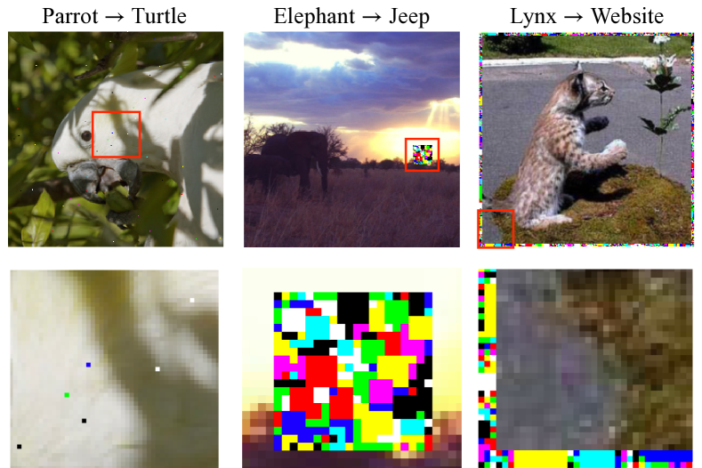
Figure 1: Adversarial examples for sparse threat models ($\l_{0}$-bounded, patches, frames) generated with our black-box Sparse-RS framework which does not require surrogate models and is more query efficient.

Conversely, sparse attacks pursue an opposite strategy: they perturb only a small portion of the original input but possibly with large modifications. Thus, the perturbations are indeed visible but do not alter the semantic content, and can even be applied in the physical world (Lee and Kolter 2019; Thys, Van Ranst, and Goedemé 2019; Li, Schmidt, and Kolter 2019). Sparse attacks include $l_{0}$-attacks (Narodytska and Kasiviswanathan 2017; Carlini and Wagner 2017; Papernot et al. 2016; Schott et al. 2019; Croce and Hein 2019), adversarial patches (Brown et al. 2017; Karmon, Zoran, and Goldberg 2018; Lee and Kolter 2019) and frames (Zajac et al. 2019), where the perturbations have some predetermined structure. Moreover, sparse attacks generalize to tasks outside computer vision, such as malware detection or natural language processing, where the nature of the domain imposes to modify only a limited number of input features (Grosse et al. 2016; Jin et al. 2019).

We focus on the black-box score-based scenario, where the attacker can only access the predicted scores of a classifier $f$, but does not know the network weights and in particularly cannot use gradients of $f$ wrt the input (as in the white-box setup). We do not consider more restrictive (e.g., decision-based attacks (Brendel, Rauber, and Bethge 2018; Brunner et al. 2019) where the adversary only knows the label assigned to each input) or more permissive (e.g., a surrogate model similar to the victim one is available (Cheng et al. 2019; Huang and Zhang 2020)) cases. For the $l_{0}$-threat model only a few black-box attacks exist (Narodytska and Kasiviswanathan 2017; Schott et al. 2019; Croce and Hein 2019; Zhao et al. 2019), which however do not focus on query efficiency or scale to datasets like ImageNet without suffering from prohibitive computational cost. For adversarial patches and frames, black-box methods are mostly limited to transfer attacks, that is a white-box attack is performed on a surrogate model, with the exception of (Yang et al. 2020) who use a predefined dictionary of patches.

Contributions. Random search is particularly suitable for zeroth-order optimization in presence of complicated combinatorial constraints, as those of sparse threat models. Then, we design specific sampling distributions for the random search algorithm to efficiently generate sparse black-box attacks. The resulting Sparse-RS is a simple and flexible framework which handles

• $l_{0}$-perturbations: Sparse-RS significantly outperforms the existing black-box attacks in terms of the query efficiency and success rate, and leads to a better success rate even when compared to the state-of-the-art white-box attacks on standard and robust models.

• Adversarial patches: Sparse-RS achieves better results than both TPA (Yang et al. 2020) and a black-box adaptations of projected gradient descent (PGD) attacks via gradient estimation.

• Adversarial frames: Sparse-RS outperforms the existing adversarial framing method (Zajac et al. 2019) with gradient estimation and achieves a very high success rate even with 2-pixel wide frames.

Due to space reasons the results for adversarial frames had to be moved to the appendix.

2 Black-box adversarial attacks

Let $f:\mathcal{S}\subseteq\mathbb{R}^{d}\rightarrow\mathbb{R}^{K}$ be a classifier which assigns input $x\in\mathcal{S}$ to class $y=\text{arg\,max}_{r=1,\ldots,K}f_{r}(x)$. The goal of an untargeted attack is to craft a perturbation $\delta\in\mathbb{R}^{d}$ s.t.

$$\mathop{\rm arg\,max}\limits_{r=1,\ldots,K}f_{r}(x+\delta)\neq y,\quad x+\delta\in\mathcal{S}\quad\text{and}\quad\delta\in\mathcal{T},$$

where $\mathcal{S}$ is the input domain and $\mathcal{T}$ are the constraints the adversarial perturbation has to fulfill (e.g. bounded $l_{p}$-norm), while a targeted attack aims at finding $\delta$ such that

$$\mathop{\rm arg\,max}\limits_{r=1,\ldots,K}f_{r}(x+\delta)=t,\quad x+\delta\in\mathcal{S}\quad\text{and}\quad\delta\in\mathcal{T},$$

with $t$ as target class. Generating such $\delta$ can be translated into an optimization problem as

$$\min\limits_{\delta\in\mathbb{R}^{d}}\;L(f(x+\delta),t)\quad\text{s.t.}\quad x+\delta\in\mathcal{S}\quad\text{and}\quad\delta\in\mathcal{T}$$ (1)

by choosing a label $t$ and loss function $L$ whose minimization leads to the desired classification. By threat model we mean the overall attack setting determined by the goal of the attacker (targeted vs untargeted attack), the level of knowledge (white- vs black-box), and the perturbation set $\mathcal{T}$.

Many algorithms have been proposed to solve Problem (1) in the black-box setting where one cannot use gradient-based methods. One of the first approaches is by (Fawzi and Frossard 2016) who propose to sample candidate adversarial occlusions via the Metropolis MCMC method, which can be seen as a way to generate adversarial patches whose content is not optimized. (Ilyas et al. 2018; Uesato et al. 2018) propose to approximate the gradient through finite difference methods, later improved to reduce their high computational cost in terms of queries of the victim models (Bhagoji et al. 2018; Tu et al. 2019; Ilyas, Engstrom, and Madry 2019). Alternatively, (Alzantot et al. 2019; Liu et al. 2019) use genetic algorithms in the context of image classification and malware detection respectively. A line of research has focused on rephrasing $l_{\infty}$-attacks as discrete optimization problems (Moon, An, and Song 2019; Al-Dujaili and O’Reilly 2020; Meunier, Atif, and Teytaud 2019), where specific techniques lead to significantly better query efficiency. (Guo et al. 2019) adopt a variant of random search to produce perturbations with a small $l_{2}$-norm.

Closest in spirit is the Square Attack of (Andriushchenko et al. 2020), which is state-of-the-art for $l_{\infty}$- and $l_{2}$-bounded black-box attacks. It uses random search to iteratively generate samples on the surface of the $l_{\infty}$- or $l_{2}$-ball. Together with a particular sampling distribution based on square-shaped updates and a specific initialization, this leads to a simple algorithm which outperforms more sophisticated attacks in success rate and query efficiency. In this paper we show that the random search idea is ideally suited for sparse attacks, where the non-convex, combinatorial constraints are not easily handled even by gradient-based white-box attacks.

3 Sparse-RS framework

Random search (RS) is a well known scheme for derivative free optimization (Rastrigin 1963). Given an objective function $L$ to minimize, a starting point $x^{(0)}$ and a sampling distribution $\mathcal{D}$, an iteration of RS at step $i$ is given by

$$\delta\sim\mathcal{D}(x^{(i)}),\quad x^{(i+1)}=\mathop{\rm arg\,min}\limits_{y\in\{x^{(i)},\,x^{(i)}+\delta\}}L(y).$$ (2)

At every step an update of the current iterate $x^{(i)}$ is sampled according to $\mathcal{D}$ and accepted only if it decreases the objective value, otherwise the procedure is repeated. Although not explicitly mentioned in Eq. (2), constraints on the iterates $x^{(i)}$ can be integrated by ensuring that $\delta$ is sampled so that $x^{(i)}+\delta$ is a feasible solution. Thus even complex, e.g. combinatorial, constraints can easily be integrated as RS just needs to be able to produce feasible points in contrast to gradient-based methods which depend on a continuous set to optimize over. While simple and flexible, RS is an effective tool in many tasks (Zabinsky 2010; Andriushchenko et al. 2020), with the key ingredient for its success being a task-specific sampling distribution $\mathcal{D}$ to guide the exploration of the space of possible solutions.

input : loss $L$, input $x_{\textrm{orig}}{}$, max query $N$, sparsity $k$, input space constraints $\mathcal{S}$

output : approximate minimizer of $L$

1 $M\leftarrow$ $k$ indices of elements to be perturbed

2 $\Delta\leftarrow$ values of the perturbation to be applied

3 $z\leftarrow x_{\textrm{orig}}{}$,  $z_{M}\leftarrow\Delta$   // set elements in $M$ to values in $\Delta$

4 $L^{*}\leftarrow L(z)$,  $i\leftarrow 0$   // initialize loss

5 while $i<N$ and success not achieved do

6       $M^{\prime}\leftarrow$ sampled modification of $M$

7       // new set of indices

8       $\Delta^{\prime}\leftarrow$ sampled modification of $\Delta$

9       // new perturbation

10       $z\leftarrow x_{\textrm{orig}}{}$,  $z_{M^{\prime}}\leftarrow\Delta^{\prime}$

11       // create new candidate in $\mathcal{S}$

12       if $L(z)<L^{*}$ then

13             $L^{*}\leftarrow L(z)$,   $M\leftarrow M^{\prime}$,   $\Delta\leftarrow\Delta^{\prime}$   // if loss improves, update sets

14      $i\leftarrow i+1$

15$z\leftarrow x_{\textrm{orig}}{}$,  $z_{M}\leftarrow\Delta$   // return best $\Delta$

return $z$

Algorithm 1 Sparse-RS

We summarize our general framework based on random search to generate sparse adversarial attacks, Sparse-RS, in Alg. 1, where the sparsity $k$ indicates the maximum number of features that can be perturbed. A sparse attack is characterized by two variables: the set of components to be perturbed $M$ and the values $\Delta$ to be inserted at $M$ to form the adversarial input. To optimize over both of them we first sample a random update of the locations $M$ of the current perturbation (step 6) and then a random update of its values $\Delta$ (step 7). In some threat models (e.g. adversarial frames) the set $M$ cannot be changed, so $M^{\prime}\equiv M$ at every step. How $\Delta^{\prime}$ is generated depends on the specific threat model, so we present the individual procedures in the next sections. We note that for all threat models, the runtime is dominated by the cost of a forward pass through the network, and all other operations are computationally inexpensive.

Common to all variants of Sparse-RS is that the whole budget for the perturbations is fully exploited both in terms of number of modified components and magnitude of the elementwise changes (constrained only by the limits of the input domain $\mathcal{S}$). This follows the intuition that larger perturbations should lead faster to an adversarial example. Moreover, the difference of the candidates $M^{\prime}$ and $\Delta^{\prime}$ with $M$ and $\Delta$ shrinks gradually with the iterations which mimics the reduction of the step size in gradient-based optimization: initial large steps allow to quickly decrease the objective loss, but smaller steps are necessary to refine a close-to-optimal solution at the end of the algorithm. Finally, we impose a limit $N$ on the maximum number of queries of the classifier, i.e. evaluations of the objective function.

As objective function $L$ to be minimized, we use in the case of untargeted attacks the margin loss $L_{\text{margin}}(f(\cdot),y)=f_{y}(\cdot)-\max_{r\neq y}f_{r}(\cdot)$, where $y$ is the correct class, so that $L<0$ is equivalent to misclassification, whereas for targeted attacks we use the cross-entropy loss $L_{\text{CE}}$ of the target class $t$, namely $L_{\text{CE}}(f(\cdot),t)=-f_{t}(\cdot)+\log\left(\sum_{r=1}^{K}e^{f_{r}(\cdot)}\right)$.

The code of the Sparse-RS framework is available at https://github.com/fra31/sparse-rs.

4 Sparse-RS for $l_{0}$-bounded attacks

The first threat model we consider are $l_{0}$-bounded adversarial examples where only up to $k$ pixels or $k$ features/color channels of an input $x_{\textrm{orig}}{}\in[0,1]^{h\times w\times c}$ (width $w$, height $h$, color $c$) can be modified, but there are no constraints on the magnitude of the perturbations except for those of the input domain. Note that constraining the number of perturbed pixels or features leads to two different threat models which are not directly comparable. Due to the combinatorial nature of the $l_{0}$-threat model, this turns out to be quite difficult for continuous optimization techniques which are more prone to get stuck in suboptimal maxima.

$l_{0}$-RS algorithm. We first consider the threat model where up to $k$ pixels can be modified. Let $U$ be the set of the $h\cdot w$ pixels. In this case the set $M\subset U$ from Alg. 1 is initialized sampling uniformly $k$ elements of $U$, while $\Delta\sim\mathcal{U}(\{0,1\}^{k\times c})$, that is random values in $\{0,1\}$ (every perturbed pixel gets one of the corners of the color cube $[0,1]^{c}$). Then, at the $i$-th iteration, we randomly select $A\subset M$ and $B\subset U\setminus M$, with $|A|=|B|=\alpha^{(i)}\cdot k$, and create $M^{\prime}=(M\setminus A)\cup B$. $\Delta^{\prime}$ is formed by sampling random values from $\{0,1\}^{c}$ for the elements in $B$, i.e. those which were not perturbed at the previous iteration. The quantity $\alpha^{(i)}$ controls how much $M^{\prime}$ differs from $M$ and decays following a predetermined piecewise constant schedule rescaled according to the maximum number of queries $N$. The schedule is completely determined by the single value $\alpha_{\text{init}}$, used to calculate $\alpha^{(i)}$ for every iteration $i$, which is also the only free hyperparameter of our scheme. We provide details about the algorithm, schedule, and values of $\alpha_{\text{init}}$ in App. A and B, and ablation studies for them in App. G. For the feature based threat model each color channel is treated as a pixel and one applies the scheme above to the “gray-scale” image ($c=1$) with three times as many “pixels”.

4.1 Comparison of query efficiency of $l_{0}$-RS

We compare pixel-based $l_{0}$-RS to other black-box untargeted attacks in terms of success rate versus query efficiency. The results of targeted attacks are in App. A. Here we focus on attacking normally trained VGG-16-BN and ResNet-50 models on ImageNet, which contains RGB images resized to shape $224\times 224$, that is 50,176 pixels, belonging to 1,000 classes. We consider perturbations of size $k\in\{50,150\}$ pixels to assess the effectiveness of the untargeted attacks at different thresholds with a limit of 10,000 queries. We evaluate the success rate on the initially correctly classified images out of 500 images from the validation set.

Competitors. Many existing black-box pixel-based $l_{0}$-attacks (Narodytska and Kasiviswanathan 2017; Schott et al. 2019; Croce and Hein 2019) do not aim at query efficiency and rather try to minimize the size of the perturbations. Among them, only CornerSearch (Croce and Hein 2019) and ADMM attack (Zhao et al. 2019) scale to ImageNet. However, CornerSearch requires $8\times\#pixels$ queries only for the initial phase, exceeding the query limit we fix by more than $40$ times. The ADMM attack tries to achieve a successful perturbation and then reduces its $l_{0}$-norm. Moreover, we introduce black-box versions of PGD_$0$ (Croce and Hein 2019) with the gradient estimated by finite difference approximation as done in prior work, e.g., see (Ilyas et al. 2018). As a strong baseline, we introduce JSMA-CE which is a version of the JSMA algorithm (Papernot et al. 2016) that we adapt to the black-box setting: (1) for query efficiency, we estimate the gradient of the cross-entropy loss instead of gradients of each class logit, (2) on each iteration, we modify the pixels with the highest gradient contribution. More details about the attacks can be found in App. A.

VGG ResNet

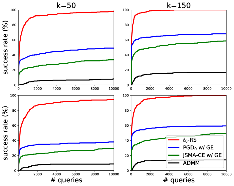
Figure 2: Progression of the success rate vs number of queries for black-box pixel-based $l_{0}$-attacks on ImageNet in the untargeted setting. At all sparsity levels $l_{0}$-RS (red) outperforms PGD_$0$ (blue) and JSMA-CE (green) with gradient estimation and ADMM attack (black).

Figure 3: Untargeted $l_{0}$-adversarial examples generated by our pixel-based $l_{0}$-RS algorithm for $k=50$ pixels.

Results. We show in Fig. 2 the success rate vs the number of queries for all black-box attacks. In all cases, $l_{0}$-RS outperforms its competitors in terms of the final success rate by a large margin—the second best method (PGD_$0$ w/ GE) is at least 30% worse. Moreover, $l_{0}$-RS is query efficient as it achieves results close to the final ones already with a low number of queries. For example, on VGG with $k=150$, $l_{0}$-RS achieves $100\%$ of success rate using on average only 171 queries, with a median of 25. Unlike other methods, $l_{0}$-RS can achieve almost 100% success rate by perturbing 50 pixels which is only 0.1% of the total number of pixels. We visualize the adversarial examples of $l_{0}$-RS in Fig. 3.

4.2 Using $l_{0}$-RS for accurate robustness evaluation

In this section, our focus is the accurate evaluation of robustness in the $l_{0}$-threat model. For this, we evaluate existing white-box methods and black-box methods together. Instead of the success rate taken only over correctly classified examples, here we rather consider robust error (similarly to (Madry et al. 2018)), which is defined as the classification error on the adversarial examples crafted by an attacker.

attack	type	VGG	ResNet
$l_{0}$-bound in pixel space $k=50$
JSMA-CE	white-box	42.6%	39.6%
PGD$0$	white-box	87.0%	81.2%
ADMM	black-box	30.3%	29.0%
JSMA-CE with GE	black-box	49.6%	44.8%
PGD$0$ with GE	black-box	61.4%	51.8%
CornerSearch∗	black-box	82.0%	72.0%
$l_{0}$-RS	black-box	98.2%	95.8%
$l_{0}$-bound in feature space $k=50$
SAPF∗	white-box	21.0%	18.0%
ProxLogBarrier	white-box	33.0%	28.4%
EAD	white-box	39.8%	35.6%
SparseFool	white-box	43.6%	42.0%
VFGA	white-box	58.8%	55.2%
FMN	white-box	83.8%	77.6%
PDPGD	white-box	89.6%	87.2%
ADMM	black-box	32.6%	29.0%
CornerSearch∗	black-box	76.0%	62.0%
$l_{0}$-RS	black-box	92.8%	88.8%

Table 1: ImageNet: Robust test error of $l_{0}$-attacks. The entries with ^∗ are evaluated on 100 points instead of 500 because of their high computational cost. All black-box attacks use 10k queries except CornerSearch which uses 600k. $l_{0}$-RS outperforms all black- and white-box attacks.

White-box attacks on ImageNet. We test the robustness of the ImageNet models introduced in the previous section to $l_{0}$-bounded perturbations. As competitors we consider multiple white-box attacks which minimize the $l_{0}$-norm in feature space: SAPF (Fan et al. 2020), ProxLogBarrier (Pooladian et al. 2020), EAD (Chen et al. 2018), SparseFool (Modas, Moosavi-Dezfooli, and Frossard 2019), VFGA (Césaire et al. 2020), FMN (Pintor et al. 2021) and PDPGD (Matyasko and Chau 2021). For the $l_{0}$-threat model in pixel space we use two white-box baselines: PGD₀ (Croce and Hein 2019), and JSMA-CE (Papernot et al. 2016) (where we use the gradient of the cross-entropy loss to generate the saliency map). Moreover, we show the results of the black-box attacks from the previous section (all with a query limit of 10,000), and additionally use the black-box CornerSearch for which we use a query limit of 600k and which is thus only partially comparable. Details of the attacks are available in App. A. Table 1 shows the robust error given by all competitors: $l_{0}$-RS achieves the best results for pixel and feature based $l_{0}$-threat model on both VGG and ResNet, outperforming black- and white-box attacks. We note that while the PGD attack has been observed to give accurate robustness estimates for $l_{\infty}$- and $l_{2}$-norms (Madry et al. 2018), this is not the case for the $l_{0}$ constraint set. This is due to the discrete structure of the $l_{0}$-ball which is not amenable for continuous optimization.

attack	type	$l_{2}$-AT ResNet	$l_{1}$-AT ResNet
$l_{0}$-bound in pixel space $k=24$
PGD0	white-box	68.7%	72.7%
CornerSearch	black-box	59.3%	64.9%
$l_{0}$-RS	black-box	85.7%	81.0%
$l_{0}$-bound in feature space $k=24$
VFGA	white-box	40.5%	27.5%
FMN	white-box	52.9%	28.2%
PDPGD	white-box	46.4%	26.9%
CornerSearch	black-box	43.2%	29.4%
$l_{0}$-RS	black-box	63.4%	38.3%

Table 2: CIFAR10: Robust test error of untargeted $l_{0}$-attacks in pixel and feature space on a $l_{2}$- resp. $l_{1}$-AT model.

Comparison on CIFAR-10. In Table 2 we compare the strongest white- and black-box attacks on $l_{1}$- resp. $l_{2}$-adversarially trained PreAct ResNet-18 on CIFAR-10 from (Croce and Hein 2021) and (Rebuffi et al. 2021) (details in App. A.5). We keep the same computational budget used on ImageNet. As before, we consider perturbations with $l_{0}$-norm $k=24$ in pixel or feature space: in both cases $l_{0}$-RS achieves the highest robust test error outperforming even all white-box attacks. Note that, as expected, the model robust wrt $l_{1}$ is less vulnerable to $l_{0}$-attacks especially in the feature space, whose $l_{1}$-norm is close to that used during training.

Robust generative models on MNIST. (Schott et al. 2019) propose two robust generative models on MNIST, ABS and Binary ABS, which showed high robustness against multiple types of $l_{p}$-bounded adversarial examples. These classifiers rely on optimization-based inference using a variational auto-encoder (VAE) with 50 steps of gradient descent for each prediction (times 1,000 repetitions). It is too expensive to get gradients with respect to the input through the optimization process, thus (Schott et al. 2019) evaluate only black-box attacks, and test $l_{0}$-robustness with sparsity $k=12$ using their proposed Pointwise Attack with 10 restarts. We evaluate on both models CornerSearch with a budget of 50,000 queries and $l_{0}$-RS with an equivalent budget of 10,000 queries and $5$ random restarts. Table 3 summarizes the robust test error (on 100 points) achieved by the attacks (the results of Pointwise Attack are taken from (Schott et al. 2019)). For both classifiers, $l_{0}$-RS yields the strongest evaluation of robustness suggesting that the ABS models are less robust than previously believed. This illustrates that despite we have full access to the attacked VAE model, a strong black-box $l_{0}$-attack can still be useful for an accurate robustness evaluation.

attack	type	$k=12$ (pixels)
		ABS	Binary ABS
Pointwise Attack	black-box	31%	23%
CornerSearch	black-box	29%	28%
$l_{0}$-RS	black-box	55%	51%

Table 3: Robust test error on robust models (Schott et al. 2019) on MNIST by different attacks on 100 test points.

$l_{0}$-RS on malware detection. We apply our method on a malware detection task and show its effectiveness in App. B.

4.3 Theoretical analysis of $l_{0}$-RS

Given the empirical success of $l_{0}$-RS, here we analyze it theoretically for a binary classifier. While the analysis does not directly transfer to neural networks, most modern neural network architectures result in piecewise linear classifiers (Arora et al. 2018), so that the result approximately holds in a sufficiently small neighborhood of the target point $x$.

As in the malware detection task in App. B, we assume that the input $x$ has binary features, $x\in\{0,1\}^{d}$, and we denote the label by $y\in\{-1,1\}$ and the gradient of the linear model by $w_{x}\in\mathbb{R}^{d}$. Then the Problem (1) of finding the optimal $l_{0}$ adversarial example is equivalent to:

$$\mathop{\rm arg\,min}\limits_{\begin{subarray}{c}\left\|\delta\right\|_{0}\leq k\\ x_{i}+\delta_{i}\in\{0,1\}\end{subarray}}y\left\langle w_{x},x+\delta\right\rangle =\mathop{\rm arg\,min}\limits_{\begin{subarray}{c}\left\|\delta\right\|_{0}\leq k\\ \delta_{i}\in\{0,1-2x_{i}\}\end{subarray}}\left\langle yw_{x},\delta\right\rangle$$

$$=\mathop{\rm arg\,min}\limits_{\begin{subarray}{c}\left\|\delta\right\|_{0}\leq k\\ \delta_{i}\in\{0,1\}\end{subarray}}\hskip 3.0pt\langle\underbrace{yw_{x}\odot(1-2x)}_{\hat{w}_{x}},\delta\rangle,$$

where $\odot$ denotes the elementwise product. In the white-box case, i.e. when $w_{x}$ is known, the solution is to simply set $\delta_{i}=1$ for the $k$ smallest weights of $\hat{w}_{x}$. The black-box case, where $w_{x}$ is unknown and we are only allowed to query the model predictions $\left\langle\hat{w}_{x},z\right\rangle$ for any $z\in\mathbb{R}^{d}$, is more complicated since the naive weight estimation algorithm requires $O(d)$ queries to first estimate $\hat{w}_{x}$ and then to perform the attack by selecting the $k$ minimal weights. This naive approach is prohibitively expensive for high-dimensional datasets (e.g., $d=150{,}528$ on ImageNet assuming $224\times 224\times 3$ images). However, the problem of generating adversarial examples does not have to be always solved exactly, and often it is enough to find an approximate solution. Therefore we can be satisfied with only identifying $k$ among the $m$ smallest weights. Indeed, the focus is not on exactly identifying the solution but rather on having an algorithm that in expectation requires a sublinear number of queries. With this goal, we show that $l_{0}$-RS satisfies this requirement for large enough $m$.

Proposition 4.1

The expected number $t_{k}$ of queries needed for $l_{0}$-RS with $\alpha^{(i)}=\nicefrac{{1}}{{k}}$ to find a set of $k$ weights out of the smallest $m$ weights of a linear model is:

$$\mathbb{E}\left[t_{k}\right]=(d-k)k\sum_{i=0}^{k-1}\frac{1}{(k-i)(m-i)}<(d-k)k\frac{\ln(k)+2}{m-k}.$$

		attack	VGG			ResNet
			success rate	mean queries	med. queries	success rate	mean queries	med. queries
untarget. $20\times 20$	black-box	LOAP w/ GE	55.1% $\pm$ 0.6	5879 $\pm$ 51	7230 $\pm$ 377	40.6% $\pm$ 0.1	6870 $\pm$ 10	10000 $\pm$ 0
		TPA	46.1% $\pm$ 1.1	6085* $\pm$ 83	8080* $\pm$ 1246	49.0% $\pm$ 1.2	5722* $\pm$ 64	5280* $\pm$ 593
		Sparse-RS + SH	82.6%	2479	514	75.3%	3290	549
		Sparse-RS + SA	85.6% $\pm$ 1.1	2367 $\pm$ 83	533 $\pm$ 40	78.5% $\pm$ 1.0	2877 $\pm$ 64	458 $\pm$ 43
		Patch-RS	87.8% $\pm$ 0.7	2160 $\pm$ 44	429 $\pm$ 22	79.5% $\pm$ 1.4	2808 $\pm$ 89	438 $\pm$ 68
2-9		White-box LOAP	98.3%	-	-	82.2%	-	-
targeted $40\times 40$	black-box	LOAP w/ GE	23.9% $\pm$ 0.9	44134 $\pm$ 71	50000 $\pm$ 0	18.4% $\pm$ 0.9	45370 $\pm$ 88	50000 $\pm$ 0
		TPA	5.1% $\pm$ 1.2	29934* $\pm$ 462	34000* $\pm$ 0	6.0% $\pm$ 0.5	31690* $\pm$ 494	34667* $\pm$ 577
		Sparse-RS + SH	63.6%	25634	19026	48.6%	31250	50000
		Sparse-RS + SA	70.9% $\pm$ 1.2	23749 $\pm$ 346	15569 $\pm$ 568	53.7% $\pm$ 0.9	32290 $\pm$ 239	40122 $\pm$ 2038
		Patch-RS	72.7% $\pm$ 0.9	22912 $\pm$ 207	14407 $\pm$ 866	55.6% $\pm$ 1.5	30290 $\pm$ 317	34775 $\pm$ 2660
2-9		White-box LOAP	99.4%	-	-	94.8%	-	-

Table 4: Success rate and query statistics of image-specific patches. Black-box attacks are given 10k/50k queries for untargeted/targeted case. SH is a deterministic method. The query statistics are computed on all images with 5 random seeds. ^∗ TPA uses an early stopping mechanism to save queries, thus might not use all queries. Patch-RS outperforms all other methods in success rate and query efficiency.

Untargeted patches			Targeted patches
Parrot $\rightarrow$ Torch	Castle $\rightarrow$ Traffic light	Speedboat $\rightarrow$ Amphibian	Bee eater $\rightarrow$ Tiger cat	Newfoundland $\rightarrow$ Bucket	Geyser $\rightarrow$ Racer

Figure 4: Image-specific untargeted ($20\times 20$ pixels) and targeted ($40\times 40$) patches generated by our Patch-RS algorithm.

The proof is deferred to App. F and resembles that of the coupon collector problem. For non-linear models, $l_{0}$-RS uses $\alpha^{(i)}>\nicefrac{{1}}{{k}}$ for better exploration initially, but then progressively reduces it. The main conclusion from Proposition 4.1 is that $\mathbb{E}\left[t_{k}\right]$ becomes sublinear for large enough gap $m-k$, as we illustrate in Fig. 11 in App. F.

5 Sparse-RS for adversarial patches

Another type of sparse attacks which recently received attention are adversarial patches introduced by (Brown et al. 2017). There the perturbed pixels are localized, often square-shaped, and limited to a small portion of the image but can be changed in an arbitrary way. While some works (Brown et al. 2017; Karmon, Zoran, and Goldberg 2018) aim at universal patches, which fool the classifier regardless of the image and the position where they are applied, which we consider in Sec. 6, we focus first on image-specific patches as in (Yang et al. 2020; Rao, Stutz, and Schiele 2020) where one optimizes both the content and the location of the patch for each image independently.

General algorithm for patches. Note that both location (step 6 in Alg. 1) and content (step 7 in Alg. 1) have to be optimized in Sparse-RS, and on each iteration we check only one of these updates. We test the effect of different frequencies of location/patch updates in an ablation study in App. G.2. Since the location of the patch is a discrete variable, random search is particularly well suited for its optimization. For the location updates in step 6 in Alg. 1, we randomly sample a new location in a 2D $l_{\infty}$-ball around the current patch position (using clipping so that the patch is fully contained in the image). The radius of this $l_{\infty}$-ball shrinks with increasing iterations in order to perform progressively more local optimization (see App. C for details).

For the update of the patch itself in step 7 in Alg. 1, the only constraints are given by the input domain $[0,1]^{d}$. Thus in principle any black-box method for an $l_{\infty}$-threat model can be plugged in there. We use Square Attack (SA) (Andriushchenko et al. 2020) and SignHunter (SH) (Al-Dujaili and O’Reilly 2020) as they represent the state-of-the-art in terms of success rate and query efficiency. We integrate both in our framework and refer to them as Sparse-RS + SH and Sparse-RS + SA. Next we propose a novel random search based attack motivated by SA which together with our location update yields our novel Patch-RS attack.

Patch-RS. While SA and SH are state-of-the-art for $l_{\infty}$-attacks, they have been optimized for rather small perturbations whereas for patches all pixels can be manipulated arbitrarily in $[0,1]$. Here, we design an initialization scheme and a sampling distribution specific for adversarial patches. As initialization (step 2 of Alg. 1), Patch-RS uses randomly placed squares with colors in $\{0,1\}^{3}$, then it samples updates of the patch (step 7) with shape of squares, of size decreasing according to a piecewise constant schedule, until a refinement phase in the last iterations, when it performs single-channel updates (exact schedule in App. C). This is in contrast to SA where random vertical stripes are used as initialization and always updates for all three channels of a pixel are sampled. The ablation study in App. G.2 shows how both modifications contribute to the improved performance of Patch-RS.

Experiments. In addition to Sparse-RS + SH, Sparse-RS + SA, and Patch-RS, we consider two existing methods. i) TPA (Yang et al. 2020) which is a black-box attack aiming to produce image-specific adv. patches based on reinforcement learning. While (Yang et al. 2020) allows multiple patches for an image, we use TPA in the standard setting of a single patch. ii) Location-Optimized Adversarial Patches (LOAP) (Rao, Stutz, and Schiele 2020), a white-box attack that uses PGD for the patch updates, which we combine with gradient estimation in order to use it in the black-box scenario (see App. C for details). In Table 4 we report success rate, mean and median number of queries used for untargeted attacks with patch size $20\times 20$ and query limit of 10,000 and for targeted attacks (random target class for each image) with patch size $40\times 40$ and maximally 50,000 queries. We attack 500 images of ImageNet with VGG and ResNet as target models. The query statistics are computed on all 500 images, i.e. without restricting to only successful adversarial examples, as this makes the query efficiency comparable for different success rates. Our Sparse-RS + SH, Sparse-RS + SA and Patch-RS outperform existing methods by a large margin, showing the effectiveness of our scheme to optimize both location and patch. Among them, our specifically designed Patch-RS achieves the best results in all metrics. We visualize its resulting adversarial examples in Fig. 4.

6 Universal adversarial patches

A challenging threat model is that of a black-box, targeted universal adversarial patch attack where the classifier should be fooled into a chosen target class when the patch is applied inside any image of some other class. Previous works rely on transfer attacks: in (Brown et al. 2017) the universal patch is created using a white-box attack on surrogate models, while the white-box attack of (Karmon, Zoran, and Goldberg 2018) directly optimizes the patch for the target model on a set of training images and then only tests generalization to unseen images. Our goal is a targeted black-box attack which crafts universal patches that generalize to unseen images when applied at random locations (see examples in Fig. 5). To our knowledge, this is the first method for this threat model which does not rely on a surrogate model.
We employ Alg. 1 where for the creation of the patches in step 7 we use either SH, SA or our novel sampling distribution introduced in Patch-RS in Sec. 5. The loss in Alg. 1 is computed on a small batch of 30 training images and the initial locations $M$ of the patch in each of the training images are sampled randomly. In order not to overfit on the training batch, we resample training images and locations of the patches (step 6 in Alg. 1) every $10k$ queries (total query budget $100k$). As stochastic gradient descent this is a form of stochastic optimization of the population loss (expectation over images and locations) via random search.

Experiments. We apply the above scheme to Sparse-RS + SH/SA and Patch-RS to create universal patches of size $50\times 50$ for 10 random target classes on VGG (we repeat it for 3 seeds for RS-based methods). We compare to (1) the transfer-based attacks obtained via PGD (Madry et al. 2018) and MI-FGSM (Dong et al. 2018) using ResNet as surrogate model, and to (2) ZO-AdaMM (Chen et al. 2019) based on gradient estimation. The results in Table 5 show that our Sparse-RS + SH/SA and Patch-RS outperform other methods by large margin. We provide extra details and results for frames in App. E.

attack	VGG
Transfer PGD	3.3%
Transfer MI-FGSM	1.3%
PGD w/ GE	35.1%
ZO-AdaMM	45.8%
Sparse-RS + SH	63.9%
Sparse-RS + SA	72.9% $\pm$ 3.6
Patch-RS	70.8% $\pm$ 1.3

Table 5: Success rate of targeted universal $50\times 50$ patches.

Targeted universal patches
Butterfly $\rightarrow$ Rottweiler	Persian cat $\rightarrow$ Slug	Starfish $\rightarrow$ Polecat
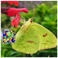
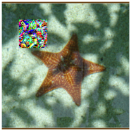
Echidna $\rightarrow$ Rottweiler	Geyser $\rightarrow$ Slug	Electric guitar $\rightarrow$ Polecat

Figure 5: We visualize two images in each column with the same targeted universal patch generated by Patch-RS that changes the predictions to the desired target class.

7 Conclusion

We propose a versatile framework, Sparse-RS, which achieves state-of-the-art success rate and query efficiency in multiple sparse threat models: $l_{0}$-perturbations, adversarial patches and adversarial frames (see App. D). Moreover, it is effective in the challenging task of crafting universal adversarial patches without relying on surrogate models, unlike the existing methods. We think that strong black-box adversarial attacks are a very important component to assess the robustness against such localized and structured attacks, which go beyond the standard $l_{p}$-threat models.

Appendix

Organization of the appendix

The appendix contains several additional results that we omitted from the main part of the paper due to the space constraints, as well as additional implementation details for each method. The organization of the appendix is as follows:

• Sec. A: additional results and implementation details of $l_{0}$-bounded attacks where we also present results of targeted attacks on ImageNet.

• Sec. B: $l_{0}$-bounded attacks on malware detection.

• Sec. C: implementation details for generating image- and location-specific adversarial patches.

• Sec. D: image-specific adversarial frames with Sparse-RS.

• Sec. E: results of universal attacks, i.e. image- and location-independent attacks, which include targeted universal patches and targeted universal frames.

• Sec. F: theoretical analysis of the $l_{0}$-RS algorithm.

• Sec. G: ablation studies for $l_{0}$-RS and Patch-RS.

Appendix A $l_{0}$-bounded attacks: image classification

In this section, we first describe the results of targeted attacks, then we show additional statistics for untargeted attacks, and describe the hyperparameters used for $l_{0}$-RS and competing methods.

A.1 Targeted attacks

Here we test $l_{0}$-bounded attacks in the targeted scenario using the sparsity level $k=150$ (maximum number of perturbed pixels or features) on ImageNet. For black-box attacks including $l_{0}$-RS, we set the query budget to $100,000$, and show the success rate on VGG and ResNet in Table 6 computed on $500$ points. We also give additional budget to white-box attacks compared to the untargeted case (see details in App. A.4). The target class for each point is randomly sampled from the set of labels which excludes the true label. We report the success rate in Table 6 instead of robust error since we are considering targeted attacks where the overall goal is to cause a misclassification towards a particular class instead of an arbitrary misclassification. We can see that targeted attacks are more challenging than untargeted attacks for many methods, particularly for methods like CornerSearch that were designed primarily for untargeted attacks. When considering the pixel space, $l_{0}$-RS outperforms both black- and white-box attacks, while in the feature space it is second only to PDPGD although achieving similar results on the VGG model.

Additionally, we report the query efficiency curves in Fig. 6 for $l_{0}$-RS, PGD₀ and JSMA-CE with gradient estimation. We omit the ADMM attack since it has shown the lowest success rate in the untargeted setting. We can see that $l_{0}$-RS achieves a high success rate (90%/80% for VGG/ResNet) even after 20,000 queries. At the same time, the targeted setting is very challenging for other methods that have nearly 0% success rate even after 100,000 queries. Finally, we visualize targeted $l_{0}$ adversarial examples generated by pixel-based $l_{0}$-RS in Fig. 7.

attack	type	VGG	ResNet
$l_{0}$-bound in pixel space $k=150$
JSMA-CE	white-box	0.4%	1.4%
PGD$0$	white-box	62.8%	67.8%
JSMA-CE w/ GE	black-box	0.0%	0.0%
PGD$0$ w/ GE	black-box	0.4%	1.4%
CornerSearch∗	black-box	3.0%	2.0%
$l_{0}$-RS	black-box	98.2%	95.6%
$l_{0}$-bound in feature space $k=150$
FMN	white-box	73.0%	79.8%
PDPGD	white-box	92.8%	94.2%
$l_{0}$-RS	black-box	90.8%	80.0%

Table 6: Success rate of targeted $l_{0}$-attacks on ImageNet. The entry with ^∗ is evaluated on 100 points instead of 500 because of their high computational cost. All black-box attacks use 100k queries except CornerSearch which uses 450k. $l_{0}$-RS outperforms all black- and white-box attacks in the pixel space scenario, and is competitive with white-box attacks in the feature space one.

VGG

ResNet

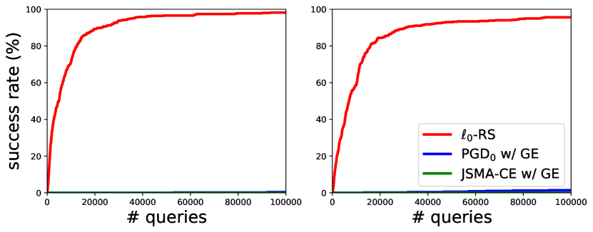
Figure 6: Success rate over queries for targeted black-box attacks in the pixel-based $l_{0}$-threat model with $k=150$.

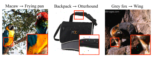
Figure 7: Targeted $l_{0}$ adversarial examples generated by our pixel-based $l_{0}$-RS algorithm for $k=150$ pixels.

A.2 Additional statistics for targeted and untargeted attacks

In Table 7, we report the details of success rate and query efficiency of the black-box attacks on ImageNet for sparsity levels $k\in\{50,150\}$ in the pixel space and 10,000/100,000 query limit for untargeted/targeted attacks respectively.

	pixels	attack	VGG			ResNet
	modified		succ. rate	mean queries	med. queries	succ. rate	mean queries	med. queries
untargeted	$k=50$	ADMM	8.3%	9402	10000	8.8%	9232	10000
		JSMA-CE w/ GE	33.5%	7157	10000	29.0%	7509	10000
		PGD0 w/ GE	49.1%	5563	10000	38.0%	6458	10000
		$l_{0}$-RS	97.6%	737	88	94.6%	1176	150
	$k=150$	ADMM	16.9%	8480	10000	14.2%	8699	10000
		JSMA-CE w/ GE	58.8%	4692	2460	49.4%	5617	10000
		PGD0 w/ GE	68.1%	3447	42	59.4%	4263	240
		$l_{0}$-RS	100%	171	25	100%	359	49
targeted	$k=150$	JSMA-CE w/ GE	0.0%	100000	100000	0.0%	100000	100000
		PGD0 w/ GE	0.4%	99890	100000	1.4%	99357	100000
		$l_{0}$-RS	98.2%	9895	4914	95.6%	14470	6960

Table 7: We report the success rate and statistics about query consumption of black-box $l_{0}$-bounded attacks in the pixel space on ImageNet. We consider sparsity levels $k\in\{50,150\}$ and compute the average and median number of queries needed to generate adversarial examples on all correctly classified points.

A.3 $l_{0}$-RS algorithm

As mentioned in Sec. 4, at iteration $i$ the new set $M^{\prime}$ is formed modifying $\alpha^{(i)}\cdot k$ (rounded to the closest positive integer) elements of $M$ containing the currently modified dimensions (see step 6 in Alg. 1). Inspired by the step-size reduction in gradient-based optimization methods, we progressively reduce $\alpha^{(i)}$. Assuming $N=10,000$, the schedule of $\alpha^{(i)}$ is piecewise constant where the constant segments start at iterations $j\in\{0,50,200,500,1000,2000,4000,6000,8000\}$ with values $\nicefrac{{\alpha_{\text{init}}}}{{\beta_{j}}}$, $\beta_{j}\in\{2,4,5,6,8,10,12,15,20\}$. For a different maximum number of queries $N$, the schedule is linearly rescaled accordingly. In practice, we use $\alpha_{\text{init}}=0.3$ and $\alpha_{\text{init}}=0.1$ for the untargeted and targeted scenario respectively on ImageNet (for both pixel and feature space), $\alpha_{\text{init}}=0.3$ and $\alpha_{\text{init}}=0.1$ when considering the pixel and feature space respectively on CIFAR-10.

A.4 Competitors

SparseFool. We use SparseFool (Modas, Moosavi-Dezfooli, and Frossard 2019) in the original implementation and optimize the hyperparameter which controls the sparsity of the solutions (called $\lambda$, setting finally $\lambda=1$) to achieve the best results. we use 60 and 100 steps for ImageNet and CIFAR-10 (default value is 20), after checking that higher values do not lead to improved performance but significantly increase the computational cost. Note that SparseFool has been introduced for the $l_{1}$-threat model but can generate sparse perturbations which are comparable to $l_{0}$-attacks.

PGD_$0$. For PGD_$0$ (Croce and Hein 2019) we use 2,000 iterations (5,000 for targeted attacks) and step size $0.05\cdot d$ ($0.025\cdot d$ for targeted attacks) for ImageNet ($0.5\cdot d$ for CIFAR-10) where $d=224\times 224\times 3$ (resp. $d=32\times 32\times 3$) is the input dimension. PGD_$0$ with gradient estimation uses the same gradient step of PGD_$0$ but with step size $5\cdot d$ ($1\cdot d$ for targeted attacks). To estimate the gradient we use finite differences, similarly to (Ilyas et al. 2018), as shown in Alg. 2, with the current iterate as input $x$, $\eta=0.01/\sqrt{d}$ (in line with what suggested in (Ilyas, Engstrom, and Madry 2019) for this algorithm), $m=1$ and a zero vector as $p$. In case of targeted attacks we instead use $m=50$ (the budget of queries is also 10 times larger) and the current estimated gradient as $p$. We optimized the aforementioned parameters to achieve the best results and tested that sampling more points to better approximate the gradient at each iteration leads to similar success rate with worse query consumption.

input : loss function $L$, input point $x$, number of iterations $m$, step size $\eta$, prior estimation $p$

output : estimated gradient $g$

1 $g\leftarrow p$

2 for $i=1,\ldots,m$ do

3       $s\leftarrow\mathcal{N}(0,I)$

4       $l_{1}\leftarrow L(x+\eta\cdot s)$

5       $l_{2}\leftarrow L(x-\eta\cdot s)$

6       $g\leftarrow g+(l_{1}-l_{2})/(2\eta)\cdot s$

Algorithm 2 GradEst: Gradient estimation via finite differences

CornerSearch. For CornerSearch on ImageNet, we used the following hyperparameters: n_max $=500$, n_iter $=200$, n_classes $=1,000$ (i.e. all classes, which is the default option) for untargeted attacks and n_max $=1,500$, n_iter $=50,000$ for targeted attacks. We note that CornerSearch has a limited scalability to ImageNet as it requires $8\cdot 224\cdot 224=401,408$ queries only for the initial phase of the attack to obtain the orderings of pixels, and then for the second phase n_iter $\cdot$ n_classes $=200,000$ queries for untargeted attacks and n_iter $=50,000$ queries for targeted attacks. On CIFAR-10 we set n_max $=450$, n_iter $=1000$, n_classes $=10$, which amounts to more than $17,000$ queries of budget. Thus, CornerSearch requires significantly more queries compared to $l_{0}$-RS while achieving a lower success rate. Finally, we note that CornerSearch was designed to minimize the number of modified pixels, while we use it here for $l_{0}$-bounded attacks.

SAPF. For SAPF (Fan et al. 2020), we use the hyperparameters suggested in their paper and we use the second-largest logit as the target class for untargeted attacks. With these settings, the algorithm is still very expensive computationally, so we could evaluate it only on 100 points. Note that (Fan et al. 2020) report that SAPF achieves the average $l_{0}$-norm of at least 30,000 which is orders of magnitudes more than what we consider here. But we evaluate it for completeness as their goal is to obtain a sparse adversarial attack measured in terms of $l_{0}$.

ADMM. For ADMM (Zhao et al. 2019) we perform a grid search over the parameters to optimize the success rate and set ro=10, gama=4, binary_search_steps=500 and Query_iterations=20 (other parameters are used with the default values). Note that (Zhao et al. 2019) report results for the $l_{0}$-norm only on MNIST. We apply it to both pixel and feature space scenarios by minimizing the corresponding metric.

JSMA-CE. As mentioned in Sec. 4.1 we adapt the method introduce in (Papernot et al. 2016) to scale it to attack models on ImageNet. We build the saliency map as the gradient of the cross-entropy loss instead of using the gradient of the logits because ImageNet has 1000 classes and it would be very expensive to get gradients of each logit separately (particularly in the black-box settings where one has to first estimate them). Moreover, at each iteration we perturb the pixel which has the gradient with the largest $l_{1}$-norm, setting each channel to either 0 or 1 according to the sign of the gradient at it. We perform these iterations until the total sparsity budget is reached. For the black-box version, we modify the algorithm as follows: the gradient is estimated via finite difference approximation as in Alg. 2, the original image $x_{\textrm{orig}}{}$ as input throughout the whole procedure (this means that the prior $p$ is always the current estimation of the gradient). We found that this gives stronger results compared to an estimation of the gradient at a new iterate. We use the gradient estimation step size $\eta=0.01$. Then every 10 queries we perturb the $k$ pixels with the largest gradient as described above for the white-box attack and check whether this new image is misclassified (we do not count this extra query for the budget of 10k). This is in line with the version of the attack we use for the malware detection task described in detail in Sec. B.

EAD. We use EAD (Chen et al. 2018) from Foolbox (Rauber, Brendel, and Bethge 2017) with $l_{1}$ decision rule, regularization parameter $\beta=0.1$ optimized to achieve highest success rate in the $l_{0}$-threat model and 1000 iterations (other parameters as default). Note that EAD is a strong white-box attack for $l_{1}$ and we include it as additional baseline since it can generate sparse attacks.

VFGA. We use VFGA (Césaire et al. 2020) as implemented in Adversarial Library (Rony and Ben Ayed 2020) with the default parameters.

FMN. For the Fast Minimum-Norm attack (Pintor et al. 2021) we use the implementation of Adversarial Library (Rony and Ben Ayed 2020) with $1,000$ iterations for the untargeted case (as in the original paper), $10,000$ for the targeted one. We set the hyperparameter $\alpha_{0}$ to $10$ which was optimized with a grid search. We also note that (Pintor et al. 2021) do not report results for the $l_{0}$-version of their attack on ImageNet.

PDPGD. We run PDPGD (Matyasko and Chau 2021) with the implementation of Adversarial Library (Rony and Ben Ayed 2020) with $1,000$ and $10,000$ iterations for untargeted and targeted scenarios respectively, $l_{2/3}$-proximal operator and other parameters with default values. While (Matyasko and Chau 2021) introduce also a version of their attack for the pixel space, it is not available in Adversarial Library, then we only consider the method for the comparison in the feature space.

A.5 CIFAR-10 models

We here report the details of the classifiers used for the experiments on CIFAR-10. We consider the $l_{2}$-robust PreActResNet-18 from (Rebuffi et al. 2021), available in RobustBench (Croce et al. 2020), and the $l_{1}$-robust one from (Croce and Hein 2021). In fact, training for robustness in such $l_{p}$-threat models is expected to yield some level of robustness also against $l_{0}$-attacks, as confirmed in the experiments.

Appendix B $l_{0}$-bounded attacks: malware detection

In the following we apply $l_{0}$-RS in a different domain, i.e. malware detection, showing its versatility. We consider the Drebin dataset (Arp et al. 2014) which consists of $129,013$ Android applications, among which $123,453$ are benign and $5,560$ malicious, with $d=545,333$ features divided into 8 families. Data points are represented by a binary vector $x\in\{0,1\}^{d}$ indicating whether each feature is present or not in $x$ (unlike image classification the input space is in this case discrete). As (Grosse et al. 2016), we restrict the attacks to only adding features from the first 4 families, that is modifications to the manifest of the applications, to preserve the functionality of the samples (no feature present in the clean data is removed), which leaves a maximum of 233,727 alterable dimensions.

Model. We trained the classifier, which has 1 fully-connected hidden layer with 200 units and uses ReLU as activation function, with 20 epochs of SGD minimizing the cross-entropy loss, with a learning rate of $0.1$ reduced by a factor of 10 after 10 and 15 epochs. We use batches of size 2000, consisting of $50\%$ of benign and $50\%$ of malicious examples. For training, we merged the training and validation sets of one of the splits provided by (Arp et al. 2014). It achieves a test accuracy of $98.85\%$, with a false positive rate of $1.01\%$, and a false negative rate of $4.29\%$.

$l_{0}$-RS details for malware detection tasks. We apply $l_{0}$-RS as described at the beginning of Sec. 4 for images as input by setting $h=d$ and $w=c=1$ such that $x\in\{0,1\}^{d\times 1\times 1}$. Only adding features means that all values in $\Delta$ equal 1, thus $\Delta^{\prime}\equiv\Delta$ at every iteration (step 7 in Alg. 1) and only the set $M$ is updated. For our attack we use $\alpha_{\text{init}}=1.6$ and the same schedule of $\alpha^{(i)}$ of $l_{0}$-RS on image classification tasks (see Sec. A).

Competitors. (Grosse et al. 2016) successfully fooled similar models with a variant of the white-box JSMA (Papernot et al. 2016), and (Podschwadt and Takabi 2019) confirms that it is the most effective technique on Drebin, compared to the attacks of (Stokes et al. 2017; Al-Dujaili et al. 2018; Hu and Tan 2017) including adaptation of FGSM (Szegedy et al. 2014) and PGD (Kurakin, Goodfellow, and Bengio 2017; Madry et al. 2018). We use JSMA and PGD₀ in a black-box version with gradient estimation (details below). (Liu et al. 2019) propose a black-box genetic algorithm with prior knowledge of the importance of the features for misclassification (via a pretrained random forest) which is not comparable to our threat model.

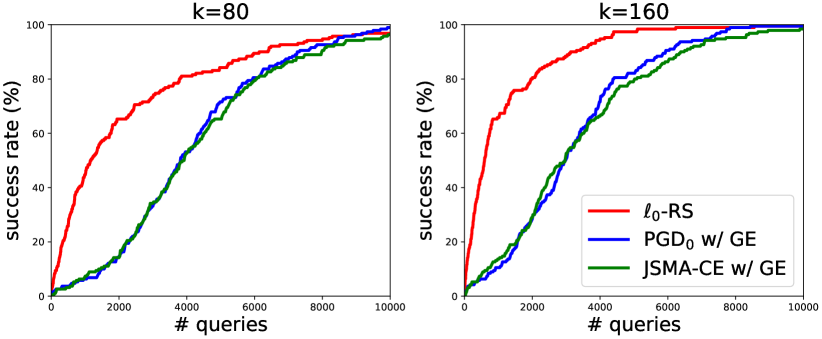
Figure 8: Success rate vs number of queries in fooling a malware detector for sparsity levels $k\in\{80,160\}$. $l_{0}$-RS outperforms the competitors, with a large gap in the low query regime.

Results. We compare the attacks allowed to modify $k\in\{80,160\}$ features and with a maximum of $10000$ queries. Fig. 8 shows the progression of success rate (computed on the initially correctly classified apps) of the attacks over number of queries used. At both sparsity levels, our $l_{0}$-RS attack (in red) achieves very high success rate and outperforms JSMA (green) and PGD₀ (blue) in the low query regime, where the approximation of the gradient is likely not sufficiently precise to identify the most relevant feature for the attacker to perturb.

input : cross-entropy loss $L$, input point $x_{\textrm{orig}}{}$, number of iterations $N$, pixel budget $k$, number of iterations for gradient estimation $m$, gradient estimation step size $\eta$

output : $z$

1 $g\leftarrow\mathbf{0}$,  $q\leftarrow 2\cdot m$

2 while $q\leq N$ do

3       $g\leftarrow\texttt{GradEst}(L,x_{\textrm{orig}},m,\eta,g)$

4       $z\leftarrow x_{\textrm{orig}}{}$

5       $A\leftarrow$ indices of $k$ largest positive components of $g$ (if there are)

6       $z_{A}\leftarrow 1$

7       $q\leftarrow q+2\cdot m$

8       if $z$ is adversarial then return;

9      

Algorithm 3 JSMA-CE with gradient estimation (malware detection)

B.1 Competitors

JSMA-CE with gradient estimation. The idea of the white-box attack of (Grosse et al. 2016) is, given a sparsity level of $k$, to perturb iteratively the feature of the iterate $x^{(i)}$ which corresponds to the largest value (if positive) of $\nabla_{x}L_{\text{CE}}(f(x^{(i)}),y)$, with $f$ the classifier, $y$ the correct label and $L_{\text{CE}}$ the cross-entropy loss, until either the maximum number of modifications are made or misclassification is achieved. With only approximate gradients this approach is not particularly effective. However, since $k\ll d$ and only additions can be made, we aim at estimating the gradient of the cross-entropy loss at $x_{\textrm{orig}}{}$ and then set to 1 the $k$ elements (originally 0) of $x_{\textrm{orig}}{}$ with the largest component in the approximated gradient. With the goal of query efficiency, every $m$ iterations of gradient estimation through finite differences we check if an adversarial example has been found (we do not count these queries in the total for the query limit). Alg. 3 shows the procedure, and we set $m=5$ and $\eta=1$ (we tested other values which achieved worse or similar performance).

PGD₀ with gradient estimation. We use PGD₀ with the gradient estimation technique presented in Alg. 2 with the original point as input $x$, $m=10$, $\eta=100$ and the current estimate of the gradient as prior $p$ (unlike on image classification tasks where the gradient is estimated at the current iterate and no prior used). Moreover, we use step size $4\cdot\sqrt{d}$ and modify the projection step the binary input case and so that features are only added and not removed (see above).

Appendix C Image- and location-specific adversarial patches

We here report the details of the attacks for image- and location-specific adversarial patches.

C.1 Patch-RS algorithm

As mentioned in Sec. 4.3, in this scenario we optimize via random search the attacks for each image independently. In Patch-RS we alternate iterations where a candidate update of the patch is sampled with others where a new location is sampled.

Location updates. We have a location update every $m$ iterations, with $m=5$ ($1:4$ scheme Sec. G.2, four patch updates then one location update) for untargeted attacks and $m=10$ for targeted ones: the latter have more queries available (50k vs 10k) and wider patches ($40\times 40$ vs $20\times 20$), therefore it is natural to dedicate a larger fraction of iterations to optimizing the content rather than the position (which has also a smaller feasible set). We present in Sec. G.2 an ablation study the effect of different frequencies of location updates in the untargeted scenario. The position of the patch is updated with an uniformly sampled shift in $[-h^{(i)},h^{(i)}]$ for each direction (plus clipping to the image size if necessary), where $h^{(i)}$ is linearly decreased from $h^{(0)}=0.75\cdot s_{\text{image}}$ to $h^{(N)}=0$ ($s_{\text{image}}$ indicates the side of the squared images). In this way, initially, the patch can be easily moved on the image, while towards the final iterations it is kept (almost) fixed and only its values are optimized.

Patch updates. The patch is initialized by superposing at random positions on a black image 1000 squares of random size and color in $\{0,1\}^{3}$. Then, we update the patch following the scheme of Square Attack (Andriushchenko et al. 2020), that is sampling random squares with color one of the corners of the color cube and accept the candidate if it improves the target loss. The size of the squares is decided by a piecewise constant schedule, which we inherit from (Andriushchenko et al. 2020). Specifically, at iteration $i$ the square-shaped updates of a patch with size $s\times s$ have side length $s^{(i)}=\sqrt{\alpha^{(i)}}\cdot s$, where the value of $\alpha^{(i)}$ starts with $\alpha^{(0)}=\alpha_{\text{init}}$ and then is halved at iteration $j\in\{10,50,200,500,1000,2000,4000,6000,8000\}$ if the query limit is $N=10,000$, otherwise the values of $j$ are linearly rescaled according to the new $N$. Hence, $\alpha_{\text{init}}$ is the only tunable parameters of Patch-RS, and we set $\alpha_{\text{init}}=0.4$ for untargeted attacks and $\alpha_{\text{init}}=0.1$ for targeted ones.

In contrast to Square Attack, in the second half of the iterations dedicated to updates of size $1\times 1$, Patch-RS performs a refinement of the patch applying only single-channel updates. We show in Sec. G.2 that both the initialization tailored for the specific threat model and the single-channel updates allow our algorithm to achieve the best success rate and query efficiency.

C.2 Competitors

Sparse-RS + SH and Sparse-RS + SA. When integrating SignHunter (Al-Dujaili and O’Reilly 2020) and Square Attack (Andriushchenko et al. 2020) in our framework for adversarial patches, the updates of the locations are performed as described above, while the patches are modified with the $l_{\infty}$ attacks with constraints given by the input domain $[0,1]^{d}$ (in practice one can fix a sufficiently large $l_{\infty}$ threshold $\epsilon_{\infty}=1$). SH does not have free parameters, while we tune the only parameter $p$ of SA (which has the same role as $\alpha_{\text{init}}$ of Patch-RS) and use $p=0.4$ and $p=0.2$ for the untargeted and targeted case respectively.

LOAP. Location-Optimized Adversarial Patches (LOAP) (Rao, Stutz, and Schiele 2020) is a white-box PGD-based attack which iteratively first updates the patch with a step in the direction of the sign of the gradient to maximize the cross-entropy function at the current iterate, then it tests if shifting of stride pixels the patch in one of the four possible directions improves the loss and, if so, the location is updated otherwise kept ((Rao, Stutz, and Schiele 2020) have also a version where only one random shift is tested). We use LOAP as implemented in https://github.com/sukrutrao/Adversarial-Patch-Training with 1,000 iterations, learning rate 0.05 and the full optimization of the location with stride=5. To adapt LOAP to the black-box setup, we use the gradient estimation via finite differences shown in Alg. 2 restricted to the patch to optimize (this means that the noise sampled in step 3 is applied only on the components of the image where the patch is). In particular we use the current iterate as input $x$, $m=5$ iterations, $\eta=10/(s\cdot\sqrt{c})$ if the patch has dimension $s\times s\times c$ and the gradient estimation at the previous iteration as prior $p$. Moreover, we perform the update of the location by sampling only 1 out of the 4 possible directions (as more queries are necessary for better gradient estimation) with stride=5, and learning rate 0.02 for the gradient steps (the sign of the gradient is used as a direction). Note that we optimized these hyperparameters to achieve the best final success rate. Moreover, each iteration costs 11 queries (10 for Alg. 2 and 1 for location updates) and we iterate the procedure until the budget of queries is exhausted.

TPA. The second method we compare to is TPA (Yang et al. 2020), which is based on reinforcement learning and exploits a dictionary of patches. Note that in (Yang et al. 2020) TPA was used primarily putting multiple patches on the same image to achieve misclassification, while our threat model does not include this option. We obtained the optimal values for the hyperparameters for untargeted attacks (rl_batch=400 and steps=25) via personal communication with the authors and set those for the targeted scenario (rl_batch=1000 and steps=50) similarly to what reported in the original code at https://github.com/Chenglin-Yang/PatchAttack, doubling the value of rl_batch to match the budget of queries we allow. TPA has a mechanism of early stopping, which means that it might happen that not the whole budget of queries is exploited even for unsuccessful points. Finally, (Yang et al. 2020) show that TPA significantly outperforms the methods of (Fawzi and Frossard 2016), which also generates image-specific patches, although optimizing the shape and the location but not the values of the perturbation. Thus we do not compare directly to (Fawzi and Frossard 2016) in our experiments.

Appendix D Image-specific adversarial frames

Adversarial frames introduced in (Zajac et al. 2019) are another sparse threat model where the attacker is allowed to perturb only pixels along the borders of the image. In this way, the total number of pixels available for the attack is small (3%-5% in our experiments), and in particular the semantic content of the image is not altered by covering features of the correct class. Thus, this threat model shows how even peripheral changes can influence the classification.

		attack	VGG			ResNet
			success rate	mean queries	med. queries	success rate	mean queries	med. queries
untarget. (2 px wide)	black-box	AF w/ GE	57.6% $\pm$ 0.4	5599 $\pm$ 23	6747 $\pm$ 127	70.6% $\pm$ 0.7	4568 $\pm$ 13	3003 $\pm$ 116
		Sparse-RS + SH	79.9%	3169	882	88.7%	2810	964
		Sparse-RS + SA	77.8% $\pm$ 2.0	3391 $\pm$ 215	1292 $\pm$ 220	80.7% $\pm$ 1.4	3073 $\pm$ 111	1039 $\pm$ 93
		Frame-RS	90.2% $\pm$ 0.3	2366 $\pm$ 26	763 $\pm$ 32	94.0% $\pm$ 0.3	1992 $\pm$ 34	588 $\pm$ 10
2-9		White-box AF	100%	-	-	100%	-	-
targeted (3 px wide)	black-box	AF w/ GE	16.1% $\pm$ 1.5	45536 $\pm$ 328	50000 $\pm$ 0	40.6% $\pm$ 1.4	39753 $\pm$ 459	50000 $\pm$ 0
		Sparse-RS + SH	52.0%	32223	41699	73.2%	25929	20998
		Sparse-RS + SA	32.9% $\pm$ 1.9	38463 $\pm$ 870	50000 $\pm$ 0	47.5% $\pm$2.8	33321 $\pm$ 980	48439 $\pm$ 3500
		Frame-RS	65.7% $\pm$ 0.4	28182 $\pm$ 99	27590 $\pm$ 580	88.0% $\pm$ 0.9	19828 $\pm$ 130	15325 $\pm$370
2-9		White-box AF	100%	-	-	100%	-	-

Table 8: Success rate and query statistics of image-specific frames computed for 5 seeds. Black-box attacks are given 10k/50k queries for untargeted/targeted case. SH is a deterministic method. Frame-RS achieves the best success rate and efficiency in all settings.

Untargeted frames			Targeted frames
Lens cap $\rightarrow$ Chain	Rugby ball $\rightarrow$ Bottle cap	Blue heron $\rightarrow$ Pole	Collie $\rightarrow$ Canoe	Lakeside $\rightarrow$ Tiger	Bullterrier $\rightarrow$ Website

Figure 9: Image-specific untargeted (2 pixels wide) and targeted (3 pixels) frames generated by our Frame-RS algorithm.

D.1 General algorithm for frames

Unlike patches (Sec. 5), for frames the set of pixels $M$ which can be perturbed (see Alg. 1) is fixed. However, similarly to patches, the pixels of the frame can be changed arbitrarily in $[0,1]^{3}$ and thus we can use $l_{\infty}$-black-box attacks for step 7 in Alg. 1 which we denote as Sparse-RS + SH and Sparse-RS + SA. While SH is agnostic to the shape of the perturbations defined by adversarial frames and can be successfully applied for step 7 without further modifications, Sparse-RS + SA leads to suboptimal performance (see Table 8). Indeed, in the frame setting, the sampling distribution of SA requires its square updates to be entirely contained in the frame which due to its small width strongly limits the potential updates. Thus, to achieve better performance, we propose a new sampling distribution specific to frames which, combined with Sparse-RS framework, we call Frame-RS.

D.2 Frames-RS algorithm

Our new sampling distribution (used for step 7 of Alg. 1) returns squares that only partially overlap with the frame. Effectively, we have more flexible updates, often of non-squared shape. Moreover, similarly to Patch-RS, we introduce single-channel updates in the final phase. We also use a different initialization in step 2: uniformly random sampling instead of vertical stripes. As a result, Frame-RS shows significantly better results than both Sparse-RS + SH and Sparse-RS + SA.

We initialize the components of the frame with random values in $\{0,1\}$. Then, at each iteration $i$ we sample uniformly a pixel of the frame to be a random corner of a square of size $s^{(i)}\times s^{(i)}$: all the pixels in the intersection of such square with the frame are set to the same randomly chosen color in $\{0,1\}^{c}$ to create the candidate update. The length of the side of the square is regulated by a linearly decreasing schedule ($s^{(i)}=3\lceil\alpha_{\text{init}}\cdot w^{2}\cdot(0.5-i/N)\rceil$, with $N$ the total number of queries available and $w$ the width of the frame) for the first 50% of queries, after which $s^{(i)}=1$. Finally, for the last 75% of iterations, only single-channel updates are performed. Similarly to the other threat models, the only hyperparameter is $\alpha_{\text{init}}$.

D.3 Competitors

Sparse-RS + SH and Sparse-RS + SA. SignHunter can be directly used to generate adversarial frames as this method does not require a particular shape of the perturbation set. Square Attack is specifically designed for rectangular images and we adapted it to this setting by constraining the sampled updates to lay inside the frame, as they are contained in the image for the $l_{\infty}$- and $l_{2}$- threat models. Since the perturbation set has a different shape than in the other threat models a new schedule for the size of squares specific for this case: at iteration $i$ of $N$ and with frames of width $w$, we have $s^{(i)}=\lceil\alpha_{\text{init}}\cdot w\cdot(0.5-i/N)\rceil$ until $i<N/2$, then $s^{(i)}=1$ (we set $\alpha_{\text{init}}=2$).

Adversarial framing (AF). In (Zajac et al. 2019) propose a method based on gradient descent to craft universal adversarial frames. We here use standard PGD on the cross-entropy loss to generate image-specific perturbations by updating only the components corresponding to the pixels belonging to the frame. In details, we use 1000 iterations with step size 0.05 using the sign of the gradient as direction and each element is projected on the interval $[0,1]$. This white-box attack achieves 100% of success in all settings we tested (consider that 1176 and 2652 pixels be perturbed for the untargeted and targeted scenarios respectively). For the black-box version, we use the gradient estimation technique as for patches (Sec. C), that is Alg. 2 with the current iterate as input $x$, $m=5$, $\eta=10/\sqrt{d}$ and the gradient estimated at the previous iteration as prior $p$, where $d$ represents the number of features in the frame. Moreover, we use step size 0.1 for the untargeted case, 0.01 for the targeted one. Note that we found the mentioned values via grid search to optimize the success rate. We iterate the procedure, which costs 10 queries of the classifier, until reaching the maximum number of allowed queries or finding a successful adversarial perturbation.

D.4 Experimental evaluation

For untargeted attacks we use frames of width 2 and a maximum of 10,000 queries, and for targeted attacks we use frames of width 3 and maximally 50,000 queries. In Table 8 we show that our Frame-RS achieves the best success rate (at least 10% higher than the closest competitor) and much better query efficiency in all settings. In particular, Frame-RS significantly outperforms Sparse-RS + SA, showing that our new sampling distribution is crucial to obtain an effective attack. For the untargeted case the success rate of our black-box Frame-RS is close to that of the white-box AF method which achieves 100% success rate. Finally we illustrate some examples of the resulting images in Fig. 9.

Appendix E Targeted universal attacks: patches and frames

We here report the additional results and implementation details of the attacks for targeted universal patches and frames.

E.1 Sparse-RS for targeted universal attacks

Targeted universal attacks have to generalize to unseen images and, in the case of patches, random locations on the image. We propose to generate them in a black-box scenario with the following scheme, with a budget of 100k iterations. We select a small batch of training images $\{x_{i}\}_{i=1}^{n}$ ($n=30$) and apply the patch at random positions on them (for frames the location is determined by its width). This positions are kept fixed for 10k iterations during which the patch is updated (step 7 of Alg. 1) with some black-box attack (we use the same as for image-specific attacks in Sec. 5 and Sec. D) to minimize the loss

$$L_{\text{targ}}(\{x_{i}\}_{i=1}^{n})=\sum_{i=1}^{n}L_{\text{CE}}(f(x_{i}),t),$$ (3)

where $t$ is the target class. Then, to foster generalization, we resample both the batch of training images and the locations of the patch over them (step 6 in Alg. 1). In this way it is possible obtain black-box attacks without relying on surrogate models. Note that 30 queries of the classifiers are performed at every iteration of the algorithm.

In this scheme, as mentioned, we integrate either SignHunter or Square Attack to have Sparse-RS + SH and Sparse-RS + SA, and our novel Patch-RS introduced for image-specific attacks. In the case of patches, for Sparse-RS + SA we set $p=0.05$ and for Patch-RS $\alpha_{\text{init}}=0.05$ (recall that both parameters control the schedule for sampling the updates in a similar way for the two attacks, details in Sec. C). For frames, for SA we use the schedule for image-specific attacks (Sec. D) with $\alpha_{\text{init}}=0.7$, while in Frame-RS we adapt the schedule for image-specific attacks to the specific case, so that the size of the squares decrease to $s^{(i)}=1$ at $i=25,000$ and single-channel updates are sampled from $i=62,500$.

E.2 Transfer-based attacks

We evaluate the performance of targeted universal patches and frames generated by PGD (Madry et al. 2018) and MI-FGSM (Dong et al. 2018) on a surrogate model and then transferred to attack the target model. In particular, at every iteration of the attack we apply on the training images (200) the patch at random positions (independently picked for every image), average the gradients of the cross-entropy loss at the patch for all images, and take a step in the direction of the sign of the gradients (we use 1000 iterations, step size of 0.05 and momentum coefficient 1 for MI-FGSM). For patches, we report the success rate as the average over 500 images, 10 random target classes, and 100 random positions of the patches for each image. For frames, we average over 5000 images and the same 10 random target classes. In Table 9 we show the success rate of the transfer based attacks on the surrogate model but with images unseen when generating the perturbation and on the target model (we use VGG and ResNet alternatively as the source and target models). We see that the attacks achieve a very high success rate when applied to new images on the source model, but are not able to generalize to another architecture. We note that (Brown et al. 2017) also report a similarly low success rate for the same size of the patch ($50\times 50$ which corresponds to approximately 5% of the input image, see Fig. 3 in (Brown et al. 2017)) on the target class they consider. Finally, we note that (Dong et al. 2018) show that the perturbations obtained with MI-FGSM have better transferability compared to PGD, while in our experiments they are slightly worse, but we highlight that such observation was done for image-specific $l_{\infty}$- and $l_{2}$-attacks, which are significantly different threat models from what we consider here.

	attack	succ. rate
		V $\rightarrow$ V	V $\rightarrow$ R	R $\rightarrow$ R	R $\rightarrow$ V
patches	PGD	99.6%	0.0%	94.9%	3.3%
	MI-FGSM	99.1%	0.0%	92.6%	1.3%
frames	PGD	99.4%	0.0%	99.8%	0.0%
	MI-FGSM	99.3%	0.0%	99.7%	0.0%

Table 9: Success rate of transfer-based targeted universal patches, with VGG (V) and ResNet (R) used as either source or target model averaged over 10 classes. When source and target model are the same network, the attack is only used on unseen images. These targeted universal attacks are very effective when transferred to unseen images on the source model, but do not generalize to the other architecture.

E.3 Targeted universal attacks via gradient estimation

PGD w/ GE. Consistently with the other threat models, we test a method based on PGD with gradient estimation. In particular, in the scheme introduced in Sec. E.1 for Sparse-RS, we optimize the loss with the PGD attack (Madry et al. 2018) and the gradient estimation technique via finite differences as in Alg. 2, similarly to what is done for image-specific perturbations in Sec. C and Sec. D (we also use the same hyperparameters, step size 0.1 for PGD).

ZO-AdaMM. (Chen et al. 2019) propose a black-box method for universal attacks of minimal $l_{2}$-norm able to fool a batch of images, without testing them on unseen images. We adapt it to the case of patches and frames removing the penalization term in the loss which minimizes the $l_{2}$-norm of the perturbations since it is not necessary in our threat models, and integrate it in our scheme introduced in Sec. E.1. We used the standard parameters and tuned learning rate, setting 0.1 for patches, 0.5 for frames. In particular, 10 random perturbations, each equivalent to one query, of the current universal perturbation are sampled to estimate the gradient at each iterations, recalling that the total budget is 100,000 queries.

attack	patches		frames
	VGG	ResNet	VGG	ResNet
Transfer PGD	3.3%	0.0%	0.0%	0.0%
Transfer MI-FGSM	1.3%	0.0%	0.0%	0.0%
PGD w/ GE	35.1%	15.5%	22.7%	52.4%
ZO-AdaMM	45.8%	6.0%	41.8%	53.5%
Sparse-RS + SH	63.9%	13.8%	48.8%	65.5%
Sparse-RS + SA	72.9% $\pm$ 3.6	29.6% $\pm$ 5.6	43.0% $\pm$ 1.2	63.6% $\pm$ 2.1
Patch-RS / Frame-RS	70.8% $\pm$ 1.3	30.4% $\pm$ 8.0	55.5% $\pm$ 0.3	65.3% $\pm$ 2.3

Table 10: Average success rate of targeted universal attacks over 10 target classes on VGG and ResNet. We use patches of size $50\times 50$ and frames of width $6$ pixels and repeat the attacks based on random search with 3 random seeds.

Targeted universal patches			Targeted universal frames
Sulphur butterfly $\rightarrow$ Rottweiler	Persian cat $\rightarrow$ Slug	Starfish $\rightarrow$ Polecat	African elephant $\rightarrow$ Slug	Projector $\rightarrow$ Colobus (monkey)	Vine snake $\rightarrow$ Butcher shop
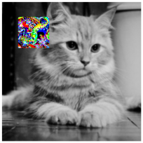
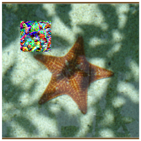
Echidna $\rightarrow$ Rottweiler	Geyser $\rightarrow$ Slug	Electric guitar $\rightarrow$ Polecat	Ballpoint $\rightarrow$ Slug	Grey whale $\rightarrow$ Colobus (monkey)	Beacon $\rightarrow$ Butcher shop

Figure 10: Targeted universal patches and frames generated by our Patch-RS and Frame-RS. We show two images in each column with the same universal patch/frame that is able to change the decision of the classifier into the desired target class.

E.4 Additional results

To evaluate the success of a targeted universal patch, we apply to each of 500 images the patch at 100 random locations and compute the percentage of the perturbed images which are classified in the target class. For targeted universal frames, we compute the success rate applying the perturbation to 5,000 images (unseen during training). The results in Table 5 in Sec. 6 are computed as mentioned above for 10 randomly chosen target classes and then averaged (the same set of target classes is used for patches and frames). For the random search based attacks, we repeat the attacks for 3 random seeds. We report the complete results for both threat models in Table 10. Visualizations of the perturbations found by our scheme are shown in Fig. 10. Finally, we report the details of the success rate on each class in Table 11 for adversarial patches and Table 12 for adversarial frames.

class	VGG			ResNet
	Sparse-RS + SH	Sparse-RS + SA	Patch-RS	Sparse-RS + SH	Sparse-RS + SA	Patch-RS
Rottweiler	61.4%	77.1% $\pm$ 14.6	83.4% $\pm$ 3.9	0.2%	42.6% $\pm$ 26.6	44.4% $\pm$ 29.3
Lakeland terrier	65.4%	86.0% $\pm$ 2.7	76.1% $\pm$ 9.7	0.5%	0.6% $\pm$ 0.2	12.2% $\pm$ 14.8
polecat	46.7%	29.5% $\pm$ 20.6	47.1% $\pm$ 32.3	0.1%	27.3% $\pm$ 15.5	15.0% $\pm$ 9.7
waffle iron	86.3%	82.3% $\pm$ 3.2	74.7% $\pm$ 3.7	17.4%	16.2% $\pm$ 3.9	18.6% $\pm$ 4.9
whippet	37.7%	73.6% $\pm$ 1.6	52.7% $\pm$ 6.0	0.1%	36.9% $\pm$ 24.0	35.4% $\pm$ 24.0
digital clock	97.8%	97.6% $\pm$ 0.2	97.0% $\pm$ 0.5	90.5%	90.4% $\pm$ 3.1	92.5% $\pm$ 1.3
colobus	69.1%	68.9% $\pm$ 5.2	80.1% $\pm$ 4.7	0.0%	0.0% $\pm$ 0.0	0.0% $\pm$ 0.0
slug	61.0%	55.8% $\pm$ 6.9	68.1% $\pm$ 4.8	27.9%	43.7% $\pm$ 1.7	44.2% $\pm$ 10.7
butcher shop	42.4%	67.4% $\pm$ 2.1	44.1% $\pm$ 31.1	1.8%	2.4% $\pm$ 0.6	1.0% $\pm$ 0.5
bluetick	71.3%	90.5% $\pm$ 1.1	85.0% $\pm$ 2.4	0.0%	35.8% $\pm$ 18.5	40.9% $\pm$ 19.5

Table 11: Success rate of targeted universal patches for each of the 10 randomly chosen target classes.

class	VGG			ResNet
	Sparse-RS + SH	Sparse-RS + SA	Frame-RS	Sparse-RS + SH	Sparse-RS + SA	Frame-RS
Rottweiler	39.4%	34.9% $\pm$ 7.5	61.8% $\pm$ 8.5	79.9%	77.6% $\pm$ 4.5	81.6% $\pm$ 8.2
Lakeland terrier	60.3%	45.6% $\pm$ 9.7	69.9% $\pm$ 8.3	81.9%	77.7% $\pm$ 6.5	88.4% $\pm$ 1.7
polecat	13.8%	31.2% $\pm$ 1.5	33.5% $\pm$ 2.8	17.7%	15.1% $\pm$ 6.0	11.2% $\pm$ 9.1
waffle iron	36.0%	35.5% $\pm$ 3.9	49.4% $\pm$ 6.8	81.2%	65.2% $\pm$ 11.4	70.5% $\pm$ 8.0
whippet	63.6%	22.1% $\pm$ 2.4	44.5% $\pm$ 11.1	51.0%	63.4% $\pm$ 9.0	51.5% $\pm$ 2.5
digital clock	95.3%	96.0% $\pm$ 0.2	96.5% $\pm$ 0.7	99.4%	99.6% $\pm$ 0.2	99.8% $\pm$ 0.1
colobus	3.5%	3.9% $\pm$ 2.1	2.5% $\pm$ 0.7	16.8%	0.5% $\pm$ 0.1	4.1% $\pm$ 2.9
slug	51.1%	45.1% $\pm$ 4.7	50.7% $\pm$ 3.5	73.8%	68.1% $\pm$ 6.4	72.5% $\pm$ 6.3
butcher shop	78.9%	67.9% $\pm$ 6.3	83.5% $\pm$ 3.3	92.2%	88.9% $\pm$ 2.5	91.6% $\pm$ 3.9
bluetick	46.2%	48.0% $\pm$ 3.9	65.1% $\pm$ 7.4	61.3%	79.2% $\pm$ 1.9	82.0% $\pm$ 4.2

Table 12: Success rate of targeted universal frames for each of the 10 randomly chosen target classes.

Appendix F Theoretical analysis of $l_{0}$-RS

In this section we prove the following proposition which shows that $l_{0}$-RS requires a sublinear number of queries (improving upon the linear number of queries needed by naive gradient estimation approaches).

Proposition 4.1

The expected number $t_{k}$ of queries needed for $l_{0}$-RS with $\alpha^{(i)}=\nicefrac{{1}}{{k}}$ to find a set of $k$ weights out of the smallest $m$ weights of a linear model is:

$$\mathbb{E}\left[t_{k}\right]=(d-k)k\sum_{i=0}^{k-1}\frac{1}{(k-i)(m-i)}<(d-k)k\frac{\ln(k)+2}{m-k}.$$

Proof. According to the $l_{0}$-RS algorithm, we have $d$ features grouped in a set $U$ and the goal is to find a set $M\subset U$ containing $k$ elements among the $m$ smallest elements of $U$. Since $\alpha^{(i)}=\nicefrac{{1}}{{k}}$, at every iteration we pick one element $p\in M$ to remove from $M$ and one element $q\in U\setminus M$ to add to $M$. This results in a binary vector $z_{new}\in\{0,1\}^{d}$ indicating which are the features in $M$. Then we query the black-box linear model to determine whether the loss at a new point $z_{new}$ improves compared to the point on the previous iteration $z_{current}$, i.e. $L(z_{new})<L(z_{current})$, which gives us information whether $q<p$.

If the current set $M$ contains $i$ elements which belong to the smallest $m$, the probability of increasing it to $i+1$ elements with the next pick is equal to

$$\mathcal{P}[i\rightarrow i+1]= \mathcal{P}[p\notin\text{smallest }m,q\in\text{smallest }m]$$

$$= \frac{k-i}{k}\cdot\frac{m-i}{d-k}.$$

Then the expected number of iterations for the step $i\rightarrow i+1$ is equal to

$$\mathbb{E}[t_{i+1}-t_{i}]=\frac{(d-k)k}{(k-i)(m-i)}$$

since all the draws are independent. Assuming that we begin with none of the smallest $m$ elements in $M$, the expected number of iterations $t_{k}$ needed to find a set of $k$ weights out of the smallest $m$ weights is given by

$$\begin{split}\mathbb{E}[t_{k}]=&\sum_{i=0}^{k-1}\mathbb{E}[t_{i+1}-t_{i}]=\sum_{i=0}^{k-1}\frac{(d-k)k}{(k-i)(m-i)}\\ =&(d-k)k\sum_{i=0}^{k-1}\frac{1}{(k-i)(m-i)}.\end{split}$$ (4)

Now assuming that $m>k$, we can write the summation as:

$$\begin{split}\sum_{i=0}^{k-1}\frac{1}{(k-i)(m-i)}&=\sum_{j=1}^{k}\frac{1}{j(j+m-k)}\\ &=\frac{1}{m-k}\sum_{j=1}^{k}\left(\frac{1}{j}-\frac{1}{j+m-k}\right)\\ &=\frac{1}{m-k}\left(H_{k}-H_{m}+H_{m-k}\right),\end{split}$$ (5)

where $H_{k}$ is the $k$-th harmonic number. Using the fact that $\ln(k)<H_{k}\leq\ln(k)+1$, we have

$$H_{k}-H_{m}+H_{m-k}<\ln(k)-\ln(m)+\ln(m-k)+2$$

and

$$\ln(k)-\ln(m)+\ln(m-k)+2<\ln(k)+2.$$

If we combine this result with Eq. (4) and Eq. (5), we obtain the desired upper bound on $\mathbb{E}\left[t_{k}\right]$:

$$\mathbb{E}\left[t_{k}\right]<(d-k)k\frac{\ln(k)+2}{m-k}.$$

$\square$

Remark F.1

We further remark that for $m=k$ we get that

$$\mathbb{E}[t_{k}]=(d-k)k\sum_{j=1}^{k}\frac{1}{j^{2}}<\frac{\pi^{2}}{6}(d-k)k,$$

however we are interested in the setting when the gap $m-k$ is large enough so that $\mathbb{E}\left[t_{k}\right]$ becomes sublinear.

The main conclusion from Proposition 4.1 is that $\mathbb{E}\left[t_{k}\right]$ becomes sublinear for large enough gap $m-k$ which we further illustrate in Fig. 11 where we plot the expected number of queries needed by $l_{0}$-RS for $d=150,528$ and $k=150$ which is equivalent to our ImageNet experiments with $50$ pixels perturbed.

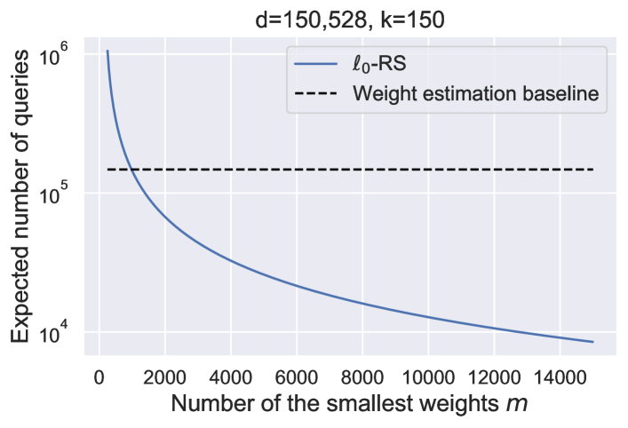
Figure 11: Comparison of the query efficiency of $l_{0}$-RS to that of the naive weight estimation baseline which requires $O(d)$ queries to estimate the gradient.

Appendix G Ablation studies

We here present a series of ablation studies to better understand the robustness of our algorithms to different random seeds, how its performance changes depending on $\alpha_{\text{init}}$, and to justify the algorithmic choice of the piecewise decaying schedule for $\alpha^{(i)}$. We focus the ablation study only on $l_{0}$-RS and Patch-RS methods since for other threat models the setting is less challenging as there is no need to optimize the location of the perturbation.

G.1 $l_{0}$-bounded attacks

Different random seeds. First, we study how the performance of $l_{0}$-RS in the pixel space varies when using different random seeds, which influence the stochastic component inherent in random search. In Table 13 we report mean and standard deviation over 10 runs (with different seeds) of success rate, average and median queries of $l_{0}$-RS on VGG and ResNet with sparsity levels $k\in\{50,100,150\}$ (the same setup of Sec. 4.1, with the additional $k=100$). One can observe that the success rate is very stable in all the cases and the statistics of query consumption consistent across different runs.

model	$k$	success rate (%)	successful points		all points
			avg. queries	med. queries	avg. queries	med. queries
VGG	$50$	$97.4\pm 0.42$	$497\pm 28$	$80\pm 4$	$745\pm 43$	$86\pm 5$
	$100$	$99.8\pm 0.14$	$320\pm 20$	$42\pm 3$	$335\pm 17$	$43\pm 3$
	$150$	$100.0\pm 0.00$	$193\pm 16$	$26\pm 2$	$193\pm 16$	$26\pm 2$
ResNet	$50$	$94.6\pm 0.70$	$686\pm 47$	$135\pm 6$	$1187\pm 48$	$166\pm 11$
	$100$	$99.7\pm 0.15$	$544\pm 36$	$73\pm 5$	$571\pm 26$	$74\pm 5$
	$150$	$100.0\pm 0.00$	$365\pm 19$	$49\pm 3$	$365\pm 19$	$49\pm 3$

Table 13: Mean and standard deviation of the success rate and query efficiency of untargeted $l_{0}$-RS repeated with 10 different random seeds. The success rate and query efficiency are very stable over random seeds.

Different values of $\alpha_{\text{init}}$. Then we analyze the behaviour of our algorithm with different values of $\alpha_{\text{init}}$, since it is the only free hyperparameter of Sparse-RS. Let us recall that it is used to regulate how much $M^{\prime}$ and $\Delta^{\prime}$ differ from $M$ and $\Delta$ respectively in steps 6-7 of Alg. 1 at each iteration. Fig. 12 shows the success rate and query usage (computed on the successful samples) of our untargeted $l_{0}$-bounded attack on VGG at the usual three sparsity levels $k$ for runs with $\alpha_{\text{init}}\in\{0.01,0.05,0.1,0.2,0.3,0.4,0.6,0.8,1\}$ (for our experiments in Sec. 4.1 we use $\alpha_{\text{init}}=0.3$). We observe that the success rate is similar (close to $100\%$) for all the values, with a slight degradation for the largest ones. In order to minimize the queries of the classifier, the runs with $\alpha_{\text{init}}$ between $0.1$ and $0.4$ are comparably good, with small differences in the tradeoff between average and median number of queries.

Constant vs decaying $\alpha^{(i)}$. In order to demonstrate the role of decaying the difference between the candidate updates $M^{\prime}$ and $\Delta^{\prime}$ and the current iterates $M$ and $\Delta$ over iterations (see steps 6-7 of Alg. 1) to achieve good performance, we run our attack with constant $\alpha^{(i)}$ schedule instead of the piecewise constant schedule with decreasing values. We fix $\alpha^{(i)}=c\in[0,1]$ for every $i$ so that for the whole algorithm $M^{\prime}$ and $M$ differ in $\max\{c\cdot k,1\}$ elements. In Fig. 13 we report the results achieved by $c\in\{0,0.05,0.15,0.3,0.5,1\}$ on VGG at $k\in\{50,100,150\}$, together with the baseline (black dashed line) of the standard version of $l_{0}$-RS. One can observe that small constant values $c$ for $\alpha^{(i)}=c$ achieve a high success rate but suffer in query efficiency, in particular computed regarding the median and for larger $k$, while the highest values of $c$ lead to significantly worse success rate (note that average and median queries are computed only on the successful points) than the baseline. These results highlight how important it is to have an initial exploration phase, with a larger step size, and at a later stage a more local optimization.

$k=50$ $k=100$ $k=150$

Figure 12: Ablation study on the influence of $\alpha_{\text{init}}$, the hyperparameter which regulates the size of the updates at each iteration. We show success rate (first column), average (second) and median queries (third) achieved by $l_{0}$-RS on VGG at sparsity levels $k=\{50,100,150\}$. Considering jointly the three statistics values in $[0.1,0.4]$ are preferable for this threat model and schedule.

$k=50$ $k=100$ $k=150$

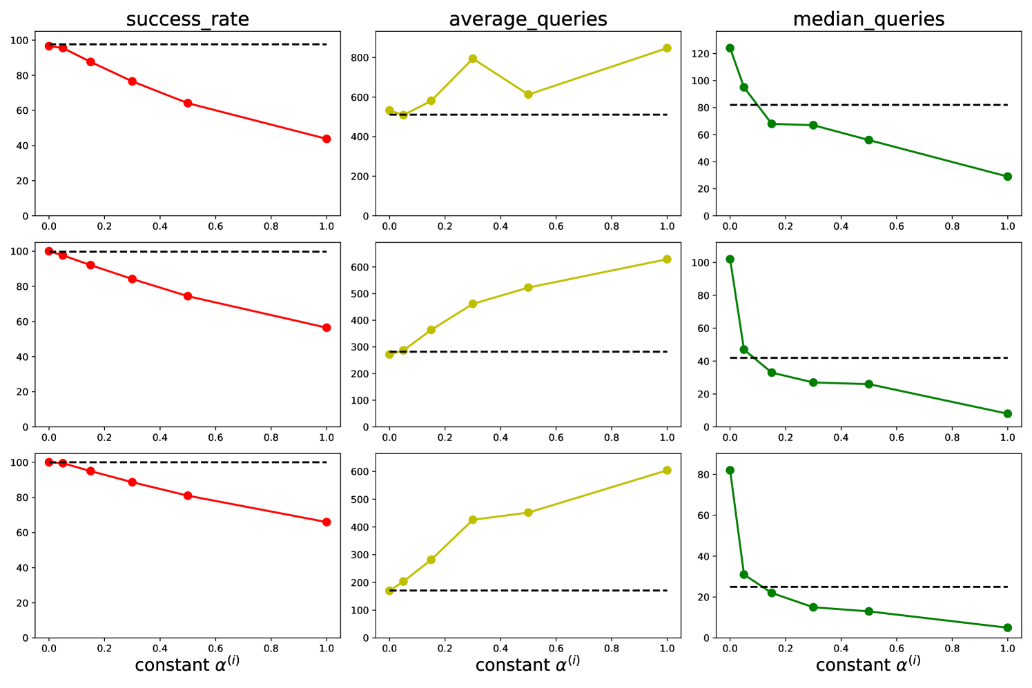
Figure 13: Performance of untargeted $l_{0}$-RS on VGG when using a constant schedule for $\alpha^{(i)}$, that is the size of $|A|=|B|=c\cdot k$ (see Sec. 4) at every iteration, or equivalently $\alpha^{(i)}=c$ for every $i=1,\ldots,N$. The dashed line is the reference of the results achieved with the piecewise constant schedule to decay $\alpha^{(i)}$. While constantly small updates lead to good success rate, the median number of queries used increases notably, especially with larger sparsity levels $k$.

G.2 Image-specific adversarial patches

We here show the individual effect of our algorithmic choices to craft image-specific adversarial patches.

Initialization and single-channel updates.

attack	init.	single	VGG			ResNet
		channel	succ. rate	mean queries	med. queries	succ. rate	mean queries	med. queries
Sparse-RS + SH	-	-	82.6%	2479	514	75.3%	3290	549
Sparse-RS + SA	stripes	no	85.6% $\pm$ 1.1	2367 $\pm$ 83	533 $\pm$ 40	78.5% $\pm$ 1.0	2877 $\pm$ 64	458 $\pm$ 43
	stripes	yes	85.7% $\pm$ 1.4	2359 $\pm$ 89	533 $\pm$ 40	79.1% $\pm$ 1.1	2861 $\pm$ 58	458 $\pm$ 43
	squares	no	87.1% $\pm$ 0.9	2174 $\pm$ 50	429 $\pm$ 22	78.9% $\pm$ 1.3	2820 $\pm$ 91	438 $\pm$ 68
Patch-RS	squares	yes	87.8% $\pm$ 0.7	2160 $\pm$ 44	429 $\pm$ 22	79.5% $\pm$ 1.4	2808 $\pm$ 89	438 $\pm$ 68

Table 14: Ablation study on the effect of initialization and single-channel updates for untargeted image-specific adversarial patches (size $20\times 20$ pixels) within our proposed framework. We highlight in grey our modified schemes that lead to a higher success rate and query efficiency. Note that the single-channel updates come later in the optimization process when 50% success rate is reached, and thus they do not influence the median. We also report the results of Sparse-RS + SH for reference.

The original Square Attack (Andriushchenko et al. 2020) for $l_{\infty}$- and $l_{2}$-bounded perturbations applies as initialization vertical stripes on the target image, and it does not consider updates of a single channel (these can be randomly sampled but are not explicitly performed). Table 14 shows the success rate and query efficiency (computed on all points) for untargeted adversarial attacks with patches of size $20\times 20$ on VGG and ResNet, averaged over 5 random seeds for methods based on random search. Both the initialization with squares and the single-channel updates already individually improve the performance of Sparse-RS + SA and, when combined, allow Patch-RS to outperform the competitors (see also Sec. 4.3).

Ratio location to patch updates.

ratio	attack	VGG			ResNet
location : patch		succ. rate	mean queries	med. queries	succ. rate	mean queries	med. queries
9:1	Sparse-RS + SH	74.9%	3897	1331	68.0%	4038	1121
	Sparse-RS + SA	71.4% $\pm$ 0.9	3927 $\pm$ 104	1361 $\pm$ 224	68.7% $\pm$ 1.0	3931 $\pm$ 76	789 $\pm$ 65
	Patch-RS	76.8% $\pm$ 0.8	3414 $\pm$ 48	779 $\pm$ 69	72.0% $\pm$ 0.8	3655 $\pm$ 57	731 $\pm$ 97
4:1	Sparse-RS + SH	77.1%	3332	781	72.9%	3639	701
	Sparse-RS + SA	77.7% $\pm$ 1.2	3236 $\pm$ 106	735 $\pm$ 41	73.6% $\pm$ 0.6	3408 $\pm$ 35	548 $\pm$ 65
	Patch-RS	82.4% $\pm$ 0.8	2816 $\pm$ 28	485 $\pm$ 74	75.3% $\pm$ 0.5	3248 $\pm$ 51	443 $\pm$ 41
1:1	Sparse-RS + SH	82.9%	2718	500	75.3%	3168	451
	Sparse-RS + SA	84.6% $\pm$ 1.2	2485 $\pm$ 92	504 $\pm$ 20	78.2% $\pm$ 0.7	2943 $\pm$ 142	389 $\pm$ 46
	Patch-RS	86.8% $\pm$ 0.8	2301 $\pm$ 61	352 $\pm$ 28	79.6% $\pm$ 1.1	2764 $\pm$ 86	316 $\pm$ 10
1:4	Sparse-RS + SH	82.6%	2479	514	75.3%	3290	549
	Sparse-RS + SA	85.6% $\pm$ 1.1	2367 $\pm$ 83	533 $\pm$ 40	78.5% $\pm$ 1.0	2877 $\pm$ 64	458 $\pm$ 43
	Patch-RS	87.8% $\pm$ 0.7	2160 $\pm$ 44	429 $\pm$ 22	79.5% $\pm$ 1.4	2808 $\pm$ 89	438 $\pm$ 68
1:9	Sparse-RS + SH	80.7%	2719	564	72.2%	3451	843
	Sparse-RS + SA	85.9% $\pm$ 0.8	2419 $\pm$ 60	542 $\pm$ 34	77.6% $\pm$ 0.8	3000 $\pm$ 92	617 $\pm$ 41
	Patch-RS	87.5% $\pm$ 1.6	2261 $\pm$ 44	542 $\pm$ 39	78.4% $\pm$ 0.6	2961 $\pm$ 34	533 $\pm$ 54

Table 15: Performance of different attacks for untargeted image-specific adversarial patches of size $20\times 20$ varying the ratio between updates of the location and of the patch. We use 1:4 ratio in our framework which is the best choice for Sparse-RS + SA and Patch-RS (for Sparse-RS + SH 1:1 would work equally well). Note that our novel attack Patch-RS outperforms the competitors consistently in terms of the success rate and query efficiency across all choices of the ratio of the location and patch updates. For random search based methods, we repeat the attack with 5 random seeds.

We study here the effect of different ratios between the number of location and patch updates in our framework for image-specific untargeted patches (size $20\times 20$). In Table 15 we report the performance Sparse-RS + SH, Sparse-RS + SA and our final method Patch-RS with various schemes: alternating an update of the location to one of the patch (1:1), doing 4 or 9 location updates for one patch update (4:1, 9:1) and vice versa (1:4, 1:9). Considering the results on both networks, the scheme with 1:4 ratio yields for every attack the highest success rate or very close. In query consumption, the schemes 1:1 and 1:4 are similar, with some trade-off between average and median. Moreover, we observe that the ranking of the three methods is preserved for all ratios of location and patch updates we tested, with Patch-RS outperforming the others. Also, its effectiveness is less affected by suboptimal ratios, showing the stability of our algorithm.

References

- Al-Dujaili et al. (2018) Al-Dujaili, A.; Huang, A.; Hemberg, E.; and O’Reilly, U.-M. 2018. Adversarial deep learning for robust detection of binary encoded malware. In IEEE S&P Workshops, 76–82.
- Al-Dujaili and O’Reilly (2020) Al-Dujaili, A.; and O’Reilly, U.-M. 2020. There are No Bit Parts for Sign Bits in Black-Box Attacks. In ICLR.
- Alzantot et al. (2019) Alzantot, M.; Sharma, Y.; Chakraborty, S.; and Srivastava, M. 2019. Genattack: practical black-box attacks with gradient-free optimization. In GECCO.
- Andriushchenko et al. (2020) Andriushchenko, M.; Croce, F.; Flammarion, N.; and Hein, M. 2020. Square Attack: a query-efficient black-box adversarial attack via random search. In ECCV.
- Arora et al. (2018) Arora, R.; Basuy, A.; Mianjyz, P.; and Mukherjee, A. 2018. Understanding deep neural networks with rectified linear unit. In ICLR.
- Arp et al. (2014) Arp, D.; Spreitzenbarth, M.; Hubner, M.; Gascon, H.; Rieck, K.; and Siemens, C. 2014. Drebin: Effective and explainable detection of android malware in your pocket. In NDSS, volume 14, 23–26.
- Athalye, Carlini, and Wagner (2018) Athalye, A.; Carlini, N.; and Wagner, D. A. 2018. Obfuscated Gradients Give a False Sense of Security: Circumventing Defenses to Adversarial Examples. In ICML.
- Bhagoji et al. (2018) Bhagoji, A. N.; He, W.; Li, B.; and Song, D. 2018. Practical black-box attacks on deep neural networks using efficient query mechanisms. In ECCV.
- Biggio et al. (2013) Biggio, B.; Corona, I.; Maiorca, D.; Nelson, B.; Srndic, N.; Laskov, P.; Giacinto, G.; and Roli, F. 2013. Evasion Attacks against Machine Learning at Test Time. In ECML/PKKD.
- Brendel, Rauber, and Bethge (2018) Brendel, W.; Rauber, J.; and Bethge, M. 2018. Decision-Based Adversarial Attacks: Reliable Attacks Against Black-Box Machine Learning Models. In ICLR.
- Brown et al. (2017) Brown, T. B.; Mané, D.; Roy, A.; Abadi, M.; and Gilmer, J. 2017. Adversarial Patch. In NeurIPS 2017 Workshop on Machine Learning and Computer Security.
- Brunner et al. (2019) Brunner, T.; Diehl, F.; Le, M. T.; and Knoll, A. 2019. Guessing smart: biased sampling for efficient black-box adversarial attacks. In ICCV.
- Carlini and Wagner (2017) Carlini, N.; and Wagner, D. 2017. Towards Evaluating the Robustness of Neural Networks. In IEEE Symposium on Security and Privacy.
- Césaire et al. (2020) Césaire, M.; Hajri, H.; Lamprier, S.; and Gallinari, P. 2020. Stochastic sparse adversarial attacks. arXiv preprint arXiv:2011.12423.
- Chen et al. (2018) Chen, P.; Sharma, Y.; Zhang, H.; Yi, J.; and Hsieh, C. 2018. EAD: Elastic-Net Attacks to Deep Neural Networks via Adversarial Examples. In AAAI.
- Chen et al. (2019) Chen, X.; Liu, S.; Xu, K.; Li, X.; Lin, X.; Hong, M.; and Cox, D. 2019. ZO-AdaMM: Zeroth-order adaptive momentum method for black-box optimization. In NeurIPS.
- Cheng et al. (2019) Cheng, S.; Dong, Y.; Pang, T.; Su, H.; and Zhu, J. 2019. Improving Black-box Adversarial Attacks with a Transfer-based Prior. In NeurIPS.
- Croce et al. (2020) Croce, F.; Andriushchenko, M.; Sehwag, V.; Debenedetti, E.; Flammarion, N.; Chiang, M.; Mittal, P.; and Hein, M. 2020. RobustBench: a standardized adversarial robustness benchmark. arXiv preprint arXiv:2010.09670.
- Croce and Hein (2019) Croce, F.; and Hein, M. 2019. Sparse and Imperceivable Adversarial Attacks. In ICCV.
- Croce and Hein (2020) Croce, F.; and Hein, M. 2020. Minimally distorted Adversarial Examples with a Fast Adaptive Boundary Attack. In ICML.
- Croce and Hein (2021) Croce, F.; and Hein, M. 2021. Mind the box: -APGD for sparse adversarial attacks on image classifiers. In ICML.
- Dong et al. (2018) Dong, Y.; Liao, F.; Pang, T.; Su, H.; Zhu, J.; Hu, X.; and Li, J. 2018. Boosting Adversarial Attacks With Momentum. In CVPR.
- Fan et al. (2020) Fan, Y.; Wu, B.; Li, T.; Zhang, Y.; Li, M.; Li, Z.; and Yang, Y. 2020. Sparse adversarial attack via perturbation factorization. In ECCV.
- Fawzi and Frossard (2016) Fawzi, A.; and Frossard, P. 2016. Measuring the effect of nuisance variables on classifiers. In BMVC.
- Grosse et al. (2016) Grosse, K.; Papernot, N.; Manoharan, P.; Backes, M.; and McDaniel, P. 2016. Adversarial perturbations against deep neural networks for malware classification. arXiv preprint arXiv:1606.04435.
- Guo et al. (2019) Guo, C.; Gardner, J. R.; You, Y.; Wilson, A. G.; and Weinberger, K. Q. 2019. Simple black-box adversarial attacks. In ICML.
- Hu et al. (2020) Hu, J. E.; Swaminathan, A.; Salman, H.; and Yang, G. 2020. Improved Image Wasserstein Attacks and Defenses. arXiv preprint arXiv:2004.12478.
- Hu and Tan (2017) Hu, W.; and Tan, Y. 2017. Generating adversarial malware examples for black-box attacks based on GAN. arXiv preprint arXiv:1702.05983.
- Huang and Zhang (2020) Huang, Z.; and Zhang, T. 2020. Black-Box Adversarial Attack with Transferable Model-based Embedding. In ICLR.
- Ilyas et al. (2018) Ilyas, A.; Engstrom, L.; Athalye, A.; and Lin, J. 2018. Black-box adversarial attacks with limited queries and information. In ICML.
- Ilyas, Engstrom, and Madry (2019) Ilyas, A.; Engstrom, L.; and Madry, A. 2019. Prior convictions: Black-box adversarial attacks with bandits and priors. In ICLR.
- Jin et al. (2019) Jin, D.; Jin, Z.; Zhou, J. T.; and Szolovits, P. 2019. Is BERT Really Robust? Natural Language Attack on Text Classification and Entailment. In AAAI.
- Karmon, Zoran, and Goldberg (2018) Karmon, D.; Zoran, D.; and Goldberg, Y. 2018. Lavan: Localized and visible adversarial noise. In ICML.
- Kurakin, Goodfellow, and Bengio (2017) Kurakin, A.; Goodfellow, I. J.; and Bengio, S. 2017. Adversarial examples in the physical world. In ICLR Workshop.
- Laidlaw, Singla, and Feizi (2021) Laidlaw, C.; Singla, S.; and Feizi, S. 2021. Perceptual Adversarial Robustness: Defense Against Unseen Threat Models. In ICLR.
- Lee and Kolter (2019) Lee, M.; and Kolter, Z. 2019. On physical adversarial patches for object detection. ICML Workshop on Security and Privacy of Machine Learning.
- Li, Schmidt, and Kolter (2019) Li, J.; Schmidt, F.; and Kolter, Z. 2019. Adversarial camera stickers: A physical camera-based attack on deep learning systems. In ICML, 3896–3904.
- Liu et al. (2019) Liu, X.; Du, X.; Zhang, X.; Zhu, Q.; Wang, H.; and Guizani, M. 2019. Adversarial samples on android malware detection systems for IoT systems. Sensors, 19(4): 974.
- Madry et al. (2018) Madry, A.; Makelov, A.; Schmidt, L.; Tsipras, D.; and Valdu, A. 2018. Towards Deep Learning Models Resistant to Adversarial Attacks. In ICLR.
- Matyasko and Chau (2021) Matyasko, A.; and Chau, L.-P. 2021. PDPGD: Primal-Dual Proximal Gradient Descent Adversarial Attack. arXiv preprint arXiv:2106.01538.
- Meunier, Atif, and Teytaud (2019) Meunier, L.; Atif, J.; and Teytaud, O. 2019. Yet another but more efficient black-box adversarial attack: tiling and evolution strategies. arXiv preprint, arXiv:1910.02244.
- Modas, Moosavi-Dezfooli, and Frossard (2019) Modas, A.; Moosavi-Dezfooli, S.; and Frossard, P. 2019. SparseFool: a few pixels make a big difference. In CVPR.
- Moon, An, and Song (2019) Moon, S.; An, G.; and Song, H. O. 2019. Parsimonious Black-Box Adversarial Attacks via Efficient Combinatorial Optimization. In ICML.
- Moosavi-Dezfooli, Fawzi, and Frossard (2016) Moosavi-Dezfooli, S.-M.; Fawzi, A.; and Frossard, P. 2016. DeepFool: a simple and accurate method to fool deep neural networks. In CVPR, 2574–2582.
- Narodytska and Kasiviswanathan (2017) Narodytska, N.; and Kasiviswanathan, S. 2017. Simple black-box adversarial attacks on deep neural networks. In CVPR Workshops.
- Papernot et al. (2016) Papernot, N.; McDaniel, P.; Jha, S.; Fredrikson, M.; Celik, Z. B.; and Swami, A. 2016. The limitations of deep learning in adversarial settings. In 2016 IEEE European symposium on security and privacy (EuroS&P), 372–387. IEEE.
- Pintor et al. (2021) Pintor, M.; Roli, F.; Brendel, W.; and Biggio, B. 2021. Fast Minimum-norm Adversarial Attacks through Adaptive Norm Constraints. arXiv preprint arXiv:2102.12827.
- Podschwadt and Takabi (2019) Podschwadt, R.; and Takabi, H. 2019. On Effectiveness of Adversarial Examples and Defenses for Malware Classification. In International Conference on Security and Privacy in Communication Systems, 380–393. Springer.
- Pooladian et al. (2020) Pooladian, A.-A.; Finlay, C.; Hoheisel, T.; and Oberman, A. M. 2020. A principled approach for generating adversarial images under non-smooth dissimilarity metrics. In AISTATS.
- Rao, Stutz, and Schiele (2020) Rao, S.; Stutz, D.; and Schiele, B. 2020. Adversarial Training against Location-Optimized Adversarial Patches. In ECCV Workshop on the Dark and Bright Sides of Computer Vision: Challenges and Oppurtinities for Privacy and Security.
- Rastrigin (1963) Rastrigin, L. 1963. The convergence of the random search method in the extremal control of a many parameter system. Automaton & Remote Control, 24: 1337–1342.
- Rauber, Brendel, and Bethge (2017) Rauber, J.; Brendel, W.; and Bethge, M. 2017. Foolbox: A Python toolbox to benchmark the robustness of machine learning models. In ICML Reliable Machine Learning in the Wild Workshop.
- Rebuffi et al. (2021) Rebuffi, S.-A.; Gowal, S.; Calian, D. A.; Stimberg, F.; Wiles, O.; and Mann, T. 2021. Fixing data augmentation to improve adversarial robustness. arXiv preprint arXiv:2103.01946.
- Rony and Ben Ayed (2020) Rony, J.; and Ben Ayed, I. 2020. Adversarial Library.
- Rony et al. (2019) Rony, J.; Hafemann, L. G.; Oliveira, L. S.; Ayed, I. B.; Sabourin, R.; and Granger, E. 2019. Decoupling direction and norm for efficient gradient-based l2 adversarial attacks and defenses. In CVPR, 4322–4330.
- Schott et al. (2019) Schott, L.; Rauber, J.; Bethge, M.; and Brendel, W. 2019. Towards the first adversarially robust neural network model on MNIST. In ICLR.
- Stokes et al. (2017) Stokes, J. W.; Wang, D.; Marinescu, M.; Marino, M.; and Bussone, B. 2017. Attack and defense of dynamic analysis-based, adversarial neural malware classification models. arXiv preprint arXiv:1712.05919.
- Szegedy et al. (2014) Szegedy, C.; Zaremba, W.; Sutskever, I.; Bruna, J.; Erhan, D.; Goodfellow, I.; and Fergus, R. 2014. Intriguing properties of neural networks. In ICLR, 2503–2511.
- Thys, Van Ranst, and Goedemé (2019) Thys, S.; Van Ranst, W.; and Goedemé, T. 2019. Fooling automated surveillance cameras: adversarial patches to attack person detection. In CVPR Workshops.
- Tu et al. (2019) Tu, C.-C.; Ting, P.; Chen, P.-Y.; Liu, S.; Zhang, H.; Yi, J.; Hsieh, C.-J.; and Cheng, S.-M. 2019. Autozoom: Autoencoder-based zeroth order optimization method for attacking black-box neural networks. In AAAI.
- Uesato et al. (2018) Uesato, J.; O’Donoghue, B.; Van den Oord, A.; and Kohli, P. 2018. Adversarial risk and the dangers of evaluating against weak attacks. In ICML.
- Wong, Schmidt, and Kolter (2019) Wong, E.; Schmidt, F. R.; and Kolter, J. Z. 2019. Wasserstein Adversarial Examples via Projected Sinkhorn Iterations. In ICML.
- Yang et al. (2020) Yang, C.; Kortylewski, A.; Xie, C.; Cao, Y.; and Yuille, A. 2020. PatchAttack: A Black-box Texture-based Attack with Reinforcement Learning. In ECCV.
- Zabinsky (2010) Zabinsky, Z. B. 2010. Random search algorithms. Wiley encyclopedia of operations research and management science.
- Zajac et al. (2019) Zajac, M.; Zołna, K.; Rostamzadeh, N.; and Pinheiro, P. O. 2019. Adversarial framing for image and video classification. In AAAI, 10077–10078.
- Zhang et al. (2018) Zhang, R.; Isola, P.; Efros, A. A.; Shechtman, E.; and Wang, O. 2018. The unreasonable effectiveness of deep features as a perceptual metric. In CVPR, 586–595.
- Zhao et al. (2019) Zhao, P.; Liu, S.; Chen, P.-Y.; Hoang, N.; Xu, K.; Kailkhura, B.; and Lin, X. 2019. On the design of black-box adversarial examples by leveraging gradient-free optimization and operator splitting method. In ICCV, 121–130.