Weak Lensing Skew-Spectrum

Abstract

We introduce the skew-spectrum statistic for weak lensing convergence $\kappa$ maps and test it against state-of-the-art high-resolution all-sky numerical simulations. We perform the analysis as a function of source redshift and smoothing angular scale for individual tomographic bins. We also analyse the cross-correlation between different tomographic bins. We compare the numerical results to fitting-functions used to model the bispectrum of the underlying density field as a function of redshift and scale. We derive a closed form expression for the skew-spectrum for gravity-induced secondary non-Gaussianity. We also compute the skew-spectrum for the projected $\kappa$ inferred from Cosmic Microwave Background (CMB) studies. As opposed to the low redshift case we find the post-Born corrections to be important in the modelling of the skew-spectrum for such studies. We show how the presence of a mask and noise can be incorporated in the estimation of a skew-spectrum.

1 Introduction

Recently completed CMB experiments such as the Planck Surveyor(Planck Collaboration, 2013, 2018), have helped establishing a standard model of cosmology, with the baseline cosmological parameters now known with an unprecedented accuracy. However, many fundamental questions in cosmology remain open. These include the nature of dark matter and dark energy, a possible modification of General Relativity on cosmological scales (Joyce et al., 2014; Clifton et al., 2012) and the nature of neutrinos mass hierarchy(Lesgourgues & Pastor, 2006). Next generation of large scale surveys will provide a massive amount of high-precision data carrying complementary information that can help answer at least some of these questions. Indeed, observational programs of many ongoing as well as future surveys including the surveys e.g., Euclid(Laureijs et al, 2006), CFHTLS, PAN-STARRS, Dark Energy Surveys(Allam et al., 2016), WiggleZ(Drinkwater et al., 2010), Rubin Observatory,(Tyson et al., 2003), BOSS(Eisenstein et al., 2011), KIDS(Kuijken et al., 2015), Roman Space Telescope(National Research Council, 2010), lists weak lensing as their main science driver. From the early days of detection weak lensing (see e.g. (Munshi et al., 2008) for a review) studies have now reached a level of maturity. Surveys such as Euclid will constrain the cosmological parameters with sub-percent accuracy and answer many of the most challenging questions that cosmology is facing today.

Weak lensing at smaller angular scales probes scales that are in the highly nonlinear regime and contains a wealth of cosmological information. This gravity-induced nonlinearity (Bernardeau et al., 2002) introduces mode-coupling that is responsible for the resulting departure from Gaussianity (Bartolo et al., 2004). Higher-order statistics beyond power spectrum estimation is typically used in exploitation of the information content of weak lensing maps. An accurate modelling of higher-order statistics is important for modelling the covariance of the lower order estimators as well as to break cosmological parameter degeneracy. Early studies of higher-order statistics concentrated on cumulants (Bernardeau, 1994a, b) in real-space (Bernardeau et al., 2002, 2003). Future surveys such as Euclid will have a near all-sky coverage and thus enable quantifying higher-order statistics in the harmonic domain where measurements of individual modes will be less correlated (Amendola et al., 2013).

Most theoretical modelling in the highly nonlinear regime were based on perturbative calculations or its extensions (Bernardeau et al., 2002), variants of the halo models (Cooray & Sheth et al., 2002), Effective Field Theory (Baumann, 2012) or fitting-functions that are calibrated from simulations (Scoccimarro & Frieman, 1999; Gil-Marin et al., 2011). Many different estimators are currently available for analysing departures from Gaussianity, including morphological estimators (Munshi et al., 2012), position-dependent power spectra (Munshi et al., 2019b), line-correlations (Eggemeier & Smith, 2017), extreme value statistics (Harrison & Coles, 2011). peak-statistics (Kacprzak et al., 2016; Shan et al., 2018), void statistics (Krause et al., 2013) and probability distribution functions (Gruen et al., 2018; Uhlemann et al., 2016; Codis et al., 2016; Valageas, 2016).

While measurements of real space correlations are much simpler in the presence of complicated survey boundaries the measurements for different angular scales can be highly correlated (Munshi & Jain, 2001, 2000; Munshi, 2000). In comparison the measurements in the harmonic domain are less correlated and contains independent information if the sky coverage is high. One of the motivation of this study is to develop analytical predictions for one such proxy statistics to the bispectrum called skew-spectrum (Munshi & Heavens, 2010; Cooray, 2001) and test them against state-of-art numerical simulations. We will borrow the concepts developed for constructing skew-spectrum for the the study of non-Gaussianity in the context of Cosmic Microwave Background (CMB) observations by WMAP(Smidt et al., 2010; Calabrese et al., 2018) and Planck(Planck Collaboration, 2015) satellites. However our aim here is also to include gravity induced secondary non-Gaussianity. The skew-spectrum is the lowest-order member in the family of higher-order spectra (Munshi et al., 2011a, b). They can also be used to reconstruct morphological estimators, e.g., Minkowski Functionals, in an order by order manner in the presence of complicated survey topology (Munshi et al., 2012). Recently the skew-spectrum statistics was used to study the possibility of probing galaxy clustering using data from the forthcoming generation of wide-field galaxy surveys(Dai et al., 2019; Schmittfull et al., 2015; Dizgah et al., 2020).

In this paper we show that the skew-spectrum statistics can be used to analyse the weak lensing maps that will be available from the future stage-IV experiments such as Euclid or the Rubin Observatory. We also show how the sub-optimal skew-spectrum can be used to probe the gravity-induced non-Gaussianity of the reconstructed convergence maps from CMB observations. We will present the skew-spectrum by cross-correlating different tomographic bins as well as the CMB convergence maps and the low redshift weak lensing convergence maps. In this context we will emphasize the importance of the post-Born corrections in theoretical modeling of the bispectrum. Finally, we will consider many modified theories of gravity and use second-order perturbation theory to model the theoretical skew-spectrum at large smoothing angular scales to provide an example of important science goals that can be achieved using the skew-spectrum statistics.

This paper is organised as follows. In §2 we briefly review the modelling of the density bispectrum. In §3 we introduce our notations and briefly summarize the results of projected weak lensing convergence or $\kappa$ bispectrum. The §4 is devoted to the discussion of the simulations we use in our study. In §5 we present the estimator we use. The results are discussed in §6 and conclusion and future prospects are presented in §7.

2 Modelling of the Density Bispectrum

In this section we relevant the aspects of tree-level perturbative results and their extensions using approaches based on fitting-function, which we use to compute the bispectrum and eventually the skew-spectrum.

2.1 Tree-level Perturbative Calculations

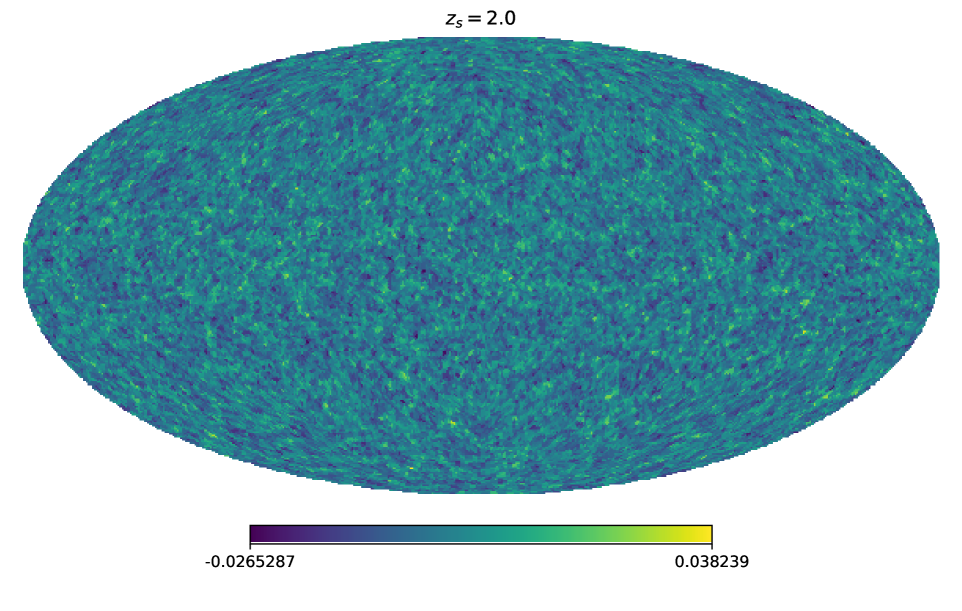
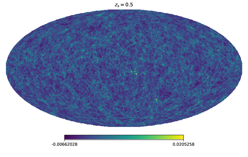
Figure 1: Examples of realisations of all-sky weak lensing convergence or $\kappa$ maps used for our study. The left- and right-panel panels correspond respectively source redshift $z_{s}=2.0$ and $0.5$. The $\kappa$ maps, we have used, were generated at a Healpix resolution $N_{\rm side}=4096$, and we have degraded them to $N_{\rm side}=2048$ for our study.

In the weakly non-linear regime with density contrast ($\delta\leq 1$), the gravitational clustering can be described by the Eulerian perturbation theory Munshi et al. (2008). However, the perturbative treatment eventually breaks down when density contrast at a given length scale becomes nonlinear ($\delta\geq 1$). Expanding the density contrast $\delta$ in a Fourier series, and assuming the density contrast is less than unity, for the pertubative series to be convergent, we get

$$\delta({\bf k})=\delta^{(1)}({\bf k})+\delta^{(2)}({\bf k})+\delta^{(3)}({\bf k})+\dots;$$ (1a)

$$\delta^{(2)}(k)=\int{d^{3}{\bf k}_{1}\over 2\pi}\int{d^{3}{\bf k}_{2}\over 2\pi}\delta_{D}({\bf k_{1}+k_{2}-k})F_{2}({\bf k}_{1},{\bf k}_{2})\delta^{(1)}({\bf k}_{1})\delta^{(1)}({\bf k}_{2});$$ (1b)

$$F_{2}({\bf k}_{1},{\bf k}_{2})={5\over 7}+{1\over 2}\left({k_{1}\over k_{2}}+{k_{2}\over k_{1}}\right)\left({{\bf k}_{1}\cdot{\bf k}_{2}\over k_{1}k_{2}}\right)+{2\over 7}\left({{\bf k}_{1}\cdot{\bf k}_{2}\over k_{1}k_{2}}\right)^{2}.$$ (1c)

The linearized solution for the density field is $\delta^{(1)}({\bf k})$; higher-order terms $\delta^{(2)},\delta^{(3)},\cdots$ yield second- and third-order corrections to this linear solution. The 3D wave vectors are denoted as ${{\bf k}},{{\bf k}}_{1},{{\bf k}}_{2}$ and their magnitudes as $k=|{\bf k}|$ and $k_{i}=|{{\bf k}}_{i}|$. More details of our Fourier convention will be introduced in §3.2. Using a fluid approach known to be valid at large scales (and before shell crossing) one can write the second order correction to the linearized density field using the kernel $F_{2}({\bf k_{1}},{\bf k_{2}})$. While we will be taking the fitting-function approach, in recent years many new methods have been developed to tackle the gravitational instability in the nonlinear regime including Effective Field Theory (EFT) methods (see e.g. Munshi & Regan (2012) and references therein).

2.2 Phenomenological Fitting-Functions

Beyond the quasilinear regime non-perturbative tools become necessary. One such approach was developed in (Scoccimarro & Frieman, 1999) who proposed the so-called Hyper Extended Perturbation Theory (HEPT) in the highly nonlinear regime and a fitting-function that connects it with the tree-level perturbative calculation. The fitting function which interpolates these two regime is calibrated using numerical simulations. Over the years similar but more accurate fitting formula were developed by other authors (Gil-Marin et al., 2011), which essentially generalise the kernel $F_{2}$ defined in Eq.(1c) by introducing scale-dependent coefficients $a(n_{i},k_{i}),b(n_{j},k_{j})$ and $c(n_{j},k_{j})$:

$$F_{2}({\bf k}_{i},{\bf k}_{j})={5\over 7}a(n_{i},k_{i})a(n_{j},k_{j})+{1\over 2}\left({{\bf k}_{i}\cdot{\bf k}_{j}\over k_{i}k_{j}}\right)\left({k_{i}\over k_{j}}+{k_{j}\over k_{i}}\right)b(n_{i},k_{i})b(n_{j},k_{j}){}$$

$$\hskip 56.9055pt+{2\over 7}\left({{\bf k}_{i}\cdot{\bf k}_{j}\over k_{i}k_{j}}\right)^{2}\,c(n_{i},k_{i})\,c(n_{j},k_{j}).$$ (2)

Here $n_{e}$ is the effective spectral slope associated with the linear power spectra $n_{e}=d\ln P_{{}_{\delta}}(k)/d\ln k$, $q$ is the ratio of a given length scale to the non-linear length scale $q=k/k_{\rm nl}$, where ${k_{\rm nl}^{3}/2\pi^{2}}D_{+}^{2}(z)P{{}_{\delta}}(k_{\rm nl})=1$. Here $D_{+}(z)$ represents the linear growth rate of perturbations at redshift $z$. At length scales where $q\ll 1$, the relevant length scales are well within the quasilinear regime, $a=b=c=1$, and we recover the tree-level perturbative results. In the regime where $q\gg 1$, and the length scales we are considering are well within the nonlinear scale, we recover $a\neq 1$ but $b=c=0$. In this limit the bispectrum becomes independent of configuration. It was recently pointed out by (Munshi et al., 2019a) that the fitting function of (Gil-Marin et al., 2011) is not very accurate in describing the weak lensing bispectrum. A more accurate fitting function was developed recently in (Takahasi et al., 2019) which we will be using in this study. The original fitting function by (Scoccimarro & Frieman, 1999) involved just six free parameters and was valid for $k<3h{\rm Mpc}^{-1}$ and $0<z<1$. The improved (Gil-Marin et al., 2011) formula has a limited range of validity $k<0.4h{\rm Mpc}^{-1}$ and $0<z<1.5$ and contains nine parameters. The fitting function by (Takahasi et al., 2019) contains $52$ free parameters. Introduction of such a large number of free parameters increases the validity range to $k=10h{\rm Mpc}^{-1}$ and $z\approx 1-3$. This will be important in modeling non-Gaussianity on arcminute scales probed by the future stage-IV experiments.

Figure 2: In our study, we use a “pseudo Euclid” mask. In constructing the mask, all pixels (shown in dark) lying within $22$ degree of either the galactic or ecliptic planes are discarded. The remaining unmasked pixels (shown in yellow) cover $14,490$ degree² of the sky, making fraction of the sky covered $f_{\rm sky}\approx 0.35$.

3 Weak Lensing Statistics in Projection

In this section we will relate the convergence bispectrum $\kappa$ with its 3D density contrast $\delta$ counterpart. Then this bispectrum will be used to construct the convergence skew-spectrum.

3.1 Projected Weak lensing Bispectrum

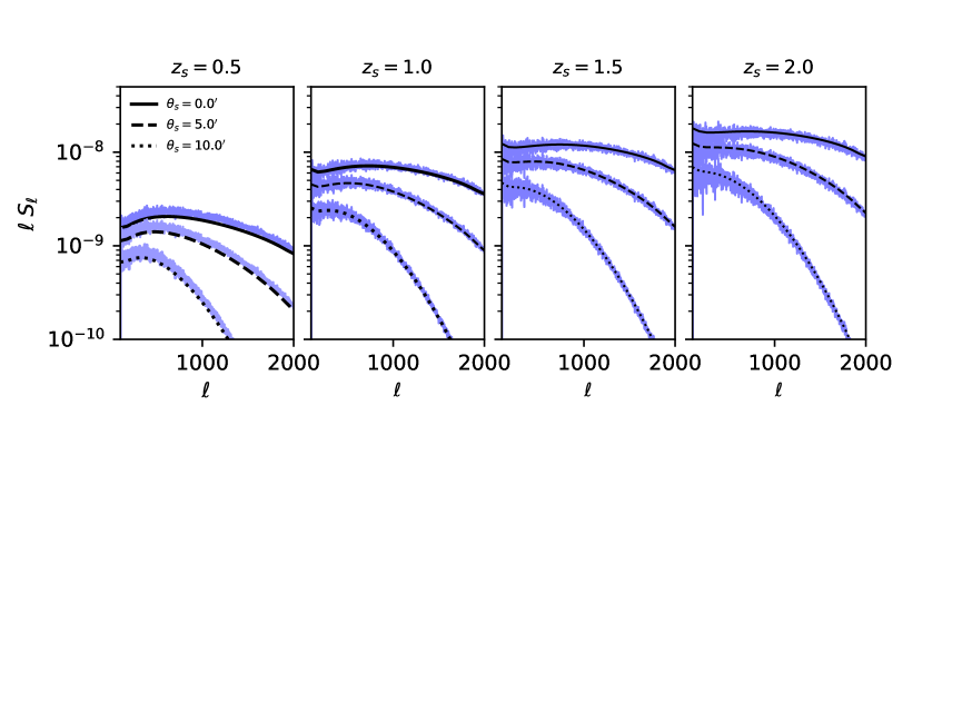
Figure 3: The skew-spectrum $S_{\ell}$ defined in Eq.(25) is being plotted for various smoothing angles and redshifts. The noisy purple lines correspond to results from the simulations. The panels from left to right correspond to redshifts $z_{s}=0.5,1.0,1.5$ and $2.0$. In each panel we show skew-spectra corresponding to Gaussian beams with full width at half maxima of $\theta_{s}=0^{\prime},5^{\prime}$ and $10^{\prime}$, as indicated. We have considered all-sky simulations and no noise was included. The theoretical predictions, shown in black, are computed using the expressions Eq.(17a)-Eq.(17d). The fitting function of (Takahasi et al., 2019) was used throughout this study to model the gravity-induced bispectrum $B_{\delta}$. We use all modes below $\ell_{\rm max}={\rm N}_{\rm side}$ in the computation.

Here, we specialize our discussion to the case of weak lensing surveys. The weak lensing convergence $\kappa$ is a line of sight projection of the 3D density contrast $\delta({\bf r})$ at a comoving distance ${\bm{r}}=(r,{\bm{\theta}})$ using a kernel $w(r)$ defined as follows:

$$\kappa({\bm{\theta}}):=\int_{0}^{r_{s}}drw(r)\delta(r,{\bm{\theta}});\quad w(r):={3\Omega_{\rm M}\over 2}{H_{0}^{2}\over c^{2}}a^{-1}{d_{A}(r)d_{A}({r_{s}-r})\over d_{A}(r_{s})}.$$ (3)

In this expression, $r=|{\bm{r}}|$ is the comoving radial distance to the source, $\bm{\theta}$ describes the angular position on the sky, $\Omega_{M}$ is the cosmological matter density parameter (total matter density in units of the critical density), $H_{0}$ is the Hubble constant, $c$ is the speed of light, $a=1/(1+z)$ is the scale factor at a redshift $z$, $d_{A}(r)$ represents the comoving angular diameter distance at a distance $r$ and $r_{s}$ is the comoving radial distance to the source plane. The corresponding redshift will be represented by $z_{s}$. To keep the analysis simple, in our study we will ignore the source distribution and assume them to be localized on a single source plane defined by $z_{s}$. We will study various statistics as a function of $z_{s}$. To simplify the analysis we will also ignore photometric redshift errors. Needless to say, such complications are essential to link predictions to observational data, and will be presented in an acompanying study.

Fourier decomposing $\delta$ along and perpendicular to the line-of-sight direction we obtain:

$$\kappa(\bm{\theta})=\int_{0}^{r_{s}}dr\omega(r)\int{dk_{\parallel}\over 2\pi}\int{d^{2}{\bf k}_{\perp}\over(2\pi)^{2}}\exp[{\rm i}(rk_{\parallel}+d_{A}(r)\;{\bm{\theta}}\cdot{\bf k}_{\perp})]\delta({\bf k};r).$$ (4)

Here, we have decomposed the 3D wave number ${\bf k}$ along and perpendicular to the radial direction, ${\bf k}=(k_{\parallel},{\bf k}_{\perp})$ We have used the following convention for the 3D Fourier Transform and its inverse:

$$\delta({\bf k})={1\over(2\pi)^{3}}\int d^{3}{\bf r}\exp(-i{\bf k}\cdot{\bf r})\delta({\bf r});\quad\delta({\bf r})=\int d^{3}{\bf k}\exp(i\,{\bf r}\cdot{\bf k})\delta({\bf k}).$$ (5)

The corresponding 3D power spectrum and bispectrum for $\delta$ are:

$$\langle\delta({{\bf k}}_{1})\delta({{\bf k}}_{2})\rangle_{c}:=(2\pi)^{3}\delta_{\rm 3D}({{\bf k}}_{1}+{{\bf k}}_{2})P_{\delta}(k_{1});\quad k=|{\bf k}|;$$ (6)

$$\langle\delta({{\bf k}}_{1})\delta({{\bf k}}_{2})\delta({{\bf k}}_{3})\rangle_{c}:=(3\pi)^{2}\delta_{\rm 3D}({{\bf k}}_{1}+{{\bf k}}_{2}+{{\bf k}}_{3})B_{\delta}({{\bf k}}_{1},{{\bf k}}_{2},{{\bf k}}_{3}).$$ (7)

Using the small-angle approximation the projected power spectrum $P^{\kappa}(l)$ and bispectrum $B^{\kappa}({{\bf{l}}}_{1},{{\bf{l}}}_{2},{{\bf{l}}}_{3})$ of the convergence field $\kappa$ can be expressed respectively in terms of the 3D power spectrum $P_{\delta}(k)$ and bispectrum $B_{\delta}({\bf k}_{1},{\bf k}_{2},{\bf k}_{3})$:

$$P^{\kappa}({l})=\int_{0}^{r_{s}}dr{\omega^{2}(r)\over d_{A}^{2}(r)}P_{\delta}\left({{l}\over d_{A}(r)};r\right);$$ (8a)

$$B^{\kappa}({{\bf{l}}}_{1},{{\bf{l}}}_{2},{{\bf{l}}}_{3})=\int_{0}^{r_{s}}dr{\omega^{3}(r)\over d_{A}^{4}(r)}B_{\delta}\left({{{\bf{l}}}_{1}\over d_{A}(r)},{{{\bf{l}}}_{2}\over d_{A}(r),},{{{\bf{l}}}_{3}\over d_{A}(r)};r\right).$$ (8b)

Detailed derivations of these expressions can be found in (Munshi et al., 2008). Cross-correlating two-tomographic bins can be used to define cross-spectra $P_{\alpha\beta}^{\kappa}$ and cross-skewspectra $B_{\alpha\beta}^{\kappa}$.

$$P_{\alpha\beta}^{\kappa}({l})=\int_{0}^{r_{\rm min}}dr{\omega_{\alpha}(r)\omega_{\beta}(r)\over d_{A}^{2}(r)}P_{\delta}\left({{l}\over d_{A}(r)};r\right);$$ (9a)

$$B_{\alpha\beta}^{\kappa}({{\bf{l}}}_{1},{{\bf{l}}}_{2},{{\bf{l}}}_{3})=\int_{0}^{r_{\rm min}}dr{\omega_{\alpha}^{1}(r)\omega_{\beta}^{2}(r)\over d_{A}^{4}(r)}B_{\delta}\left({{{\bf{l}}}_{1}\over d_{A}(r)},{{{\bf{l}}}_{2}\over d_{A}(r),},{{{\bf{l}}}_{3}\over d_{A}(r)};r\right);\quad r_{min}=min(r_{\alpha},r_{\beta});$$ (9b)

$$w_{i}(r):={3\Omega_{\rm M}\over 2}{H_{0}^{2}\over c^{2}}a^{-1}{d_{A}(r)d_{A}({r_{si}-r})\over d_{A}(r_{si})};\quad i\in\{\alpha,\beta\}.$$ (9c)

The integration takes contribution only from the overlapping redshift range of the two bins. Thus, the upper-limit extends only to the source plane defined by the lower redshift $r_{\rm min}={\rm min}(r_{\alpha},r_{\beta})$. Notice that $P^{\kappa}_{\alpha\beta}=P^{\kappa}_{\beta\alpha}$ but $B^{\kappa}_{\alpha\beta}\neq B^{\kappa}_{\beta\alpha}$ and they carry independent information. It is possible to directly deal with shear bispectrum and relate them to density bispectrum thus avoiding the map making process. See (Munshi et al., 2011d) for bispectra constructed for higher-spin objects, i.e. shear as well as flexions.

3.2 Skew-spectrum in all-sky and flat-sky

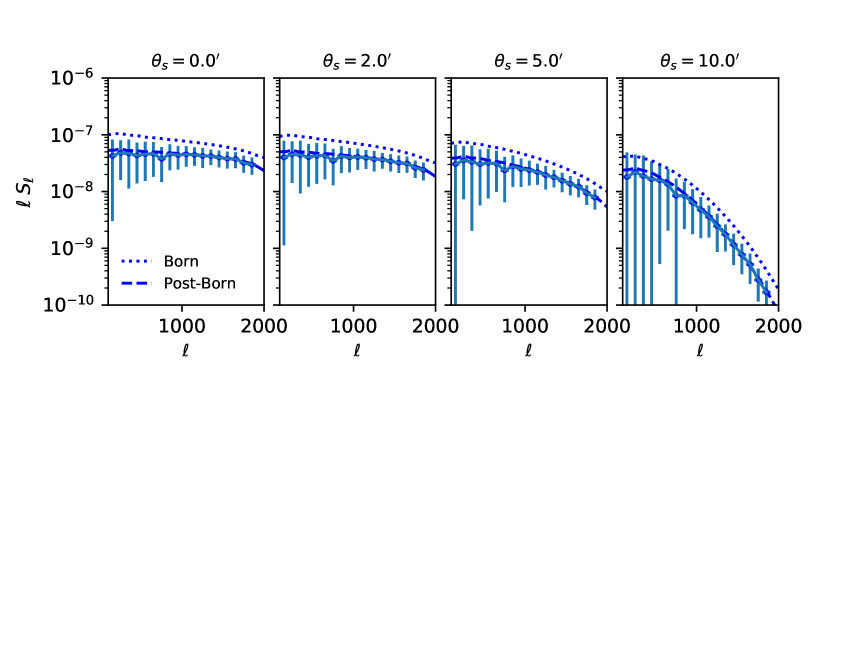
Figure 4: The skew-spectra $S_{\ell}$ defined in Eq.(25) for the CMB is being plotted for various smoothing angles. The smooth dashed and dotted lines correspond to theoretical predictins. The points with error-bars correspond to measurements from numerical simulations. The panels from left to right correspond to various smoothing beams of Full Width at Half Maximum (FWHM) $\theta_{s}=0.^{\prime},2.0^{\prime},5.0^{\prime}$ and $10^{\prime}$. respectively. We have considered all-sky simulations and no noise was included. The theoretical predictions are computed using (Takahasi et al., 2019). The dotted curves in each panels are computed using the Born approximation, whereas the dashed curves are computed using more accurate post-Born approximation. The error-bars are computed using ten different realisations of the simulations. The plots underline the importance of post-Born correction in the computation skew-spectrum. Although such corrections can safely be ignored at lower redshifts.

The skew-spectrum statistic for $\kappa$ is constructed by cross-correlating the squared $\kappa$ with itself. We start by introducing the spherical harmonic transform of a convergence map $\kappa({\hat{\Omega}})$ defined over the surface of the sky using spherical harmonics $Y_{\ell m}({\hat{\Omega}})$ to define the multipoles $\kappa_{\ell m}$:

$$\kappa_{\ell m}:=\int\,d{{\hat{\Omega}}}\,Y_{\ell m}\,\kappa({{\hat{\Omega}}});\quad{\hat{\Omega}}=(\vartheta,\varphi);\;\;d{\hat{\Omega}}=\sin\vartheta\,d\vartheta\,d\varphi.$$ (10)

Any Gaussian field is completely characterized by its power spectrum ${\cal C}^{\kappa}_{\ell}$ which is defined as ${\cal C}^{\kappa}_{\ell}:=\langle\kappa_{\ell m}\kappa^{*}_{\ell m}\rangle$. In the flat-sky limit the power spectrum $P^{\kappa}(l)$ is identical to ${\cal C}^{\kappa}_{\ell}$ at high $\ell$ with the identification $l=\ell$. The weak lensing $\kappa$ maps are highly non-Gaussian. The bispectrum is the lowest-order statistics that characterizes departure from Gaussianity is defined as the three-point coupling of harmonic coefficients. The statistics beyond bispectra, e.g., the trispectra and its higher-order analogs are increasingly noise dominated. By assuming isotropy and homogeneity the all-sky bispectrum $B^{\kappa}_{\ell_{1}\ell_{2}\ell_{3}}$ is defined as:

$$\langle\kappa_{\ell_{1}m_{1}}\kappa_{\ell_{2}m_{2}}\kappa_{\ell_{3}m_{3}}\rangle_{c}\equiv B^{\kappa}_{\ell_{1}\ell_{2}\ell_{3}}\left(\begin{array}[]{ c c c }\ell_{1}&\ell_{2}&\ell_{3}\\ 0&0&0\end{array}\right).$$ (13)

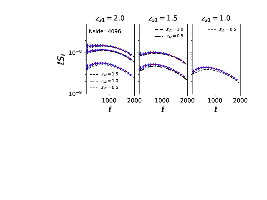
Figure 5: The skew-spectra computed by cross-correlating $\kappa^{2}$ and $\kappa$ from two different redshift bins is plotted. In particular, the squared $\kappa_{1}=\kappa(z_{s1})$ defined for a source redshift $z_{s1}$ and $\kappa_{s2}=\kappa(z_{s2})$ at redshift $z_{s2}$ are being cross-correlated in the harmonic domain. For this plot we restricted ourselves to $z_{s1}>z_{s2}$. The smooth lines correspond to the theoretical predictions and the lines with error bars correspond to results from numerical simulations. We use the expression of mixed bispectrum given in Eq.(9b)-Eq.(9c) for computing the theoretical predictions. The expression for the estimator for the skew-spectrum is given in Eq.(25). The panels from left to right correspond to $z_{s1}=2.0,1.5$ and $1.0$ respectively and various curves in each panel correspond to $z_{2}$ as indicated. The maps used were constructed at Healpix resolution $N_{\rm side}=4096$. We have filtered all $\ell>2048$ modes out before analysing them. No additional smoothing was considered. We do not include any noise due to intrinsic ellipticity distribution of galaxies. We have used one single all-sky realisation to compute the skew-spectra and no mask was included.

Here the quantity in parentheses is the well-known Wigner-$3j$ symbol which enforces the rotational invariance. It is only non-zero for the triplets $(\ell_{1},\ell_{2},\ell_{3})$ that satisfy the trinagular condition and $\ell_{1}+\ell_{2}+\ell_{3}$ is even. The reduced bispectrum $b^{\kappa}_{\ell_{1}\ell_{2}\ell_{3}}$ is useful in directly linking the all-sky bispectrum and its flat-sky counterpart. For the convergence field $\kappa$, $b^{\kappa}_{\ell_{1}\ell_{2}\ell_{3}}$ is defined through the following expression:

$$B^{\kappa}_{\ell_{1}\ell_{2}\ell_{3}}:=\sqrt{(2\ell_{1}+1)(2\ell_{2}+1)(2\ell_{3}+1)\over 4\pi}\left(\begin{array}[]{ c c c }\ell_{1}&\ell_{2}&\ell_{3}\\ 0&0&0\end{array}\right)b^{\kappa}_{\ell_{1}\ell_{2}\ell_{3}}.$$ (16)

Finally we are in a position to define the skew spectrum as the cross power-spectra formed by cross-correlating the squared $\kappa^{2}({\hat{\Omega}})$ maps against the original map $\kappa({\hat{\Omega}})$.

$${\cal S}_{\ell}:={1\over 2\ell+1}\sum_{m}{\rm Real}\{[\kappa^{2}]_{\ell m}[\kappa]^{*}_{\ell m}\}=\sum_{\ell_{1}\ell_{2}}B^{\kappa}_{\ell_{1}\ell_{2}\ell}J_{\ell_{1}\ell_{2}\ell};$$ (17a)

$$J_{\ell_{1}\ell_{2}\ell}:=\sqrt{{(2\ell_{1}+1)(2\ell_{2}+1)\over 4\pi(2\ell+1)}}\left(\begin{array}[]{ c c c }\ell_{1}&\ell_{2}&\ell\\ 0&0&0\end{array}\right).$$ (17d)

Here $[\kappa^{2}]_{\ell m}$ represents the harmonic multipoles computed using a harmonic decomposition of $\kappa^{2}$ and ^∗ denotes complex conjugation. The commonly used (normalised) one-point skewness parameter $S_{3}={\langle\kappa^{3}\rangle_{c}/\langle\kappa^{2}\rangle_{c}^{2}}$ can be recovered from the skew-spectrum. The third-order moment $\langle\kappa^{3}\rangle$ is given by:

$$\langle\kappa^{3}(\theta_{s})\rangle_{c}={1\over 4\pi}\sum_{\ell}(2\ell+1)S_{\ell}{\beta}^{3}_{\ell}(\theta_{s});$$ (18)

The smoothing beam (window) is denoted as ${\beta}_{\ell}(\theta_{s})$. Being a two-point statistic, the skew-spectrum $S_{\ell}$ is related to the two-to-one correlation function $\xi^{21}$ in the real space. They are related by the following expression:

$$\xi^{21}(\theta_{12}):=\langle\kappa^{2}(\theta_{1})\kappa(\theta_{2})\rangle_{c}={1\over 4\pi}\sum_{\ell}(2\ell+1)S_{\ell}P_{\ell}(\cos\theta_{12}){\beta}^{3}_{\ell}(\theta_{s}).$$ (19)

Here $P_{\ell}$ is the Legendre Polynomial and $\beta_{\ell}$ is the Gaussian smoothing beam with Full Width at Half Maximum (FWHM) of $\theta_{s}$. Suitably normalised two-to-one correlators is the lowest order of a family of statistics also known as cumulant correlator (Bernardeau, 1996), it has also been used in the context of weak-lensing surveys (Munshi, 2000). The flat-sky bispectrum is similarly defined through:

$$\langle\kappa({\bf{l}}_{1})\kappa({\bf{l}}_{2})\kappa({\bf{l}}_{3})\rangle_{c}=(2\pi)^{2}\delta_{2D}({\bf{l}}_{1}+{\bf{l}}_{2}+{\bf{l}}_{3})B^{\kappa}({\bf{l}}_{1},{\bf{l}}_{2},{\bf{l}}_{3}).$$ (20)

The flat-sky bispectrum $B^{\kappa}({\bf{l}}_{1},{\bf{l}}_{2},{\bf{l}}_{3})$ is identical to the reduced bispectrum $b_{\ell_{1}\ell_{2}\ell_{2}}$ for high multipole (Bartolo et al., 2004). This can be shown by using the following asymptotic relationship:

$${\cal G}_{\ell_{1}m_{1},\ell_{2}m_{2},\ell_{3}m_{3}}\equiv\int d{\hat{\Omega}}Y_{\ell_{1}m_{1}}({\hat{\Omega}})Y_{\ell_{2}m_{2}}({\hat{\Omega}})Y_{\ell_{3}m_{3}}({\hat{\Omega}}){}$$

$$=\sqrt{{(2\ell_{1}+1)(2\ell_{2}+1)(2\ell+1)\over 4\pi}}\left(\begin{array}[]{ c c c }\ell_{1}&\ell_{2}&\ell\\ 0&0&0\end{array}\right)\left(\begin{array}[]{ c c c }\ell_{1}&\ell_{2}&\ell\\ m_{1}&m_{2}&m_{3}\end{array}\right)\approx(2\pi)^{2}\delta_{\rm 2D}({\bf{l}}_{1}+{\bf{l}}_{2}+{\bf{l}}_{3}).$$ (21e)

The skew-spectrum in the flat-sky is given by (Pratten & Munshi, 2012):

$$\mathcal{S}(l_{2})=\int_{0}^{\infty}{l_{1}dl_{1}\over 2\pi}\int^{1}_{-1}{d\mu\over 2\pi\sqrt{1-\mu^{2}}}B^{\kappa}({\bf{l}}_{1},{\bf{l}}_{2},-({\bf{l}}_{1}+{\bf{l}}_{2}))\beta(l_{1}\theta_{s})\beta(l_{2}\theta_{s})\beta(|{\bf{l}}_{1}+{\bf{l}}_{2}|\theta_{s}).$$ (22)

In our notation $\mu=({{\bf{l}}_{1}\cdot{\bf{l}}_{2}/l_{1}l_{2}})$, and we have used $\beta_{\ell_{1}}(\theta_{s})=\beta(l_{1}\theta_{s})$ to denote the flat-sky beam. In the high-$l$ limit we have $\mathcal{S}(l_{2})\rightarrow S_{\ell_{2}}$.

Here a few comments about the skew-spectrum are in order. The one-point statistics such as the skewness parameter has the advantage of having high signal-to-noise. However, it lacks distinguishing power as all the available information in the bispectrum is compressed into a single number. Therefore, such statistics can not distinguish various contributions, e.g. from primordial non-Gaussianity or non-Gaussianity from intrinsic alignment of source galaxies from the gravity induced secondary non-Gaussianity. The skew-spectrum, on the other hand, retains some of the information regarding the shape of the spectrum, thus it can in principle allow to separate various contributions or remove possible source of contamination from systematics.

In this paper we have considered a direct estimator for the skew-spectrum as opposed to the optimal estimator developed in (Komatsu, Spergel, Wandelt, 2005; Munshi & Heavens, 2010) where optimality was achieved by using suitable weights to the harmonics that incorporates a match filtering as well as saturates the Cramer-Rao limit in the weakly non-Gaussian limit. Indeed, a simple Fisher matrix based analysis will no longer be adequate for moderately non-Gaussian weak lensing maps. However optimality is not of crucial importance for analysing weak lensing maps as the secondary non-Gaussianity is expected to detected with much higher signal-to-noise. A direct estimator which is simpler to implement will thus be useful for studying non-Gaussianity in weak-lensing maps.

Next we consider skew-spectrum for specific models of bispectrum considered in §2.

3.3 The skew-spectrum in the tree-level Standard Perturbation Theory (SPT)

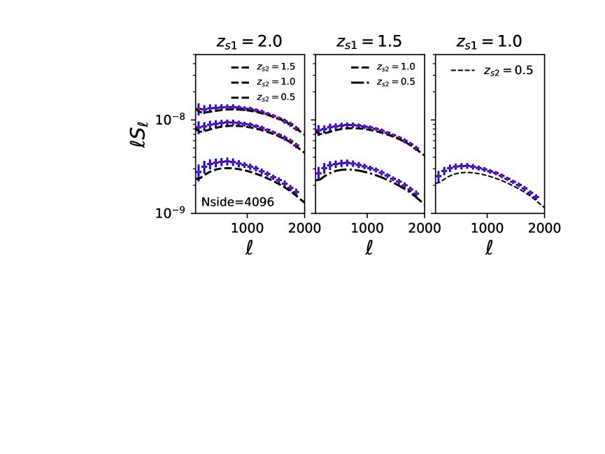
Figure 6: Same as Figure-5 but the skew-spectrum is being computed cross-correlating $\kappa_{1}$ and $\kappa_{2}^{2}$ instead of $\kappa_{1}^{2}$ and $\kappa_{2}$ for $z_{s1}>z_{s2}$.

Analytical predictions for the skew-spectrum for large smoothing angular scales can be obtained using perturbative calculations. The low $\ell$ limit of the skew-spectrum and its higher-order generalisations were recently presented in (Munshi & McEwen, 2020). This is possible using a technique based on a generating function formalism. However, for arbitrary $\ell$ an order-by-order calculation is needed. We will obtain these results using a Gaussian smoothing beam where complete analytical results in closed form can be derived. We will consider the gravity induced (secondary) non-Gaussianity.

$$S(l_{2})=\int dr\;{w^{3}(r)\over d_{A}^{4}(r)}\int\frac{l_{1}dl_{1}}{(2\pi)^{2}}P_{\delta}\left({l_{1}\over d_{a}(r)};r\right)P_{\delta}\left({l_{2}\over d_{a}(r)};r\right)\beta^{2}(l_{1}\theta_{s})\beta^{2}(l_{2}\theta_{s}){\cal T}(l_{1}l_{2})$$ (23a)

$${\cal T}(l_{1}l_{2})=\Bigg{[}\frac{36}{7}I_{0}(l_{1}l_{2}\theta_{s}^{2})-3\left(\frac{l_{1}}{l_{2}}+\frac{l_{2}}{l_{1}}\right)I_{1}(l_{1}l_{2}\theta_{s}^{2})+\frac{6}{7}I_{2}(l_{1}l_{2}\theta_{s}^{2})\Bigg{]}.$$ (23b)

The angular integral in Eq.(22) can be done analytically using the Modified Bessel Functions represented in $I_{m}$. To simplify the notation we adopt a parameterisation in terms of the variables $C^{\alpha\beta}_{m}$:

$$S(l_{2})=\,\sigma_{L}^{2}P^{\kappa}(l_{2})R_{2}\int\frac{l_{1}dl_{1}}{2\pi}l_{1}^{n}l_{2}^{n}\beta^{2}(l_{1}\theta_{s})\beta^{2}(l_{2}\theta_{s}){\cal T}(l_{1}l_{2});$$ (24a)

$$R_{2}=\int_{0}^{r_{s}}dr{w^{3}(r)\over d^{4+2n}_{A}(r)}D^{4}_{+}(z)/\left[\int_{0}^{r_{s}}dr{w^{2}(r)\over d^{2+n}_{A}(r)}D^{2}_{+}(z)\right]^{2}.$$ (24b)

To separate the temporal $r$ and angular $l$ parts of the integral we replaced the linear power spectrum $P_{\delta}(k)$ with a power-law form, i.e. $P_{\delta}(k)=AD^{2}_{+}(z)k^{n}$. Due to the choice of normalisation here the skew-spectrum is independent of the power spectrum amplitude $A$. The resulting skewness $S_{3}$ can then be written as:

$$S_{3}:={\int l_{2}\,d\,l_{2}\,}S(l_{2})\,\quad\quad$$ (25)

The $F_{2}$ kernel for many modified gravity theories have a similar structural form and can be treated analytically. Similarly, the Effective Field Theory based approaches introduces corrective terms to $F_{2}$ that too have a very similar form (Munshi & Regan, 2012). The kernel describing the primordial non-Gaussianity can also be treated in a similar manner. We will focus on certain well known cases of modified gravity theories. The analytical results for these models are important as there are no established numerical fitting-function available in these scenarios.

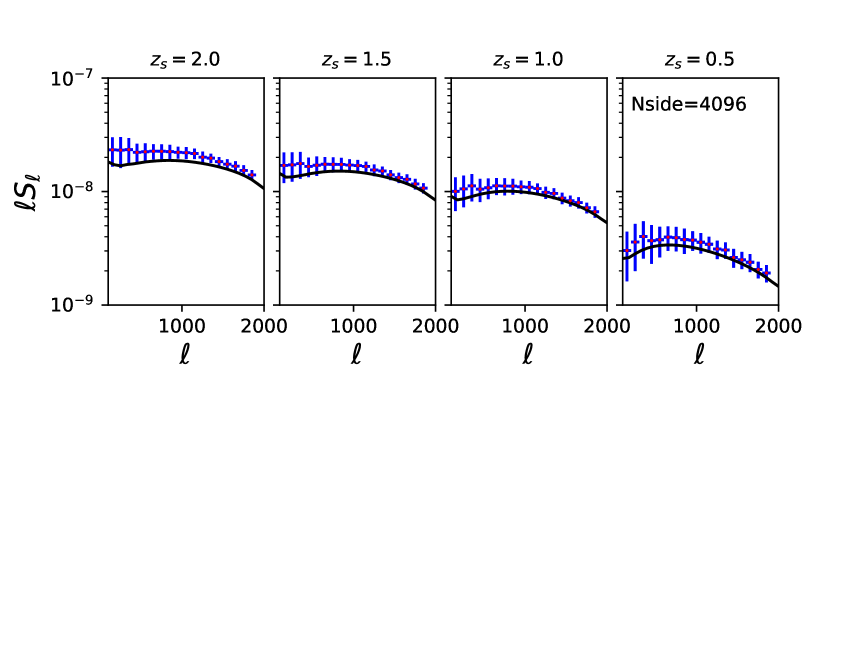
Figure 7: The skew-spectra computed by cross-correlating $\kappa^{2}_{\rm LSS}$ at the last scattering surface of $z_{LSS}=1100$ and low redshift weak lensing convergence maps at $z_{s}$ is being plotted. As before the solid smooth lines in different panels correspond to theoretical results and the lines with error bars correspond to the results from numerical simulations. The panels from left to right correspond to $z_{s}=2.0,1.5,1.0$ and $0.5$ respectively. No mask or smoothing was considered. We use the expression of mixed bispectrum given in Eq.(9b)-Eq.(9c) for computing the theoretical predictions.

4 Numerical Simulations

We use the publicly available all-sky weak lensing maps generated by (Takahashi et al., 2017) that were generated using ray-tracing through N-body simulations. The underlying simulations followed the gravitational clustering of $2048^{3}$ particles. Multiple lens planes were used to generate convergence $\kappa$ and the corresponding shear $\gamma$ maps. To generate the maps in these simulations, the source redshifts used were in the range $z_{s}=0.05-5.30$ at an interval $\Delta z_{s}=0.05$. In our study, we have used the maps with $z_{s}=0.5,1.0,1.5,2.0$. For CMB maps the lensing potentials were constructed using the deflection angles which were used to construct the lensing potentials and eventually the $\kappa$ maps. In recent studies inclusion of post-Born terms in lensing statistics were outlined (Pratten & Lewis, 2016). The maps we use include post-Born corrections. In this study we will see that at the low source redshift such corrections play a negligible role although they play a significant role at higher redshift, e.g. in case of lensing of CMB. The convergence maps were generated using an equal area pixelisation scheme in HEALPix format(Gorski et al., 2016). In this pixelisation scheme the number of pixels scale as $N_{\rm pix}=12N^{2}_{\rm side}$ where $N_{\rm side}$ is the resolution parameter which can take values $N_{\rm side}=2^{N}$ with $N=1,2,\cdots$. The set of maps we use in this study are generated at $N_{\rm side}=4096$ and were cross-checked against higher resolution maps constructed at a resolution $N_{\rm side}=8192,16384$ for consistency. These maps constructed at different resolution were found to be consistent with each other up to the angular harmonics $\ell\leq 2000$. Various additional tests were also performed using an Electric/Magnetic (E/B) decomposition of the shear maps for the construction of $\kappa$ maps (Takahashi et al., 2017). We have used high resolution maps $N_{\rm side}=4096$. We have degraded these maps to $N_{\rm side}=2048$ and analysed them for harmonic modes satisfying $\ell<2N_{\rm side}$. The background cosmological parameters used for these simulations are: $\Omega_{\rm CDM}=0.233$, $\Omega_{b}=0.046$, $\Omega_{\rm M}=\Omega_{\rm CDM}+\Omega_{b},\Omega_{\Lambda}=1-\Omega_{\rm M}$ and $h=0.7$. The amplitude of density fluctuation $\sigma_{8}=0.82$ and the spectral index $n_{s}=0.97$. Examples of $\kappa$ maps used in our study are presented in Figure-1. It is also worth mentioning that these maps were also used to recently analyze the bispectrum the context of CMB lensing (Namikawa et al., 2018) and for weak lensing of galaxies at low redhifts (Munshi et al., 2019a; Munshi & McEwen, 2020).

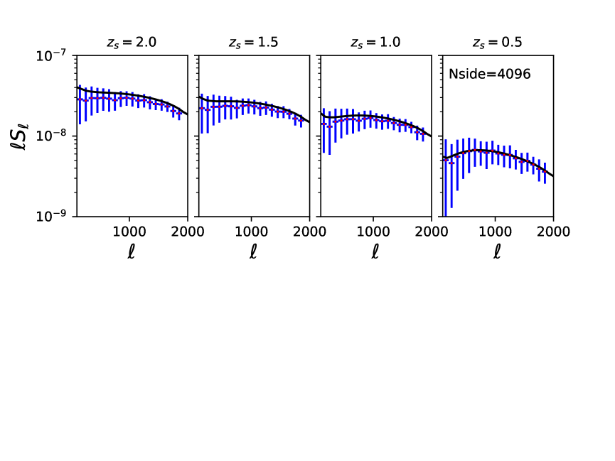
Figure 8: Same as Figure-7 but are constructed by cross-correlating $\kappa_{\rm LSS}$ against $\kappa^{2}_{s}$.

5 The Pseudo Skew-Spectrum Estimator

The optimal Maximum Likelihood (ML) estimators or the quadratic maximum likelihood (QML) estimators (Efsthathiou, 2004) are often used for analyzing cosmological data sets. The optimality of these estimators require inverse covariance weighting of the input data vector which clearly is not practical for large cosmological data sets though various clever algorithmic techniques have been considered (Oh, Spergel, Hinshaw, 1990). As a result many sub-optimal estimators, which use heuristic weighting schemes, have been developed. The so-called pseudo-$\cal C_{\ell}$ (PCL) technique was introduced in (Hivon et al., 2002) in the harmonic domain. Later a related correlation function based approach was introduced in Szapudi et al. (2001). These estimators are unbiased but are sub-optimal. Typically various heuristic weighting depending on sky coverage, as well as noise characteristics can improve the optimality of these estimators typically in noise dominated high-$\ell$ (or smaller angular scales) regime. The maximum likelihood estimators on the other hand can be efficiently used for larger smoothing scales. Different hybridization schemes can be used to combine the large angular scale (equivalently the low $\ell$) estimates using QML with small angular scale (high $\ell$) PCL estimates (Efsthathiou, 2004). In our study we will use a direct pseudo-$\cal C_{\ell}$ estimator for the skew-spectrum. The direct estimator from the masked sky ${\tilde{S}}_{\ell}$ is related to the underlying all-sky $S_{\ell}$ skew-spectrum through a mode-mixing matrix $M_{\ell\ell^{\prime}}$ that depends on the mask.

$${\tilde{S}}_{\ell}=M_{\ell\ell^{\prime}}S_{\ell};\quad{\hat{S}}_{\ell}=M^{-1}_{\ell\ell^{\prime}}{\tilde{S}}_{\ell};\quad\langle{\hat{S}}_{\ell}\rangle=S_{\ell}.$$ (26a)

Here $\tilde{\cal S}_{\ell^{\prime}}^{(21)}$ denotes the skew-spectrum computed from a map in the presence of a mask $w({\hat{\Omega}})$, $\hat{\cal S}_{\ell^{\prime}}^{(21)}$ is the all-sky estimate. The mode-coupling matrix $M_{\ell\ell^{\prime}}$ is given in terms of the power spectrum of the mask $w({\hat{\Omega}})$ as follows:

$$M_{\ell\ell^{\prime}}=(2\ell^{\prime}+1)\sum_{\ell^{\prime\prime}}\left(\begin{array}[]{ c c c }\ell&\ell^{\prime}&\ell^{\prime\prime}\\ 0&0&0\end{array}\right)^{2}{(2\ell^{\prime\prime}+1)\over 4\pi}|w_{\ell^{\prime\prime}}^{2}|;$$ (29)

Here $w_{\ell}={1/(2\ell+1)}\sum_{m}w_{\ell m}w^{*}_{\ell m}$ is the power spectrum of the mask constructed from the harmonic-coefficient $w_{\ell m}$ of the map. The coupling matrix $M_{\ell\ell^{\prime}}$ encodes the mode-mixing due to the presence of a mask. We have used this estimator for estimation of skew-spectrum from individual tomographic bins as well as cross-correlating two different bins. In case of cross-correlation we have used the same mask for the two different bins. The generalization of the PCL method to estimate higher-order spectra were developed in (Munshi et al., 2011a, b) for spin-0 fields and in higher spin fields in (Munshi et al., 2011d) as well as in 3D in (Munshi et al., 2011e).

In our study, we have used the mask which is shown in Figure-2. To construct this mask all pixels (shown in maroon) lying within $22$ degree of either the galactic or ecliptic planes are discarded. The remaining unmasked pixels cover $14,490$ degree² of the sky, making fraction of the sky covered $f_{\rm sky}\approx 0.35$ (Taylor et al., 2019). Various aspects of noise involved in cross-correlating CMB lensing maps and galaxy lensing maps are discussed in (Fabbian, Lewis, Beck, 2019).

Typically, to construct an unbiased PCL estimator the noise contribution is subtracted from the total estimates. This however is not necessary for the construction of the skew-spectrum estimator as the bispectrum of a Gaussian noise is zero. However, presence of noise in the data does increase the variance of the estimator. We will not attempt to construct the covariance matrix of our estimator. Such a generalization will be presented in a future publication.

6 Results and Discussion

In this section we discuss the numerical results presented in this paper. We have used all-sky simulations generated at $N_{\rm side}=4096$ for validating the theoretical predictions. We have used the simulations generated at lower redshifts for weak lensing studies along with the lensing maps generated at $z_{s}=1100$ (last scattering surface). Examples of the maps used in our study are presented in Figure-1. The mask used in studying the effect of mask on estimation of skew-spectrum is presented in Figure-2. We have used these maps for constructing the skew-spectra at individual redshift as well as computing the skew-spectrum by cross-correlating two different redshifts. Below we list our findings.

Figure 9: The pseudo-${\cal S}_{\ell}$ for two different redshifts are presented. A Euclid type mask was used in our study. The regions which are within $22\,\rm deg$  of the galactic or ecliptic plane are removed from our study. The fraction of the sky left unmasked is $f_{\rm sky}=0.35\;$ (roughly $14,490$ deg² of the sky). The left (right) panel corresponds to $z_{s}=1.0(z_{s}=2.0)$. The upper smooth solid curves represents the theoretical $S_{\ell}$. The two upper curves represent estimated skew-spectrum from a single realisation. The curve that shows more scatter represents skew-spectrum estimated from an all-sky map. The curve whcih shows more scatter correspond to ${\hat{S}}_{\ell}$ using Eq.(26a) and Eq.(26a).

Figure 10: The impact of noise (assumed Gaussian) on estimation of skew-spectrum is presented. In both panels the source plane is fixed at $z_{s}$=1. The solid lines in each panel represent the theoretical skew-spectrum for $z_{s}=1$. The dashed line represent the pseudo skew-spectrum or $\tilde{S}_{l}$ for the Euclid-type mask being considered. Inclusion of Gaussian noise increases the scatter but the estimator remains unbiased. The left-panel corresponds to source density of $n_{s}=30\;{\rm arcmin}^{-2}$ and the right-panel corresponds to $n_{s}=10\;{\rm arcmin}^{-2}$.

1. Skew-spectra from Individual Tomographic Bins: First, we compute the theoretical skew-spectra $S_{\ell}$ using Eq.(25) as a function of harmonics $\ell$ for various smoothing angular scales as well as redshifts. The results for lower redshift bins are plotted in Figure -3 and the results for the last scattering surface (LSS) is plotted in Figure -4. In Figure -3 the panels from left to right correspond to redshifts $z_{s}=0.5,1.0,1.5$ and $2.0$. In each panel three different smoothing angular scales are considered, from top to bottom the curves correspond to full width half maxima (FWHM) of the Gaussian beam $\theta_{s}=0.0^{\prime},5.0^{\prime}$ and $10^{\prime}$ as indicated. For the CMB sky shown in Figure -4 the panels from left to right correspond to four different Gaussian beams $\theta_{s}=0.0^{\prime},5.0^{\prime}$ and $10^{\prime}$. We have computed the skew-spectra using the Born-approximation as well as including the post Born correction terms (Pratten & Lewis, 2016). We found that the post-Born corrections will be important in modelling the skew-spectra at high redshifts. However, for the lower redshifts we found this corrections to be negligible as expected. We have considered all-sky simulations and no noise was included. The theoretical predictions are computed using the expressions Eq.(17a)-Eq.(17d). The fitting function of (Takahasi et al., 2019) was used throughout in this study to model the gravity-induced bispectrum $B_{\delta}$. We use all modes below $\ell_{max}=2{\rm N}_{\rm side}$ in our computation. We have also removed all modes $\ell_{max}<100$ from our computation. These fitting-functions are found to be an excellent description of the simulated data.

2. Cross-correlating Two Tomographic Bins: The skew-spectra computed by cross-correlating $\kappa^{2}({\hat{\Omega}})$ and $\kappa({\hat{\Omega}})$ from two different redshift bins is being plotted in Figure-5 and Figure-6. In particular, squared $\kappa_{1}=\kappa(z_{1})$ defined for a source redshift $z_{1}$ and $\kappa_{2}=\kappa(z_{2})$ at redshift $z_{2}$ is being cross-correlated in the harmonic domain. For this plot we restrict ourselves to $z_{1}>z_{2}$. We use the expression of mixed bispectrum given in Eq.(9b)-Eq.(9c) for computing the theoretical predictions. The expression for the estimator for the skew-spectrum is given in Eq.(25). From left to right panels correspond to $z_{1}=2.0,1.5$ and $1.0$ respectively and various curves in each panel correspond to $z_{2}$ as indicated. The maps used were constructed at Healpix resolution $N_{\rm side}=4096$. We have filtered all $\ell>2048$ modes out before analyzing them. No additional smoothing was considered. We do not include any noise due to intrinsic ellipticity distribution of galaxies. We have used one single all-sky realization to compute the skew-spectra and no mask was included. The skew-spectra constructed by cross-correlating $\kappa^{2}$ at the Last Scattering Surface (LSS, $z_{s}=1100$) and $\kappa$ at lower redshift is presented in Figure-7. Similarly, the skew-spectrum constructed using $\kappa$ at LSS and $\kappa^{2}$ at lower redshift is presented in Figure-8. We found that the post-Born correction is negligible in modelling the skew-spectrum constructed cross-correlating maps from two redshifts.

3. Accuracy of Predictions: To quantify the difference of predicted skew-spectra and the one estimated from numerical simulation we have used the following statistics:

   $$\Delta_{b}={1\over\sigma_{b}}\left[\hat{S_{b}}-S^{th}_{b}\right].$$ (30)

   Here $\hat{S}_{b}$ represents the binned theoretical skew-spectrum and $S^{th}_{b}$ is the estimated binned skew-spectrum from numerical simulation and $\sigma_{b}$ is the standard deviation of the fluctuations in individual $\ell$ modes within a bin. We have chosen a bin-size of $\delta_{b}$. The results are shown in Figure-11. The left panel shows the errors in skew-spectra obtained by cross-correlating $\kappa^{2}_{\rm LSS}$ and low redshift $\kappa$ (upper curves) and their symmetric counterparts (lower curves). The fitting functions under-predict the simulation results for $\langle\kappa^{2}_{\rm LSS}\kappa\rangle$ and under-predicts the results for skew-spectra associated with $\langle\kappa_{\rm LSS}\kappa^{2}\rangle$. The difference between theory and simulation is lowest for $z_{s}=0.5$ and increases with the redshift. For $z_{s}=2.0$ it can be as high as $1.5\sigma_{b}$. The results are more pronounced for the intermediate bins. The middle- and right panels of Figure-11 depicts $\Delta_{b}$ for $\kappa_{1}^{2}\kappa_{2}$ (middle-panel) and $\kappa_{2}^{2}\kappa_{1}$ respectively. The difference is highest for skew-spectra involving $z_{s}=0.5$ and lower for higher redshift $z_{s}=2.0$. The $\Delta_{b}$ can reach a value of $2.5$ for lower redshifts. The theory typically under-predicts the data.

   The individual skew-spectral bins are correlated as the skew-spectrum is an integrated measure, i.e., individual $\ell$ modes (bins) depend on the entire range of $\ell$ modes (bins). So a straight forward $\chi^{2}$ analysis (using a diagonal covariance matrix) is not possible. Nevertheless, notice that we have considered noise-free simulations in charachterization of errors. Inclusions of noise will increase $\sigma_{b}$ and decrease $\Delta_{b}$. We have considered full-sky maps but, inclusion of the masks will increase the scatter and thus further reduce the value of $\Delta_{b}$. Hence, the deviations seen here should be seen as a maximum possible deviation for the chosen ${\rm N}_{\rm side}$.

4. Mask: We have examined the impact of an Euclid type mask on skew-spectrum in a Pseudo-${\cal C}_{\ell}$ based approach introduced in §5. The results are presented in Figure - 9. The upper solid-lines in each panel correspond to to all-sky theoretical predictions of $S_{\ell}$. The upper lines with scatter correspond to the estimates from one relaisation of the simulated maps. The left-panel corresponds to the source redshift $z_{s}=1.0$ and the right-panel corresponds to $z_{s}=2.0$. The lower dashed-curves in each panel correspond to the PCL based theoretical predictions $\tilde{S}_{\ell}$ computed using Eq.(26a). The corresponding (lower) lines with scatter are estimates from one realisation of partial sky with the Euclid-type mask, shown in Figure-2, applied.

5. Noise: The impact of noise which we assume to be Gaussian on estimation of skew-spectrum is shown in Figure - 10. In both panels the source plane is fixed at $z_{s}$=1. The solid lines in each panel represent the theoretical skew-spectrum for $z_{s}=1$. The dashed lines represent the pseudo skew-spectrum represented as $\tilde{S}_{l}$ with an Euclid-type mask being included. If we compare the scatter with corresponding plots in Figure-9 we can see how the inclusion of noise increases the scatter though the estimator remains unbiased. skew-spectrum for a Gaussian noise alone is zero so the only effect the noise has on the estimator is to increase its scatter.

   The noise was generated at each pixel using a Gaussian deviate with variance $\sigma={\sigma_{\epsilon}/\sqrt{\bar{n}}}$. Where we take $\sigma_{\epsilon}$ represents the variance of the observed ellipticity $\sigma_{\epsilon}=0.3$, and $\bar{n}$ is the average number density of source galaxies per pixel computed using total number of observed galaxies, fraction of sky covered and number of pixel at a specific healpix resolution. We have used two different values of $\bar{n}$. The left-panel of Figure-10 corresponds to a source density of $n_{s}=30\;{\rm arcmin}^{-2}$ and the right-panel corresponds to $n_{s}=10\;{\rm arcmin}^{-2}$. The fraction of the sky covered by the mask was taken to be $f_{\rm sky}=0.35$.

7 Conclusions and Future Prospects

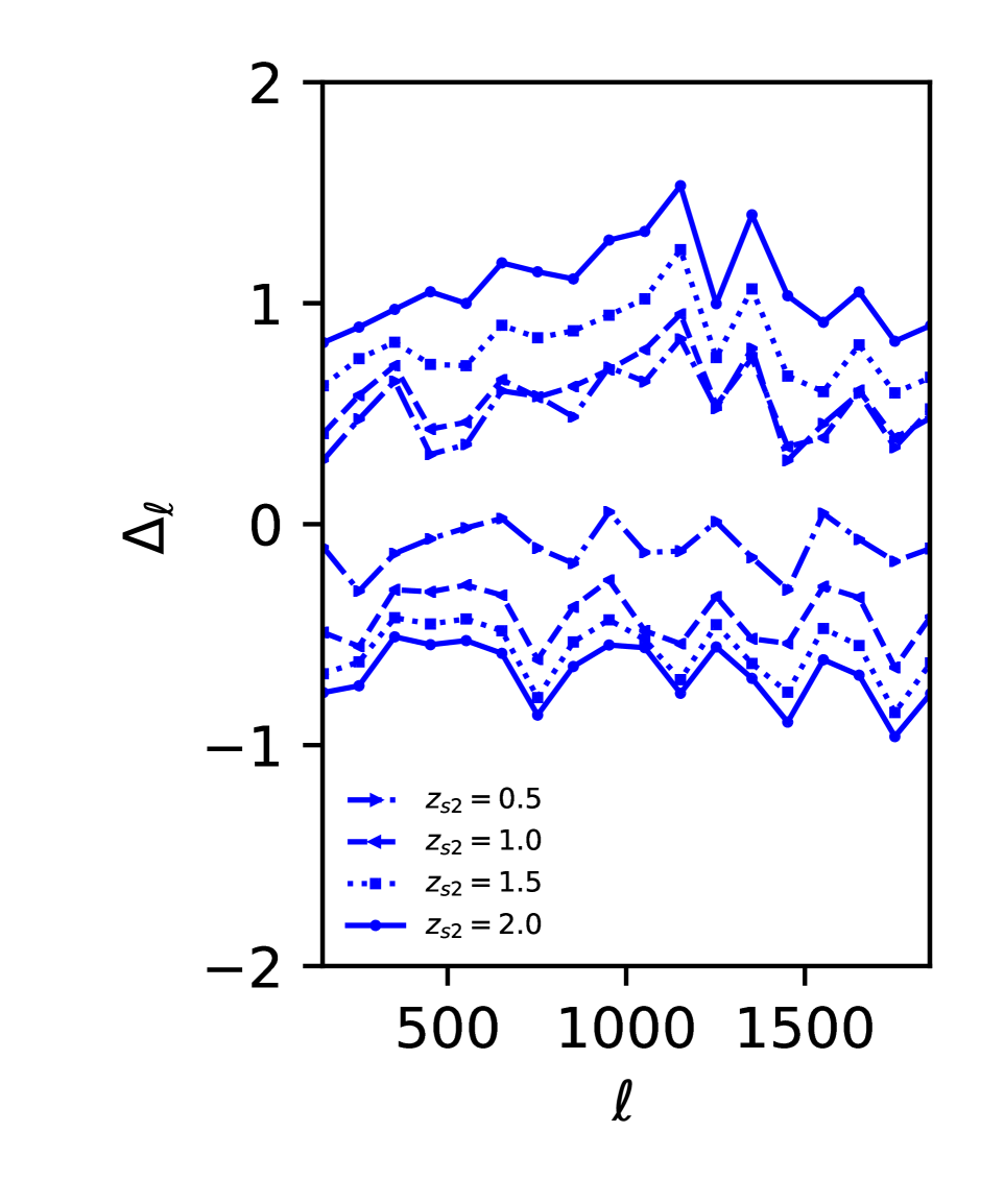
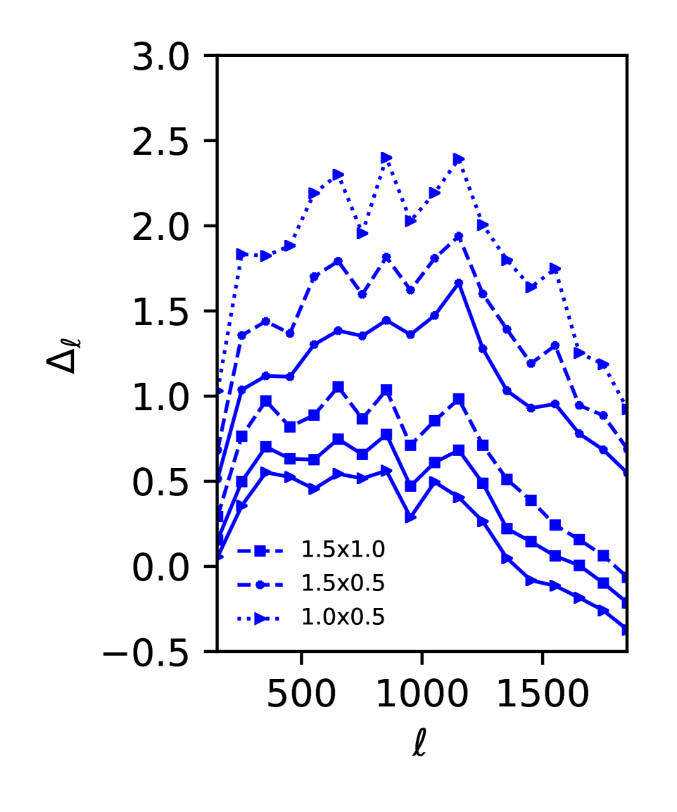
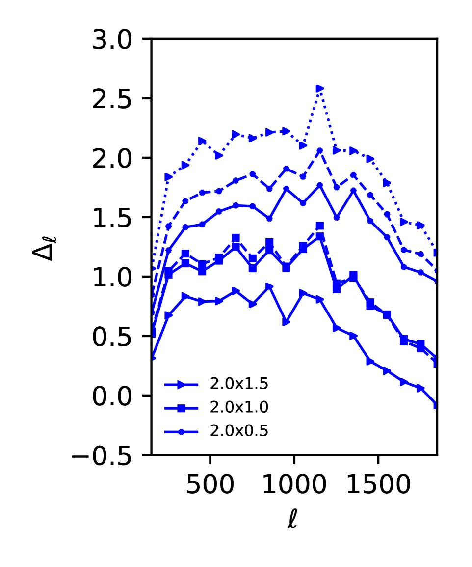
Figure 11: In this figure we present the accuracy of the fitting function we have used in our study. We have used the binned skew-spectra for our comparision. A bin-size of $\delta_{b}=100$ is being used. Here $\Delta_{\ell}$ represents the normalised deviation from predictions and results from simulations (see text for details). The left-panel corresponds to the skew-spectrum computed by cross-correlating the CMB sky and the low redshift weak lensing The middle- and the right-panel correspond to the skew-spectra obtained by cross-correlating two tomographic lensing maps. The plots in the left-panel are obtained using the results presented in the Figure-7 and Figure-8. The upper set of curves correspond to the cross-correlation of tomographic bins against convergence map at $z_{\rm LSS}$ i.e. $\langle\kappa^{2}(z_{s})\kappa_{\rm LSS}\rangle$, whereas the lower curves correspond to their symmetric counterparts $\langle\kappa(z_{s})\kappa^{2}_{\rm LSS}\rangle$. The error in skew-spectra computed using lower redshift maps that are associated with $\langle\kappa^{2}(z)\kappa_{\rm LSS}\rangle$ are depicted in the middel panel. Their symmetric counterparts are shown in the right-panel. The line-styles used in the middle and right panels are identical. For the corresponding skew-spectra see Figure-5 and Figure-6 respectively.

In this paper we have introduced the skew-spectrum statistic as a probe for weak lensing bispectrum. While we found an excellent agreement of numerical simulations and fitting-function based theoretical predictions for the auto-correlation we have studied, we also found significant deviation in many other situations and found that the current analytical uncertainty is not sufficient for high accuracy work. We have primarily focused on gravity induced secondary bispectrum in a $\Lambda$CDM cosmology. However, several extensions of our study are possible.

Skew-spectrum in beyond $\Lambda$CDM scenarios: In most modified gravity theories and dark energy models, the bispectrum is currently known only in the perturbative regime. We have provided analytical expressions for the skew-spectrum in such scenarios. To go beyond perturbative regime a nonlinear model for the bispectrum is required. It is expected that a fitting-function based description in such scenarios will eventually be available as more accurate simulations are performed. Similarly, the modelling of bispectrum based on Effective Field Theories will also be extended to modified gravity theories. Once such results are available, they can readily be used to compute the skew-spectrum in these models.

Higher-order corrections: The theoretical expressions of the skew-spectrum are derived using many simplifying assumptions. We have ignored the corrections due to magnification bias as well as reduced shear which should be included in more accurate theoretical predictions. In addition the skew-spectrum here is computed using the Limber approximation (Kitching et al., 2017).

Skew-spectrum from shear maps: We have computed the skew-spectrum from a convergence map. However, for many practical purposes a skew-spectrum estimated directly from shear maps can bypass many of complications of the map making process.

Intrinsic alignment: The intrinsic alignment (IA) of galaxies (see Vlah, Chisari, Schmidt (1910) and the references therein) are caused by the tidal interaction and is a source of contamination to gravity induced (extrinsic) weak-lensing. The lensing bispectrum induced by IA is typically at the level of $10\%$ of the lensing induced bispectrum. Several methods have been proposed to mitigate or remove such contamination using joint analysis of power-spectrum and bispectrum. The skew-spectrum retains some of the shape information of the original bispectrum. A joint analysis of power spectrum and skew-spectrum can thus be useful in separation of these two different contributions. The skew-spectrum introduced in this study can further be optimised by introducing weights to judge the level of cross-contamination from the intrinsic alignment much in the same way as was achieved in case of point source contamination of CMB studies designed to detect primordial non-Gaussianiaty from Planck data.

Primordial non-Gaussianity and active perturbations: We have considered the gravity induced non-Gaussianity in our study as it is the most dominant source of non-Gaussianity in weak lensing maps. However, similar results can also obtained for computing the sub-dominant contributions from primordial non-Gaussianity as well as secondary sources of non-Gaussianity induced by active sources, e.g., cosmic strings.

Baryonic Feedback: We have not included any baryonic feedback in our modelling of the skew-spectrum but, such corrections can be incorporated in the skew-spectrum for direct comparison with any realistic data.

Covariance and likelihood: We have not discussed the covariance of the skew-spectrum in this study. An accurate description of the covariance will be an important ingredient of cosmological likelihood analysis involving skew-spectrum. A simple form of covariance can be derived under the assumption of Gaussianity and thus ignoring all higher-order correlation contributing to the covariance. Such an estimation will be useful in the noise dominated regime but will not be sufficient in the highly nonlinear scales characterised by high signal-to-noise probed by the future surveys such as Euclid. The methods developed so far in computing the covariance include the ones based on perturbative analysis, halo model or simulated mocks (Rizzato et al., 2019). These methods can be adapted to compute the skew-spectrum covariance.

References

- Allam et al. (2016) The Dark Energy Survey Collaboration, 2016, Phys. Rev. D, 94, 022001
- Amendola et al. (2013) Amendola L. et al. Living Rev. Relativity 16, (2013), 6 [arXiv/1206.1225]
- Assassi (2015) Assassi V., Baumann D., Pajer E., Welling Y. van der Woude D., 2015, JCAP 1511 024, [arXiv/1505.06668]
- Bartolo et al. (2004) Bartolo N., Komatsu E., Matarrese S., Riotto A., 2004, Phys.Rept., 402, 103 [astro-ph/0406398]
- Baumann (2012) Baumann D., Nicolis A., Senatore L., Zaldarriaga M., 2012, JCAP, 1207, 051, [astro-ph/1004.2488]
- de la Bella et al. (2017) de la Bella L. Regan F. D., Seery D., Hotchkiss S., [1704.05309]
- Bellini et al. (2015) Bellini E., Jimenezb R., Verde L., 2015, JCAP, 05, 057 [arXiv/1504.04341]
- Bernardeau (1996) Bernardeau F., 1996, A&A, 312, 11 [astro-ph/9602072]
- Bernardeau et al. (2002) Bernardeau F., Colombi S., Gaztanaga F., Scoccimarro R., 2002, Phys.Rept. 367, 1, [astro-ph/0112551]
- Bernardeau et al. (2002) Bernardeau F., Mellier Y.,van Waerbeke J., 2002, A&A, 389, L28 [astro-ph/0201032]
- Bernardeau et al. (2003) Bernardeau F., van Waerbeke L., Mellier Y., 2003, A&A, 397, 405 [astro-ph/0201029]
- Bernardeau (1994a) Bernardeau F., 1994, Astron.Astrophys. 291, 697 [arXiv/1103.1876]
- Bernardeau (1994b) Bernardeau F. 1994, Astron.Astrophys. 291, 697 [arXiv/1103.1876]
- Bertolini & Solon (2016) Bertolini D., Solon M. P., JCAP 1611 (2016) 030, [1608.01310]
- Calabrese et al. (2018) Calabrese E., J. Smidt J., Amblard, A.,Cooray A., Melchiorri A., Serra P., Heavens A., Munshi D., 2010, PhRvD, 81, 3529 [0909.1837]
- Carrasco, Hertberg, Senatore (2012) Carrasco J. J. M., Hertzberg M. P., Senatore L., JHEP 09 (2012) 082, [astro-ph/1206.2926]
- Clifton et al. (2012) Clifton T., Ferreira P. G., Padilla A., Skordis C., 2012, Physics Reports 513, 1, 1, [astro-ph/1106.2476]
- Codis et al. (2016) Codis S., Pichon C., Bernardeau F., Uhlemann C., Prunet S., 2016, MNRAS, 460, 1549 [arXiv/1603.03347]
- Cooray (2001) Cooray A., 2001, PRD, 64, 043516 [astro-ph/0105415]
- Cooray & Sheth et al. (2002) Cooray A., Sheth R., Phys.Rept.372:1-129,2002, [arxive/0206508]
- Cusina, Lewandowskyi Vernizzi (2018) Cusina G., Lewandowski M., Vernizzi F., 2018, JCAP, 04, 005C [arXiv/1712.02783]
- Dai et al. (2019) Dai J.-P., Verde L., Xia J.-Q., [arXiv/2002.09904]
- Drinkwater et al. (2010) Drinkwater M. J. et al., 2010, MNRAS, 401, 1429 [arXiv/0911.4246]
- Dvali, Gabadadze, Porati (2000) Dvali G., Gabadadze G., Porrati M., 2000, Phys. Rev. B, 485, 208, [arXiv/1510.06930]
- Eisenstein et al. (2011) Eisenstein D. J., Weinberg D. H., Agol E., et al. 2011, AJ, 142, 72, [astro-ph/1101.1529]
- Efsthathiou (2004) Efstathiou G. 2004, MNRAS, 349, 603 [astro-ph/0307515]
- Eggemeier & Smith (2017) Eggemeier A., Smith R. E. 2017, MNRAS, 466, 2496, [arXiv/1603.03347]
- Fabbian, Lewis, Beck (2019) Fabbian G., Lewis A., Beck D., 2019, JCAP, 10, 057 [arXiv/1906.08760]
- Gil-Marin et al. (2011) Gil-Marn H., Wagner C., Fragkoudi F., Jimenez R., Verde L., [arXiv/0902.0618]
-
Gorski et al. (2016)
Gorski K. M., Hivon E., Banday A. J., Wandelt B. D., Hansen F. K.,
Reinecke M., Bartelman M., 2005, ApJ, .622, 759 [astro-ph/0409513] - Gruen et al. (2018) Gruen D., et al., 2018, Phys. Rev. D, 98, 023507 [arXiv/1710.05045]
- Harrison & Coles (2011) Harrison I. , Coles P., 2011, MNRAS, 418, L20, [arXiv/1108.1358]
- Hikage et al. (2011) Hikage C., Takada M., Hamana T., Spergel D., MNRAS, 412, 65, 2011 [arXiv/1004.3542]
-
Hivon et al. (2002)
Hivon E., Gorski K. M., Netterfield B., Crill B. P.,
Prunet S., Hansen F. 2002, ApJ, 567, 2 [astro-ph/0105302] - Joyce et al. (2014) Joyce A., Jain B., Khoury J., Trodden M., 2015, Physics Reports, 568, 1, [astro-ph/1407.0059]
- Kacprzak et al. (2016) Kacprzak T., et al., 2016, MNRAS, 463, 3653 [arXiv/1603.05040]
- Kitching et al. (2017) Kitching T. D., Alsing J., Heavens A. F., Jimenez R., McEwen J. D., Verde L., 2017, MNRAS, 469, 2737, [arXiv/1611.04954]
- Kuijken et al. (2015) Kuijken K., Heymans C., Hildebrandt H., et al. 2015, MNRAS, 454, 3500
- Komatsu, Spergel, Wandelt (2005) Komatsu E., Spergel D. N., Wandelt B. D., 2005, ApJ. 634, 14, [astro-ph/03055189]
- Koyama, Taruya, Hiramatsu (2009) Koyama K., Taruya A., Hiramatsu T. 2009, PRD, 79, 123512, [arXiv/0902.0618]
- Krause et al. (2013) Krause E., Chang T.-C., Doré O., Umetsu K., 2013, ApJ, 762, L20 [arXiv/1210.2446]
- Laureijs et al (2006) Laureijs R., Amiaux J., Arduini S., et al. 2011, ESA/SRE(2011)12
- Lesgourgues & Pastor (2006) Lesgourgues J. , Pastor S. , 2006, Physics Reports, 429, 307, [astro-ph/1610.02956]
- Marques et al. (2018) Marques G. A., Liu J., Zorrilla Matilla J. M., Haiman Z., Bernui A., Novaes C. P., 2019, J. Cosmology Astropart. Phys., 2019, 019 [arXiv/1004.2488]
- Dizgah et al. (2020) Moradinezhad Dizgah A., Lee H., Schmittfull M. Dvorkin C., 2020, JCAP, 04, 011 [arXiv/1911.05763]
- Munshi et al. (2008) Munshi D., Valageas P., Van Waerbeke L., Heavens A., 2008, Physics Reptort, 462, 67 [arXiv:0612667]
- Munshi (2017) Munshi D., 20017, JCAP, 01, 049, [arXiv/1610.02956]
- Munshi (2000) Munshi D. 2000, MNRAS, 318, 145 [astro-ph/0001240]
- Munshi & heavens (2010) Munshi D., Heavens A. 2010, MNRAS, 401, 2406 [astro-ph/0001240]
- Munshi et al. (2011a) Munshi D., Heavens A., Cooray A., Smidt J., Coles P., Serra P., 2011, MNRAS, 412, 1993, [0910.3693]
- Munshi et al. (2011b) Munshi D., Coles P., Cooray A., Heavens A., Smidt J., 2011, MNRAS, 414, 3173, [arXiv/0910.3693]
- Munshi et al. (2011c) Munshi D., Valageas P., Cooray A., Heavens A., 2011, MNRAS, 414, 3173, [arXiv/0910.3693]
- Munshi et al. (2011d) Munshi D., Smidt J., Heavens A., Coles P. , Cooray A., 2011, MNRAS, 411, 2241, [0910.3693]
- Munshi et al. (2018) Munshi D., Coles P., Cooray A., Heavens A. , Smidt J., 2011, MNRAS, 410, 1295, [1002.4998]
- Munshi & Jain (2001) Munshi D., Jain B., 2001, MNRAS, 322, 107 [astro-ph/9912330]
- Munshi & Jain (2000) Munshi D., Jain B,. 2000, MNRAS, 318, 109 [astro-ph/9911502]
- Munshi & Heavens (2010) Munshi D. , Heavens A., 2010, MNRAS, 401, 2406, [astro-ph/0001240]
- Munshi (2000) Munshi D., 2000, MNRAS, 318, 145 [astro-ph/0001240]
- Munshi et al. (2012) Munshi D. , van Waerbeke L., Smidt J., Coles P., 2012, MNRAS, 419, 536 [arXiv/1108.1876]
- Munshi et al. (2019b) Munshi D., McEwen J. D., Kitching T., Fosalba P., Teyssier R., Stadel J., [arXiv/1902.04877]
- Munshi et al. (2019a) Munshi D., Namikawa T., Kitching T. D., McEwen J. D., Takahashi R., Bouchet F. R., Taruya A., Bose, B. [arXiv/1910.04627]
- Munshi et al. (2011e) Munshi D., Kitching T., Heavens A., Coles P. 2011, MNRAS, 416, 629 [arXiv/1012.3658]
- Munshi & McEwen (2020) Munshi D., McEwen J. D. [arXiv/1012.3658]
- Munshi & Regan (2012) Munshi D., Regan D. 2012, JCAP, 06, 042 [arXiv/1705.07666]
- Munshi & McEwen (2020) Munshi D., McEwen J. D., [arXiv/2004.07021]
- National Research Council (2010) National Research Council. 2010. New Worlds, New Horizons in Astronomy and Astrophysics. The National Academies Press. doi:https://doi.org/10.17226/12951
- Namikawa et al. (2018) Namikawa T>, Bose B., Bouchet F. R.,Takahashi R., Taruya A., [arxiv/1812.10635]
- Oh, Spergel, Hinshaw (1990) Oh S. P. Oh, Spergel D. N., Hinshaw G. 1990, ApJ, 510, 551 [astro-ph/9805339]
- Pratten & Munshi (2012) Pratten G., Munshi D., 2012, MNRAS, 423, 4, 3209, [1108.1985]
- Pratten & Lewis (2016) Pratten G., Lewis A. 2016, JCAP, 08, 047 [arXiv/1905.1136]
- Planck Collaboration (2013) Planck Collaboration, 2014, A&A, 571, A16, [astro-ph/1303.5076]
- Planck Collaboration (2015) Planck Collaboration, 2016, A&A 594, A13, [astro-ph/1502.1589]
- Porto et al. (2014) Porto R. A., Senatore L., Zaldarriaga M., JCAP 1405 (2014) 022, [astro-ph/1311.2168]
- Riquelme & Spergel (2018) Riquelme M. A., Spergel D. N., 2007, ApJ, 661, 672, [1002.4998]
- Schmittfull et al. (2015) Schmittfull M., Baldauf T., Seljak U., 2015, PRD, 91, 043530 [arXiv/1411.6595]
- Rizzato et al. (2019) Rizzato M., Benabed K., Bernardeau F., Lacasa F., 2019, MNRAS, 490, 4688 [arXiv/1812.07437]
- Shan et al. (2018) Shan H., et al., 2018, MNRAS, 474, 1116 [arXiv/1805.04114]
- Senatore & Zaldarriaga (2014) Senatore L., Zaldarriaga M., JCAP 1502 (2015) 013, [astro-ph/1404.5954]
- Szapudi et al. (2001) Szapudi I., Prunet S., Pogosyan D., Szalay A. S., Bond J. R., 2001, ApJ, 548, 115 [astro-ph/0010256]
- Smidt et al. (2010) Smidt J., Amblard A., Byrnes C. T., Cooray A., Heavens A., Munshi D. 2010, PRD, 81, 123007 [0909.1837]
- Planck Collaboration (2015) Planck Collaboration, 2016, A&A, 594, 17 [arXiv/1502.01592]
- Planck Collaboration (2018) Planck Collaboration, 2018, [arXiv/1807.06205]
- Scoccimarro & Frieman (1999) Scoccimarro R, Frieman J. A., 1999, ApJ, 520, 35 [astro-ph/9811184]
- Scoccimarro & Couchman (2001) Scoccimarro R., Couchman H. M. P., 2001, MNRAS, 325, 4 [arXiv/0902.0618]
- Takahashi et al. (2017) Takahashi R., Hamana T., Shirasaki M., Namikawa T., Nishimichi T., Osato K., Shiroyama K., 2017, ApJ, 850, 24 [astro-ph/1706.01472]
- Takahasi et al. (2019) Takahashi R., Nishimichi T., Namikawa T., Taruya A., Kayo I., Osato K., Kobayashi Y., Shirasaki M., [arXiv/1911.07886]
- Taylor et al. (2019) Taylor P. L., Kitching T. D., Alsing J., Wandelt B. D., Feeney S. M., McEwen J. D., 2019, Phys. Rev. D 100, 023519 [arXiv/1904.05364]
- Tyson et al. (2003) Tyson J. A., Wittman D. M., Hennawi J. F., Spergel D. N., 2003, Nuclear Physics B Proceedings Supplements, 124, 21
- Uhlemann et al. (2016) Uhlemann C., Codis S., Pichon C., Bernardeau F., Reimberg P., 2016, MNRAS, 460, 1529 [arXiv/1512.05793]
- Valageas (2016) Valageas P., 2002, A&A, 382, 412 [astro-ph/0107126]
- Vlah, Chisari, Schmidt (1910) Vlah Z., Chisari N. E., Schmidt F., [arXiv/1910.08085]
- Weiss et al. (2019) Weiss A. J., Schneider A., Sgier R., Kacprzak T., Amara A., Refregier A., [arXiv/1905.1136]