2D models for MHD flows

Abstract : A new model is proposed for low $Rm$ MHD flows which remain turbulent even in the presence of a magnetic field. These flows minimize the Joule dissipation because of their tendency to become two-dimensional and, therefore to suppress all induction effects. However, some small three-dimensional effects, due to inertia and to the electric coupling between the core flow and the Hartmann layers, are present even within the core flow. This new model, which may be seen as an improvement of the Sommeria-Moreau 2D model, introduces this three-dimensionality as a small perturbation. It yields an equation for the average velocity over the magnetic field lines, whose solution agrees well with available measurements performed on isolated vortices.

Résumé : Un nouveau modèle est proposé pour les écoulements MHD qui demeurent turbulents, même en présence d’un champ magnétique. Ces écoulements minimisent la dissipation par effet Joule en raison de leur tendance à devenir bidimensionnels et, par conséquent, à supprimer tout effet d’induction. Toutefois, la présence d’inertie et le couplage électrique entre les couches de Hartmann et la région centrale maintient certains effets tridimensionnels, même en dehors des couches limites. Ce nouveau modèle, qui peut être vu comme un perfectionnement au modèle antérieur de Sommeria-Moreau, introduit cette faible tridimensionnalité comme une petite perturbation. Il conduit à une équation moyennée sur une ligne de flux magnétique, dont la solution est en bon accord avec des mesures disponibles, effectuées sur des tourbillons isolés.

 

Modèles 2D d’écoulements MHD
(Version française abrégée)

L’action d’un champ magnétique stationnaire et uniforme $\mathbf{B}$ ($Oz,$ vertical) sur un écoulement de fluide conducteur peut se résumer à un phénomène de diffusion qui tend à effacer les différences de vitesses entre plans horizontaux [1]. En première approximation, Lorsque le champ est assez fort, l’écoulement compris entre une plaque et une surface libre (distants de $a$) peut être supposé 2D sauf dans la couche limite voisine de la plaque, où les forces visqueuses sont suffisantes pour équilibrer la force de Lorentz et donner lieu au profil bien connu des couches de Hartmann (d’épaisseur $a/Ha=\left(\rho\nu/\sigma\right)^{1/2}B^{-1}$). Les équations du mouvement moyennées selon la verticale sont donc particulièrement apropriées à la modélisation de ces écoulements. Nous nous proposons d’enrichir ce modèle en y intégrant les effets de l’inertie.

Dans les écoulements 2D, chaque terme de la force de Lorentz, d’ordre $\sigma B^{2}u$ est grand devant tout autre terme de l’équation de Navier Stokes, si bien que les termes habituels d’inertie ne contrôlent pas l’écoulement 2D (désigné par $($ $)^{2D}$ dans la suite).Le courant dans le coeur de l’écoulement est donc nul dans cette première approximation. En fait, un faible courant résulte de l’action des termes habituels de l’équation du mouvement (pression, accélération), petits devant $\sigma B^{2}u$ et qui peuvent donc être construits sur le profil 2D. En conséquence, le courant induit est 2D et par conservation du courant total, il doit être alimenté par un courant vertical linéaire en $z,$ qui implique lui-même un potentiel quadratique en $z$. D’après l’équation (3), le profil de vitesse corrigé $\mathbf{u_{\bot}^{\ast}}$ doit lui aussi être quadratique (6).

Une méthode similaire appliquée à la couche de Hartmann, pour laquelle le premier ordre résulte de l’équilibre entre les forces visqueuses et les forces de Lorentz conduit également à un profil modifié (8). Contrairement à l’approximation classique (sans inertie), ce nouveau profil induit un débit entre coeur et couche limite, caractérisé par l’expression (9).

Connaissant le profil vertical complet, il est désormais possible d’intégrer les équations du mouvement selon $(Oz)$ et d’en déduire une équation d’évolution pour la vitesse horizontale moyennée $\mathbf{\bar{u}}$ entre $z=0$ et $z=a$. Ceci conduit à l’équation (10), où dans un but de simplification, les effets de l’inertie sur le coeur ne sont pas pris en compte. La résolution de cette équation dans la configuration stationnaire et axisymmétrique d’un tourbillon isolé provoqué par une injection de courant ponctuelle située dans le plan $z=0$ permet une comparaison avec les expériences de Sommeria [2] au cours desquelles il a mesuré des profils radiaux de moment cinétique pour de telles structures. Les résultats expérimentaux et analytiques, portés sur la figure 1, sont en accord raisonnable : l’étalement des structures constaté pour des courants d’injection élevés est bien provoqué par un débit de fluide éjecté de la couche de Hartmann au centre du vortex (circulation d’Ekman).

 

1 Introduction.

It is well known since [6] that the action of a steady uniform magnetic field $\mathbf{B}$ on an electrically conducting fluid (conductivity $\sigma,$ density $\rho,$ kinematic viscosity $\nu$) can be seen as a diffusion phenomenon which tends to suppress velocity differences between planes orthogonal to the direction of the magnetic field $\left(Oz\right)$. In the case of a flow bounded by a horizontal plane and a free surface (separated by a distance $a$), a strong enough vertical magnetic field makes this phenomenon dominant (even in comparison with inertial effects) so that the velocity profile does not depend on the $z$ coordinate except within the Hartmann layer located in the vicinity of the wall perpendicular to the field where viscous effect are strong enough to balance the Lorentz force ; the thickness of such layers is $a/Ha$ $=\left(\nu/\sigma\rho\right)^{1/2}B^{-1}$. Averaging the motion equations along   the $z$ direction yields a 2D model which is well adapted to this remarkable flow structure and flexible as it allows any model, such as a turbulent one, for the horizontal flow.

We first review the 2D equation [6] and then look for 3D corrections accounting for non linear behavior of both the Hartmann layer (Ekman-type flows) and the core flow (”barrel” shaped turbulent eddies). Implementing the latter into the motion equation averaged along $\left(Oz\right)$ between $z=0$ and $z=a$ provides an effective 2D model the predictions of which are in good agreement with experiments performed on electrically driven isolated vortices [5].

2 2D models for quasi 2D MHD flows.

In order to describe a weakly 3D flow by a 2D equation of motion , the velocity field is split into its averaged part in the direction of the field $\mathbf{\bar{u}}$ and a departure from this value $\mathbf{u}^{\prime}.$ The Navier-Stokes equation integrated along the field direction writes :

$$(\partial_{t}+\mathbf{\bar{u}.\nabla}_{\bot})\mathbf{\bar{u}}+\overline{\mathbf{u}^{\prime}\mathbf{.\nabla}_{\bot}\mathbf{u}^{\prime}}=-\dfrac{1}{\rho}\mathbf{\nabla}_{\bot}\bar{p}+\nu\mathbf{\Delta}_{\bot}\mathbf{\bar{u}}+\mathbf{\tau}_{W}+\dfrac{\mathbf{u}_{0}}{t_{H}}.$$ (1)

It results from the classical Hartmann layer theory (see for instance [4] p.124-131) that an injected current density $j_{W}$ results in a forcing velocity $\mathbf{u}_{0}=t_{H}B\rho^{-1}\nabla\Psi_{0}\times\mathbf{e}_{z}$ (with $\overline{\mathbf{j}_{\bot}}=\left({at_{H}}\right)^{-1}\nabla\Psi_{0}$ and $\Delta_{\bot}\Psi_{0}=-t_{H}\mathbf{j}_{W}$ where $\overline{\mathbf{j}_{\bot}}$ is the vertically averaged horizontal current density). $t_{H}=a^{2}/\nu 1/Ha$ is the Hartmann damping time which accounts for Joule and viscous dissipations within the Hartmann layer. The subscript ( )_⊥ stands for orthogonal to the field component of vectors. The Lorentz force has then been expressed in function of mechanical quantities thanks to a transformation involving the electric current conservation ([6]).

The averaged quantities, the friction terms and the Reynolds-like tensor appearing in (1) must be derived from a model of the vertical dependance of the velocity. Sommeria and Moreau ([6]) use the classical profile of the Hartmann layer $\mathbf{u}_{h}=\mathbf{u}_{\bot}^{-}\left(1-\exp(-\xi\right))$ (where $\xi=z/Ha$) near the Hartmann wall and the property that in the approximation of strong magnetic field ($Ha$ and $N$ both larger than unity , where $N=a\sigma B^{2}/(\rho U)$ is the ratio of the Lorentz force and the Inertia ) the electromagnetic action is dominant in the balance of forces in the core flow. Then, the velocity profile within the core is not dependent upon the $z$ coordinate (the so called ”2D core model”) and the equation for the average velocity yields :

$$(\partial_{t}+\mathbf{\bar{u}.\nabla}_{\bot})\mathbf{\bar{u}}=-\dfrac{1}{\rho}\mathbf{\nabla}_{\bot}\bar{p}+\nu\mathbf{\Delta}_{\bot}\mathbf{\bar{u}}+\dfrac{1}{t_{H}}\left(\mathbf{u}_{0}-\mathbf{\bar{u}}\right).$$ (2)

The solutions of this equation compare well with explicit linear inertialess 3D solutions in the case of laminar parallel wall side layers ([3]) or isolated vortices aroused by point electrodes ( [2]). But if inertia becomes important, the comparison with available measurements suggests that (2) which is based on a linear vertical velocity profile, has to account for non-linear effects adding a 3D component to the latter.

3 3D phenomena.

3.1 3D effects in the core flow.

Strictly 2D flows are dominated by the balance between the two components of the Lorentz force (respectively the induction part, linked with the motion of the fluid and the electrostatic part) so that no horizontal electric current occurs in the core and the motion is the result of the electrostatic force. In order to improve the 2D approximation, let us consider an additional term in this balance $\mathbf{F}_{\bot}$ ( $=a/\left(l_{\bot}N\right)\left[(\partial_{t}+\mathbf{u.\nabla}_{\bot})\mathbf{u+}\dfrac{1}{\rho}\mathbf{\nabla}_{\bot}p\right]$ if one wants to introduce effects of inertia, where $l_{\bot}$ is a typical horizontal lengthscale ) of smaller order of magnitude which can therefore be assumed to depend only on the 2D velocity profile :

$$\mathbf{F}_{\bot}\mathbf{-}\dfrac{1}{\rho}\mathbf{j}_{\bot}\mathbf{\times B=F}_{\bot}\mathbf{-}\dfrac{\sigma}{\rho}\left(-\mathbf{B}^{2}\mathbf{u_{\bot}+\nabla}_{\bot}\phi\times\mathbf{B}\right)=0.$$ (3)

The right hand side of (3) directly comes from Ohm’s law ($\phi$ is the electric potential). This relation shows that the additional force results in a horizontal current density which is purely divergent if no flow rate comes from the Hartmann layer (Pothérat  et Al. [1]). This current has to be supplied by a vertical current density coming out from the Hartmann layer which is obtained using the current conservation :

$$\sigma\partial_{zz}^{2}\phi=-\mathbf{\nabla}_{\bot}.\mathbf{j}_{\bot}=\rho\left(\mathbf{\nabla}_{\bot}\times\mathbf{F}_{\bot}\right).\mathbf{B.}$$ (4)

As $\mathbf{j}_{\bot}$ and are $z$ independent, this variation of potential along the magnetic field lines induces a quadratic dependence upon $z$ for the vertical profile of velocity in (3) :

$$\partial_{zz}^{2}\mathbf{u}_{\bot}=\dfrac{\rho}{\sigma}\mathbf{\nabla}_{\bot}\times\mathbf{\nabla}_{\bot}\times\mathbf{F}_{\bot}.$$ (5)

This demonstrates that the velocity cannot be 2D anymore so that the well-known 2D vortices do not look like columns anymore but rather like ”barrels” :

$$\mathbf{u_{\bot}}\left(z\right)\mathbf{=u}_{\bot}^{-}+\dfrac{z}{2}\left(z-\dfrac{2a}{n}\right)\dfrac{a^{2}}{\nu}\dfrac{N}{Ha^{2}}\mathbf{\nabla}_{\bot}\times\mathbf{\nabla}_{\bot}\times\mathbf{F}_{\bot}$$ (6)

Notice that if no flow rate occurs at the bottom (or the top) of the eddies, this 3D mechanism induces no additional vertical flow.

3.2 Inertial effects in the Hartmann layer.

In the Hartmann layer, the viscous force is of the same order as the Lorentz force so that the usual exponential leading order profile is already the result of a balance between both of them and the pressure gradient. In order to introduce the effects of inertia as a small perturbation, for instance to account for a big vortex standing over the layer, an additional inertial term has to be added  whose $\xi$ dependance comes from this profile. The motion equation of within such a layer can be written :

$$a/\left(Nl_{\bot}\right)\left[\partial_{t}+\mathbf{u}_{\bot}^{-}\left(1-\exp\left(-\xi\right)\right)\mathbf{.\nabla}_{\bot}\right]\mathbf{u}_{\bot}^{-}\left(1-\exp\left(-\xi\right)\right)\mathbf{=}\\ \mathbf{-}\dfrac{1}{\rho}\mathbf{\mathbf{\nabla}_{\bot}}p-\dfrac{\sigma}{\rho}\mathbf{\nabla}_{\bot}\phi\times\mathbf{B}-\dfrac{\sigma}{\rho}\mathbf{B}^{2}\mathbf{u}_{h}\left(\xi\right)\mathbf{+}\nu\partial_{zz}^{2}\mathbf{u}_{h}\left(\xi\right).$$ (7)

Since the pressure and the electric potential do not vary at the scale of the Hartmann layer, after a straightforward integration, we get :

$$\mathbf{u}_{h}\left(\xi\right)=\mathbf{u}_{\bot}^{-}\left(1-\exp\left(-\xi\right)\right)\\ +\dfrac{t_{H}}{Ha}\left[\left(\dfrac{1}{3}e^{-2\xi}-\dfrac{1}{3}e^{-\xi}+\xi e^{-\xi}\right)\mathbf{u}_{\bot}^{-}.\nabla_{\bot}\mathbf{u}_{\bot}^{-}+\dfrac{1}{2}\xi e^{-\xi}\partial_{t}\mathbf{u}_{\bot}^{-}\right].$$ (8)

It is noticeable that this profile is not divergent-free so that it implies some flow rate between the Hartmann layer and the core flow. The vertical velocity at the interface of the two regions $w^{-}$ is derived from the mass conservation :

$$w_{h}^{-}=-\dfrac{5}{6}\dfrac{at_{H}}{Ha^{2}}\mathbf{\nabla}_{\bot}.\left(\mathbf{u}_{\bot}^{-}\mathbf{.\nabla}_{\bot}\mathbf{u}_{\bot}^{-}\right)$$ (9)

It should be noticed too that this behavior is not dependent upon the electric conditions at the Hartmann walls.

4 Application to the case of isolated vortices.

Using the models of the previous paragraph for the velocity profile in both the Hartmann layer and the core flow, it is possible to express $\mathbf{u}_{\bot}^{-}$ in function of $\mathbf{\bar{u}}$ and to assess $\mathbf{\tau}_{W}$ and $\overline{\mathbf{u}^{\prime}\mathbf{.\nabla}_{\bot}\mathbf{u}^{\prime}}$ in (1) to obtain a 2D equation accounting for 3D inertial phenomena. In order to get a simple model, we limit ourselves to the inertial effects in the Hartmann layer and we neglect the core ”barrel effect” corrections are taken on account. It can be checked that this becomes exact in axisymmetric configurations. Under this assumptions, (1) yields :

$$\dfrac{d\mathbf{v}}{dt^{\prime}}+\mathbf{\nabla}_{\bot}\bar{p}^{\prime}=\nu\mathbf{\Delta}_{\bot}\mathbf{v-}\dfrac{1}{t_{H}}\left(\mathbf{v}_{0}-\alpha\mathbf{v}\right)\mathbf{+}\dfrac{t_{H}}{Ha^{2}}\left(\dfrac{7}{36}\mathcal{D}_{\mathbf{v}}+\dfrac{1}{8}\partial_{t}\right)\mathbf{v}.\mathbf{\nabla}_{\bot}\mathbf{v}$$ (10)

where $\alpha=1+1/Ha,$ $\mathbf{v}$ (resp. $\mathbf{v}_{0}$, resp. $\bar{p}^{\prime}$)$.\mathbf{=}\left(1+7/\left(6Ha\right)+11/6Ha^{2}\right)\mathbf{\bar{u}}$ (resp. $\mathbf{u}_{0}$, resp. $\bar{p}$), $\partial t^{\prime}=\left(1+1/Ha+n^{2}/Ha^{2}\right)\partial t$ and $\mathcal{D}_{\mathbf{v}}$ stands for the operator $\mathcal{D}_{\mathbf{v}}:\mathbf{F\longmapsto}\mathcal{D}_{\mathbf{v}}\mathbf{F=}\left(\mathbf{v.\nabla}_{\bot}\right)\mathbf{F+}\left(\mathbf{F.\nabla}_{\bot}\right)\mathbf{v.}$

This model may be checked by comparison of its results for isolated vortices with the measurements performed by Sommeria ([5]). His experimental device consists in a cylindrical tank (radius $60$ mm) filled with a layer of mercury (depth $19.2$ mm) at the center of which an electric current is injected via a point electrode located at the bottom. The upper surface is free so that the velocities are derived from streak photos of particles conveyed by the fluid.

In this configuration, if $I$ is the injected electric current, the forcing expresses as ([5]) :

$$u_{0\theta}=\dfrac{\Gamma}{r}\text{ \ with \ }\Gamma=\dfrac{I}{2\pi\sqrt{\rho\sigma\nu}}.$$ (11)

so that the equation can be rewritten in steady axisymmetric configuration and using non-dimensional variables $r_{\dim}=r\sqrt{\nu t_{H}/\alpha}$ and $u_{\theta\dim}=u_{\theta}\Gamma/a\sqrt{\alpha Ha}$ :

$$C_{t}\dfrac{1}{r^{2}}\partial_{r}\left(ru_{\theta}^{3}\right)=\dfrac{1}{r^{2}}\partial_{r}\left[r^{3}\partial_{r}\left(\dfrac{u_{\theta}}{r}\right)\right]-u_{\theta}+\dfrac{1}{r},$$ (12)

with the corresponding boundary conditions :

$$u_{\theta}\left(R\right)=0\text{and}\underset{r\rightarrow+\infty}{\lim}u_{\theta}=0.$$ (13)

In (12) $C_{t}=\dfrac{7}{36}\left(1+\dfrac{1}{Ha}\right)^{3/2}\dfrac{1}{N_{c}^{2}}$ where $N_{c}=\dfrac{\sigma B^{2}}{\rho}\dfrac{a^{2}}{\Gamma Ha}$ , the interaction parameter scaled on the solid core of the vortex ([5]) appears as the relevant parameter for this problem. We have performed numerical simulations of (12) for two different values of the injected current ($I=50mA$ and $I=200mA$ respectively corresponding to $C_{t}=8.85$ and $C_{t}=141.65$ ). The results are reported on figure (1). A satisfactory agreement is found between theory and experiment. It turns out that the core of the vortices actually broadens for increasing values of the injected current (i.e. when inertia becomes important). This phenomenon can be interpreted as an Ekman recirculation : the flow rate between the Hartmann layer and the core (9) is related to the spatial variation of the centrifugal acceleration of the fluid, which is strong and positive at the center of the vortex  (strong flow towards the core) and negative and weak at long distance of the center. This toroidal flow is an MHD equivalent of the Ekman pumping.

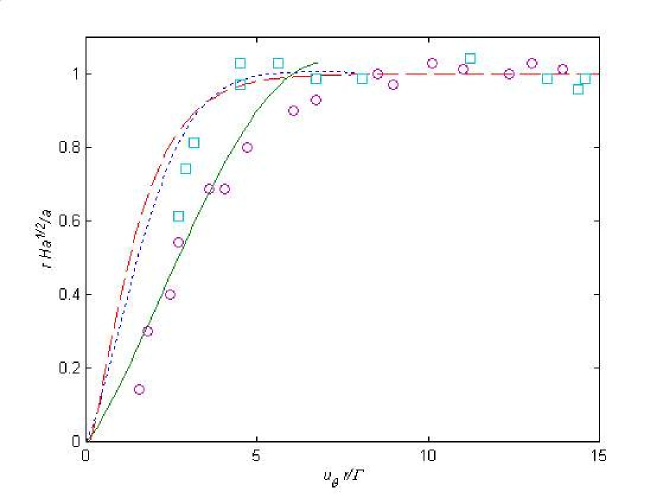
Figure 1: Vortex radial profile of angular momentum for $B=0.5$ T: boxes: experimental measurements for injected current $I=0.05$ A, circles: experimental measurements for $I=0.2$ A, full line: analytical profile without non linear effects, semi dotted line: numerical profile for $I=0.05$ A, dotted line: numerical profile for $I=0.2$ A. Note that numerical precision problems don’t allow to get to profiles for any values of r. Profil radial de moment cinétique de tourbillons isolés pour $B=0.5T$ : (carrés) : Mesures expérimentales pour un courant de $I=0.05A,$ ronds : mesures epérimentales pour $I=0.2A,$ ligne pleine : courbe analytique sans effet non linéaire, ligne interrompue : courbe numérique à $I=0.05A$, pointillés : courbe numérique à $I=200A$.

References

- [1] A. Pothérat, J. Sommeria and R. Moreau 2000 An effective two-dimensional model for MHD flows with transverse magnetic field. J. Fluid Mech. 424, 75–100.
- [2] J. C. R. Hunt and W. E. Williams 1968 Some electrically driven flows in magnetohydrodynamics. part1. theory. J. Fluid. Mech. 314, 705–722
- [3] A. Shercliff 1953 Proc. Camb. Phil. Soc. 49, 136
- [4] R. Moreau 1990 Magnetohydrodynamics Kluwer Acad. Pub. Dordrecht
- [5] J. Sommeria 1988 Electrically driven vortices in a strong magnetic field. J. Fluid. Mech. 189, 553–569
- [6] J. Sommeria and R. Moreau 1982 Why, how and when turbulence becomes two-dimensional. J. Fluid. Mech. 118, 507–518