Resonating AdS soliton

Abstract

The AdS soliton is a nonsingular spacetime that has a flat conformal boundary with a compact $S^{1}$ direction. We find a horizonless cohomogeneity-1 metric that describes nonlinear gravitational oscillations of the AdS soliton in five dimensions. We call this spacetime the resonating AdS soliton. This solution is obtained as the nonlinear extension of normal modes of the AdS soliton dual to spin-2 glueball excitations. The boundary energy momentum tensor of the resonating AdS soliton has time periodic components, and it is interpreted as a coherently excited state in the dual field theory. Physical quantities of the resonating AdS soliton are multivalued at a fixed energy, suggesting a transition between different frequency solutions. The energy of the resonating AdS soliton is higher than that of the undeformed AdS soliton, in accordance with the positive energy conjecture proposed by Horowitz and Myers.

1 Introduction

The AdS soliton Horowitz:1998ha is a globally non-singular solution that has negative energy relative to the pure AdS space. It is an asymptotically locally AdS spacetime and has a flat conformal boundary with a compact $S^{1}$ circle. It has been conjectured that the AdS soliton is the unique lowest energy solution among the spacetimes with the same asymptotic structure Horowitz:1998ha ; Constable:1999gb . The uniqueness theorem for the AdS soliton supports the conjecture Galloway:2001uv ; Galloway:2002ai , but its full proof is yet to be given Woolgar:2016axs .

In the AdS/CFT duality Maldacena:1997re ; Gubser:1998bc ; Witten:1998qj , the AdS soliton has been considered with respect to the gravity dual of the confining phase of pure Yang-Mills theory. In the dual field theory, an anti-periodic boundary condition for fermions along the $S^{1}$ breaks supersymmetry, and so pure Yang-Mills theory can be described Witten:1998zw . In the bulk, the spacetime of the AdS soliton is smoothly capped at a finite distance where the $S^{1}$ shrinks, and gapped normal modes, corresponding to the confined spectrum, are obtained. At finite temperature, there is a Hawking-Page transition Hawking:1982dh between an AdS soliton and a black brane Surya:2001vj , and this is interpreted as the confinement/deconfinement transition Witten:1998zw .

In this paper, we will study time-periodic states in the confined phase of the gauge theory by using its gravity dual. Understanding dynamical phenomena is one of the most challenging problems of strongly coupled quantum many body systems. The gauge/gravity duality helps us to understanding such problems. The normal modes that the AdS soliton admits are expected to have a nonlinear extension. In particular, we will focus on the spin-2 perturbation of the AdS soliton Constable:1999gb ; Brower:1999nj and show that its nonlinear extension leads to a non-stationary time periodic solution. We will call such solutions as the resonating AdS solitons.

In particular, we will consider five-dimensional solutions with cohomogeneity-1 metrics. In asymptotically global AdS space, similar setups for non-stationary solutions have been considered. Solutions describing nonlinear gravitational oscillations are called geons Dias:2011ss ; Horowitz:2014hja ; Martinon:2017uyo ; Fodor:2017spc . Analogously, there are boson stars, characterized by oscillating scalar fields Dias:2011at ; Liebling:2012fv ; Maliborski:2013jca ; Buchel:2013uba ; Fodor:2015eia ; Choptuik:2017cyd ; Choptuik:2018ptp . These solutions are non-stationary but time periodic. Geons constructed in four dimensions only have a single helical Killing vector Horowitz:2014hja . But recently, by going to five dimensions, geons whose metric is cohomogeneity-1 (i.e. the metric functions only depend on a single variable) have been constructed Ishii:2018oms ; Ishii:2019wfs . By applying techniques in Refs. Ishii:2018oms ; Ishii:2019wfs , we construct the resonating AdS soliton with cohomogeneity-1 metric in five dimensions. There has been a perturbative construction Hartnett:2012np , but we are able to find non-trivial nonlinear solutions.

Gravitational dynamics in AdS space of general relativity is theoretically interesting. Because of the timelike conformal boundary of the asymptotically AdS space, non-trivial dynamics can be realized. One example is the weakly turbulent instability of global AdS space Bizon:2011gg : pure AdS is nonlinearly unstable against arbitrarily small perturbations, and a black hole is formed for a wide class of initial data. Similar phenomena has been observed in the AdS soliton background although the presence of a finite threshold of amplitude for the black hole formation is a significant difference Craps:2015upq ; Myers:2017sxr . Below the threshold, the spacetime oscillates forever and is time periodic. Our resonating AdS soliton might be one simple realization of such a phase.

The normal modes of the AdS space are connected to the onset of the superradiant instability of rotating black holes Hawking:1999dp ; Reall:2002bh ; Cardoso:2004hs ; Kunduri:2006qa ; Cardoso:2006wa ; Murata:2008xr ; Kodama:2009rq ; Dias:2011at ; Dias:2013sdc ; Cardoso:2013pza . Indeed, gravitational geons correspond to the smooth horizonless limit of black resonators Dias:2015rxy ; Niehoff:2015oga ; Ishii:2018oms ; Ishii:2019wfs . A black resonator is a dynamical spacetime. Therefore, it will be prone to further superradiant instabilities Green:2015kur . Stability analysis has been carried out for five-dimensional cohomogeneity-1 solutions Ishii:2020muv , and cascades of instabilities are expected, but their endpoint is an open problem Niehoff:2015oga . A study of such of nonlinear evolution is Chesler:2018txn .

In holography, time periodic states have been studied by applying periodic driving by external sources at the conformal boundary Li:2013fhw ; Natsuume:2013lfa ; Auzzi:2013pca ; Rangamani:2015sha ; Hashimoto:2016ize ; Kinoshita:2017uch ; Biasi:2017kkn ; Ishii:2018ucz ; Biasi:2019eap . Such time dependent solutions provide a time dependent oscillating condensate called Floquet condensate in the dual field theory. In the presence of a black hole horizon, the driving can be dissipated; when a horizon is absent, resonances can be excited. These driven states survive in the limit of zero source amplitude, resulting in spontaneously excited states which nonlinearly extend the normal modes. In this paper, we directly construct cohomogeneity-1 solutions without applying a nontrivial boundary source.

This paper is organized as follows. In Section 2, we study spin-2 normal modes of the AdS soliton. In Section 3, we set up the nonlinear extension of the normal modes. Numerical results for the resonating AdS soliton are presented in Section 4. This paper is concluded with a summary and discussion in Section 5.

2 Normal modes of AdS soliton

2.1 AdS soliton

We consider five dimensional Einstein gravity with a negative cosmological constant,

$$R_{\mu\nu}-\frac{1}{2}g_{\mu\nu}R=\frac{6}{L^{2}}g_{\mu\nu}\ ,$$ (1)

where $L$ is the AdS radius. We will set $L=1$ throughout this paper.

The AdS soliton is a solution to the Einstein equation (1) with a flat conformal boundary:

$$ds^{2}=\frac{1}{z^{2}}\left[-dt^{2}+\frac{dz^{2}}{F(z)}+\frac{z_{0}^{2}}{4}F(z)d\theta^{2}+dx^{2}+dy^{2}\right]\ ,\quad F(z)=1-\frac{z^{4}}{z_{0}^{4}}\ .$$ (2)

This metric can also be obtained by the double Wick rotation of the Schwarzschild-AdS₅ solution with a flat horizon Horowitz:1998ha . The AdS boundary is located at $z=0$. The coordinate $\theta$ is compactified on a circle with a periodicity $\theta\simeq\theta+2\pi$ in order to avoid a conical singularity at the tip of the geometry where $z=z_{0}$. This geometry contains 3d Minkowski space denoted by $-dt^{2}+dx^{2}+dy^{2}$ and is invariant under $ISO(2,1)$. It is also invariant under a $\theta$-translation. In summary, the isometry group of the AdS soliton is

$$ISO(2,1)\times U(1)\ .$$ (3)

For later convenience, we denote the generator of the rotation in the $(x,y)$-plane by

$$\xi=x\frac{\partial}{\partial y}-y\frac{\partial}{\partial x}\ .$$ (4)

This is the generator of $U(1)\in ISO(2,1)$.

The compactified direction introduces the Kaluza-Klein mass scale $M_{KK}$. Near the AdS boundary $z\sim 0$, the metric (2) becomes

$$ds^{2}\simeq\frac{1}{z^{2}}\left[-dt^{2}+dx^{2}+dy^{2}+\frac{z_{0}^{2}}{4}d\theta^{2}\right]\ .$$ (5)

The boundary metric is locally 4d Minkowski, but the $\theta$-direction is compactified. For the AdS soliton, the Kaluza-Klein mass scale is given by

$$M_{KK}=\frac{2}{z_{0}}\ .$$ (6)

In this paper, we will measure dimensionful quantities in units of $M_{KK}$.

2.2 Decoupled spin-2 perturbation

We focus on the decoupled spin-2 gravitational perturbation of the AdS soliton that is homogeneous in the $(x,y)$-plane Constable:1999gb ; Brower:1999nj . Here, we also include a nontrivial Kaluza-Klein momentum $k$ along the $\theta$-coordinate. We formulate the perturbation in a way that will naturally leads to the nonlinear construction in the following section.

Let us introduce complex coordinates $w_{\pm}$ in the $(x,y)$-plane as

$$dw_{\pm}=dx\pm idy\ .$$ (7)

These satisfy

$$\mathcal{L}_{\xi}dw_{\pm}=\pm idw_{\pm}\ ,$$ (8)

where $\mathcal{L}$ is the Lie derivative. This means that $dw_{\pm}$ have $U(1)$-charges of $\pm 1$. Then we consider the following gravitational perturbation of the AdS soliton:

$$h_{\mu\nu}dx^{\mu}dx^{\nu}=\frac{1}{z^{2}}e^{-i\omega t+ik\theta}\delta\alpha(z)dw_{+}^{2}+\textrm{h.c.}\ .$$ (9)

From the periodicity of $\theta$, $k\in\bm{Z}$ is required. This perturbation has $U(1)$-charges of $+2$ (first term) and $-2$ (second term), and it is homogeneous in the $(x,y)$-plane: $\partial_{x}h_{\mu\nu}=\partial_{y}h_{\mu\nu}=0$. Other homogeneous perturbations such as $dt^{2},\,dtdw_{+}$, and $dzdw_{-}$ cannot have $U(1)$-charges of $\pm 2$. Thus the perturbation (9) is decoupled from the other perturbations.

The perturbation equation for $\delta\alpha$ is given by

$$\delta\alpha^{\prime\prime}+\frac{(z^{-3}F)^{\prime}}{z^{-3}F}\delta\alpha^{\prime}+\left(\frac{\omega^{2}}{F}-\frac{4k^{2}}{z_{0}^{2}F^{2}}-\frac{2(zF^{\prime}-4F+4)}{z^{2}F}\right)\delta\alpha=0\ .$$ (10)

Solving the above equation near the tip $z=z_{0}$ and conformal boundary $z=0$, we find the regular and Dirichlet boundary conditions as

$$\delta\alpha\sim(z_{0}-z)^{k/2}\quad(z\sim z_{0})\ ,\qquad\delta\alpha\sim z^{4}\quad(z\sim 0)\ .$$ (11)

We compute the normal mode spectrum for $\omega$ by solving (10) numerically with these boundary conditions. Results are summarized in Table 1. There, $n$ denotes the radial overtone number given by the number of nodes in the interval $0\leq z\leq z_{0}$ and corresponds to the excitations of the dual spin-2 glueballs Constable:1999gb ; Brower:1999nj . The numerical values for $k=0$ reproduce the spectrum obtained in Csaki:1998qr ; deMelloKoch:1998vqw ; Zyskin:1998tg for $0^{++}$ glueballs, which degenerate with the $2^{++}$ glueball spectrum Constable:1999gb ; Brower:1999nj .

Table 1: The spectrum of the gravitational perturbation $\omega/M_{KK}$.

	$n=0$	$n=1$	$n=2$	$n=3$
$k=0$	1.7020	2.9380	4.1526	5.3598
$k=1$	2.4224	3.6144	4.8082	6.0034
$k=2$	3.2544	4.3848	5.5424	6.7139
$k=3$	4.1412	5.2130	6.3309	7.4740
$k=4$	5.0587	6.0788	7.1580	8.2717

3 Nonlinear resonation of AdS soliton

3.1 Symmetry preserved by the perturbation

The main goal of this paper is to construct nonlinear solutions that extend from the normal modes obtained in the previous section. In this section, we identify the metric ansatz for the nonlinear solutions and set up its computation. A perturbative construction has been given in Hartnett:2012np , but here we will construct complete nonlinear solutions. In particular, we find that they are obtained in a cohomogeneity-1 metric ansatz.

To find the metric ansatz for the nonlinear solutions, we examine the symmetries preserved by the perturbation (9). Let us define the following 1-forms $e_{\pm}$ by

$$e_{\pm}=e^{\pm(-i\omega t+ik\theta)/2}dw_{\pm}\ .$$ (12)

In terms of them, the perturbation (9) is simply written as

$$h_{\mu\nu}dx^{\mu}dx^{\nu}=\frac{1}{z^{2}}\delta\alpha(z)(e_{+}^{2}+e_{-}^{2})\ .$$ (13)

Hence it is convenient to look at the symmetries acting on $e_{\pm}$. The 1-forms $e_{\pm}$ are transformed by $\xi$, $\partial_{t}$ and $\partial_{x}$ as

$$\mathcal{L}_{\xi}e_{\pm}=\pm ie_{\pm}\ ,\quad\mathcal{L}_{\partial_{t}}e_{\pm}=\mp\frac{i\omega}{2}e_{\pm}\ ,\quad\mathcal{L}_{\partial_{\theta}}e_{\pm}=\pm\frac{ik}{2}e_{\pm}\ .$$ (14)

The $t$ and $\theta$-translations are broken if $\omega\neq 0$ and $k\neq 0$, respectively, but their linear combinations with $\xi$ are preserved, defining vector fields $K_{1}$ and $K_{2}$ by

$$K_{1}=\partial_{t}+\frac{\omega}{2}\xi\ ,\qquad K_{2}=\partial_{\theta}-\frac{k}{2}\xi\ ,$$ (15)

implying that

$$\mathcal{L}_{K_{1}}e_{\pm}=0\ ,\qquad\mathcal{L}_{K_{2}}e_{\pm}=0\ .$$ (16)

Thus, the perturbation (13) preserves the symmetries generated by $K_{1}$ and $K_{2}$. That is, $\xi$, $\partial_{t}$ and $\partial_{x}$ are not Killing vectors independently, but their appropriate linear combinations are. In $K_{1}$, the $t$-translation is combined with the rotation generated by $U(1)_{\xi}$, and therefore $K_{1}$ can be regarded as a helical Killing vector. The 1-forms $e_{\pm}$ are also invariant under translations in the $(x,y)$-plane: $\mathcal{L}_{\partial_{x}}e_{\pm}=\mathcal{L}_{\partial_{y}}e_{\pm}=0$. The upshot is that the perturbation (13) is invariant under $\{K_{1},K_{2},\partial_{x},\partial_{y}\}$.

What is the isometry group generated by $\{K_{1},K_{2},\partial_{x},\partial_{y}\}$? To identify that, it is more appropriate to consider $L_{1}\equiv 2K_{1}/\omega=\xi+(2/\omega)\partial_{t}$ and $L_{2}\equiv kK_{1}+\omega K_{2}=k\partial_{t}+\omega\partial_{\theta}$ so that $\xi$ and $\partial_{\theta}$ are separated. Clearly, $\mathcal{L}_{L_{1}}e_{\pm}=0=\mathcal{L}_{L_{2}}e_{\pm}$. Recall that $\{\xi,\partial_{x},\partial_{y}\}$ form the algebra of $ISO(2)$, although $\xi$ is no longer a Killing vector. Then, because $[\partial_{t},\partial_{x}]=[\partial_{t},\partial_{y}]=0$, we can say that $\{L_{1},\partial_{x},\partial_{y}\}$ are the generators of $ISO(2)$. The remaining one $L_{2}$ commutes with the other vectors $\{L_{1},\partial_{x},\partial_{y}\}$ and is the generator of $U(1)$ for $k=0$ and $R$ for $k\neq 0$. Thus, the isometry group generated by $\{K_{1},K_{2},\partial_{x},\partial_{y}\}$ is given by

$$\begin{split}&ISO(2)\times U(1)\qquad(k=0)\ ,\\ &ISO(2)\times R\qquad(k\neq 0)\ .\end{split}$$ (17)

The original isometry group of the AdS soliton (3) is broken into these smaller groups by the perturbation (13).

The perturbation (13) is also invariant under discrete transformations $P_{1}$ and $P_{2}$ given by

$$\begin{split}&P_{1}(t,\theta,x,y)=(-t,-\theta,-x,y)\ ,\\ &P_{2}(t,\theta,x,y)=(-t,-\theta,x,-y)\ .\end{split}$$ (18)

Under these, 1-forms $(dt,d\theta,e_{+},e_{-})$ are transformed as

$$\begin{split}&P_{1}(dt,d\theta,e_{+},e_{-})=(-dt,-d\theta,-e_{-},-e_{+})\ ,\\ &P_{2}(dt,d\theta,e_{+},e_{-})=(-dt,-d\theta,e_{-},e_{+})\ .\end{split}$$ (19)

3.2 Metric for resonating AdS soliton

We will now construct the metric ansatz that has Killing vectors $\{K_{1},K_{2},\partial_{x},\partial_{y}\}$. To this end, it is convenient to introduce real 1-forms $e_{1}$ and $e_{2}$ as

$$e_{\pm}=e_{1}\pm ie_{2}\ .$$ (20)

They can be related to the original orthogonal coordinates, $(x,y)$, as

$$\begin{pmatrix}e_{1}\\ e_{2}\end{pmatrix}=\begin{pmatrix}\cos\Theta&-\sin\Theta\\ \sin\Theta&\cos\Theta\end{pmatrix}\begin{pmatrix}dx\\ dy\end{pmatrix}\ ,\qquad\Theta=\frac{1}{2}(-\omega t+k\theta)\ .$$ (21)

These are also invariant under $\{K_{1},K_{2},\partial_{x},\partial_{y}\}$. Then, we can write a general metric equipped with them as

$$ds^{2}=g_{ab}(z)E^{a}E^{b}\ ,$$ (22)

where $E^{a}=(dt,dz,d\theta,e_{1},e_{2})$. The metric depends only on $z$ but still has 15 components. This can be further simplified by imposing the parity (19), under which $(dt,d\theta,e_{1},e_{2})$ are transformed as

$$\begin{split}&P_{1}(dt,d\theta,e_{1},e_{2})=(-dt,-d\theta,-e_{1},e_{2})\ ,\\ &P_{2}(dt,d\theta,e_{1},e_{2})=(-dt,-d\theta,e_{1},-e_{2})\ .\end{split}$$ (23)

Therefore, in Eq. (22), only the terms with $dt^{2},\,dtd\theta,\,d\theta^{2},\,dz^{2},\,e_{1}^{2},$ and $e_{2}^{2}$ are allowed if the parity invariance is imposed. This leads us to write the cohomogeneity-1 metric ansatz as

$$ds^{2}=\frac{1}{z^{2}}\bigg{[}-f(z)dt^{2}+\frac{dz^{2}}{F(z)g(z)}+\alpha(z)e_{1}^{2}+\frac{1}{\alpha(z)}e_{2}^{2}\\ +\frac{z_{0}^{2}}{4}F(z)\beta(z)\{d\theta-h(z)dt\}^{2}\bigg{]}\ ,$$ (24)

where $F(z)$ was defined in Eq. (2). The product of the coefficients of $e_{1}^{2}$ and $e_{2}^{2}$ are fixed by redefinition of the $z$-coordinate. Note that a similar metric has also appeared as an effective metric on the probe D7-brane when a rotating electric field is applied in the D3/D7 system Hashimoto:2016ize ; Kinoshita:2017uch . To avoid a conical singularity at the tip, we require

$$g(z)\beta(z)|_{z=z_{0}}=1\ .$$ (25)

The AdS soliton (2) is reproduced when $f=g=\alpha=\beta=1$ and $h=0$.

Substituting the ansatz (24) into the Einstein field equation $G_{\mu\nu}=6g_{\mu\nu}$, we obtain the complete set of the equations of motions as

$$f^{\prime}= \frac{1}{4z_{0}^{2}zFg\alpha^{2}\{z(F\beta)^{\prime}-6F\beta)\}}\big{[}z_{0}^{2}F\{z^{2}Fg\beta(-z_{0}^{2}Fh^{\prime}{}^{2}\alpha^{2}\beta+4\alpha^{\prime}{}^{2}f)$$

$$+24zfg\alpha^{2}(F\beta)^{\prime}-96f\alpha^{2}\beta(Fg-1)\}$$

$$+z^{2}(\alpha^{2}-1)^{2}\{z_{0}^{2}F\beta(\omega-kh)^{2}-4k^{2}f\}\big{]}\ ,$$ (26)

$$g^{\prime}= \frac{1}{4z0^{2}zFf\alpha^{2}\beta(z(F\beta)^{\prime}-6F\beta)}\big{[}-z_{0}^{2}\{z^{2}g\alpha^{2}\beta^{2}(-z_{0}^{2}F^{3}h^{\prime}{}^{2}\beta+8F^{\prime}{}^{2}f)$$

$$+4zF^{\prime}Ffg\alpha^{2}\beta(3z\beta^{\prime}-14\beta)+4z^{2}F^{2}fg(\alpha^{2}\beta^{\prime}{}^{2}+\alpha^{\prime}{}^{2}\beta^{2})$$

$$+32zf\alpha^{2}\beta(-F^{2}g\beta^{\prime}+(F\beta)^{\prime})+96Ff\alpha^{2}\beta^{2}(gF-1)\}$$

$$+z^{2}\beta(\alpha^{2}-1)^{2}(-z_{0}^{2}F\beta(\omega-kh)^{2}+4k^{2}f)\big{]}\ ,$$ (27)

$$h^{\prime\prime}= \frac{h^{\prime}}{2}\left(\frac{f^{\prime}}{f}-\frac{g^{\prime}}{g}-\frac{3\beta^{\prime}}{\beta}-\frac{4F^{\prime}}{F}+\frac{6}{z}\right)-\frac{k(\omega-kh)}{z_{0}^{2}F^{2}g\beta}\left(\alpha-\frac{1}{\alpha}\right)^{2}\ ,$$ (28)

$$\alpha^{\prime\prime}= \alpha^{\prime}\left(\frac{\alpha^{\prime}}{\alpha}+\frac{4}{zFg}-\frac{1}{z}\right)-\frac{\alpha(z_{0}^{2}F\beta(\omega-kh)^{2}-4k^{2}f)}{4z_{0}^{2}F^{2}fg\beta}\left(\alpha^{2}-\frac{1}{\alpha^{2}}\right)\ ,$$ (29)

$$\beta^{\prime\prime}= -\frac{(Fg-4)(F\beta)^{\prime}}{zF^{2}g}$$

$$+\beta\left(\frac{\beta^{\prime}{}^{2}}{\beta^{2}}-\frac{F^{\prime\prime}}{F}+\frac{F^{\prime}{}^{2}}{F^{2}}-\frac{z_{0}^{2}Fh^{\prime}{}^{2}\beta}{4f}\right)-\frac{k^{2}}{z_{0}^{2}F^{2}g}\left(\alpha-\frac{1}{\alpha}\right)^{2}\ ,$$ (30)

where ${}^{\prime}\equiv d/dz$. We will solve them numerically. Note that $h$ decouples from the rest when $k=0$.

3.3 Asymptotic form at the tip

The asymptotic solution to (26-30) near the tip $z=z_{0}$ with the regularity condition (25) takes the form

$$\begin{split}&\alpha=1+r^{k}(\alpha_{0}+\alpha_{1}r+\alpha_{2}r^{2}+\cdots)\ ,\\ &g=1+r^{2k}(g_{0}+g_{2}r^{2}+g_{4}r^{4}+\cdots)\ ,\\ &\beta=1+r^{2k}(\beta_{0}+\beta_{2}r^{2}+\beta_{4}r^{4}+\cdots)\ ,\\ &f=F_{0}+r^{2k+2}(f_{0}+f_{2}r^{2}+f_{4}r^{4}+\cdots)\ ,\\ &h=H_{0}+r^{2k}(h_{0}+h_{2}r^{2}+h_{4}r^{4}+\cdots)\ ,\end{split}$$ (31)

where $r^{2}\equiv(z-z_{0})/z_{0}$. Once we specify five parameters $(\alpha_{0},F_{0},H_{0})$ and $(\omega,z_{0})$, other expansion coefficients $(\alpha_{i},\beta_{i},f_{i},g_{i},h_{i})$ are determined by the equations of motion. For example, the leading order coefficients are

$$\begin{split}&f_{0}=\frac{z_{0}^{2}(\omega-kH_{0})^{2}}{4(k+1)^{2}}\left(1-\frac{\alpha_{0}(3\alpha_{0}+4)}{4(\alpha_{0}+1)^{2})}\delta_{k,0}\right)\alpha_{0}^{2}\ ,\quad g_{0}=\frac{k^{2}}{4(k+1)^{2}}\alpha_{0}^{2}\ ,\\ &h_{0}=-\frac{\omega-kH_{0}}{4(k+1)}(1-\delta_{k,0})\alpha_{0}^{2}\ ,\quad\beta_{0}=-\frac{k(k+2)}{4(k+1)^{2}}\alpha_{0}^{2}\ .\end{split}$$ (32)

Because the field redefinition $\alpha\to 1/\alpha$ just exchanges the roles of $e_{1}$ and $e_{2}$, we can assume $\alpha_{0}\geq 0$ without loss of generality.

3.4 Physical quantities

At the AdS boundary, we impose the asymptotically locally AdS condition as

$$f\to 1\ ,\qquad\alpha\to 1\ ,\qquad h\to 0\ ,\qquad(z\to 0)\ ,$$ (33)

while $g\to 1\ (z\to 0)$ is automatically satisfied because of the equations of motion. Solving Eqs. (26-30) near $z=0$ with the above boundary condition gives the asymptotic solution as

$$\begin{split}f&=1+c_{f}\left(\frac{z}{z_{0}}\right)^{4}+\cdots\ ,\quad g=1+(c_{f}+c_{\beta})\left(\frac{z}{z_{0}}\right)^{4}+\cdots\ ,\\ h&=\frac{c_{h}}{z_{0}}\left(\frac{z}{z_{0}}\right)^{4}+\cdots\ ,\quad\alpha=1+c_{\alpha}\left(\frac{z}{z_{0}}\right)^{4}+\cdots\ ,\\ \beta&=\beta_{\infty}\left[1+c_{\beta}\left(\frac{z}{z_{0}}\right)^{4}+\cdots\right]\ ,\end{split}$$ (34)

where $\beta_{\infty}$, $c_{f}$, $c_{h}$, $c_{\alpha}$ and $c_{\beta}$ are unspecified in the asymptotic analysis. These will be determined when the equations of motion are solved in the bulk. The metric of the conformal boundary is

$$ds_{\textrm{bdry}}^{2}=-dt^{2}+dx^{2}+dy^{2}+\frac{d\theta^{2}}{M_{KK}{}^{2}}\ ,$$ (35)

where the Kaluza-Klein mass scale for the metric (24) is given by

$$M_{KK}=\frac{2}{z_{0}\sqrt{\beta_{\infty}}}\ .$$ (36)

Let us introduce the canonically normalized coordinate $\chi=\theta/M_{KK}$, which has periodicity $\chi\simeq\chi+2\pi/M_{KK}$. Then the boundary metric is rewritten as

$$ds_{\textrm{bdry}}^{2}=-dt^{2}+dx^{2}+dy^{2}+d\chi^{2}\ .$$ (37)

Thermodynamical quantities are obtained from the boundary energy momentum tensor, which is given by Ashtekar:1999jx ; Kinoshita:2008dq

$$8\pi G_{5}T_{ij}=-\frac{1}{2z^{2}}C_{i\rho j\sigma}n^{\rho}n^{\sigma}\bigg{|}_{z=0}\ ,$$ (38)

where $i,j=t,x,y,\chi$, $G_{5}$ is the five dimensional Newton constant, $C_{\mu\nu\rho\sigma}$ is the Weyl tensor of the bulk spacetime, and $n^{\mu}$ is the unit normal to a bulk constant-$z$ surface. Using the asymptotic solution (34), we obtain

$$T_{ij}dx^{i}dx^{j}=\frac{M_{KK}^{4}}{256\pi G_{5}}\big{[}\mathcal{E}\,dt^{2}-2\pi_{\chi}\,dtd\chi-\mathcal{T}\,d\chi^{2}+\mathcal{P}\,(e_{1}^{2}+e_{2}^{2})+\sigma\,(e_{1}^{2}-e_{2}^{2})\big{]}\ ,$$ (39)

where we defined

$$\begin{split}&\mathcal{E}=-\beta_{\infty}^{2}(1+3c_{f}-c_{\beta})\ ,\quad\pi_{\chi}=2\beta_{\infty}^{5/2}c_{h}\ ,\quad\mathcal{T}=\beta_{\infty}^{2}(3+c_{f}-3c_{\beta})\ ,\\ &\mathcal{P}=\beta_{\infty}^{2}(1-c_{f}-c_{\beta})\ ,\quad\sigma=4\beta_{\infty}^{2}c_{\alpha}\ .\end{split}$$ (40)

These quantities are interpreted as

• $\mathcal{E}$: Energy density

• $\pi_{\chi}$: Momentum density along the compact direction

• $\mathcal{T}$: Tension along the compact direction (i.e. Casimir force)

• $\mathcal{P}$: (Time average of) pressure

• $\sigma$: (The maximal value of the) shear stress

up to the normalization factor

$$\frac{M_{KK}^{4}}{256\pi G_{5}}=\frac{M_{KK}^{4}N_{c}^{2}}{128\pi^{2}}\ ,$$ (41)

where $N_{c}$ is the number of colors in the dual gauge theory. For the AdS soliton, we obtain $(\mathcal{E},\pi_{\chi},\mathcal{T},\mathcal{P},\sigma)=(-1,0,3,1,0).$ The energy density of the AdS soliton is negative Horowitz:1998ha .

In the energy momentum tensor (39), only the last term is time dependent. (Note that $e_{1}^{2}+e_{2}^{2}=dx^{2}+dy^{2}$ is time independent.) In the original $(x,y)$-coordinates, the time dependent term is

$$e_{1}^{2}-e_{2}^{2}=\cos(k\theta-\omega t)(dx^{2}-dy^{2})+2\sin(k\theta-\omega t)dxdy\ .$$ (42)

The $xy$-component of the energy momentum tensor takes the form

$$T_{xy}\propto\sigma\sin(k\theta-\omega t)\ .$$ (43)

This is called the shear stress (i.e. the flux of the $x$-component of the momentum measured on the $(y,\chi)$-plane). The parameter $\sigma$ gives the maximum value of the shear stress. Meanwhile, the other part of $\sigma(e_{1}^{2}-e_{2}^{2})$ contributes to the $xx$ and $yy$-components of the energy momentum tensor, but the time average of this oscillating contribution vanishes. Therefore, $\mathcal{P}$ is regarded as time averaged pressure. The energy momentum tensor is time periodic without dissipation. This indicates that the resonating AdS soliton is dual to a coherently excited state in the dual field theory.

3.5 Technical details

Some tricks are available for solving the equations of motion numerically. Practically, we use new variables $(\tilde{f},\tilde{g},\tilde{h},\tilde{\alpha},\tilde{\beta})$ introduced as

$$\begin{split}&f=F_{0}+r^{2k+2}\tilde{f}(r)\ ,\quad g=1+r^{2k}\tilde{g}(r)\ ,\quad h=H_{0}+r^{2k}\tilde{h}(r)\ ,\\ &\alpha=1+r^{k}\tilde{\alpha}(r)\ ,\quad\beta=1+r^{2k}\tilde{\beta}(r)\ .\end{split}$$ (44)

where $r^{2}\equiv(z-z_{0})/z_{0}$. We integrate the equations of motion for $(\tilde{f},\tilde{g},\tilde{h},\tilde{\alpha},\tilde{\beta})$ from $r=0$ ($z=z_{0}$) to $r=1$ ($z=0$) numerically. The boundary condition at $r=0$ is given in Eq. (31). There are five parameters, $(\alpha_{0},F_{0},H_{0},\omega,z_{0})$, which we need to specify in the integration prima facie. We can set $H_{0}=0$, $F_{0}=1$ and $z_{0}=1$ without loss of generality. Then, we choose a value of $\alpha_{0}\neq 0$ and determine the frequency $\omega$ by the shooting method so that $\alpha\to 1$ is satisfied at infinity. The solution obtained in this way, however, does not satisfy the other two conditions in Eq. (33), i.e. $f(z=0)=f_{\infty}\neq 1$ and $h(z=0)=h_{\infty}\neq 0$. The solution satisfying Eq. (33) can be obtained by using scaling symmetries. By applying coordinate transformations $t^{\textrm{new}}=\sqrt{f_{\infty}}\,t$ and $\theta^{\textrm{new}}=\theta-h_{\infty}t^{\textrm{new}}$, the metric components $f$ and $h$ become

$$f^{\textrm{new}}(z)=\frac{f(z)}{f_{\infty}}\ ,\quad h^{\textrm{new}}(z)=\frac{1}{\sqrt{f_{\infty}}}(h(z)-h_{\infty})\ .$$ (45)

These satisfy the desired boundary condition (33). By this procedure, the frequency $\omega$ is also changed to

$$\omega^{\textrm{new}}=\frac{1}{\sqrt{f_{\infty}}}(\omega-kh_{\infty})\ .$$ (46)

From the canonically normalized solution, we read off the constants $\beta_{\infty},c_{f},c_{h},c_{\alpha},c_{\beta}$ as Eq. (34) and then obtain thermodynamical quantities from Eq. (40).

4 Results

4.1 Physical quantities

We construct the resonating AdS soliton by increasing the deformation parameter $\alpha_{0}$, starting from $\alpha_{0}=0$. For each frequency $\omega/M_{KK}$ in Table 1, a different family of solutions can be obtained. Here, we will focus on the results for wave numbers $k=0,1,2$ of the fundamental tone $n=0$. We find that, for $k>0$, deformed solutions cease to exist at finite $\alpha_{0}$, and if this occurs we terminate computation there. For $k=0$, deformation continues to $\alpha_{0}\to\infty$.

In the left panel of Fig. 1, the energy density of the resonating AdS soliton is plotted as a function of $\alpha_{0}$. The left edge of the figure, $\alpha_{0}=0$, corresponds to the AdS soliton. The energy density is negative when $\alpha_{0}$ is small but becomes positive as $\alpha_{0}$ increases. It then reaches the maximum value and decreases beyond that point. For $k=0$, solutions apparently exist until $\alpha_{0}\to\infty$, where $\mathcal{E}$ approaches zero from above. On the other hand, for $k=1,2$, the energy density hits zero at a finite value of $\alpha_{0}$. As shown in the right panel of Fig. 1, $z_{0}M_{KK}\to\infty$ in the limit $\mathcal{E}\to 0$. This means that the location of the tip $z_{0}$ diverges, and the spacetime approaches Poincaré AdS with a compact direction. In fact, physical quantities approach those for the pure AdS in that limit as we will see in Fig. 2.

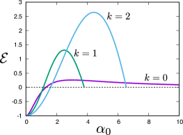
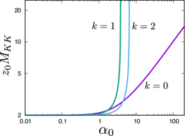
Figure 1: (Left) Energy density as a function of $\alpha_{0}$. (Right) Location of the tip of the AdS soliton $z_{0}$ as a function of $\alpha_{0}$.

In Fig. 2, we show the physical quantities of the resonating AdS soliton. We choose the energy density $\mathcal{E}$ as the horizontal axis. The left edge, $\mathcal{E}=-1$, corresponds to the AdS soliton limit. The other endpoints of the curves correspond to the pure AdS limit, where $\mathcal{E}\to 0$. Because $\mathcal{E}$ takes the maximum value halfway, physical quantities are multivalued in $\mathcal{E}>0$. In particular, two different solutions can be found at $\mathcal{E}=0$: resonating AdS soliton and the pure AdS. As seen in the first panel, the frequency of the resonating AdS soliton satisfies $\omega>kM_{KK}$. We will show in the next subsection that this inequality results in the non-existence of global timelike Killing vectors. In the third panel, we find that the tension $\mathcal{T}$ can take negative values for $k=1,2$. If $\mathcal{T}<0$, negative work is necessary for expanding the radius of the circle with $2\pi/M_{KK}$. In the figure for $\pi_{\chi}$ (last panel), cusps can be observed. Note that $\pi_{\chi}=0$ for $k=0$, which is omitted in the figure. For $k\neq 0$, we checked that the first law of thermodynamics $d\mathcal{E}=\omega/(kM_{KK})d\pi_{\chi}$ is satisfied within numerical errors.

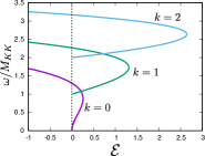
(a) Frequency

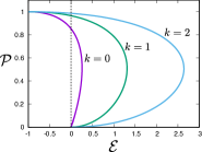
(b) Pressure

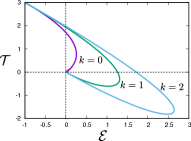
(c) Tension

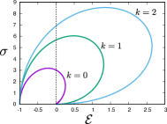
(d) Shear stress

(e) Momentum

Figure 2: Physical quantities of the resonating AdS soliton as a function of the energy density.

4.2 Dynamical spacetime

Does the resonating AdS soliton spacetime have global timelike Killing vectors? A general linear combination of the Killing vectors $\{K_{1},K_{2},\partial_{x},\partial_{y}\}$ can be given by

$$K=c_{1}\left(\partial_{t}+\frac{\omega}{2}\xi_{0}\right)+c_{2}\left(\partial_{\theta}-\frac{k}{2}\xi_{0}\right)\ ,$$ (47)

where

$$\xi_{0}=(x-x_{0})\partial_{y}-(y-y_{0})\partial_{x}\ ,$$ (48)

and $c_{1},\,c_{2},\,x_{0}$ and $y_{0}$ are arbitrary parameters specifying the linear combination. The norm of $K$ is given by

$$K^{2}=g_{\mu\nu}K^{\mu}K^{\nu}=c_{1}^{2}g_{tt}+2c_{1}c_{2}g_{t\theta}+c_{2}^{2}g_{\theta\theta}+\frac{(c_{1}\omega-c_{2}k)^{2}}{4}\xi_{0}^{2}\ ,$$ (49)

where $\xi_{0}^{2}=g_{\mu\nu}\xi_{0}^{\mu}\xi_{0}^{\nu}$. Near the AdS boundary, $\xi_{0}^{2}$ becomes

$$\xi_{0}^{2}\simeq\frac{(x-x_{0})^{2}+(y-y_{0})^{2}}{z^{2}}\ .$$ (50)

Thus $\xi_{0}^{2}\to\infty$ as $x,y\to\infty$. This cannot be compensated by $c_{1}^{2}g_{tt}+2c_{1}c_{2}g_{t\theta}+c_{2}^{2}g_{\theta\theta}$ which does not depend on $x$ and $y$. For this reason, we choose $c_{1}=k$ and $c_{2}=\omega$ to eliminate the term of $\xi_{0}^{2}$ in Eq. (49) and consider a specific combination $K=k\partial_{t}-\omega\partial_{\theta}$. Then, near the AdS boundary, we obtain

$$K^{2}\simeq\frac{\omega^{2}-k^{2}M_{KK}^{2}}{M_{KK}^{2}z^{2}}\ .$$ (51)

Hence $K$ cannot be timelike unless $\omega<kM_{KK}$. However, as shown in Fig. 2(a), we always have $\omega>kM_{KK}$, and therefore $K^{2}>0$. Thus the resonating AdS soliton is a dynamical spacetime.

4.3 Free energy

The renormalized gravitational Lorentzian action is given by Balasubramanian:1999re

$$I_{L}=\frac{1}{16\pi G_{5}}\int_{z\geq\epsilon}d^{5}x\sqrt{-\textrm{det}\,g_{\mu\nu}}\left(R+12\right)\\ -\frac{1}{8\pi G_{5}}\int_{z=\epsilon}d^{4}x\sqrt{-\gamma}K-\frac{3}{8\pi G_{5}}\int_{z=\epsilon}d^{4}x\sqrt{-\gamma}\left(1+\frac{\mathcal{R}}{12}\right)\ ,$$ (52)

where $\gamma_{ij}$ is the induced metric on the $z=\epsilon$ surface, its determinant is denoted by $\gamma=\textrm{det}\,\gamma_{ij}$, and $\mathcal{R}$ is the Ricci scalar with respect to $\gamma_{ij}$. The trace of the extrinsic curvature $K$ is also defined with respect to $\gamma_{ij}$,

$$K=\gamma_{ij}K^{ij}\ ,\qquad K^{ij}=-\frac{1}{2}(\nabla^{i}n^{j}+\nabla^{j}n^{i})\ ,$$ (53)

where $n^{i}$ is the outward pointing unit normal vector at $z=\epsilon$. Note that $R=-20$ from the Einstein equations, and the first term becomes just a volume integral.

For stationary spacetime, the Euclidean on-shell action $I_{E}$ is obtained by replacing $\int dt\to-\int^{1/T}_{0}d\tau$ in the Lorentzian action $I_{L}$, and the free energy is related to the Euclidean action as $\mathcal{F}=TI_{E}$. For general dynamical spacetime, however, we cannot define the Euclidean action and free energy like stationary spacetime. Even though the resonating AdS soliton is a dynamical spacetime, the on-shell Lagrangian is fortunately time-independent. We take advantage of this feature and can define the free energy of the resonating AdS soliton.

For the metric of the resonating AdS soliton (24), we obtain

$$\begin{split}&\sqrt{-\gamma}=\frac{z_{0}\sqrt{\beta_{\infty}}}{2z^{4}}-\frac{\sqrt{\beta_{\infty}}(1-c_{f}-c_{\beta})}{4z_{0}^{3}}+\cdots\ ,\\ &\sqrt{-\gamma}K=-\frac{2z_{0}\sqrt{\beta_{\infty}}}{z^{4}}+\frac{\sqrt{\beta_{\infty}}(1-c_{f}-c_{\beta})}{z_{0}^{3}}+\cdots\ ,\\ &\mathcal{R}=\mathcal{O}(z^{10})\ .\end{split}$$ (54)

Substituting these into Eq.(52) and including the $\mathcal{O}(z^{-4})$ terms into the integrand, we obtain

$$I_{L}=-\frac{z_{0}V_{2}}{2G_{5}}\int dt\left[\int_{0}^{z_{0}}\frac{dz}{z^{5}}\left(\sqrt{\frac{f\beta}{g}}-\sqrt{\beta_{\infty}}\right)-\frac{\sqrt{\beta_{\infty}}(1+c_{f}+c_{\beta})}{8z_{0}^{4}}\right]\ ,$$ (55)

where $V_{2}=\int dxdy$. In this expression, the $z$-integral converges at the AdS boundary $z=0$, and therefore we can set $\epsilon=0$. The Euclidean action $I_{E}$ can be obtained by replacing $\int dt\to-1/T$. Then, the free energy $\mathcal{F}=TI_{E}$ is given by

$$\mathcal{F}=\frac{z_{0}V_{2}}{2G_{5}}\left[\int_{0}^{z_{0}}\frac{dz}{z^{5}}\left(\sqrt{\frac{f\beta}{g}}-\sqrt{\beta_{\infty}}\right)-\frac{\sqrt{\beta_{\infty}}(1+c_{f}+c_{\beta})}{8z_{0}^{4}}\right]\ .$$ (56)

For the undeformed AdS soliton, $f(r)=g(r)=\alpha(r)=\beta(r)=1$ and $h(r)=0$, the free energy of the AdS soliton is given by

$$\mathcal{F}_{\textrm{AdS soliton}}=-\frac{V_{2}}{16G_{5}z_{0}^{3}}=-\frac{V_{2}M_{KK}^{3}}{128G_{5}}\ .$$ (57)

The free energy of the resonating AdS soliton is shown in Fig. 3 for $k=0,1,2$. The normalization is given by the absolute value of the free energy of the AdS soliton. We find that the free energy of the resonating AdS soliton is always bigger than that of the AdS soliton. This behavior has already been observed in the perturbative results Hartnett:2012np . We find that it is the case also in fully nonlinear solutions. The indication of the higher free energy is that the resonating AdS soliton is thermodynamically subdominant in the canonical ensemble. For the dual field theory, this is consistent with the no-go theorem for time crystals as the ground state Watanabe:2014hea .

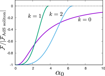
Figure 3: Free energy of the resonating AdS soliton as a function of $\alpha_{0}$.

5 Conclusion

We constructed the resonating AdS soliton as the nonlinear extension of normal modes of the static AdS soliton. We focused on the spin-2 homogeneous perturbation of the AdS soliton, which breaks the isometries (3) to smaller ones (17). In particular, the time translation of the AdS soliton is broken, and a helical isometry given by $K_{1}$ is realized. We introduced the cohomogeneity-1 metric ansatz (24) and obtained the solutions of the resonating AdS soliton numerically. It was shown that the resonating AdS soliton is a non-stationary dynamical spacetime. The pressure and shear stress behave time periodically, while other thermodynamic quantities are time independent.

In Biasi:2019eap , periodic driving by the boundary source of metric has been studied for the four dimensional AdS soliton, and time dependent solutions have been obtained by solving PDEs. In the zero amplitude limit of the driving, they become spontaneously time periodic solutions. The resonating AdS soliton is analogous to them. In the present work, however, by going to five dimensions, we were able to use the cohomogeneity-1 metric ansatz (24) and constructed the time periodic solution without applying boundary driving and dealing with PDEs.

The energy of the resonating AdS soliton is higher than that of the AdS soliton (see Fig. 1). The static AdS soliton has been conjectured to be the minimal energy solution among those with the same boundary topology Horowitz:1998ha ; Constable:1999gb , and the higher energy of the resonating AdS soliton is in accord with this conjecture. The free energy of the resonating AdS soliton is also higher than that of the static AdS soliton as shown in Fig. 3. Hence, the resonating AdS soliton is thermodynamically subdominant.

For the dual field theory, the non-stationary AdS soliton not being the ground state is consistent with the no-go theorem for time crystals as the ground state Watanabe:2014hea . The field theory realization of the time periodic solution dual to the resonating AdS soliton remains unclear, but we are sure it would be an excited state. It might be interpreted as a homogeneous coherent excitation of glueballs in the confined phase of the Yang-Mills theory and characterized by the time dependence in the pressure and shear stress.

In Fig. 2, we observed that the physical quantities are multivalued for a fixed $\mathcal{E}>0$. This behavior typically implies the presence of instability. On the one hand, it would be interesting to look at linear perturbations of the resonating AdS soliton. In global AdS space, cohomogeneity-1 geons are linearly stable in a large portion of parameter space Ishii:2020muv , and the current horizonless solution may share the same property, especially in the branch of small deformation, while the highly deformed branch may have a different behavior and show linear instability instead.

On the other hand, time evolution of the resonating AdS soliton can also be considered directly. At a fixed $\mathcal{E}>0$, a straightforward jump from one of the branches to the other is a possibility, but other dynamics may be involved. Also, the resonating AdS soliton itself is a dynamical spacetime in the first place, and it may develop into a different deformation of the AdS soliton. In Craps:2015upq ; Myers:2017sxr , quenches and time evolution have been studied for the AdS soliton. Similar computations for the resonating AdS soliton will be interesting.

- (1) G. T. Horowitz and R. C. Myers, The AdS / CFT correspondence and a new positive energy conjecture for general relativity, Phys. Rev. D 59 (1998) 026005 [hep-th/9808079].
- (2) N. R. Constable and R. C. Myers, Spin two glueballs, positive energy theorems and the AdS / CFT correspondence, JHEP 10 (1999) 037 [hep-th/9908175].
- (3) G. Galloway, S. Surya and E. Woolgar, A Uniqueness theorem for the AdS soliton, Phys. Rev. Lett. 88 (2002) 101102 [hep-th/0108170].
- (4) G. Galloway, S. Surya and E. Woolgar, On the geometry and mass of static, asymptotically AdS space-times, and the uniqueness of the AdS soliton, Commun. Math. Phys. 241 (2003) 1 [hep-th/0204081].
- (5) E. Woolgar, The rigid Horowitz-Myers conjecture, JHEP 03 (2017) 104 [1602.06197].
- (6) H. Barzegar, P. T. Chruściel, M. Hörzinger, M. Maliborski and L. Nguyen, Remarks on the energy of asymptotically Horowitz-Myers metrics, Phys. Rev. D 101 (2020) 024007 [1907.04019].
- (7) J. M. Maldacena, The Large N limit of superconformal field theories and supergravity, Int. J. Theor. Phys. 38 (1999) 1113 [hep-th/9711200].
- (8) S. Gubser, I. R. Klebanov and A. M. Polyakov, Gauge theory correlators from noncritical string theory, Phys. Lett. B 428 (1998) 105 [hep-th/9802109].
- (9) E. Witten, Anti-de Sitter space and holography, Adv. Theor. Math. Phys. 2 (1998) 253 [hep-th/9802150].
- (10) E. Witten, Anti-de Sitter space, thermal phase transition, and confinement in gauge theories, Adv. Theor. Math. Phys. 2 (1998) 505 [hep-th/9803131].
- (11) S. Hawking and D. N. Page, Thermodynamics of Black Holes in anti-De Sitter Space, Commun. Math. Phys. 87 (1983) 577.
- (12) S. Surya, K. Schleich and D. M. Witt, Phase transitions for flat AdS black holes, Phys. Rev. Lett. 86 (2001) 5231 [hep-th/0101134].
- (13) P. Basu, D. Das and A. Ghosh, Integrability Lost, Phys. Lett. B 699 (2011) 388 [1103.4101].
- (14) T. Ishii, K. Murata and K. Yoshida, Fate of chaotic strings in a confining geometry, Phys. Rev. D 95 (2017) 066019 [1610.05833].
- (15) R. C. Brower, S. D. Mathur and C.-I. Tan, Discrete spectrum of the graviton in the AdS(5) black hole background, Nucl. Phys. B 574 (2000) 219 [hep-th/9908196].
- (16) O. J. Dias, G. T. Horowitz and J. E. Santos, Gravitational Turbulent Instability of Anti-de Sitter Space, Class. Quant. Grav. 29 (2012) 194002 [1109.1825].
- (17) G. T. Horowitz and J. E. Santos, Geons and the Instability of Anti-de Sitter Spacetime, Surveys Diff. Geom. 20 (2015) 321 [1408.5906].
- (18) G. Martinon, G. Fodor, P. Grandclément and P. Forgàcs, Gravitational geons in asymptotically anti-de Sitter spacetimes, Class. Quant. Grav. 34 (2017) 125012 [1701.09100].
- (19) G. Fodor and P. Forgács, Anti–de Sitter geon families, Phys. Rev. D 96 (2017) 084027 [1708.09228].
- (20) O. J. Dias, G. T. Horowitz and J. E. Santos, Black holes with only one Killing field, JHEP 07 (2011) 115 [1105.4167].
- (21) S. L. Liebling and C. Palenzuela, Dynamical Boson Stars, Living Rev. Rel. 20 (2017) 5 [1202.5809].
- (22) M. Maliborski and A. Rostworowski, Time-Periodic Solutions in an Einstein AdS–Massless-Scalar-Field System, Phys. Rev. Lett. 111 (2013) 051102 [1303.3186].
- (23) A. Buchel, S. L. Liebling and L. Lehner, Boson stars in AdS spacetime, Phys. Rev. D 87 (2013) 123006 [1304.4166].
- (24) G. Fodor, P. Forgács and P. Grandclément, Self-gravitating scalar breathers with negative cosmological constant, Phys. Rev. D 92 (2015) 025036 [1503.07746].
- (25) M. W. Choptuik, Ó. J. Dias, J. E. Santos and B. Way, Collapse and Nonlinear Instability of AdS Space with Angular Momentum, Phys. Rev. Lett. 119 (2017) 191104 [1706.06101].
- (26) M. Choptuik, J. E. Santos and B. Way, Charting Islands of Stability with Multioscillators in anti–de Sitter space, Phys. Rev. Lett. 121 (2018) 021103 [1803.02830].
- (27) T. Ishii and K. Murata, Black resonators and geons in AdS5, Class. Quant. Grav. 36 (2019) 125011 [1810.11089].
- (28) T. Ishii and K. Murata, Photonic black resonators and photon stars in AdS5, Class. Quant. Grav. 37 (2020) 075009 [1910.03234].
- (29) G. S. Hartnett and G. T. Horowitz, Geons and Spin-2 Condensates in the AdS Soliton, JHEP 01 (2013) 010 [1210.1606].
- (30) P. Bizon and A. Rostworowski, On weakly turbulent instability of anti-de Sitter space, Phys. Rev. Lett. 107 (2011) 031102 [1104.3702].
- (31) B. Craps, E. J. Lindgren and A. Taliotis, Holographic thermalization in a top-down confining model, JHEP 12 (2015) 116 [1511.00859].
- (32) R. C. Myers, M. Rozali and B. Way, Holographic Quenches in a Confined Phase, J. Phys. A 50 (2017) 494002 [1706.02438].
- (33) S. W. Hawking and H. S. Reall, Charged and rotating AdS black holes and their CFT duals, Phys. Rev. D61 (2000) 024014 [hep-th/9908109].
- (34) H. S. Reall, Higher dimensional black holes and supersymmetry, Phys. Rev. D 68 (2003) 024024 [hep-th/0211290].
- (35) V. Cardoso and O. J. C. Dias, Small Kerr-anti-de Sitter black holes are unstable, Phys. Rev. D70 (2004) 084011 [hep-th/0405006].
- (36) H. K. Kunduri, J. Lucietti and H. S. Reall, Gravitational perturbations of higher dimensional rotating black holes: Tensor perturbations, Phys. Rev. D 74 (2006) 084021 [hep-th/0606076].
- (37) V. Cardoso, O. J. Dias and S. Yoshida, Classical instability of Kerr-AdS black holes and the issue of final state, Phys. Rev. D 74 (2006) 044008 [hep-th/0607162].
- (38) K. Murata, Instabilities of Kerr-AdS(5) x S**5 Spacetime, Prog. Theor. Phys. 121 (2009) 1099 [0812.0718].
- (39) H. Kodama, R. Konoplya and A. Zhidenko, Gravitational instability of simply rotating AdS black holes in higher dimensions, Phys. Rev. D 79 (2009) 044003 [0812.0445].
- (40) Ó. J. Dias and J. E. Santos, Boundary Conditions for Kerr-AdS Perturbations, JHEP 10 (2013) 156 [1302.1580].
- (41) V. Cardoso, Ó. J. Dias, G. S. Hartnett, L. Lehner and J. E. Santos, Holographic thermalization, quasinormal modes and superradiance in Kerr-AdS, JHEP 04 (2014) 183 [1312.5323].
- (42) Ó. J. Dias, J. E. Santos and B. Way, Black holes with a single Killing vector field: black resonators, JHEP 12 (2015) 171 [1505.04793].
- (43) B. E. Niehoff, J. E. Santos and B. Way, Towards a violation of cosmic censorship, Class. Quant. Grav. 33 (2016) 185012 [1510.00709].
- (44) S. R. Green, S. Hollands, A. Ishibashi and R. M. Wald, Superradiant instabilities of asymptotically anti-de Sitter black holes, Class. Quant. Grav. 33 (2016) 125022 [1512.02644].
- (45) T. Ishii, K. Murata, J. E. Santos and B. Way, Superradiant instability of black resonators and geons, 2005.01201.
- (46) P. M. Chesler and D. A. Lowe, Nonlinear Evolution of the AdS4 Superradiant Instability, Phys. Rev. Lett. 122 (2019) 181101 [1801.09711].
- (47) W.-J. Li, Y. Tian and H.-b. Zhang, Periodically Driven Holographic Superconductor, JHEP 07 (2013) 030 [1305.1600].
- (48) M. Natsuume and T. Okamura, The enhanced holographic superconductor: is it possible?, JHEP 08 (2013) 139 [1307.6875].
- (49) R. Auzzi, S. Elitzur, S. B. Gudnason and E. Rabinovici, On periodically driven AdS/CFT, JHEP 11 (2013) 016 [1308.2132].
- (50) M. Rangamani, M. Rozali and A. Wong, Driven Holographic CFTs, JHEP 04 (2015) 093 [1502.05726].
- (51) K. Hashimoto, S. Kinoshita, K. Murata and T. Oka, Holographic Floquet states I: a strongly coupled Weyl semimetal, JHEP 05 (2017) 127 [1611.03702].
- (52) S. Kinoshita, K. Murata and T. Oka, Holographic Floquet states II: Floquet condensation of vector mesons in nonequilibrium phase diagram, JHEP 06 (2018) 096 [1712.06786].
- (53) A. Biasi, P. Carracedo, J. Mas, D. Musso and A. Serantes, Floquet Scalar Dynamics in Global AdS, JHEP 04 (2018) 137 [1712.07637].
- (54) T. Ishii and K. Murata, Floquet superconductor in holography, Phys. Rev. D 98 (2018) 126005 [1804.06785].
- (55) A. Biasi, J. Mas and A. Serantes, Gravitational wave driving of a gapped holographic system, JHEP 05 (2019) 161 [1903.05618].
- (56) C. Csaki, H. Ooguri, Y. Oz and J. Terning, Glueball mass spectrum from supergravity, JHEP 01 (1999) 017 [hep-th/9806021].
- (57) R. de Mello Koch, A. Jevicki, M. Mihailescu and J. P. Nunes, Evaluation of glueball masses from supergravity, Phys. Rev. D 58 (1998) 105009 [hep-th/9806125].
- (58) M. Zyskin, A Note on the glueball mass spectrum, Phys. Lett. B 439 (1998) 373 [hep-th/9806128].
- (59) A. Ashtekar and S. Das, Asymptotically Anti-de Sitter space-times: Conserved quantities, Class. Quant. Grav. 17 (2000) L17 [hep-th/9911230].
- (60) S. Kinoshita, S. Mukohyama, S. Nakamura and K.-y. Oda, A Holographic Dual of Bjorken Flow, Prog. Theor. Phys. 121 (2009) 121 [0807.3797].
- (61) V. Balasubramanian and P. Kraus, A Stress tensor for Anti-de Sitter gravity, Commun. Math. Phys. 208 (1999) 413 [hep-th/9902121].
- (62) S. de Haro, S. N. Solodukhin and K. Skenderis, Holographic reconstruction of space-time and renormalization in the AdS / CFT correspondence, Commun. Math. Phys. 217 (2001) 595 [hep-th/0002230].
- (63) M. Bianchi, D. Z. Freedman and K. Skenderis, Holographic renormalization, Nucl. Phys. B 631 (2002) 159 [hep-th/0112119].
- (64) H. Watanabe and M. Oshikawa, Absence of Quantum Time Crystals, Phys. Rev. Lett. 114 (2015) 251603 [1410.2143].