Quantum annealing speedup of embedded problems via suppression of Griffiths singularities

Abstract

Optimal parameter setting for applications problems embedded into hardware graphs is key to practical quantum annealers (QA). Embedding chains typically crop up as harmful Griffiths phases, but can be used as a resource as we show here: to balance out singularities in the logical problem changing its universality class. Smart choice of embedding parameters reduces annealing times for random Ising chain from $O(\exp[c\sqrt{N}])$ to $O(N^{2})$. Dramatic reduction in time-to-solution for QA is confirmed by numerics, for which we developed a custom integrator to overcome convergence issues.

Implementation of quantum annealing Kadowaki and Nishimori (1998); Farhi et al. ; *farhi2001quantum; Das and Chakrabarti (2008); Albash and Lidar (2018) for optimization problems expressed as unconstrained quadratic forms of binary variables requires embedding Choi (2008); *choi2011minor; Hilton et al. (2019) the connectivity topology of the problem into that of the underlying hardware. This typically means representing logical qubits in terms of clusters of physical qubits designed to be ferromagnetically aligned at the completion of the annealing cycle. Performance suffers as a result: Not only does it lead to a decreased utilization of qubits, but since the effective two-level system for strongly coupled qubits is endowed with slower dynamics, it becomes more susceptible to harmful non-adiabatic excitations. Judicious choice of embedding parameters to minimize these effects has large practical utility and remains an active area of research. Most of the earlier work studied optimal parameter setting empirically by running experiments on D-Wave annealers as well as formulating educated guesses based on classical and quantum spectrum and intuition from the theory of phase transitions King and McGeoch ; Venturelli et al. (2015); Fang and Warburton ; Harris et al. (2018).

The adiabatic quantum computing protocol obtains a solution by evolving, in a finite time interval $[0;T]$, a time-dependent Hamiltonian that interpolates between a “driver” term with easily obtainable ground state and the “classical” Hamiltonian which is diagonal in Z-basis and encodes the cost of underlying quadratic unconstrained binary optimization (QUBO) problem:

$$H(t)=-\bigl{(}1-\tfrac{t}{T}\bigr{)}\sum_{i}X_{i}-\tfrac{t}{T}\Biggl{(}\sum_{\langle ik\rangle}J_{ik}Z_{i}Z_{k}+\sum_{i}h_{i}Z_{i}\Biggr{)}.$$ (1)

The time-dependent Hamiltonian describes the annealing of Ising spins on a graph as the external uniform magnetic field $\Gamma=\frac{1-s}{s}$ (where $s=\frac{t}{T}$) is applied in the transverse direction and decreases to zero. Adiabatic theorem ensures that for sufficiently large $T$ the system remains close to its instantaneous ground state until the driver term that causes bit flips vanishes at the end of the annealing algorithm. Very recently it has been shown theoretically that even a simple driver such as the transverse field could in principle achieve a superpolynomial speedup against classical computing Hastings .

Known empirical evidence suggests that high probability of success is best achieved by performing many independent runs over optimally chosen annealing cycle time $T$. The probability of error $\epsilon=(1-p_{0})^{L}$ can be made arbitrarily small using large number of repeats $L$ (here $p_{0}$ is the success probability of a single run). The total computation time $\mathcal{T}=TL$ is expressed in terms of unambiguous time-to-solution metric $\mathcal{T}=\tau\log(1/\epsilon)$ that we adopt here:

$$\tau=\min_{T}\frac{T}{\bigl{|}\log[1-p_{0}(T)]\bigr{|}}.$$ (2)

Although we restrict ourselves to a linear schedule with driver term and classical term prefactors $A(s)=1-s$ and $B(s)=s$ for the sake of simplicity, singularities at $s=0$ and $s=1$ dictate the scaling of $p_{0}(T)$ only for very large $T$. Using a sweet-spot value of $T$ ensures that our results remain qualitatively robust for a general non-linear interpolating schedule typically constrained by a specific hardware implementation.

The illustrative example that is the subject this letter is a simple model: a one-dimensional chain of ferromagnetically coupled Ising spins (qubits) with random interactions,

$$H(s)=(1-s)H_{D}+sH_{C},\text{ with }H_{C}=-\sum_{i=1}^{N}J_{i}Z_{i-1}Z_{i}$$ (3)

(in zero longitudinal field, $h_{i}=0$) with the usual choice of a driver term that represents a transverse field, $H_{D}=-\sum_{i}X_{i}$. The annealing bottleneck for this problem is related to a quantum critical point separating paramagnetic and ferromagnetic phases. Without randomness, i.e. if all $J_{i}=1$, the energy gap that separates the ground state from excited states within the symmetric subspace is minimized at $s_{c}=1/2$ ($\Gamma_{c}=1$). Notice that we disregard one half of the states (including the first excited state) that are never populated due to $H(t)$ preserving a global symmetry $\left[U=\exp\frac{\pi\mathrm{i}}{2}\sum_{i}X_{i}\right]$ which flips all bits: $Z_{i}\rightarrow-Z_{i}$. The critical exponents that can be obtained either from an analytic solution via fermionization or from the renormalization group (RG) analysis predict that correlation length $\xi\sim|s-s_{c}|^{-1}$ and the gap in the paramagnetic phase $\Delta E\sim(s_{c}-s)$. This suggests a cutoff value of the gap $\Delta E_{c}\sim 1/N$ as the correlation length $\xi$ reaches the system size $N$, and, therefore, polynomial scaling for TTS metric $\tau\sim(\Delta E_{c}\cdot\Delta s_{c})^{-1}\sim N^{2}$. This scaling is intimately related to Kibble-Zureck mechanism of quench dynamics across the phase transition Zurek et al. (2005); Dziarmaga (2005).

By contrast, if couplings $J_{i}$ are randomly distributed and are not correlated, the RG flow is toward an infinite-randomness fixed point (IRFP) with the gap $\Delta E\sim\exp(-c\sqrt{\xi})$, i.e. the minimum gap scales with $N$ as a stretched exponential Fisher (1992); *fisher1995critical. This anomalous scaling is due to the presence of Griffiths-McCoy singularities Griffiths (1969); *mccoy1969incompleteness as different parts of the system are unable to reach criticality simultaneously as a result of strong disorder fluctuations.

To illustrate, consider uniform distribution of the couplings $J_{k}\in[0;1]$. The critical value of the transverse field is the geometric mean, i.e. the gap to the 2${}^{\text{nd}}$ excited state is minimized at $\Gamma_{c}=1/\mathrm{e}$ (corresponding to $s_{c}=(1+1/\mathrm{e})^{-1}\approx 0.731$). If the chain is cut in two equal parts at criticality, the subchains will have $\Gamma_{c}^{1,2}=\Gamma_{c}\pm\Delta\Gamma_{c}$ where $\Delta\Gamma_{c}\sim 1/\sqrt{N}$ by central limit theorem. One part will be ferromagnetically ordered with gap $\Delta E_{c}\sim\exp{(-cN\Delta\Gamma_{c})}$. This only demonstrates stretched exponential scaling for the gap to the first excited state, which is not relevant to the transverse field parity-conserving dynamics. However, it is expected that entire low-energy spectrum has the same universal scaling form (see Appendix A for a rigorous discussion). In practice, the asymptotic scaling will not set in until $N$ becomes moderately large, whereas scaling for small system sizes may be indistinguishable from that of a non-disordered chain.

Embedding using block spins.

For this study we set out to explore strategies for setting parameters for embeddings in coherent quantum annealers, which replace logical qubits with blocks of $M$ ferromagnetically coupled physical qubits. This is done primarily to increase the connectivity of qubit interaction graph [to $M(c-2)+2$, where $c$ is the degree of connectivity graph of physical hardware]. The extreme example achieves all-to-all connectivity at the cost of quadratic reduction of the number of logical qubits [to $O\bigl{(}\sqrt{N}\bigr{)}$] as seen in Refs. Choi, 2008, 2011. Another important application is extending the range of Ising couplings, which is more relevant for the present study of a linear chain ($c=2$). Lastly, using block spins has been suggested as a form of error-correction Pudenz et al. (2014); *pudenz2015quantum; Vinci et al. (2015); Matsuura et al. (2017).

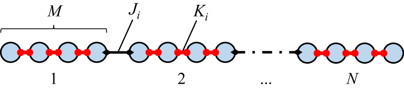
Figure 1: A simple model of embedding. A logical problem corresponds to 1D spin chain with ferromagnetic couplings $J_{i}$. Embedded problem replaces each logical spin with a block (chain) of $M$ physical spins having intra-chain coupling $K_{i}$.

As we introduce $M$ ancillary spins for each logical variable (see Fig. 1), the classical Hamiltonian reads

$$H_{C}=-\sum_{k=1}^{NM-1}\tilde{J}_{k}Z_{k-1}Z_{k},$$ (4)

$$\text{with}\quad\tilde{J}_{Mi}=J_{i},\quad 1\leqslant i\leqslant N-1,$$

$$\text{and}\quad\tilde{J}_{Mi+1}=\cdots=J_{Mi+(M-1)}=K_{i},\quad 0\leqslant i\leqslant N-1.$$

For simplicity, the ferromagnetic couplings $K_{i}$ within a subchain are taken to be uniform but we allow variations from one logical qubit to another. To ensure that these ferromagnetic links are never broken in any local minimum we insist that

$$\min_{0\leqslant i\leqslant N-1}K_{i}>\max_{1\leqslant i\leqslant N-1}J_{i}.$$ (5)

Since the model retains its 1D character, existing analytical techniques are still applicable and numerical studies can explore a regime where annealing becomes intractable for large $N$.

Specifically, we observe that for sufficiently small values of the transverse field $\tilde{\Gamma}<\min_{i}K_{i}$ we may perform the real-space renormalization procedure due to D. S. Fisher Fisher (1992); *fisher1995critical. Each subchain now behaves as a spin subjected to a transverse field with the renormalized value

$$\Gamma_{i}=\frac{\tilde{\Gamma}^{M}}{\prod_{k=Mi+1}^{Mi+M-1}\tilde{J}_{k}}=\frac{\tilde{\Gamma}^{M}}{K_{i}^{M-1}}.$$ (6)

(In a reversal of notation used in Ref. Fisher, 1992; *fisher1995critical, we write $\tilde{\Gamma}=\frac{s}{1-s}$ to represent the bare value of the transverse field and reserve non-accented letters $\Gamma_{i}$ to denote the renormalized fields.) The effective model is still an Ising chain

$$H=s\left[-\sum_{i=1}^{N-1}J_{i}Z_{i-1}Z_{i}-\sum_{i=0}^{N-1}\Gamma_{i}X_{i}\right],$$ (7)

albeit with the local transverse field that can potentially have spatial variations.

The embedding procedure thus unlocks an important resource since many existing implementations either lack such local control entirely or have limited dynamic range. It allows us to restore the polynomial scaling of annealing complexity, balancing out disorder fluctuations to synchronize the phase transition across entire chain. We make the following ansatz for embedding parameters

$$K_{i}=C(J_{i}J_{i+1})^{-\frac{1}{2(M-1)}}\quad(i=1,\ldots,N-2)$$ (8)

for some rescaling constant $C.$ At the edges we can use, e.g., $K_{0}=CJ_{1}^{-1/(M+1)}$ and $K_{N-1}=CJ_{N-1}^{-1/(M+1)}$.

With this choice, renormalized local fields in the bulk become $\Gamma_{i}=\frac{\tilde{\Gamma}^{M}}{C^{M-1}}\sqrt{J_{i}J_{i+1}}$ so that fluctuations of the value of the critical field $\Delta\tilde{\Gamma}_{c}$ for large subchains now scale as $1/N$.

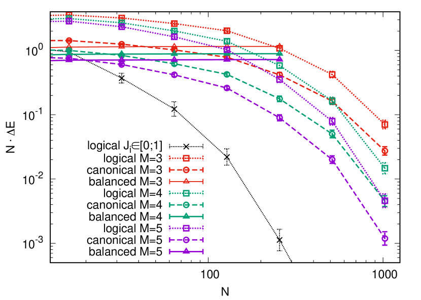
Figure 2: Normalized median value of the minimum gap ($N\cdot\Delta E_{c}$) vs problem size. Black solid line corresponds to the logical problem with strong disorder ($J_{i}\in[0;1]$). Results for embedded variants with $M=3,4,5$ are shown with solid and dashed color lines for, respectively, the balanced choice of embedding parameters given by scaled-down form of Eq. (8) and the canonical choice $K_{i}=1$. The disorder distributions used for embedded variants are those uniform in the interval $[1/M;1]$. For reference, the median values of the minimum gap of the logical problem for these weaker disorder distributions are also shown using dotted color lines.

In Fig. 2 we compare the median minimum gap for different parameter setting prescriptions, showing that the balanced choice in Eq. (8) recovers a polynomial gap. It is imperative to discuss how the parameters of our numerical study were chosen. The black solid line plots the estimate of the median value (taken over disorder distribution) of the minimum gap for strong disorder: $J_{i}$ are taken to be uniformly distributed in the interval [0;1]. The data clearly cannot be fit by any power law (which would have been a straight line on a log-log plot).

It is evident from Eq. (8) that allowing arbitrarily small values of $J_{i}$ would in turn lead to arbitrarily large values of $K_{i}$. Moreover, small values of $J_{\text{min}}$ are not expected to appear naturally for Ising representations of practical problems Lucas (2014) and would make the problem particularly prone to misspecification errors in hardware annealers.

To mitigate this problem, we choose $J_{i}\in[1/M;1]$, where $M$ is the number of spins in a block. Fig. 2 uses colored dotted line to plot gaps of the logical problem for such disorder distributions. Dashed lines show the gaps for an embedded problem with a canonical choice of embedding parameters ($K_{i}=1$). Balanced choice of embedding parameters from Eq. (8) with $C=1$ would have yielded values $K_{i}$ in a range $[1;M^{1/(M-1)}]$. Current practice for existing hardware implementations of quantum annealing is to use largest possible values of couplings $J_{i}$ in order to minimize misspecification error, hence it is natural to assume that $J=1$ already represents the maximum programmable value. In order to accommodate the balanced parameter setting, all ferromagnetic couplings must be scaled down by a factor of $M^{1/(M-1)}$, i.e. $J_{i}\in[M^{-M/(M-1)};M^{-1/(M-1)}]$ and $C=M^{-M/(M-1)^{2}}$. This rescaling step had been made for the data plotted in Fig. 2 using solid colored lines. The motivation for this peculiar choice of disorder distribution is that it maximizes the range $J_{\text{max}}-J_{\text{min}}$ of inter-chain couplings after the rescaling.

Rescaling of couplings parameters downward handicaps quantum annealing performance. Using rescaled $J^{\prime}=\lambda J$ we can show that $\Delta E_{c}^{\prime}\cdot\Delta s_{c}^{\prime}=(\lambda^{2}s_{c}/s^{\prime}_{c})\Delta E_{c}\cdot\Delta s_{c}$. The scaling factor can be rewritten as $(1-s_{c})\lambda^{3}+s_{c}\lambda^{2}$, which is less than unity if $\lambda<1$. Numerical data for the gap is consistent with this qualitative behavior. More rigorous analysis of the low-energy spectrum along the lines described in Appendix A also predicts that the gap for canonical embedding is smaller than that of the logical problem with the same disorder by $O(M)$ factor, also in agreement with the numerical data.

We encountered a problem specific to instances using balanced embedding, likely due to a quirk in its spectrum: numerical diagonalization could only performed for a smaller range of $N$ as the limits of machine precision were reached. It may be possible to overcome this obstacle using multiprecision arithmetic to find the roots of characteristic polynomial for the tridiagonal matrix. Fortunately, the median gap fits polynomial scaling perfectly (straight line on a log-log plot), which gives us sufficient confidence to extrapolate the data for large $N$.

Time-to-solution analysis.

The one-dimensional Ising chain is the simplest example of an integrable quantum model. A rotation ($X_{i}\rightarrow-Z_{i}$, $Z_{i}\rightarrow X_{i}$) followed by a Jordan-Wigner transformation expresses the Hamiltonian as a quadratic form in fermionic operators. The solution of time-dependent Bogolyubov-de Gennes (BdG) equations is used to write these operators in Heisenberg representation (which is a linear combination of Schrödinger operators since $H$ is quadratic Dziarmaga (2006); Caneva et al. (2007)). For instance, using Majorana representation (see e.g. Ref. Fradkin, 2013) ($\chi_{2i}=X_{i}\prod_{k=0}^{i-1}Z_{k}$ and $\chi_{2i+1}=Y_{i}\prod_{k=0}^{i-1}Z_{k}$) we can write

$$\boldsymbol{\chi}(t)=\mathbf{S}(t)\boldsymbol{\chi}(0),\quad\frac{\mathrm{d}\mathbf{S}}{\mathrm{d}t}=2\mathbf{M}\mathbf{S}.$$ (9)

Here $\mathbf{S}$ is special orthogonal $2n\times 2n$ matrix, whereas $\mathbf{M}$ is skew-symmetric and also happens to be tridiagonal with the elements on the upper diagonal $M_{2i,2i+1}=1-s$ and $M_{2i-1,2i}=sJ_{i-1}$. This special structure further aids numerics; on top of logarithmic reduction in complexity afforded by the free-fermion mapping.

Eigenvalues of $\mathbf{M}$ (e.g. for ordering $\lambda_{2k}=+\mathrm{i}\epsilon_{k}$, $\lambda_{2k+1}=-\mathrm{i}\epsilon_{k}$ with $0<\epsilon_{0}<\cdots<\epsilon_{N-1}$) completely determine the spectrum of the instantaneous Hamiltonian $H(t)$ as a sum of single-particle excitations: $E_{\{n_{k}\}}=2\sum_{k}n_{k}\epsilon_{k}$ where $n_{k}\in\{0,1\}$. Specifically, the gap between the ground state and the second excited state (which is second lowest in energy among those in the symmetric subspace) is $\Delta E=2(\epsilon_{1}+\epsilon_{2})$. This value enters the adiabatic condition used to estimate the runtime (see Appendix A).

To better quantify the performance we concentrate on a TTS metric of Eq. (2). The probability to find the system in its ground state at the end of the annealing cycle at $t=T$ is

$$p_{0}=\biggl{\langle}\prod_{k}(b_{k}b_{k}^{\dagger})\biggr{\rangle},$$ (10)

where $b_{k}$ and $b_{k}^{\dagger}$ are fermionic quasiparticle operators in Dirac representation that diagonalize the final classical Hamiltonian $H_{C}$. Expectation value can be computed at time $t=0$ provided that Heisenberg representation for $b_{k}(t)$ and $b_{k}^{\dagger}(t)$ is used. The initial state satisfies $a_{i}|0\rangle=0$ where $a_{i}$ and $a_{i}^{\dagger}$ are the Dirac fermion operators that diagonalize the transverse field Hamiltonian $H_{D}$.

Since the Hamiltonian is quadratic, the expectation value (10) is computed by performing the sum over all possible pairings and can be expressed as

$$p_{0}=\sqrt{\det\tfrac{1}{2}(\mathbf{S}\mathbf{A}\mathbf{S}^{T}+\mathbf{B})}$$ (11)

where the only non-zero elements of $\mathbf{A}$, $\mathbf{B}$ are $A_{2k,2k+1}=B_{2k-1,2k}=B_{0,2N-1}=1$ and $A_{2k+1,2k}=B_{2k,2k-1}=B_{2N-1,0}=-1$ (see Appendix B).

Numerical results.

Investigating the complexity using the TTS metric is somewhat challenging numerically. It entails integrating systems of differential equations of more than $10^{4}$ variables for multiple choices of annealing times (in excess of $10^{7}$ in dimensionless units). Numerical error accumulates proportionally to the evolution time, and is further amplified when we evaluate the determinant (11). After multiple tests, we implemented an integrator based on Cayley transform and Magnus expansion Blanes et al. (2000); *blanes2002high up to 8th order. However, we use Padé approximation of the exponential to obtain a straightforward mapping to Cayley transform and exploit the tridiagonal structure of matrix $\mathbf{M}$ to attain best performance. Compared with traditional Runge-Kutta approaches used for these types of problems Mbeng et al. (2019), our method maintains orthogonality of $\mathbf{S}$ at all update steps which significantly improves stability for long integration times (see Appendix C). For a given timestep our implementation outperforms comparable methods such as Dormand-Prince algorithms that are the method of choice in celestial mechanics Dormand and Prince (1980), but also maintains excellent precision for large step sizes $\Delta t$.

Note that since optimal annealing time in Eq. (2) cannot be known in advance, it seems unfair to perform optimization of for each individual instance. We use ensemble-wide $T_{\text{opt}}(N)$, which is determined through minimization, as a function of annealing time, of the median TTS, from a sample of random instances of the same size. This choice is similar to the practice of benchmarking of application problems.

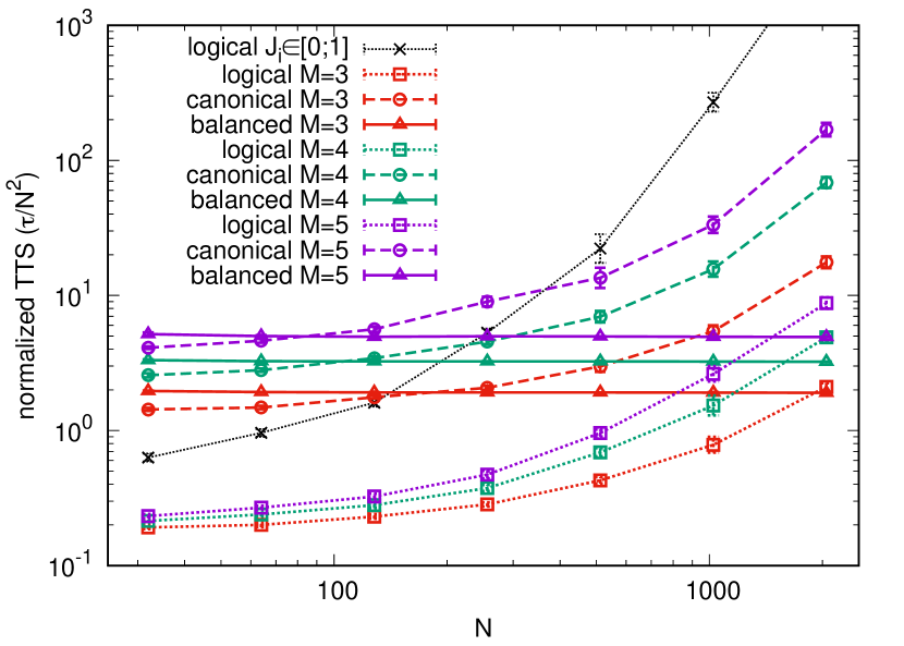
Figure 3: Normalized median time-to-solution (divided by $N^{2}$) as a function of problem size. Block solid line plots TTS for a logical instance with strong disorder for $J\in[0;1]$. Dotted color lines represent logical instances for a disorder in the interval $[1/M;1]$ for $M=3,4,5$. TTS for embedded variants using the same disorder distribution for logical couplings using the canonical and balanced choice of parameters are plotted using dashed and solid color lines, respectively. Errorbars represent the uncertainty of estimating the median using a small sample size of instances and optimization over annealing time.

We plot the median time-to-solution for random instances of increasing size in Fig. 3. As before, colored dotted lines refer to logical problem with $J_{i}\in[1/M;1]$, dashed lines correspond to canonical embedding parameters and solid lines present results for balanced embedding parameters. Finally, black solid line refers to a logical problem with strong disorder $J_{i}\in[0;1]$, where non-polynomial behavior is most pronounced. We observe that for the largest sizes balanced embedding clearly outperforms the canonical one ($K_{i}=1$).

Conclusions

We have investigated quantum annealing of embeddings of a simple problem, where logical qubits were replaced by ferromagnetic chains of Ising spins. A novel ansatz for a balanced choice of coupling parameters based on renormalization group intuition results in an exponential improvement in annealing times. This is corroborated numerically, using time-to-solution metric of complexity. For large sizes the balanced choice significantly outperforms both canonical parameter setting and the quantum annealing of the logical problem using the same distribution of disorder (but with no embedding).

The protocol proposed in this letter succeeds because embedding parameters are set in such a fashion that spatially separate regions achieve criticality simultaneously. A situation were multiple domains oriented in random directions are created is thus avoided. Remarkably, this can be accomplished without local control of the transverse field. Complementary approaches described in literature rely on “growing” the domain and require significant modifications to quantum annealing protocol using time-dependent local control of the transverse field Rams et al. (2016).

An important venue of research is the generalization of this idea to higher-dimensional problems. Dearth of exactly solvable models suggests using approximate methods to find embedding parameters that achieve synchronization of local phase transitions. We expect to be able to suppress Griffiths singularities relieving the phase transition bottleneck of annealing complexity. However, Ising models in higher dimensions exhibit frustration, which dominates complexity for very large instances Knysh (2016) (crafted problems in 1D can also exhibit frustration bottleneck Roberts et al. (2020)). We are cautiously optimistic that this general technique can be useful for intermediate-range problems that could be implemented in highly coherent quantum annealers Novikov et al. (2018). Another research direction is the extension of this work to open systems where the annealing dynamics is incoherent, driven by coupling with an external reservoir Smelyanskiy et al. (2017); Mishra et al. (2018). This would open up the opportunity of testing the balanced embedding approach on D-Wave machines as well Bando et al. .

Appendix A Eigenspectrum

Diagonalization of one-dimensional Ising model is performed using Jordan-Wigner transformation. The Hamiltonian reads in spin representation as

$$H=-\sum_{i=1}^{N-1}J_{i}X_{i-1}X_{i}+\Gamma\sum_{i=0}^{N-1}Z_{i},$$ (12)

where we rotated the basis around $y$-axis by $\pi/2$. We introduce $2N$ Majorana fermions defined via

$$\chi_{2i}=X_{i}\prod_{k=0}^{i-1}Z_{k},\qquad\chi_{2i+1}=Y_{i}\prod_{k=0}^{i-1}Z_{k},$$ (13)

and obeying anti-commutation relations $\{\chi_{i},\chi_{j}\}=2\delta_{ij}$ as can be straightforwardly verified. In terms of these, the Ising Hamiltonian can be rewritten as

$$H=-\mathrm{i}\sum_{i=1}^{N-1}J_{i}\chi_{2i-1}\chi_{2i}+\mathrm{i}\Gamma\sum_{i=0}^{N-1}\chi_{2i}\chi_{2i+1}.$$ (14)

The Hamiltonian can be equivalently represented in terms of Dirac quasiparticles

$$H=\sum_{\nu}\epsilon_{\nu}(\gamma_{\nu}^{{\dagger}}\gamma_{\nu}-\gamma_{\nu}^{{\dagger}}\gamma_{\nu}).$$ (15)

From this representation one obtains all $2^{N}$ energy levels:

$$E_{\mathbf{n}}=E_{0}+2\sum_{\nu}n_{\nu}\epsilon_{\nu},\text{ where $n_{\nu}\in\{0,1\}$ are the occupation numbers and }E_{0}=-\sum_{\nu}\epsilon_{\nu}.$$ (16)

Using identities

$$[\gamma_{\mu},H]=2\epsilon_{\mu}\gamma_{\mu}\qquad\text{and}\qquad[\gamma_{\mu}^{{\dagger}},H]=-2\epsilon_{\mu}\gamma_{\mu}^{{\dagger}}$$ (17)

one obtains the single-fermion excitation energies and creation/annihilation operators from the spectrum of the tridiagonal matrix

$$\mathbf{M}=\left(\begin{array}[]{cccccccc}0&\Gamma&&&&&&\\ -\Gamma&0&J_{1}&&&&&\\ &-J_{1}&0&\Gamma&&&&\\ &&-\Gamma&0&J_{2}&&&\\ &&&-J_{2}&\ddots&\ddots&&\\ &&&&\ddots&\ddots&J_{N-1}&\\ &&&&&-J_{N-1}&0&\Gamma\\ &&&&&&-\Gamma&0\end{array}\right)$$ (18)

that appears Majorana representation of Eq. (14); that is $H=\frac{1}{2}\mathrm{i}\boldsymbol{\chi}^{T}\mathbf{M}\boldsymbol{\chi}$ where $\boldsymbol{\chi}$ is a column vector of Majorana fermions $\chi_{0},\chi_{1},\ldots,\chi_{2N-1}$.

To study the behavior of the gap we write the characteristic equation:

$$\det(\lambda+\mathbf{M}^{2})=0,\quad\mathbf{M}^{2}=-\left(\begin{array}[]{cccccccc}\Gamma^{2}&-\Gamma J_{1}&&&&&&\\ -\Gamma J_{1}&\Gamma^{2}+J_{1}^{2}&\ddots&&&&&\\ &\ddots&\ddots&-\Gamma J_{N-1}&&&&\\ &&-\Gamma J_{N-1}&\Gamma^{2}+J_{N-1}^{2}&&&&\\ &&&&\Gamma^{2}+J_{1}^{2}&-\Gamma J_{1}&&\\ &&&&-\Gamma J_{1}&\ddots&\ddots&\\ &&&&&\ddots&\Gamma^{2}+J_{N-1}^{2}&-\Gamma J_{N-1}\\ &&&&&&-\Gamma J_{N-1}&\Gamma^{2}\end{array}\right).$$ (19)

Above we rearranged the rows and columns of $\mathbf{M}^{2}$ (by grouping even-numbered and odd-numbered) in block-diagonal form. It is straightforward to verify that both blocks yield the same characteristic equation (the terms can be evaluated by computing minors via induction over $N$):

$$\Gamma^{2N}-\lambda\Gamma^{2(N-1)}\sum_{0<k_{1}<k_{2}<N}\frac{\prod_{i=k_{1}}^{k_{2}-1}J_{i}^{2}}{\Gamma^{2(k_{2}-k_{1})}}+\Gamma^{2(N-2)}\lambda^{2}\sum_{0<k_{1}<k_{2}<k_{3}<k_{4}<N}\frac{\prod_{i=k_{1}}^{k_{2}-1}J_{i}^{2}}{\Gamma^{2(k_{2}-k_{1})}}\cdot\frac{\prod_{i=k_{3}}^{k_{4}-1}J_{i}^{2}}{\Gamma^{2(k_{4}-k_{3})}}+\cdots=0.$$ (20)

Indeed, the roots of characteristic equation should be doubly degenerate corresponding to the pairs of eigenvalues $\pm\mathrm{i}\epsilon_{k}$ of matrix $\mathbf{M}$: $\lambda_{k}=\epsilon_{k}^{2}$.

In the region of interest of the disordered problem we expect that $\epsilon_{0}\ll\epsilon_{1}\ll\epsilon_{2}\ll\cdots$ and so on. With this in mind, it suffices to retain terms up to $\lambda^{2}$ to estimate the gap to the second excited state: we approximate $\epsilon_{0}$ and $\epsilon_{1}$ by solutions to a quadratic equation (20). To illustrate this in more detail, Fig. 4 below presents plots of a function (defined for integer $1\leqslant k\leqslant N$)

$$W(k)=\sum_{i=1}^{k-1}\ln J_{i}-k\ln\Gamma$$ (21)

for three different values of $\Gamma$. On large scales $W(k)$ describes a Wiener process (Brownian motion) so that it typically scales as $O\left(\sqrt{N}\right)$. The partial products inside the sums in Eq. (20) may be expressed as $\mathrm{e}^{2[W(k_{2})-W(k_{1})]}$ for a term linear in $\lambda$ or $\mathrm{e}^{2[W(k_{4})-W(k_{3})+W(k_{2})-W(k_{1})]}$ for a term quadratic in $\lambda$. Large exponent ensures that the sums are dominated by just a few terms. Using $W_{1}$, $W_{2}$, $W_{3}$, and $W_{4}$ do denote the extremal values as depicted in Fig. 4 we can write Vieta’s formulae:

$$\frac{1}{\lambda_{0}\lambda_{1}}\sim\mathrm{e}^{2(W_{4}-W_{3}+W_{2}-W_{1})},\qquad\frac{1}{\lambda_{0}}+\frac{1}{\lambda_{1}}\sim\begin{cases}\mathrm{e}^{2(W_{4}-W_{1})}&\text{for }\Gamma<\Gamma_{\ast},\\ \mathrm{e}^{2(W_{2}-W_{1})}&\text{for }\Gamma>\Gamma_{\ast},\end{cases}$$ (22)

where $\Gamma_{\ast}$ has been chose so that $W_{2}\approx W_{4}$. From this we conclude that

$$\epsilon_{0}\sim\mathrm{e}^{-(W_{4}-W_{1})}\quad \text{and}\quad\epsilon_{1}\sim\mathrm{e}^{-(W_{2}-W_{3})} (\Gamma<\Gamma_{\ast}),$$ (23)

$$\epsilon_{0}\sim\mathrm{e}^{-(W_{2}-W_{1})}\quad \text{and}\quad\epsilon_{1}\sim\mathrm{e}^{-(W_{4}-W_{3})} (\Gamma>\Gamma_{\ast}).$$ (24)

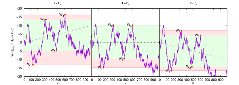
Figure 4: Blue solid line shows realization of random process described by Eq. 21. Black dotted line, $-k(\ln\Gamma-\ln\Gamma_{\ast})$, serves as visual guide to describe vertical shear as $\Gamma$ is varied. From left to right, subplots depicts scenarios $\Gamma<\Gamma_{\ast}$, $\Gamma=\Gamma_{\ast}$, and $\Gamma>\Gamma_{\ast}$ respectively. For each subplot, single-particle energy $\epsilon_{0}$ is given by the negative exponential of the height of the shaded red region and $\epsilon_{1}$ is the negative exponential of the height of shaded green region (which is entirely within the red region so that $\epsilon_{0}<\epsilon_{1}$). The height of the red region decreases from left to right whereas the height of the green region is largest at the center so that $\epsilon_{1}$ is minimized for $\Gamma\approx\Gamma_{\ast}$.

Changing $\Gamma$ applies a shear in vertical direction; while $\epsilon_{0}$ is monotonic as a function of $\Gamma$, it is straightforward to see that $\epsilon_{1}$ increases as $\Gamma$ moves away from $\Gamma_{\ast}$ in either direction. Therefore $\Gamma=\Gamma_{\ast}$ is the approximate location of the minimum gap.

The level of detail presented above is not necessary to establish the stretched exponential scaling of the minimum gap $E_{2}-E_{0}\sim\mathrm{e}^{-c\sqrt{N}}$, this picture is useful for investigating a crossover between polynomial and stretched exponential scaling. Since the stretched exponential scaling is the consequence of central limit theorem, weaker disorder (smaller $\operatorname{var}J$) means much larger sizes are needed to observe exponential complexity.

Appendix B Ground state probability

Observe that creation of all $N$ elementary excitations annihilate ($b_{0}^{{\dagger}}b_{1}^{{\dagger}}\cdots b_{N-1}^{{\dagger}}|\Psi\rangle=0$) all but the ground state $|\Psi\rangle=|0\rangle$. Therefore, the probability to find the system in its ground state at the end of the annealing algorithm can be expressed as

$$P_{0}=\langle\Psi(T)|b_{0}b_{0}^{{\dagger}}b_{1}b_{1}^{{\dagger}}\cdots b_{N-1}b_{N-1}^{{\dagger}}|\Psi(T)\rangle.$$ (25)

Here $b_{k}$ and $b_{k}^{{\dagger}}$ are Dirac quasiparticles at $t=T$, which correspond to kinks (broken bonds between $k-1$ and $k$; non-zero occupation number for $k=0$ suggests odd number of kinks)

Since the Hamiltonian is quadratic in fermionic operators we can apply Wick’s theorem to write the success probability as a Pfaffian

$$P_{0}=\operatorname{Pf}\left(\begin{array}[]{ccccc}0&\langle\Psi|b_{0}b_{0}^{{\dagger}}|\Psi\rangle&\langle\Psi|b_{0}b_{1}|\Psi\rangle&\cdots&\langle\Psi|b_{0}b_{N-1}^{{\dagger}}|\Psi\rangle\\ -\langle\Psi|b_{0}b_{0}^{{\dagger}}|\Psi\rangle&0&\langle\Psi|b_{0}^{{\dagger}}b_{1}|\Psi\rangle&\cdots&\langle\Psi|b_{0}^{{\dagger}}b_{N-1}^{{\dagger}}|\Psi\rangle\\ -\langle\Psi|b_{0}b_{1}|\Psi\rangle&-\langle\Psi|b_{0}^{{\dagger}}b_{1}|\Psi\rangle&0&\cdots&\langle\Psi|b_{1}b_{N-1}^{{\dagger}}|\Psi\rangle\\ \vdots&\vdots&\vdots&\ddots&\vdots\\ -\langle\Psi|b_{0}b_{N-1}^{{\dagger}}|\Psi\rangle&-\langle\Psi|b_{0}^{{\dagger}}b_{N-1}^{{\dagger}}|\Psi\rangle&-\langle\Psi|b_{1}b_{N-1}^{{\dagger}}|\Psi\rangle&\cdots&0\end{array}\right).$$ (26)

Forming a vector out of Nambu spinors we can express it a linear combination of Majorana operators

$$\left(\begin{array}[]{c}b_{0}\\ b_{0}^{{\dagger}}\\ b_{1}\\ b_{1}^{{\dagger}}\\ \vdots\\ b_{N-1}\\ b_{N-1}^{{\dagger}}\end{array}\right)=\frac{1}{2}\left(\begin{array}[]{ccccccc}-\mathrm{i}&0&0&\cdots&0&0&-1\\ \mathrm{i}&0&0&\cdots&0&0&-1\\ 0&1&-\mathrm{i}&\cdots&0&0&0\\ 0&1&\mathrm{i}&\cdots&0&0&0\\ \vdots&\vdots&\vdots&\ddots&\vdots&\vdots&\vdots\\ 0&0&0&\cdots&1&-\mathrm{i}&0\\ 0&0&0&\cdots&1&\mathrm{i}&0\end{array}\right)\left(\begin{array}[]{c}\chi_{0}\\ \chi_{1}\\ \chi_{2}\\ \chi_{3}\\ \vdots\\ \chi_{2N-2}\\ \chi_{2N-1}\end{array}\right),\qquad\text{ or, using shorthand notation }\boldsymbol{\beta}=\boldsymbol{\mathcal{B}}\boldsymbol{\chi}.$$ (27)

Notice that we assumed antiperiodic boundary conditions in our definition of $\boldsymbol{\mathcal{B}}$, in accordance with the fact that the number of fermions is always even.

Recalling the identity $(\operatorname{Pf}X)^{2}=\det X$ and exchanging the rows of the matrix (26) we rewrite in a compact form

$$P_{0}=\sqrt{(-1)^{N}\det\langle\Psi|(\boldsymbol{\beta}\boldsymbol{\beta}^{{\dagger}}-\boldsymbol{\mathcal{I}})|\Psi\rangle},\qquad\text{where }\boldsymbol{\mathcal{I}}=\left(\begin{array}[]{ccccccc}0&0&&&&&\\ 0&1&&&&&\\ &&0&0&&&\\ &&0&1&&&\\ &&&&\ddots&&\\ &&&&&0&0\\ &&&&&0&1\end{array}\right).$$ (28)

We need to subtract the matrix $\mathcal{I}$ since annihilation operators should always appear before the creation operators in the expectation values, but $b_{k}$ and $b_{k}^{{\dagger}}$ do not anticommute. This correction ensures that the ordering of operators is correct and the argument of the Pfaffian is an antisymmetric matrix.

It is convenient to use Majorana operators in Heisenberg representation. Corresponding equations of motion are linear,

$$\frac{\mathrm{d}\boldsymbol{\chi}}{\mathrm{d}t}=2\mathbf{M}(t)\boldsymbol{\chi}\text{ so that }\boldsymbol{\chi}(T)=\mathbf{S}\boldsymbol{\chi}(0),$$ (29)

where the evolution matrix $\mathbf{S}$ is obtained by integrating a system of linear differential equations. Then the expectation values are taken with respect to initial state, i.e. a vacuum,

$$P_{0}=\sqrt{|\det(\boldsymbol{\mathcal{B}}\mathbf{S}\langle 0|\boldsymbol{\chi}\boldsymbol{\chi}^{T}|0\rangle\mathbf{S}^{T}\boldsymbol{\mathcal{B}}^{{\dagger}}-\boldsymbol{\mathcal{I}})|}.$$ (30)

Dirac fermions at $t=0$ can be written as a linear combination of Majorana operators as follows

$$\left(\begin{array}[]{c}a_{0}\\ a_{0}^{{\dagger}}\\ a_{1}\\ a_{1}^{{\dagger}}\\ \vdots\\ a_{N-1}\\ a_{N-1}^{{\dagger}}\end{array}\right)=\frac{1}{2}\left(\begin{array}[]{ccccccc}1&-\mathrm{i}&0&0&\cdots&0&0\\ 1&\mathrm{i}&0&0&\cdots&0&0\\ 0&0&1&-\mathrm{i}&\cdots&0&0\\ 0&0&1&\mathrm{i}&\cdots&0&0\\ \vdots&\vdots&\vdots&\vdots&\ddots&\vdots&\vdots\\ 0&0&0&0&\cdots&1&-\mathrm{i}\\ 0&0&0&0&\cdots&1&\mathrm{i}\end{array}\right)\left(\begin{array}[]{c}\chi_{0}\\ \chi_{1}\\ \chi_{2}\\ \chi_{3}\\ \vdots\\ \chi_{2N-2}\\ \chi_{2N-1}\end{array}\right),\qquad\text{ or, for short, }\boldsymbol{\alpha}=\boldsymbol{\mathcal{A}}\boldsymbol{\chi}.$$ (31)

Using vacuum expectation values $\langle 0|\boldsymbol{\alpha}\boldsymbol{\alpha}^{{\dagger}}|0\rangle=\boldsymbol{1}-\boldsymbol{\mathcal{I}}$ and the identities $\boldsymbol{\mathcal{A}}\boldsymbol{\mathcal{A}}^{\dagger}=\boldsymbol{\mathcal{B}}\boldsymbol{\mathcal{B}}^{\dagger}=\frac{1}{2}\boldsymbol{1}$ we rearrange the terms in the argument of the determinant function to arrive at the expression used in the main text.

Appendix C Numerical procedure

To improve the stability of the integrator it is important to ensure that a solution $\mathbf{S}(t)$ to

$$\frac{\mathrm{d}\mathbf{S}}{\mathrm{d}t}=\mathbf{H}\mathbf{S},\qquad\left(\mathbf{H}\text{ is skew-symmetric}\right)$$ (32)

is an orthogonal matrix at all times. Runge-Kutta methods of $k$-th order update the solution as

$$\mathbf{S}(t+\Delta t)=\mathbf{S}(t)+\Delta\mathbf{S}(t),$$ (33)

where $\Delta\mathbf{S}(t)$ is chosen so that the approximation error is $O(\Delta t^{k+1})$. As errors accumulate, orthogonality of $\mathbf{S}(t)$ is no longer assured.

Methods based on Cayley transform use updates of this form

$$\mathbf{S}(t+\Delta t)=\frac{\boldsymbol{1}+\boldsymbol{\Sigma}/2}{\boldsymbol{1}-\boldsymbol{\Sigma}/2}\mathbf{S}(t),$$ (34)

where $\boldsymbol{1}$ is the identity matrix and $\boldsymbol{\Sigma}$ is skew-symmetric. It is straightforward to verify that updates of this form preserve the orthogonality of $\mathbf{S}$. The matrix $\boldsymbol{\Sigma}$ should be chosen so that the approximation error is $O(\Delta t^{k+1})$.

Methods based on Magnus expansion use updates of the form

$$\mathbf{S}(t+\Delta t)=\mathrm{e}^{\boldsymbol{\Omega}}\mathbf{S}(t)$$ (35)

(where $\boldsymbol{\Omega}$ is skew-symmetric), which similarly maintain orthogonality. Differential system for $\ln\mathbf{S}(t)$ is a non-linear one, and leads to an expansion of $\boldsymbol{\Omega}$ in terms of nested commutators.

The expression is considerably simplified if we observe that $\mathbf{H}$ is a linear interpolation between constant matrices $\mathbf{H}=(1-t)\mathbf{A}+t\mathbf{B}$, where we set $T=1$ without losing generality ($\mathbf{H}$ can be rescaled appropriately). The time-derivative $\boldsymbol{\Delta}=\mathrm{d}\mathbf{H}/\mathrm{d}t=\mathbf{B}-\mathbf{A}$ is constant. Further simplification is possible by using a mid-point of the interval $[t,t+\Delta t]$ so that the evolution is written in a symmetric form

$$\mathbf{S}\left(t+\tfrac{\Delta t}{2}\right)=\mathrm{e}^{\boldsymbol{\Omega}(t)}\mathbf{S}\left(t-\tfrac{\Delta t}{2}\right).$$ (36)

The expansion of $\boldsymbol{\Omega}$ can be written in this form

$$\boldsymbol{\Omega}=\mathbf{H}\Delta t-\frac{1}{12}\mathbf{C}\Delta t^{3}-\frac{1}{240}[\boldsymbol{\Delta},\mathbf{C}]\Delta t^{5}+\frac{1}{720}[\mathbf{H},[\mathbf{H},\mathbf{C}]]\Delta t^{5}\\ -\frac{1}{6720}[\boldsymbol{\Delta},[\boldsymbol{\Delta},\mathbf{C}]]\Delta t^{7}-\frac{1}{30240}[\mathbf{H},[\mathbf{H},[\boldsymbol{\Delta},\mathbf{C}]]]\Delta t^{7}+\frac{1}{7560}[\boldsymbol{\Delta},[\mathbf{H},[\mathbf{H},\mathbf{C}]]]\Delta t^{7}-\frac{1}{30240}[\mathbf{H},[\mathbf{H},[\mathbf{H},[\mathbf{H},\mathbf{C}]]]]\Delta t^{7},$$ (37)

where $\mathbf{C}=[\mathbf{H},\boldsymbol{\Delta}]=[\mathbf{A},\mathbf{B}]$. The approximation error for this method is $O(\Delta t^{9})$, i.e. the method is 8th order.

The method based on Magnus expansion is impractical since matrix exponentiation is expensive. However, maintaining the same level of precision, we can express Padé approximant of the exponential as a sequence of Cayley transforms

$$\mathrm{e}^{\boldsymbol{\Omega}}=\prod_{k=1}^{4}\frac{\sigma_{k}\boldsymbol{1}+\boldsymbol{\Omega}}{\sigma_{k}\boldsymbol{1}-\boldsymbol{\Omega}}+O(\Delta^{9}),$$ (38)

where $\sigma_{1},\ldots,\sigma_{4}$ are the roots of $\sigma^{4}-20\sigma^{3}+180\sigma^{2}-840\sigma+1680=0$. Lower order methods are obtained by truncating the commutator series earlier and using lower-order polynomials.

Since $\mathbf{H}$ is a tridiagonal matrix, the bandwidth of $\boldsymbol{\Omega}$ is $O(p)$ where $p$ is the order of the method. Using band-diagonal representation the computational cost of a single step is only $O(p^{3}N)$ corresponding to sparse multiplication and band-diagonal solve.

We also use embarrassing parallelization to speed-up the computation. One approach is to evolve a subset of columns of $\mathbf{S}$ independently. A complementary approach is to divide the time interval $[0,T]$ can into $n$ subintervals and independently integrate equations of motion using the identity matrix as the initial condition ($\mathbf{S_{k}}((k-1)T/n)=\boldsymbol{1}$). The reduction step multiplies the matrices together $\mathbf{S}(T)=\mathbf{S}_{n}(T)\mathbf{S}_{n-1}((n-1)T/n)\cdots\mathbf{S}_{1}(T/n)$. The latter cost grows more rapidly with size, as $O(N^{3})$ but does not scale with $T$, so parallelization is justified for longer evolution times.

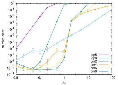
Figure 5: Median value (obtained from 10 random instances for $N=64$ and $T=4096$) of the relative error vs. step size using Dormand-Prince 5th and 8th order methods (dp5,dp8) and Cayley-Magnus method of 2nd, 4th, 6th, and 8th order (cm2,cm4,cm6,cm8).

Fig. 5 compares the relative errors for ground state probability of random instances with $N=64$ and $T=4096$ as a function of step size, obtained using various integrators. Cayley-Magnus method achieves the best performance. Python code (version 3.5 or above, using NumPy and SciPy packages) implementing the integration method is presented on the next page.

Python reference implementation

import sys
from numpy import *
from scipy import sparse as sp, linalg as la

# Banded matrix multiplication
def bxb(A,B):
    d=(size(A,0)-1)//2
    C=A*B[d,:]
    for s in r_[-d:0]: C[:s,-s:]+=A[-s:,:s]*B[d+s,-s:]
    for s in r_[:d]+1: C[s:,:-s]+=A[:-s,s:]*B[d+s,:-s]
    return C

# Main routine
def solve(G,J,t1,t2,T,p=4,dt=1.0):
    if (J[0]!=0): sys.exit(’Use open BCs’)
    if (p>4): sys.exit(’Use p<=4’)

    N=len(J)
    k=r_[:p]; s=roots(r_[1,cumprod(-(p+k+1)*(p-k)/(k+1))])

    t1/=T; t2/=T; dt/=T; G*=T; J*=T
    dt=(t2-t1)/ceil((t2-t1)/dt)

    d=2*p-1
    I=zeros((2*d+1,2*N)); I[d,:]=1
    A=zeros((2*d+1,2*N)); A[d-1,1::2]=2*G; A[d+1,::2]=-2*G
    B=zeros((2*d+1,2*N)); B[d-1,2::2]=2*J[1:]; B[d+1,1:-1:2]=-2*J[1:]

    D=(B-A)*dt**2
    C=(bxb(A,B)-bxb(B,A))*dt**3

    S=eye(2*N); t=t1+dt/2
    while t<t2:
        H=((1-t)*A+t*B)*dt
        W=H
        if p>=2:
            W+=-(1/12)*C
        if p>=3:
            DC=bxb(D,C)-bxb(C,D)
            HC=bxb(H,C)-bxb(C,H)
            HHC=bxb(H,HC)-bxb(HC,H)
            W+=-(1/240)*DC+(1/720)*HHC
        if p>=4:
            DDC=bxb(D,DC)-bxb(DC,D)
            HDC=bxb(H,DC)-bxb(DC,H)
            HHDC=bxb(H,HDC)-bxb(HDC,H)
            DHHC=bxb(D,HHC)-bxb(HHC,D)
            HHHC=bxb(H,HHC)-bxb(HHC,H)
            HHHHC=bxb(H,HHHC)-bxb(HHHC,H)
            W+=-(1/6720)*DDC-(1/30240)*HHDC+(1/7560)*DHHC-(1/30240)*HHHHC
        for sk in s:
            S=sp.spdiags(sk*I+W,r_[d:-d-1:-1],2*N,2*N)@S
            S=la.solve_banded((d,d),sk*I-W,S)
        S=real(S)
        t+=dt
    return U