Optimization of the Mean First Passage Time in Near-Disk and Elliptical Domains in 2-D with Small Absorbing Traps

Abstract

The determination of the mean first passage time (MFPT) for a Brownian particle in a bounded 2-D domain containing small absorbing traps is a fundamental problem with biophysical applications. The average MFPT is the expected capture time assuming a uniform distribution of starting points for the random walk. We develop a hybrid asymptotic-numerical approach to predict optimal configurations of $m$ small stationary circular absorbing traps that minimize the average MFPT in near-disk and elliptical domains. For a general class of near-disk domains, we illustrate through several specific examples how simple, but yet highly accurate, numerical methods can be used to implement the asymptotic theory. From the derivation of a new explicit formula for the Neumann Green’s function and its regular part for the ellipse, a numerical approach based on our asymptotic theory is used to investigate how the spatial distribution of the optimal trap locations changes as the aspect ratio of an ellipse of fixed area is varied. The results from the hybrid theory for the ellipse are compared with full PDE numerical results computed from the closest point method [10]. For long and thin ellipses, it is shown that the optimal trap pattern for $m=2,\ldots,5$ identical traps is collinear along the semi-major axis of the ellipse. For such essentially 1-D patterns, a thin-domain asymptotic analysis is formulated and implemented to accurately predict the optimal locations of collinear trap patterns and the corresponding optimal average MFPT.

1 Introduction

The concept of first passage time arises in various applications in biology, biochemistry, ecology, physics, and biophysics (see [6], [7], [20], [15] [23], [21], and the references therein). Narrow escape or capture problems are first passage time problems that characterize the expected time it takes for a Brownian “particle” to reach some absorbing set of small measure. These problems are of singular perturbation type as they involve two spatial scales: the ${\mathcal{O}}(1)$ spatial scale of the confining domain and the ${\mathcal{O}}(\varepsilon)$ asymptotically small scale of the absorbing set. Narrow escape and capture problems arise in various applications, including estimating the time it takes for a receptor to hit a certain target binding site, the time it takes for a diffusing surface-bound molecules to reach a localized signaling region on the cell membrane, or the time it takes for a predator to locate its prey, among others (cf. [1], [2], [4], [3], [9], [16], [24], [19], [15]). A comprehensive overview of the applications of narrow escape and capture problems in cellular biology is given in [8].

In this paper, we consider a narrow capture problem that involves determining the MFPT for a Brownian particle, confined in a bounded two-dimensional domain, to reach one of $m$ small stationary circular absorbing traps located inside the domain. The average MFPT for this diffusion process is the expected time for capture given a uniform distribution of starting points for the random walk. In the limit of small trap radius, this narrow capture problem can be analyzed by techniques in strong localized perturbation theory (cf. [26], [27]). For a disk-shaped domain spatial configurations of small absorbing traps that minimize the average MFPT domain were identified in [12]. However, the problem of identifying optimal trap configurations in other geometries is largely open. In this direction, the specific goal of this paper is to develop and implement a hybrid asymptotic-numerical theory to identify optimal trap configurations in near-disk domains and in the ellipse.

In § 2, we use a perturbation approach to derive a two-term approximation for the average MFPT in a class of near-disk domains in terms of a boundary deformation parameter $\sigma\ll 1$. In our analysis, we allow for a smooth, but otherwise arbitrary, star-shaped perturbation of the unit disk that preserves the domain area. At each order in $\sigma$, an approximate solution is derived for the MFPT that is accurate to all orders in $\nu\equiv{-1/\log\varepsilon}$, where $\varepsilon\ll 1$ is the common radius of the $m$ circular absorbing traps contained in the domain. To leading-order in $\sigma$, this small-trap singular perturbation analysis is formulated in the unit disk and leads to a linear algebraic system for the leading-order average MFPT involving the Neumann Green’s matrix. At order ${\mathcal{O}}(\sigma)$, a further linear algebraic system that sums all logarithmic terms in $\nu$ is derived that involves the Neumann Green’s matrix and certain weighted integrals of the boundary profile characterizing the domain perturbation. In § 3, we show how to numerically implement this asymptotic theory by using the analytical expression for the Neumann Green’s function for the unit disk together with the trapezoidal rule to compute certain weighted integrals of the boundary profile with high precision. From this numerical implementation of our asymptotic theory, and combined with either a simple gradient descent procedure or a particle swarming approach [11], we can numerically identify optimal trap configurations that minimize the average MFPT in near-disk domains. In § 3.1, we illustrate our hybrid asymptotic-numerical framework by determining some optimal trap configurations in various specific near-disk domains.

For a general 2-D domain containing small absorbing traps, a singular perturbation analysis in the limit of small trap radii, related to that in [15], [4], [12], and [26], shows that the average MFPT is closely approximated by the solution to a linear algebraic system involving the Neumann Green’s matrix. The challenge in implementing this analytical theory is that, for an arbitrary 2-D domain, a full PDE numerical solution of the Neumann Green’s function and its regular part is typically required to calculate this matrix. However, for an elliptical domain, in (4.36) and (4.37) below, we provide a new explicit representation of this Neumann Green’s function and its regular part. These explicit formulae allow for a rapid numerical evaluation of the Neumann Green’s interaction matrix for a given spatial distribution of the centers of the circular traps in the ellipse. The linear algebraic system determining the average MFPT is then coupled to a gradient descent numerical procedure in order to readily identify optimal trap configurations that minimize the average MFPT in an ellipse. Although, a similar formula for the Neumann Green’s function has been derived previously for a rectangular domain (cf. [17], [18], [14]), and an explicit and simple formula exists for the disk [12], to our knowledge there has been no prior derivation of a rapidly converging infinite series representation for the Neumann Green’s function in an ellipse. The derivation of this Neumann Green’s function using elliptic cylindrical coordinates is deferred until § 5.

With this explicit approach to determine the Neumann Green’s matrix, in § 4 we develop a hybrid asymptotic-numerical framework to approximate optimal trap configurations that minimize the average MFPT in an ellipse of a fixed area. In § 4.1 we implement our hybrid method to investigate how the optimal trap patterns change as the aspect ratio of the ellipse is varied. The results from the hybrid theory for the ellipse are favorably compared with full PDE numerical results computed from a computationally intensive numerical procedure of using the closest point method [10] to compute the average MFPT and a particle swarming approach [11] to numerically identify the optimum trap configuration. As the ellipse becomes thinner, our hybrid theory shows that the optimal trap pattern for $m=2,\ldots,5$ identical traps becomes collinear along the semi-major axis of the ellipse. In the limit of a long and thin ellipse, in § 4.2 a thin-domain asymptotic analysis is formulated and implemented to accurately predict the optimal locations of collinear trap configurations and the corresponding optimal average MFPT.

In § 6, we show that the optimal trap configurations that minimize the average MFPT also correspond to trap patterns that maximize the coefficient of order ${\mathcal{O}}(\nu^{2})$ in the asymptotic expansion of the fundamental Neumann eigenvalue of the Laplacian in the perforated domain. This fundamental eigenvalue characterizes the rate of capture of the Brownian particle by the traps. Eigenvalue optimization problems for the fundamental Neumann eigenvalue in a domain with small absorbing traps have been studied in [12] for the unit disk. The results herein extend this previous analysis to the ellipse and to near-disk domains.

2 Asymptotics of the MFPT in Near-Disk Domains

We derive an asymptotic approximation for the MFPT for a class of near-disk 2-D domains that are defined in polar coordinates by

(2.1) $$\Omega_{\sigma}=\Big{\{}(r,\theta)\,\Big{|}\,0<r\leq 1+\sigma h(\theta)\,,\,\,0\leq\theta\leq 2\pi\Big{\}}\,,$$

where the boundary profile, $h(\theta)$, is assumed to be an ${\mathcal{O}}(1)$, $C^{\infty}$ smooth $2\pi$ periodic function with $\int_{0}^{2\pi}h(\theta)\,d\theta=0$. Observe that $\Omega_{\sigma}\to\Omega$ as $\sigma\to 0$, where $\Omega$ is the unit disk. Since $\int_{0}^{2\pi}h(\theta)\,d\theta=0$, the domain area $|\Omega_{\sigma}|$ for $\sigma\ll 1$ is $|\Omega_{\sigma}|=\pi+{\mathcal{O}}(\sigma^{2})$.

Inside the perturbed disk $\Omega_{\sigma}$, we assume that there are $m$ circular traps of a common radius $\varepsilon\ll 1$ that are centered at arbitrary locations $\mathbf{x}_{1},\ldots,\mathbf{x}_{m}$ with $|\mathbf{x}_{i}-\mathbf{x}_{j}|={\mathcal{O}}(1)$ and $\mbox{dist}(\partial\Omega_{\sigma},\mathbf{x}_{j})={\mathcal{O}}(1)$ as $\varepsilon\to 0$. The $j$-th trap, centered at some $\mathbf{x}_{j}\in\Omega_{\sigma}$, is labelled by $\Omega_{\varepsilon j}=\{\mathbf{x}:|\mathbf{x}-\mathbf{x}_{j}|\leq\varepsilon\}$. The near-disk domain with the union of the trap regions deleted is denoted by $\bar{\Omega}_{\sigma}$. In $\bar{\Omega}_{\sigma}$, it is well-known that the mean first passage time (MFPT) for a Brownian particle starting at a point $\mathbf{x}\in\bar{\Omega}_{\sigma}$ to be absorbed by one of the traps satisfies (cf. [20])

(2.2) $$\begin{split}D\,\Delta u=-1\,,&\quad\mathbf{x}\in\bar{\Omega}_{\sigma}\,;\qquad\bar{\Omega}_{\sigma}\equiv\Omega_{\sigma}\setminus\cup_{j=1}^{m}\Omega_{\varepsilon j}\,,\\ \partial_{n}u=0\,,\quad\mathbf{x}\in\partial\Omega_{\sigma}\,;&\qquad u=0\,,\quad\mathbf{x}\in\partial\Omega_{\varepsilon j}\,,\quad j=1,\ldots,m\,.\end{split}$$

In terms of polar coordinates, the Neumann boundary condition in (2.2) becomes

(2.3) $$\begin{split}u_{r}-&\frac{\sigma h_{\theta}}{(1+\sigma h)^{2}}u_{\theta}=0\quad\text{on}\quad r=1+\sigma h(\theta)\,.\end{split}$$

For an arbitrary arrangement $\{{\mathbf{x}_{1},\ldots,\mathbf{x}_{m}\}}$ of the centers of the traps, and for $\sigma\to 0$ and $\varepsilon\to 0$, we will derive a reduced problem consisting of two linear algebraic systems that provide an asymptotic approximation to the MFPT that has an error ${\mathcal{O}}(\sigma^{2},\varepsilon^{2})$. These linear algebraic systems involve the Neumann Green’s matrix and certain weighted integrals of the boundary profile $h(\theta)$.

To analyze (2.2), we use a regular perturbation series to approximate (2.2) for the near-disk domain to problems involving a unit disk. We expand the MFPT $u$ as

(2.4) $$\begin{split}u=u_{0}+\sigma u_{1}+\ldots\,,\end{split}$$

and substitute it into (2.2) and (2.3). This yields the leading-order problem

(2.5) $$\begin{split}D\,\Delta u_{0}=-1\,,&\quad\mathbf{x}\in\bar{\Omega}\,;\qquad\bar{\Omega}\equiv\Omega\setminus\cup_{j=1}^{m}\Omega_{\varepsilon j}\,,\\ \partial_{n}u_{0}=0\,,\quad\text{on}\quad r=1\,;&\qquad u_{0}=0\,,\quad\mathbf{x}\in\partial\Omega_{\varepsilon j}\,,\quad j=1,\ldots,m\,,\end{split}$$

together with the following problem for the next order correction $u_{1}$:

(2.6) $$\begin{split}\Delta u_{1}=0\,,&\quad\mathbf{x}\in\bar{\Omega}\,;\qquad\partial_{r}u_{1}=-hu_{0rr}+h_{\theta}u_{0\theta}\,,\quad\text{on}\quad r=1\,;\\ \quad u_{1}&=0\,,\quad\mathbf{x}\in\partial\Omega_{\varepsilon j}\,,\quad j=1,\ldots,m\,.\end{split}$$

Observe that (2.5) and (2.6) are formulated on the unit disk and not on the perturbed disk. Assuming $\varepsilon^{2}\ll\sigma$, we use (2.4) and $|\Omega_{\sigma}|=|\Omega|+{\mathcal{O}}(\sigma^{2})$ to derive an expansion for the average MFPT, defined by $\overline{u}\equiv\frac{1}{|\bar{\Omega}_{\sigma}|}\int_{\bar{\Omega}_{\sigma}}u\,\text{d}\mathbf{x}$, in the form

(2.7) $$\begin{split}\overline{u}=\frac{1}{|\Omega|}\int_{\Omega}u_{0}\,\text{d}\mathbf{x}+\sigma\left[\frac{1}{|\Omega|}\int_{\Omega}u_{1}\,\text{d}\mathbf{x}+\frac{1}{|\Omega|}\int_{0}^{2\pi}h(\theta)\,u_{0}|_{r=1}\,\text{d}\theta\right]+\mathcal{O}(\sigma^{2},\varepsilon^{2})\,,\end{split}$$

where $|\Omega|=\pi$ and $u_{0}|_{r=1}$ is the leading-order solution $u_{0}$ evaluated on $r=1$.

Since the asymptotic calculation of the leading-order solution $u_{0}$ by the method of matched asymptotic expansions in the limit $\varepsilon\to 0$ of small trap radius was done previously in [4] (see also [15] and [26]), we only briefly summarize the analysis here. In the inner region near the $j$-th trap, we define the inner variables $\mathbf{y}=\varepsilon^{-1}(\mathbf{x}-\mathbf{x}_{j})$ and $u_{0}(\mathbf{x})=v_{j}(\varepsilon\mathbf{y}+\mathbf{x}_{j})$ with $\rho=|\mathbf{y}|$, for $j=1,\ldots,m$. Upon writing (2.5) in terms of these inner variables, we have for $\varepsilon\to 0$ and for each $j=1,\ldots,m$ that

(2.8) $$\begin{split}\Delta_{\rho}\,v_{j}&=0\,,\quad\rho>1\,;\qquad v_{j}=0\,,\quad\mbox{on}\,\,\,\rho=1\,,\end{split}$$

where $\Delta_{\rho}\equiv\partial_{\rho\rho}+\rho^{-1}\partial_{\rho}$. This admits the radially symmetric solution $v_{j}=A_{j}\log\rho$, where $A_{j}$ is an unknown constant. From an asymptotic matching of the inner and outer solutions we obtain the required singularity condition for the outer solution $u_{0}$ as $\mathbf{x}\to\mathbf{x}_{j}$ for $j=1,\ldots,m$. In this way, we obtain that $u_{0}$ satisfies

(2.9a) $$\Delta u_{0}=-{1/D}\,,\quad\mathbf{x} \in\Omega\setminus\{{\mathbf{x}_{1},\ldots,\mathbf{x}_{m}\}}\,;\quad\partial_{r}u_{0}=0\,,\,\,\,\mathbf{x}\in\partial\Omega\,;$$

(2.9b) $$u_{0}\sim A_{j}\log|\mathbf{x}-\mathbf{x}_{j}| +A_{j}/\nu\quad\text{as}\quad\mathbf{x}\to\mathbf{x}_{j}\,,\qquad j=1,\ldots,m\,,$$

where $\nu\equiv-1/\log\varepsilon$. In terms of the Delta distribution, (2.9) implies that

(2.10) $$\Delta u_{0}=-\frac{1}{D}+2\pi\sum_{j=1}^{m}A_{j}\delta(\mathbf{x}-\mathbf{x}_{j})\,,\quad\mathbf{x}\in\Omega\,;\qquad\partial_{r}u_{0}=0\,,\,\,\,\mathbf{x}\in\partial\Omega\,.$$

By applying the divergence theorem to (2.10) over the unit disk we obtain that $\sum_{j=1}^{m}A_{j}={|\Omega|/(2\pi D)}$. The solution to (2.10) is represented as

(2.11) $$u_{0}=-2\pi\sum_{k=1}^{m}A_{k}G(\mathbf{x};\mathbf{x}_{k})+\overline{u}_{0}\,;\qquad\overline{u}_{0}=\frac{1}{|\Omega|}\int_{\Omega}u_{0}\,\text{d}\mathbf{x}\,,$$

where $G(\mathbf{x};\mathbf{x}_{j})$ is the Neumann Green’s function for the unit disk, which satisfies

(2.12a) $$\Delta G=\frac{1}{|\Omega|}-\delta(\mathbf{x}-\mathbf{x}_{j})\,,\quad\mathbf{x}\in\Omega\,;\quad\partial_{n}G=0\,,\,\,\,\mathbf{x}\in\partial\Omega\,;\quad\int_{\Omega}G\,\text{d}\mathbf{x}=0\,,$$

(2.12b) $$G\sim-\frac{1}{2\pi}\log{|\mathbf{x}-\mathbf{x}_{j}|}+R_{j}+\nabla_{\mathbf{x}}R_{j}\cdot(\mathbf{x}-\mathbf{x}_{j})\quad\text{as}\quad\mathbf{x}\to\mathbf{x}_{j}\,.$$

Here, $R_{j}\equiv R(\mathbf{x}_{j})$ is the regular part of the Green’s function at $\mathbf{x}=\mathbf{x}_{j}$. Expanding (2.11) as $\mathbf{x}\to\mathbf{x}_{j}$, and using the singularity behaviour of $G(\mathbf{x};\mathbf{x}_{j})$ given in (2.12b), together with the far-field behavior (2.9b) for $u_{0}$, we obtain the matching conditon:

(2.13) $$-2\pi A_{j}\,R_{j}-2\pi\sum_{i\neq j}^{m}A_{i}\,G(\mathbf{x}_{j};\mathbf{x}_{i})+\overline{u}_{0}\sim{A_{j}/\nu}\,,\qquad\mbox{for}\quad j=1,\ldots,m\,.$$

This yields a linear algebraic system for $\overline{u}_{0}$ and $\mathcal{A}\equiv(A_{1},\ldots,A_{m})^{T}$, given by

(2.14) $$(I+2\pi\nu\,\mathcal{G})\mathcal{A}=\nu\,\overline{u}_{0}\,\mathbf{e}\,,\qquad\mathbf{e}^{T}\mathcal{A}=\frac{|\Omega|}{2\pi D}\,.$$

Here, $\mathbf{e}\equiv(1,\ldots,1)^{T}$, $\nu=-1/\log\varepsilon$, $I$ is the $m\times m$ identity matrix, and $\mathcal{G}$ is the symmetric Green’s matrix with matrix entries given by

(2.15) $$(\mathcal{G})_{jj}=R_{j}\,\,\,\text{for}\,\,\,i=j\quad\text{and}\quad(\mathcal{G})_{ij}=(\mathcal{G})_{ji}=G(\mathbf{x}_{i};\mathbf{x}_{j})\,\,\,\text{for}\,\,\,i\neq j\,.$$

We left-multiply the equation for $\mathcal{A}$ in (2.14) by $\mathbf{e}^{T}$, which isolates $\overline{u}_{0}$. By using this expression in (2.14), and defining the matrix $E$ by $E={\mathbf{e}\mathbf{e}^{T}/m}$, we get

(2.16) $$\Big{[}I+2\pi\nu(I-E)\mathcal{G}\Big{]}\mathcal{A}=\frac{|\Omega|}{2\pi Dm}\mathbf{e}\,,\quad\text{and}\quad\overline{u}_{0}=\frac{|\Omega|}{2\pi D\nu m}+\frac{2\pi}{m}\mathbf{e}^{T}\mathcal{G}\mathcal{A}\,.$$

Remark 2.1.

The result (2.16) effectively sums all the logarithmic terms in powers of $\nu={-1/\log\varepsilon}$. To estimate the error with this approximation with regards to the leading-order in $\sigma$ problem (2.5), we calculate using (2.11) the refined local behavior

(2.17) $$u_{0}\sim-2\pi\left(A_{j}\,R_{j}+\sum_{i\neq j}^{m}A_{i}\,G(\mathbf{x}_{j};\mathbf{x}_{i})\right)+\overline{u}_{0}+\mathbf{f}_{j}\cdot(\mathbf{x}-\mathbf{x}_{j})\,,\quad\mbox{as}\quad\mathbf{x}\to\mathbf{x}_{j},$$

where $\mathbf{f}_{j}\equiv-2\pi\left(A_{j}\nabla_{\mathbf{x}}R_{j}+\sum_{i\neq j}^{m}A_{i}\,\nabla_{\mathbf{x}}G(\mathbf{x};\mathbf{x}_{i})|_{\mathbf{x}=\mathbf{x}_{j}}\right)$. To account for this gradient term, near the $j$-th trap we must modify the inner expansion as $v_{j}\sim A_{j}\log\rho+\varepsilon v_{j1}$. Here $\Delta_{\mathbf{y}}v_{j1}=0$ in $|\mathbf{y}|\geq 1$, with $v_{j1}=0$ on $|\mathbf{y}|=1$ and $v_{j1}\sim\mathbf{f}_{j}\cdot\mathbf{y}$ as $|\mathbf{y}|\to\infty$. The solution is $v_{j1}=\mathbf{f}_{j}\cdot\left(\mathbf{y}-{\mathbf{y}/|\mathbf{y}|^{2}}\right)$. The far field behavior for $v_{j1}$ implies that in the outer region we must have that $u\sim u_{0}+\varepsilon^{2}w_{0}+\cdots$, where $w_{0}\sim-\mathbf{f}_{j}\cdot{(\mathbf{x}-\mathbf{x}_{j})/|\mathbf{x}-\mathbf{x}_{j}|^{2}}$ as $\mathbf{x}\to\mathbf{x}_{j}$. This shows that the $\varepsilon$-error estimate for $u_{0}$ is ${\mathcal{O}}(\varepsilon^{2})$, as claimed in (2.7).

Next, we study the $\mathcal{O}(\sigma)$ problem for $u_{1}$ given in (2.6). We construct an inner region near each of the traps by introducing the inner variables $\mathbf{y}=\varepsilon^{-1}(\mathbf{x}-\mathbf{x}_{j})$ and $u_{1}(\mathbf{x})=V_{j}(\varepsilon\mathbf{y}+\mathbf{x}_{j})$ with $\rho=|\mathbf{y}|$. From (2.6), this yields the same leading-order inner problem (2.8) with $v_{j}$ replaced by $V_{j}$. The radially symmetric solution is $V_{j}=B_{j}\log\rho$, where $B_{j}$ is a constant to be found. By matching this far-field behavior of the inner solution to the outer solution we obtain the singularity behavior for $u_{1}$ as $\mathbf{x}\to\mathbf{x}_{j}$ for $j=1,\ldots,m$. In this way, we find from (2.6) that $u_{1}$ satisfies

(2.18a) $$\Delta u_{1} =0\,,\quad\mathbf{x}\in\Omega\setminus\{\mathbf{x}_{1},\ldots,\mathbf{x}_{m}\}\,;\quad\partial_{r}u_{1}=F(\theta)\,,\quad\text{on}\quad r=1;$$

(2.18b) $$u_{1} \sim B_{j}\log{|\mathbf{x}-\mathbf{x}_{j}|}+B_{j}/\nu\quad\text{as}\quad\mathbf{x}\to\mathbf{x}_{j}\quad j=1,\ldots,m\,,$$

where $$\nu=-1/\log\varepsilon F(\theta)$$ and is defined by

(2.18c) $$F(\theta)\equiv-hu_{0rr}|_{r=1}+h_{\theta}u_{0\theta}|_{r=1}=\left(hu_{0\theta}\right)_{\theta}+\frac{h}{D}\,.$$

In deriving (2.18c) we used $$u_{0rr}=-u_{0\theta\theta}+{1/D} r=1$$ at , as obtained from (2.5).

Next, we introduce the Dirac distribution and write the problem (2.18) for $u_{1}$ as

(2.19) $$\Delta u_{1}=2\pi\sum_{i=1}^{m}B_{i}\,\,\delta(\mathbf{x}-\mathbf{x}_{i})\,,\quad\mathbf{x}\in\Omega\,;\qquad u_{1r}=F(\theta)\,,\quad\text{on}\quad r=1\,.$$

Since $\int_{0}^{2\pi}F(\theta)\,\text{d}\theta=0$, the divergence theorem yields $\sum_{j=1}^{m}B_{j}=0$. We decompose

(2.20) $$u_{1}=-2\pi\sum_{i=1}^{m}B_{i}G(\mathbf{x};\mathbf{x}_{i})+u_{1p}+\overline{u}_{1}\,,$$

where $\overline{u}_{1}$ is the unknown average of $u_{1}$ over the unit disk, and $G(\mathbf{x};\mathbf{x}_{i})$ is the Neumann Green’s function satisfying (2.12). Here, $u_{1p}$ is taken to be the unique solution to

(2.21) $$\Delta u_{1p} =0,\quad\mathbf{x}\in\Omega;\quad\partial_{r}u_{1p}=F(\theta)\,\quad\text{on}\quad r=1;\quad\int_{\Omega}u_{1p}\,\text{d}\mathbf{x}=0\,.$$

Next, by expanding (2.20) as $\mathbf{x}\to\mathbf{x}_{j}$, we use the singularity behaviour of $G(\mathbf{x};\mathbf{x}_{j})$ as given in (2.12b) to obtain the local behavior of $u_{1}$ as $\mathbf{x}\to\mathbf{x}_{j}$, for each $j=1,\ldots,m$. The asymptotic matching condition is that this behavior must agree with that given in (2.18b). In this way, we obtain a linear algebraic system for the constant $\overline{u}_{1}$ and the vector $\mathbf{B}=(B_{1},\ldots,B_{m})^{T}$, which is given in matrix form by

(2.22) $$(I+2\pi\nu\mathcal{G})\mathbf{B}=\nu\overline{u}_{1}\mathbf{e}+\nu\mathbf{u}_{1p}\,,\qquad\mathbf{e}^{T}\mathbf{B}=0\,.$$

Here, $I$ is the identity, $\mathbf{e}=(1,\ldots,1)^{T}$, and $\mathbf{u}_{1p}=(u_{1p}(\mathbf{x}_{1}),\ldots,u_{1p}(\mathbf{x}_{m}))^{T}$. Next, we left multiply the equation for $\mathbf{B}$ by $\mathbf{e}^{T}$. This determines $\overline{u}_{1}$, which is then re-substituted into (2.22) to obtain the uncoupled problem

(2.23) $$\Big{[}I+2\pi\nu(I-E)\mathcal{G}\Big{]}\mathbf{B}=\nu(I-E)\mathbf{u}_{1p}\,,\quad\text{and}\quad\overline{u}_{1}=-\frac{1}{m}\mathbf{e}^{T}\mathbf{u}_{1p}+\frac{2\pi}{m}\mathbf{e}^{T}\mathcal{G}\mathbf{B}\,,$$

where $E\equiv{\mathbf{e}\mathbf{e}^{T}/m}$. Since $\mathbf{e}^{T}(I-E)=0$, we observe from (2.23) that $\mathbf{e}^{T}\mathbf{B}=0$, as required. Equation (2.23) gives a linear system for the $\mathcal{O}(\sigma)$ average MFPT $\overline{u}_{1}$ in terms of the Neumann Green’s matrix $\mathcal{G}$, and the vector $\mathbf{u}_{1p}$.

To determine $u_{1p}(\mathbf{x}_{j})$, we use Green’s second identity on (2.21) and (2.12) to obtain a line integral over the boundary $\mathbf{x}\in\partial\Omega$ of the unit disk. Then, by using (2.18c) for $F(\theta)$, integrating by parts and using $2\pi$ periodicity we get

(2.24) $$u_{1p}(\mathbf{x}_{j})=\int_{0}^{2\pi}G(\mathbf{x};\mathbf{x}_{j})F(\theta)\,d\theta=\int_{0}^{2\pi}G(\mathbf{x};\mathbf{x}_{j})\frac{h(\theta)}{D}\,d\theta-\int_{0}^{2\pi}h(\theta)u_{0\theta}\partial_{\theta}G(\mathbf{x};\mathbf{x}_{j})\,d\theta\,.$$

Then, by setting (2.11) for $u_{0}$ into (2.24), we obtain in terms of the $A_{k}$ of (2.16) that

(2.25a) $$u_{1p}(\mathbf{x}_{j})=\frac{1}{D}\int_{0}^{2\pi}G(\mathbf{x};\mathbf{x}_{j})h(\theta)\,d\theta+2\pi\sum_{k=1}^{m}A_{k}J_{jk}\,.$$

Here, $$J_{jk} \mathbf{x}=(\cos(\theta),\sin(\theta))^{T}$$ is defined by the following boundary integral with :

(2.25b) $$J_{jk}\equiv\int_{0}^{2\pi}h(\theta)\left(\partial_{\theta}G(\mathbf{x};\mathbf{x}_{j})\right)\left(\partial_{\theta}G(\mathbf{x};\mathbf{x}_{k})\right)\,d\theta\,.$$

¿From a numerical evaluation of the boundary integrals in (2.25), we can calculate $\mathbf{u}_{1p}=(u_{1p}(\mathbf{x}_{1}),\ldots,u_{1p}(\mathbf{x}_{m}))^{T}$, which specifies the right-hand side of the linear system (2.23) for $\mathbf{B}$. After determining $\mathbf{B}$, we obtain $\overline{u}_{1}$ from the second relation in (2.23). Finally, by substituting (2.11) for $u_{0}$ into (2.7), and recalling that $\int_{0}^{2\pi}h(\theta)\,d\theta=0$, we obtain a two-term expansion for the average MFPT given by

(2.26) $$\overline{u}\sim\overline{u}_{0}+\sigma\left(\overline{u}_{1}-2\sum_{k=1}^{m}A_{k}\int_{0}^{2\pi}G(\mathbf{x};\mathbf{x}_{k})h(\theta)\,d\theta\right)\,.$$

Here, $\mathbf{x}\in\partial\Omega$ and $\overline{u}_{0}$ is determined from (2.16).

3 Optimizing Trap Configurations for the MFPT in the Near-Disk

To numerically evaluate the boundary integrals in (2.25) and (2.26), we need explicit formulae for $G(\mathbf{x};\mathbf{x}_{j})$ and $\partial_{\theta}G(\mathbf{x};\mathbf{x}_{j})$ on the boundary of the unit disk where $\mathbf{x}=(\cos\theta,\sin\theta)^{T}$. For the unit disk, we obtain from equation (4.3) of [12] that

(3.27a) $$G(\mathbf{x};\mathbf{x}_{j})=-\frac{1}{2\pi}\log|\mathbf{x}-\mathbf{x}_{j}|-\frac{1}{4\pi}\log\left(|\mathbf{x}|^{2}|\mathbf{x}_{j}|^{2}+1-2\mathbf{x}\cdot\mathbf{x}_{j}\right)+\frac{(|\mathbf{x}|^{2}+|\mathbf{x}_{j}|^{2})}{4\pi}-\frac{3}{8\pi},$$

(3.27b) $$R(\mathbf{x}_{j};\mathbf{x}_{j})=-\frac{1}{2\pi}\log\left(1-|\mathbf{x}_{j}|^{2}\right)+\frac{|\mathbf{x}_{j}|^{2}}{2\pi}-\frac{3}{8\pi}\,.$$

For an arbitrary configuration $\{{\mathbf{x}_{1},\ldots,\mathbf{x}_{m}\}}$ of traps, these expressions can be used to evaluate the Neumann Green’s matrix $\mathcal{G}$ of (2.15) as needed in (2.16) and (2.23).

Next, by setting $\mathbf{x}=(\cos\theta,\sin\theta)^{T}$ we can evaluate $G(\mathbf{x};\mathbf{x}_{j})$ on $\partial\Omega$, and then calculate its tangential boundary derivative $\partial_{\theta}G(\mathbf{x};\mathbf{x}_{j})$. By using (3.27a), we obtain

(3.28a) $$G(\mathbf{x};\mathbf{x}_{j}) =-\frac{1}{2\pi}\log\left(1+r_{j}^{2}-2r_{j}\cos(\theta-\theta_{j})\right)+\frac{1}{4\pi}(1+r_{j}^{2})-\frac{3}{8\pi}\,,$$

(3.28b) $$\partial_{\theta}G(\mathbf{x};\mathbf{x}_{j}) =-\frac{r_{j}}{\pi}\frac{\sin(\theta-\theta_{j})}{\left[r_{j}^{2}+1-2r_{j}\cos(\theta-\theta_{j})\right]}\,,$$

where $r_{j}\equiv|\mathbf{x}_{j}|$ and $\mathbf{x}_{j}=r_{j}(\cos\theta_{j},\sin\theta_{j})^{T}$. Then, since $\int_{0}^{2\pi}h(\theta)\,d\theta=0$, we can write the two boundary integrals appearing in (2.25) and (2.26) explicitly as

(3.29a) $$\int_{0}^{2\pi}G(\mathbf{x};\mathbf{x}_{j})h(\theta)\,d\theta=-\frac{1}{2\pi}\int_{0}^{2\pi}h(\theta)\log\left(1+r_{j}^{2}-2r_{j}\cos(\theta-\theta_{j})\right)\,d\theta\,,$$

(3.29b) $$J_{jk}=\frac{r_{j}r_{k}}{\pi^{2}}\int_{0}^{2\pi}\frac{h(\theta)\sin(\theta-\theta_{j})\sin(\theta-\theta_{k})}{\left[r_{j}^{2}+1-2r_{j}\cos(\theta-\theta_{j})\right]\left[r_{k}^{2}+1-2r_{k}\cos(\theta-\theta_{k})\right]}\,d\theta\,.$$

Although for an arbitrary $h(\theta)$ the integrals in (3.29) cannot be evaluated in closed form, they can be computed to a high degree of accuracy with relatively few grid points using the trapezoidal rule since this quadrature rule is exponentially convergent for $C^{\infty}$ smooth periodic functions [25]. When $|x_{j}|<1$, the logarithmic singularities off of the axis of integration for $J_{jk}$ in (3.29) are mild and pose no particular problem. In this way, we can numerically calculate the two-term expansion (2.26) for the average MFPT with high precision.

Then, to determine the optimal trap configuration we can either use the particle swarming approach [11], or the ODE relaxation dynamics scheme

(3.30) $$\frac{d\mathbf{z}}{dt}=-\nabla_{\mathbf{z}}\overline{u}\,,\qquad\mbox{where}\quad\mathbf{z}\equiv(x_{1},y_{1},\ldots,x_{m},y_{m})^{T}\,,$$

and $\overline{u}$ is given in (2.26). Starting from an admissible initial state $\mathbf{z}|_{t=0}$, where $\mathbf{x}_{j}=(x_{j},y_{j})\in\Omega_{0}$ at $t=0$ for $j=1,\ldots,m$, the gradient flow dynamics (3.30) converges to a local minimum of $\overline{u}$. Because of our high precision in calculating $\overline{u}$, a centered difference scheme with mesh spacing $10^{-4}$ was used to estimate the gradient in (3.30).

3.1 Examples of the Theory

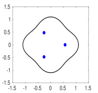
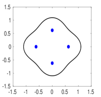
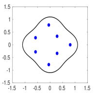
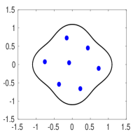
Figure 1: Optimal trap patterns for $D=1$ in a near-disk domain with boundary $r=1+\sigma\cos(4\theta)$, with $\sigma=0.1$, that contains $m$ traps of a common radius $\varepsilon=0.05$. Computed from minimizing (2.26) using the ODE relaxation scheme (3.30). Left: $m=3$, $\overline{u}\approx 0.2962$. Inter-trap computed distances are $0.9588$, $0.9588$, and $0.9540$. This result is close to the full PDE simulation results of Fig. 2. Left middle: $m=4$, $\overline{u}\approx 0.1927$. This is a ring pattern of traps with ring radius $r_{c}\approx 0.6215$. Right Middle: $m=7$, $\overline{u}\approx 0.0925$. Right: $m=7$, $\overline{u}\approx 0.0912$. The two patterns for $m=7$ give nearly the same values for $\overline{u}$, with the rightmost pattern giving a slightly lower value.

We first set $\sigma=0.1$ and consider the boundary profile $h(\theta)=\cos(N\theta)$, where $N$ is a positive integer representing the number of boundary folds. In [10], an explicit two-term expansion for the average MFPT $\overline{u}$ was derived for the special case where $m$ traps are equidistantly spaced on a ring of radius $r_{c}$, concentric within the unperturbed disk. For such a ring pattern, in Proposition 1 of [10] it was proved that when ${N/m}\notin\mathbb{Z}^{+}$, then $\overline{u}\sim\overline{u}_{0}+{\mathcal{O}}(\sigma^{2})$, as the correction at order ${\mathcal{O}}(\sigma)$ vanishes identically. Therefore, in order to determine the optimal trap pattern when ${N/m}\notin\mathbb{Z}^{+}$ we must consider arbitrary trap configurations, and not just ring patterns of traps. By minimizing (2.26) using the ODE relaxation scheme (3.30), in the left panel of Fig. 1 we show our asymptotic prediction for the optimal trap configuration for $N=4$ folds and $m=3$ traps of a common radius $\varepsilon=0.05$. The optimal pattern is not of ring-type. The corresponding results computed from the closest point method of [10], shown in Fig. 2, are very close to the asymptotic result.

In the left-middle panel of Fig. 1, we show the optimal trap pattern computed from our asymptotic theory (2.26) and (3.30) for the boundary profile $h(\theta)=\cos(4\theta)$ with $m=4$ traps and $\sigma=0.1$. The optimal pattern is now a ring pattern of traps. In this case, as predicted by Proposition 1 of [10], the optimal pattern has traps on the rays through the origin that coincide with the maxima of the domain boundary. By applying Proposition 2 of [10], the optimal perturbed ring radius has the expansion $r_{c,opt}\sim 0.5985+0.1985\sigma$. When $\sigma=0.1$, this gives $r_{c,opt}\approx 0.6184$, and compares well with the value $r_{c}\approx 0.6215$ calculated from (2.26) and (3.30).

In the two rightmost panels of Fig. 1, we show for $h(\theta)=\cos(4\theta)$ and $\sigma=0.1$, that there are two seven-trap patterns that give local minima for the average MFPT $\bar{u}_{0}$. The minimum values of $\bar{u}_{0}$ for these patterns are very similar.

Next, we construct a boundary profile with a localized protrusion, or bulge, near $\theta=0$. To this end, we define $f(\theta)\equiv-1+\beta e^{-\chi\sin^{2}\left({\theta/2}\right)}$. By using the Taylor expansion of $e^{z}$, combined with a simple identity for $\int_{0}^{2\pi}\sin^{2n}(\psi)\,d\psi$, we conclude that $\int_{0}^{2\pi}f(\theta)\,d\theta=0$ when $\beta$ is related to $\chi$ by

(3.31) $$\frac{1}{\beta}=\frac{1}{2\pi}\int_{0}^{2\pi}e^{-\chi\sin^{2}\left({\theta/2}\right)}\,d\theta=\sum_{n=0}^{\infty}\frac{(-1)^{n}\chi^{n}}{2\pi n!}\int_{0}^{2\pi}\sin^{2n}\left(\frac{\theta}{2}\right)\,d\theta=\sum_{n=0}^{\infty}(-1)^{n}\frac{\chi^{n}(2n)!}{4^{n}\left(n!\right)^{3}}\,.$$

As $\chi$ increases, the boundary deformation becomes increasingly localized near $\theta=0$.

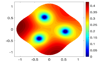
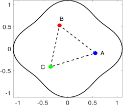
Figure 2: Optimizing a three-trap pattern, with a common trap radius $\varepsilon=0.05$, in a four-fold star-shaped domain (4-star) with boundary profile $h(\theta)=\cos(4\theta)$ and $\sigma=0.1$. Left panel: contour plot of the optimal PDE solution computed with closest point method. Right panel: optimal traps locations in the 4-star domain with computed side-lengths: $\mathbf{AB}\approx 0.9581$, $\mathbf{BC}\approx 0.9569$, and $\mathbf{CA}\approx 0.9541$. All of the computed interior angles are ${\pi/3}\pm\delta$, where $|\delta|\leq 0.0015$.

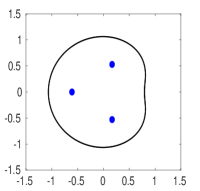
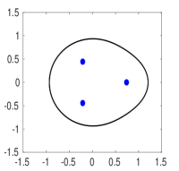
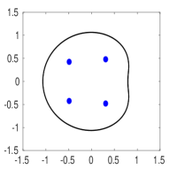
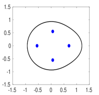
Figure 3: Optimal trap patterns for $D=1$ with $m$ traps each of radius $\varepsilon=0.05$ in a near-disk domain with boundary $r=1\pm\sigma f(\theta)$, where $\sigma=0.05$ and $f(\theta)=-1+\beta e^{-10\sin^{2}\left({\theta/2}\right)}$, with $\beta=5.4484$. Computed from minimizing (2.26) using the ODE relaxation scheme (3.30). Left: $m=3$ and inward domain bulge $r=1-\sigma f(\theta)$. Centroid of trap pattern is at $(-0.0886,0.0)$ and $\overline{u}\approx 0.2842$. Left Middle: $m=3$ and outward bulge $r=1+\sigma f(\theta)$. Centroid is at $(0.1061,0.0)$, and $\overline{u}\approx 0.2825$. Right Middle: $m=4$ and inward bulge $r=1-\sigma f(\theta)$, $\overline{u}\approx 0.1918$. Right: $m=4$ and outward bulge $r=1+\sigma f(\theta)$, $\overline{u}\approx 0.1916$.

For $\chi=10$, for which $\beta=5.4484$, in Fig. 3 we show optimal trap patterns for $m=3$ and $m=4$ traps for both an outward domain bulge, where $r=1+\sigma f(\theta)$, and an inward domain bulge, were $r=1-\sigma f(\theta)$, with $\sigma=0.05$. For the three-trap case, by comparing the two leftmost plots in Fig. 3, we observe that an inward domain bulge will displace the trap locations to the left, as expected intuitively. Alternatively, for an outward bulge, the location of the optimal trap on the line of symmetry becomes closer to the domain protrusion. An intuitive, but as we will see below in Fig. 4, naïve interpretation of the qualitative effect of this domain bulge is that it acts to confine or pin a Brownian particle in this region, and so in order to reduce the mean capture time of such a pinned particle, the best location for a trap is to move closer to the region of protrusion. For the case of four traps, a similar qualitative comparison of the optimal trap configuration for an inward and outward domain bulge is seen in the two rightmost plots in Fig. 3.

In Fig. 4, we show optimal trap patterns from our hybrid theory for $3\leq m\leq 5$ circular traps of radius $\varepsilon=0.05$ in a domain with boundary profile $r=1+\sigma h(\theta)$, where $h(\theta)=\cos(3\theta)-\cos(\theta)-\cos(2\theta)$ and $\sigma=0.075$. This boundary profile perturbs the unit disk inwards near $\theta=\pi$ and outwards near $\theta=0$. For $m=3$, in Fig. 5 we show a favorable comparison between the full numerical PDE results and the hybrid results for the optimal average MFPT and trap locations. Moreover, from the two rightmost plots in Fig. 4, we observe that there are two five-trap patterns that give local minima for $\bar{u}_{0}$. The pattern that has a trap on the line of symmetry near the outward bulge at $\theta=0$ is, in this case, not a global minimum of the average MFPT. This indicates that hard-to-assess global effects, rather than simply the local geometry near a protrusion, play a central role for characterizing the optimal trap pattern.

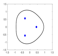
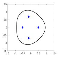
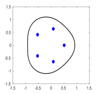
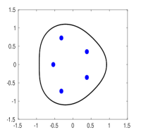
Figure 4: Optimal trap patterns for $D=1$ in a near-disk domain with boundary $r=1+\sigma h(\theta)$, $\sigma=0.075$ and $h(\theta)=\cos(3\theta)-\cos(\theta)-\cos(2\theta)$, that contains $m$ traps of a common radius $\varepsilon=0.05$. Computed from minimizing (2.26) using the ODE relaxation scheme (3.30). Left: $m=3$ and $\overline{u}\approx 0.2794$. Left-Middle: $m=4$ and $\overline{u}\approx 0.19055$. Right-Middle: $m=5$ and $\overline{u}\approx 0.1418$. Right: $m=5$, $\overline{u}\approx 0.1383$. The two patterns for $m=5$ are local minimizers, with rather close values for $\overline{u}$. The global minimum is achieved for the rightmost pattern.

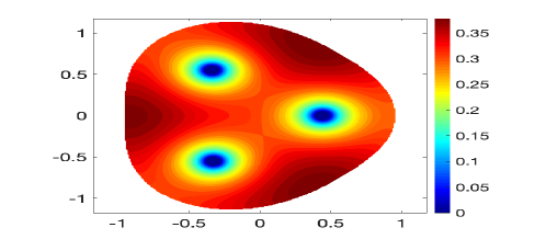
Figure 5: Contour plot of the PDE numerical solution for the optimal average MFPT and trap locations computed from the closest point method corresponding to the parameter values in the left panel of Fig. 4. Full PDE results for optimal locations: $(-0.3382,0.5512)$, $(-0.3288,-0.5510)$, $(0.4410,0.0012)$, and $\overline{u}=0.2996$. Hybrid results: $(-0.3316,0.5626)$, $(-0.3316,0.5626)$, $(0.4314,0.000)$, and $\overline{u}_{0}=0.2794$.

4 Optimizing Trap Configurations for the MFPT in an Ellipse

Next, we consider the trap optimization problem in an ellipse of arbitrary aspect ratio, but with fixed area $\pi$. Our analysis uses a new explicit analytical formula, as derived in § 5, for the Neumann Green’s function $G(\mathbf{x};\mathbf{x}_{0})$ and its regular part $R_{e}$ of (5.54).

For $m$ circular traps each of radius $\varepsilon$, the average MFPT $\overline{u}_{0}$ satisfies (see (2.16))

(4.32) $$\overline{u}_{0}=\frac{|\Omega|}{2\pi D\nu m}+\frac{2\pi}{m}\mathbf{e}^{T}\mathcal{G}\mathcal{A}\,,\quad\mbox{where}\quad\Big{[}I+2\pi\nu(I-E)\mathcal{G}\Big{]}\mathcal{A}=\frac{|\Omega|}{2\pi Dm}\mathbf{e}\,.$$

Here $E\equiv{\mathbf{e}\mathbf{e}^{T}/m}$, $\mathbf{e}=(1,\ldots,1)^{T}$, $\nu\equiv{-1/\log\varepsilon}$, and the Green’s matrix $\mathcal{G}$ depends on the trap locations $\{{\mathbf{x}_{1},\ldots,\mathbf{x}_{m}\}}$. To determine optimal trap configurations that are minimizers of the average MFPT, given in (4.32), we use the ODE relaxation scheme

(4.33) $$\frac{d\mathbf{z}}{dt}=-\nabla_{\mathbf{z}}\overline{u}_{0}\,,\qquad\mbox{where}\quad\mathbf{z}\equiv(x_{1},y_{1},\ldots,x_{m},y_{m})\,.$$

In our implementation of (4.33), the gradient was approximated using a centered difference scheme with mesh spacing $10^{-4}$. The results shown below for the optimal trap patterns are confirmed from using a particle swarm approach [11].

The derivation of the Neumann Green’s function and its regular part in § 5 is based on mapping the elliptical domain to a rectangular domain using

(4.34a) $$x=f\cosh\xi\cos\eta\,,\quad y=f\sinh\xi\sin\eta\,,\qquad f=\sqrt{a^{2}-b^{2}}\,.$$

With these elliptic cylindrical coordinates, the ellipse is mapped to the rectangle $$0\leq\xi\leq\xi_{b} 0\leq\eta\leq 2\pi a=f\cosh\xi_{b} b=f\sinh\xi_{b}$$ and , where and , so that

(4.34b) $$f=\sqrt{a^{2}-b^{2}}\,,\qquad\xi_{b}=\tanh^{-1}\left(\frac{b}{a}\right)=-\frac{1}{2}\log\beta\,,\qquad\beta\equiv\left(\frac{a-b}{a+b}\right)\,.$$

To determine $(\xi,\eta)$, given a pair $(x,y)$, we invert the transformation (4.34a) using

(4.35a) $$\xi=\frac{1}{2}\log\left(1-2s+2\sqrt{s^{2}-s}\right)\,,\quad s\equiv\frac{-\mu-\sqrt{\mu^{2}+4f^{2}y^{2}}}{2f^{2}}\,,\quad\mu\equiv x^{2}+y^{2}-f^{2}\,.$$

To recover $$\eta \eta_{\star}\equiv\sin^{-1}(\sqrt{p})$$, we define and use

(4.35b) $$\eta=\begin{cases}\eta_{\star},&\text{if }x\geq 0\,,\,\,y\geq 0\\ \pi-\eta_{\star},&\text{if }x<0\,,\,\,y\geq 0\\ \pi+\eta_{\star},&\text{if }x\leq 0\,,\,\,y<0\\ 2\pi-\eta_{\star},&\text{if }x>0\,,\,\,y<0\end{cases}\,,\quad\mbox{where}\quad p\equiv\frac{-\mu+\sqrt{\mu^{2}+4f^{2}y^{2}}}{2f^{2}}\,.$$

As derived in § 5, the matrix entries in $\mathcal{G}$ are obtained from the explicit result

(4.36a) $$\begin{split}G(\mathbf{x};\mathbf{x}_{0})&=\frac{1}{4|\Omega|}\left(|\mathbf{x}|^{2}+|\mathbf{x}_{0}|^{2}\right)-\frac{3}{16|\Omega|}(a^{2}+b^{2})-\frac{1}{4\pi}\log\beta-\frac{1}{2\pi}\xi_{>}\\ &\qquad-\frac{1}{2\pi}\sum_{n=0}^{\infty}\log\left(\displaystyle\prod_{j=1}^{8}|1-\beta^{2n}z_{j}|\right)\,,\quad\mbox{for}\quad\mathbf{x}\neq\mathbf{x}_{0}\,,\end{split}$$

where $$|\Omega|=\pi ab \xi_{>}\equiv\max(\xi,\xi_{0}) z_{1},\ldots,z_{8} (\xi,\eta) (\xi_{0},\eta_{0}) \xi_{b}$$, , and the complex constants are defined in terms of , and by

(4.36b) $$\begin{split}z_{1}&\equiv e^{-|\xi-\xi_{0}|+i(\eta-\eta_{0})}\,,\quad z_{2}\equiv e^{|\xi-\xi_{0}|-4\xi_{b}+i(\eta-\eta_{0})}\,,\quad z_{3}\equiv e^{-(\xi+\xi_{0})-2\xi_{b}+i(\eta-\eta_{0})}\,,\\ z_{4}&\equiv e^{\xi+\xi_{0}-2\xi_{b}+i(\eta-\eta_{0})}\,,\quad z_{5}\equiv e^{\xi+\xi_{0}-4\xi_{b}+i(\eta+\eta_{0})}\,,\quad z_{6}\equiv e^{-(\xi+\xi_{0})+i(\eta+\eta_{0})}\,,\\ z_{7}&\equiv e^{|\xi-\xi_{0}|-2\xi_{b}+i(\eta+\eta_{0})}\,,\quad z_{8}\equiv e^{-|\xi-\xi_{0}|-2\xi_{b}+i(\eta+\eta_{0})}\,.\end{split}$$

Observe that the Dirac point at $\mathbf{x}_{0}=(x_{0},y_{0})$ is mapped to $(\xi_{0},\eta_{0})$. The transformation (4.34) and its inverse (4.35), determines $G(\mathbf{x};\mathbf{x}_{0})$ explicitly in terms of $\mathbf{x}\in\Omega$.

Moreover, as shown in § 5, the regular part of the Neumann Green’s function, $R_{e}$, satisfying $G(\mathbf{x};\mathbf{x}_{0})\sim-(2\pi)^{-1}\log|\mathbf{x}-\mathbf{x}_{0}|+R_{e}$ as $\mathbf{x}\to\mathbf{x}_{0}$, is given by

(4.37a) $$\begin{split}R_{e}&=\frac{|\mathbf{x}_{0}|^{2}}{2|\Omega|}-\frac{3}{16|\Omega|}(a^{2}+b^{2})+\frac{1}{2\pi}\log(a+b)-\frac{\xi_{0}}{2\pi}+\frac{1}{4\pi}\log\left(\cosh^{2}\xi_{0}-\cos^{2}\eta_{0}\right)\\ &\quad-\frac{1}{2\pi}\sum_{n=1}^{\infty}\log(1-\beta^{2n})-\frac{1}{2\pi}\sum_{n=0}^{\infty}\log\left(\displaystyle\prod_{j=2}^{8}|1-\beta^{2n}z_{j}^{0}|\right)\,.\end{split}$$

Here, $$z_{j}^{0} z_{j} (\xi,\eta)\to(\xi_{0},\eta_{0})$$ is the limiting value of , defined in (4.36b), as , given by

(4.37b) $$\begin{split}z_{2}^{0}&=\beta^{2}\,,\quad z_{3}^{0}=\beta e^{-2\xi_{0}}\,,\quad z_{4}^{0}=\beta e^{2\xi_{0}}\,,\quad z_{5}^{0}=\beta^{2}e^{2\xi_{0}+2i\eta_{0}}\,,\\ z_{6}^{0}&=e^{-2\xi_{0}+2i\eta_{0}}\,,\quad z_{7}^{0}=\beta e^{2i\eta_{0}}\,,\quad z_{8}^{0}=\beta e^{2i\eta_{0}}\,,\quad\mbox{where}\quad\beta\equiv\frac{a-b}{a+b}\,.\end{split}$$

4.1 Examples of the Theory

In this subsection, we will apply our hybrid analytical-numerical approach based on (4.32), (4.36), (4.37) and the ODE relaxation scheme (4.33), to compute optimal trap configurations in an elliptical domain of area $\pi$ with either $m=2,\ldots,5$ circular traps of a common radius $\varepsilon=0.05$. In our examples below, we set $D=1$ and we study how the optimal pattern of traps changes as the aspect ratio of the ellipse is varied. We will compare our results from this hybrid theory with the near-disk asymptotic results of (2.26), with full PDE numerical results computed from the closest point method [10], and with the asymptotic approximations derived below in § 4.2, which are valid for a long and thin ellipse.

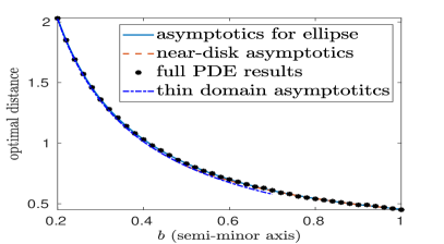
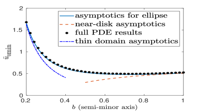
Figure 6: The optimal trap distance from the origin (left panel) and optimal average MFPT $\overline{u}_{0\mbox{min}}$ (right panel) versus the semi-minor axis $b$ of an elliptical domain of area $\pi$ that contains two traps of a common radius $\varepsilon=0.05$ and $D=1$. The optimum trap locations are on the semi-major axis, equidistant from the origin. Solid curves: hybrid asymptotic theory (4.32) for the ellipse coupled to the ODE relaxation scheme (4.33) to find the minimum. Dashed line (red): near-disk asymptotics of (2.26). Discrete points: full numerical PDE results computed from the closest point method. Dashed-dotted line (blue): thin-domain asymptotics (4.45). These curves essentially overlap with those from the hybrid theory for the optimal trap distance.

For $m=2$ traps, in the right panel of Fig. 6 we show results for the optimal average MFPT versus the semi-minor axis $b$ of the ellipse. The hybrid theory is seen to compare very favorably with full numerical PDE results for all $b\leq 1$. For $b$ near unity and for $b$ small, the near-disk theory of (2.26) and (3.30), and the thin-domain asymptotic result in (4.45) are seen to provide, respectively, good predictions for the optimal MFPT. Our hybrid theory shows that the optimal trap locations are on the semi-major axis for all $b<1$. In the left panel of Fig. 6, the optimal trap locations found from the steady-state of our ODE relaxation (4.33) are seen to compare very favorably with full PDE results. Remarkably, we observe that the thin-domain asymptotics prediction in (4.45) agrees well with the optimal locations from our hybrid theory for $b<0.7$.

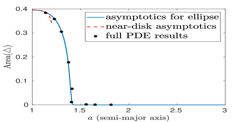
Figure 7: Area of the triangle formed by the three optimally located traps of a common radius $\varepsilon=0.05$ with $D=1$ in a deforming ellipse of area $\pi$ versus versus the semi-major axis $a$. The optimal traps become collinear as $a$ increases. Solid curve: hybrid asymptotic theory (4.32) for the ellipse coupled to the ODE relaxation scheme (4.33) to find the minimum. Dashed line: near-disk asymptotics of (2.26). Discrete points: full numerical PDE results computed from the closest point method.

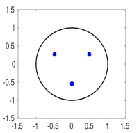
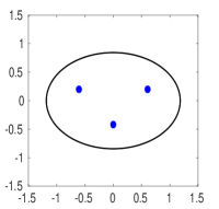
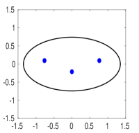
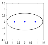
Figure 8: Optimal three-trap configurations for $D=1$ in a deforming ellipse of area $\pi$ with semi-major axis $a$ and a common trap radius $\varepsilon=0.05$. Left: $a=1$, $b=1$. Middle Left: $a=1.184$, $b\approx 0.845$. Middle Right: $a=1.351$, $b\approx 0.740$. Right: $a=1.450$, $b\approx 0.690$. The optimally located traps form an isosceles triangle as they deform from a ring pattern in the unit disk to a collinear pattern as $a$ increases.

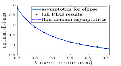
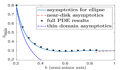
Figure 9: Left panel: Optimal distance from the origin for a collinear three-trap pattern on the major-axis of an ellipse of area $\pi$ versus the semi-minor axis $b$. When $b\leq 0.71$ the optimal pattern has a trap at the center and a pair of traps symmetrically located on either side of the origin. Right panel: optimal average MFPT $\overline{u}_{0\mbox{min}}$ versus $b$. Solid curves: hybrid asymptotic theory (4.32) for the ellipse coupled to the ODE relaxation scheme (4.33) to find the minimum. Dashed line (red): near-disk asymptotics of (2.26). Discrete points: Full PDE numerical results computed using the closest point method. Dashed-dotted line (blue): thin-domain asymptotics (4.48).

Next, we consider the case $m=3$. To clearly illustrate how the optimal trap configuration changes as the aspect ratio of the ellipse is varied, we use the hybrid theory to compute the area of the triangle formed by the three optimally located traps. The results shown in Fig. 7 are seen to compare favorably with full PDE results. These results show that that the optimal traps become colinear on the semi-major axis when $a\geq 1.45$. In Fig. 8 we show snapshots, at certain values of the semi-major axis, of the optimal trap locations in the ellipse. In the right panel of Fig. 9, we show that the optimal average MFPT from the hybrid theory compares very well with full numerical PDE results for all $b\leq 1$, and that the thin domain asymptotics (4.48) provides a good approximation when $b\leq 0.3$. In the left panel of Fig. 9 we plot the optimal trap locations on the semi-major axis when the trap pattern is collinear. We observe that results for the optimal trap locations from the hybrid theory, the thin domain asymptotics (4.48), and the full PDE simulations, essentially coincide on the full range $0.2<b<0.7$.

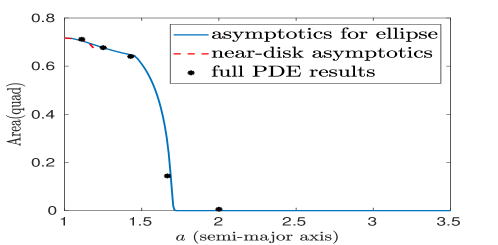
Figure 10: Area of the quadrilateral formed by the four optimally located traps of a common radius $\varepsilon=0.05$ with $D=1$ in a deforming ellipse of area $\pi$ and semi-major axis $a$. The optimal traps become collinear as $a$ increases. Solid curve: hybrid asymptotic theory (4.32) for the ellipse coupled to the ODE relaxation scheme (4.33) to find the minimum. Dashed line (red): near-disk asymptotics of (2.26). Discrete points: full numerical PDE results computed from the closest point method.

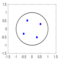
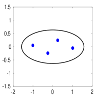
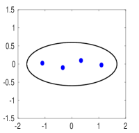
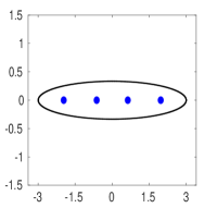
Figure 11: Optimal four-trap configurations for $D=1$ in a deforming ellipse of area $\pi$ with semi-major axis $a$ and a common trap radius $\varepsilon=0.05$. Left: $a=1$, $b=1$. Middle Left: $a=1.577$, $b\approx 0.634$. Middle Right: $a=1.675$, $b\approx 0.597$. Right: $a=3.0$, $b\approx 0.333$. The optimally located traps form a rectangle, followed by a parallelogram, as they deform from a ring pattern in the unit disk to a collinear pattern as $a$ increases.

For the case of four traps, where $m=4$, in Fig. 10 we use the hybrid theory to plot the area of the quadrilateral formed by the four optimally located traps versus the semi-major axis $a>1$. The full PDE results, also shown in Fig. 10, compare well with the hybrid results. This figure shows that as the aspect ratio of the ellipse increases the traps eventually become collinear on the semi-major axis when $a\geq 1.7$. This feature is further illustrated by the snapshots of the optimal trap locations shown in Fig. 11 at representative values of $a$. In the right panel of Fig. 12, we show that the hybrid and full numerical PDE results for the optimal average MFPT agree very closely for all $b\leq 1$, but that the thin-domain asymptotic result (4.51) agrees well only when $b\leq 0.25$. However, as similar to the three-trap case, on the range of $b$ where the trap pattern is collinear, in the left panel of Fig. 12 we show that the hybrid theory, the full PDE simulations, and the thin-domain asymptotics all provide essentially indistinguishable predictions for the optimal trap locations on the semi-major axis.

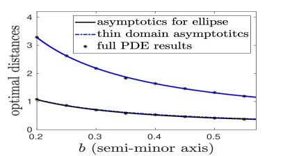
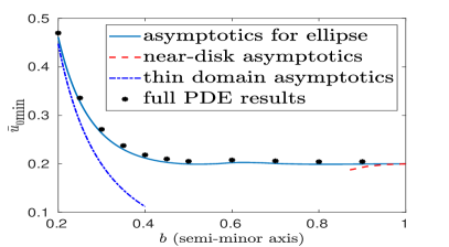
Figure 12: Left panel: Optimal distances from the origin for a collinear four-trap pattern on the major-axis of an ellipse of area $\pi$ and semi-minor axis $b$. When $b\leq 0.57$ the optimal pattern has two pairs of traps symmetrically located on either side of the origin. Right panel: the optimal average MFPT $\overline{u}_{0\mbox{min}}$ versus $b$. Solid curves: hybrid asymptotic theory (4.32) for the ellipse coupled to the ODE relaxation scheme (4.33) to find the minimum. Dashed line (red): near-disk asymptotics of (2.26). Discrete points: full numerical PDE results computed from the closest point method. Dashed-dotted line (blue): thin-domain asymptotics (4.51).

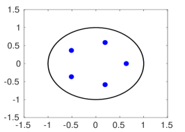
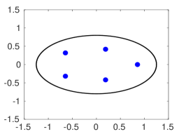
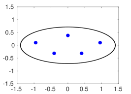
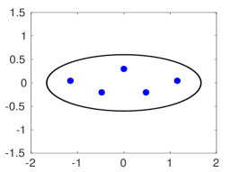
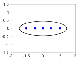
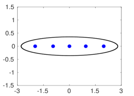
Figure 13: Optimal five-trap configurations for $D=1$ in a deforming ellipse of area $\pi$ with semi-major axis $a$ and a common trap radius $\varepsilon=0.05$. Top left: $a=1$, $b=1$. Top middle: $a=1.25$, $b=0.8$. Top right: $a=1.4$, $b\approx 0.690$. Bottom left: $a=1.665$, $b\approx 0.601$. Bottom middle: $a=2.22$, $b\approx 0.450$. Bottom right: $a=2.79$, $b\approx 0.358$. The optimal traps become collinear as $a$ increases and the edge-most traps become closer to the corner of the domain as $a$ increases.

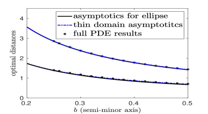
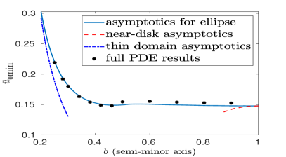
Figure 14: Left panel: Optimal distances from the origin for a collinear five-trap pattern on the major-axis of an ellipse of area $\pi$ and semi-minor axis $b$. When $b\leq 0.51$ the optimal pattern has a trap at the center and two pairs of traps symmetrically located on either side of the origin. Right panel: The optimal average MFPT $\overline{u}_{0\mbox{min}}$ versus $b$. Solid curves: hybrid asymptotic theory for the ellipse (4.32) coupled to the ODE relaxation scheme (4.33) to find the minimum. Dashed line (red): near-disk asymptotics of (2.26). Discrete points: full numerical PDE results computed from the closest point method. Dashed-dotted line (blue): thin-domain asymptotics (4.53).

Finally, we show similar results for the case of five traps. In Fig. 13, we plot the optimal trap locations in the ellipse as the semi-major axis of the ellipse is varied. This plot shows that the optimal pattern becomes collinear when (roughly) $a\geq 2$. In the right panel of Fig. 14, we show a close agreement between the hybrid and full numerical PDE results for the optimal average MFPT. However, as seen in Fig. 14, the thin-domain asymptotic result (4.53) accurately predicts the optimal MFPT only for rather small $b$. As for the four-trap case, in the left panel of Fig. 14 we show that the hybrid theory, the full PDE simulations, and the thin-domain asymptotics all yield similar predictions for the optimal trap locations on the semi-major axis.

4.2 Thin-Domain Asymptotics

For a long and thin ellipse, where $b=\delta\ll 1$ and $a={1/\delta}$ but with $|\Omega|=\pi$, we now derive simple approximations for the optimal trap locations and the optimal average MFPT using an approach based on thin-domain asymptotics. For $m=2$ the optimal trap locations are on the semi-major axis (cf. Fig. 6), while for $3\leq m\leq 5$ the optimal trap locations become collinear when the semi-minor axis $b$ decreases below a threshold (see Fig. 8, Fig. 11, and Fig. 13).

As derived in Appendix A, the leading-order approximation for the MFPT $u$ satisfying (2.2) in a thin elliptical with $b=\delta\ll 1$ is

(4.38) $$u(x,y)\sim\delta^{-2}U_{0}(\delta x)+{\mathcal{O}}(\delta^{-1})\,,$$

where the one-dimensional profile $U_{0}(X)$, with $x={X/\delta}$, satisfies the ODE

(4.39) $$\left[\sqrt{1-X^{2}}\,U_{0}^{\prime}\right]^{\prime}=-\frac{\sqrt{1-X^{2}}}{D}\,,\quad\mbox{on}\quad|X|\leq 1\,,$$

with $U_{0}$ and $U_{0}^{\prime}$ bounded as $X\to\pm 1$. In terms of $U_{0}(X)$, the average MFPT for the thin ellipse is estimated for $\delta\ll 1$ as

(4.40) $$\overline{u}_{0}\sim\frac{1}{\pi}\int_{-1/\delta}^{1/\delta}\int_{-\delta\sqrt{1-\delta^{2}x^{2}}}^{\delta\sqrt{1-\delta^{2}x^{2}}}u\,dxdy\sim\frac{4}{\pi\delta^{2}}\int_{0}^{1}\sqrt{1-X^{2}}\,U_{0}(X)\,dX\,.$$

In the thin domain limit, the circular traps of a common radius $\varepsilon$ centered on the semi-major axis are approximated by zero point constraints for $U_{0}$ at locations on the interval $|X|\leq 1$. In this way, (4.39) becomes a multi-point BVP problem, whose solution depends on the locations of the zero point constraints. Optimal values for the location of these constraints are obtained by minimizing the 1-D integral in (4.40) approximating $\overline{u}_{0}$. We now apply this approach for $m=2,\ldots,5$ collinear traps.

For $m=2$ traps centered at $X=\pm d$ with $0<d<1$, the multi-point BVP for $U_{0}(X)$ on $0<X<1$ satisfies

(4.41) $$\left[\sqrt{1-X^{2}}\,U_{0}^{\prime}\right]^{\prime}=-\frac{\sqrt{1-X^{2}}}{D}\,,\quad 0<X<1\,;\qquad U_{0}^{\prime}(0)=0\,,\quad U_{0}(d)=0\,,$$

with $U_{0}$ and $U_{0}^{\prime}$ bounded as $X\to\pm 1$. A particular solution for (4.41) is $U_{0p}=-{[(\sin^{-1}(X))^{2}+X^{2}]/(4D)}$, while the homogeneous solution is $U_{0H}=c_{1}\sin^{-1}(X)+c_{2}$. By combining these solutions, we readily calculate that

(4.42a) $$U_{0}(X)=\begin{cases}-\frac{1}{4D}\left[\left(\sin^{-1}{X}\right)^{2}+X^{2}-\pi\sin^{-1}X+c_{2}\right]\,,\quad d\leq X\leq 1\,,\\ -\frac{1}{4D}\left[\left(\sin^{-1}{X}\right)^{2}+X^{2}+c_{1}\right]\,,\quad 0\leq X\leq d\,,\end{cases}$$

where $$c_{1} c_{2}$$ and are given by

(4.42b) $$c_{1}=-d^{2}-\left(\sin^{-1}{d}\right)^{2}\,,\qquad c_{2}=-d^{2}+\pi\sin^{-1}{d}-\left(\sin^{-1}{d}\right)^{2}\,.$$

Upon substituting (4.42a) into (4.40), we obtain that

(4.43a) $$\overline{u}_{0}\sim-\frac{1}{\pi D\delta^{2}}\left[J_{0}+{\mathcal{H}}(d)\right]\,,$$

where the two integrals $$J_{0} {\mathcal{H}}(d)$$ and are given by

(4.43b) $$J_{0} \equiv\int_{0}^{1}F(X)\left[\left(\sin^{-1}{X}\right)^{2}+X^{2}-\pi\sin^{-1}(X)\right]\,dX\approx-0.703\,,$$

(4.43c) $${\mathcal{H}}(d) \equiv\pi\int_{0}^{d}F(X)\sin^{-1}(X)\,dX+c_{2}\int_{d}^{1}F(X)\,dX+c_{1}\int_{0}^{d}F(X)\,dX\,,$$

where $F(X)=\sqrt{1-X^{2}}$. By performing a few quadratures, and using (4.42b) for $c_{1}$ and $c_{2}$, we obtain an explicit expression for ${\mathcal{H}}(d)$:

(4.44) $${\mathcal{H}}(d)=-\frac{\pi}{2}\left[\sin^{-1}(d)\right]^{2}+\frac{\pi^{2}}{4}\sin^{-1}(d)-\frac{\pi d^{2}}{2}\,.$$

To estimate the optimal average MFPT we simply maximize ${\mathcal{H}}(d)$ in (4.44) on $0<d<1$. We compute that $d_{\textrm{opt}}\approx 0.406$, and correspondingly $\overline{u}_{0\mbox{min}}=-\left(\pi D\delta^{2}\right)^{-1}\left[J_{0}+{\mathcal{H}}(d_{\textrm{opt}})\right]$. Then, by setting $\delta=b$ and $x_{\textrm{opt}}={d_{\textrm{opt}}/\delta}$, we obtain the following estimate for the optimal trap location and minimum average MFPT for $m=2$ traps in the thin domain limit:

(4.45) $$x_{0\textrm{opt}}\sim{0.406/b}\,,\qquad\overline{u}_{0\textrm{opt}}\sim{0.0652/(b^{2}D)}\,,\quad\mbox{for}\quad b\ll 1\,.$$

These estimates are favorably compared in Fig. 6 with full PDE solutions computed using the closest point method [10] and with the full asymptotic theory based on (4.32).

Next, suppose that $m=3$. Since there is an additional trap at the origin, we simply replace the condition $U_{0}^{\prime}(0)=0$ in (4.41) with $U_{0}(0)=0$. In place of (4.42a),

(4.46a) $$U_{0}(X)=\begin{cases}-\frac{1}{4D}\left[\left(\sin^{-1}{X}\right)^{2}+X^{2}-\pi\sin^{-1}X+c_{2}\right]\,,\quad d\leq X\leq 1\,,\\ -\frac{1}{4D}\left[\left(\sin^{-1}{X}\right)^{2}+X^{2}+c_{1}\sin^{-1}{X}\right]\,,\quad 0\leq X\leq d\,,\end{cases}$$

where $$c_{1} c_{2}$$ and are given by

(4.46b) $$c_{1}=-{\left(d^{2}+\left[\sin^{-1}(d)\right]^{2}\right)/\sin^{-1}(d)}\,,\qquad c_{2}=-d^{2}+\pi\sin^{-1}(d)-\left[\sin^{-1}(d)\right]^{2}\,.$$

The average MFPT is given by (4.43a), where ${\mathcal{H}}(d)$ is now defined by

(4.47) $${\mathcal{H}}(d)\equiv c_{2}\int_{d}^{1}F(X)\,dX+(c_{1}+\pi)\int_{0}^{d}F(X)\,\sin^{-1}(X)\,dX\,,$$

with $F(X)=\sqrt{1-X^{2}}$. By maximizing ${\mathcal{H}}(d)$ on $0<d<1$, we obtain $d_{\textrm{opt}}\approx 0.567$, so that $\overline{u}_{0\mbox{min}}=-\left(\pi D\delta^{2}\right)^{-1}\left[J_{0}+{\mathcal{H}}(d_{\textrm{opt}})\right]$. In this way, the optimal trap location and the minimum of the average MFPT satisfies

(4.48) $$x_{0\textrm{opt}}\sim{0.567/b}\,,\qquad\overline{u}_{0\textrm{opt}}\sim{0.0308/(b^{2}D)}\,,\quad\mbox{for}\quad b\ll 1\,.$$

In Fig. 9 these scaling laws are seen to compare well with full PDE solutions and with the full asymptotic theory of (4.32), even when $b$ is only moderately small.

Next, we consider the case $m=4$, with two symmetrically placed traps on either side of the origin. Therefore, we solve (4.41) with $U_{0}^{\prime}(0)=0$, $U_{0}(d_{1})=0$, and $U_{0}(d_{2})=0$, where $0<d_{1}<d_{2}$. In place of (4.42a), we get

(4.49a) $$U_{0}(X)=\begin{cases}-\frac{1}{4D}\left[\left(\sin^{-1}{X}\right)^{2}+X^{2}-\pi\sin^{-1}X+c_{2}\right]\,,\quad d_{2}\leq X\leq 1\,,\\ -\frac{1}{4D}\left[\left(\sin^{-1}{X}\right)^{2}+X^{2}+b_{1}\sin^{-1}{X}+b_{2}\right]\,,\quad d_{1}\leq X\leq d_{2}\,,\\ -\frac{1}{4D}\left[\left(\sin^{-1}{X}\right)^{2}+X^{2}+c_{1}\right]\,,\quad 0\leq X\leq d_{1}\,,\end{cases}$$

where $$c_{1} c_{2}$$ and are given by

(4.49b) $$\begin{split}&\qquad\qquad\qquad c_{1}=-d_{1}^{2}-\left(\sin^{-1}{d_{1}}\right)^{2}\,,\qquad c_{2}=-d_{2}^{2}+\pi\sin^{-1}{d_{2}}-\left(\sin^{-1}{d_{2}}\right)^{2}\,,\\ b_{1}&=\frac{\left(\sin^{-1}{d_{1}}\right)^{2}-\left(\sin^{-1}{d_{2}}\right)^{2}+d_{1}^{2}-d_{2}^{2}}{\sin^{-1}{d_{2}}-\sin^{-1}{d_{1}}}\,,\qquad b_{2}=-b_{1}\sin^{-1}d_{1}-d_{1}^{2}-\left(\sin^{-1}{d_{1}}\right)^{2}\,.\end{split}$$

The average MFPT is given by (4.43a), where ${\mathcal{H}}={\mathcal{H}}(d_{1},d_{2})$ is now given by

(4.50) $$\begin{split}{\mathcal{H}}(d_{1},d_{2})&\equiv c_{2}\int_{d_{2}}^{1}F(X)\,dX+(b_{1}+\pi)\int_{d_{1}}^{d_{2}}F(X)\,\sin^{-1}(X)\,dX+b_{2}\int_{d_{1}}^{d_{2}}F(X)\,dX\\ &\qquad+\pi\int_{0}^{d_{1}}F(X)\,\sin^{-1}(X)\,dX+c_{1}\int_{0}^{d_{1}}F(X)\,dX\,,\end{split}$$

where $F(X)\equiv\sqrt{1-X^{2}}$. By using a grid search to maximize ${\mathcal{H}}(d_{1},d_{2})$ on $0<d_{1}<d_{2}<1$, we obtain that $d_{1\textrm{opt}}\approx 0.215$ and $d_{2\textrm{opt}}\approx 0.656$. This yields that the optimal trap locations and the minimum of the average MFPT, given by $\overline{u}_{0\mbox{min}}=-\left(\pi D\delta^{2}\right)^{-1}\left[J_{0}+{\mathcal{H}}(d_{1\textrm{opt}},d_{2\textrm{opt}})\right]$, have the scaling law

(4.51) $$x_{1\textrm{opt}}\sim{0.215/b}\,,\quad x_{2\textrm{opt}}\sim{0.656/b}\,,\quad\overline{u}_{0\textrm{opt}}\sim{0.0179/(b^{2}D)}\,,\quad\mbox{for}\quad b\ll 1\,.$$

These scaling laws are shown in Fig. 12 to agree well with the full PDE solutions and with the full asymptotic theory of (4.32) when $b$ is small.

Finally, we consider the case $m=5$, where we need only modify the $m=4$ analysis by adding a trap at the origin. Setting $U_{0}(0)=0$, $U_{0}(d_{1})=0$, and $U_{0}(d_{2})=0$ we obtain that $U_{0}$ is again given by (4.49a), except that now $c_{1}$ in (4.49a) is replaced by $c_{1}\sin^{-1}(X)$, with $c_{1}$ as defined in (4.46b). The average MFPT satisfies (4.43a), where in place of (4.50) we obtain that ${\mathcal{H}}(d_{1},d_{2})$ is given by

(4.52) $$\begin{split}{\mathcal{H}}(d_{1},d_{2})&\equiv c_{2}\int_{d_{1}}^{1}F(X)\,dX+(b_{1}+\pi)\int_{d_{1}}^{d_{2}}F(X)\,\sin^{-1}(X)\,dX\\ &\qquad+b_{2}\int_{d_{1}}^{d_{2}}F(X)\,dX+(c_{1}+\pi)\int_{0}^{d_{1}}F(X)\,\sin^{-1}{X}\,dX\,,\end{split}$$

with $F(X)=\sqrt{1-X^{2}}$. A grid search yields that ${\mathcal{H}}(d_{1},d_{2})$ is maximized on $0<d_{1}<d_{2}<1$ when $d_{1\textrm{opt}}\approx 0.348$ and $d_{2\textrm{opt}}\approx 0.714$. In this way, the corresponding optimal trap locations and minimum average MFPT have the scaling law

(4.53) $$x_{1\textrm{opt}}\sim{0.348/b}\,,\quad x_{2\textrm{opt}}\sim{0.714/b}\,,\quad\overline{u}_{0\textrm{opt}}\sim{0.0117/(b^{2}D)}\,,\quad\mbox{for}\quad b\ll 1\,.$$

Fig. 14 shows that (4.53) compares well with the full PDE solutions and with the full asymptotic theory of (4.32) when $b$ is small.

5 An Explicit Neumann Green’s Function for the Ellipse

We derive the new explicit formula (4.36) for the Neumann Green’s function and its regular part in (4.37) in terms of rapidly converging infinite series. This Green’s function $G(\mathbf{x};\mathbf{x}_{0})$ for the ellipse $\Omega\equiv\{{\mathbf{x}=(x,y)\,|\,{x^{2}/a^{2}}+{y^{2}/b^{2}}\leq 1\}}$ is the unique solution to

(5.54a) $$\Delta G =\frac{1}{|\Omega|}-\delta(\mathbf{x}-\mathbf{x}_{0})\,\quad\mathbf{x}\in\Omega\,;\qquad\partial_{n}G=0\,,\,\,\,\mathbf{x}\in\partial\Omega\,;$$

(5.54b) $$G\sim-\frac{1}{2\pi} \log{|\mathbf{x}-\mathbf{x}_{0}|}+R_{e}+o(1)\quad\text{as}\quad\mathbf{x}\to\mathbf{x}_{0}\,;\qquad\int_{\Omega}G\,\text{d}\mathbf{x}=0\,,$$

where $|\Omega|=\pi ab$ is the area of $\Omega$ and $R_{e}$ is the regular part of the Green’s function. Here $\partial_{n}G$ is the outward normal derivative to the boundary of the ellipse. To remove the $|\Omega|^{-1}$ term in (5.54a), we introduce $N(\mathbf{x};\mathbf{x}_{0})$ defined by

(5.55) $$G(\mathbf{x};\mathbf{x}_{0})=\frac{1}{4|\Omega|}(x^{2}+y^{2})+N(\mathbf{x};\mathbf{x}_{0})\,.$$

We readily derive that $N(\mathbf{x};\mathbf{x}_{0})$ satisfies

(5.56a) $$\Delta N =-\delta(\mathbf{x}-\mathbf{x}_{0})\quad\mathbf{x}\in\Omega\,;\quad\partial_{n}N=-\frac{1}{2|\Omega|\sqrt{{x^{2}/a^{4}}+{y^{2}/b^{4}}}}\,,\,\,\,\mathbf{x}\in\partial\Omega\,;$$

(5.56b) $$\int_{\Omega}N\,\text{d}\mathbf{x} =-\frac{1}{4|\Omega|}\int_{\Omega}(x^{2}+y^{2})\,\text{d}\mathbf{x}=-\frac{1}{4|\Omega|}\left(\frac{|\Omega|}{4}(a^{2}+b^{2})\right)=-\frac{1}{16}(a^{2}+b^{2})\,.$$

We assume that $a>b$, so that the semi-major axis is on the $x$-axis. To solve (5.56) we introduce the elliptic cylindrical coordinates $(\xi,\eta)$ defined by (4.34) and its inverse mapping (4.35). We set $\mathcal{N}(\xi,\eta)\equiv N(x(\xi,\eta),y(\xi,\eta))$ and seek to convert (5.56) to a problem for $\mathcal{N}$ defined in a rectangular domain. It is well-known that

(5.57) $$N_{xx}+N_{yy}=\frac{1}{f^{2}(\cosh^{2}\xi-\cos^{2}\eta)}\left(\mathcal{N}_{\xi\xi}+\mathcal{N}_{\eta\eta}\right)\,.$$

Moreover, by computing the scale factors $h_{\xi}=\sqrt{x_{\xi}^{2}+y_{\xi}^{2}}$ and $h_{\eta}=\sqrt{x_{\eta}^{2}+y_{\eta}^{2}}$ of the transformation, we obtain that

(5.58) $$\delta(x-x_{0})\delta(y-y_{0})=\frac{1}{h_{\eta}h_{\xi}}\delta(\xi-\xi_{0})\delta(\eta-\eta_{0})=\frac{1}{f^{2}(\cosh^{2}\xi-\cos^{2}\eta)}\delta(\xi-\xi_{0})\delta(\eta-\eta_{0})\,,$$

where we used $h_{\xi}=h_{\eta}=f\sqrt{\cosh^{2}\xi_{0}-\cos^{2}\eta_{0}}$. By using (5.57) and (5.58), we obtain that the PDE in (5.56a) transforms to

(5.59) $$\mathcal{N}_{\xi\xi}+\mathcal{N}_{\eta\eta}=-\delta(\xi-\xi_{0})\delta(\eta-\eta_{0})\,,\quad\mbox{in}\quad 0\leq\eta\leq 2\pi\,,\,\,0\leq\xi\leq u_{b}\,.$$

To determine how the normal derivative in (5.56a) transforms, we calculate

(5.60) $$\begin{pmatrix}N_{x}\\ N_{y}\end{pmatrix}=\frac{1}{x_{\xi}y_{\eta}-x_{\eta}y_{\xi}}\begin{pmatrix}y_{\eta}&-y_{\xi}\\ -x_{\eta}&x_{\xi}\end{pmatrix}\begin{pmatrix}\mathcal{N}_{\xi}\\ \mathcal{N}_{\eta}\end{pmatrix}\,,$$

where from (4.34a) we calculate

(5.61) $$x_{\xi}=f\sinh\xi\cos\eta=y_{\eta}\,,\qquad x_{\eta}=-f\cosh\xi\sin\eta=-y_{\xi}\,.$$

Now using $x=a\cos\eta$ and $y=b\sin\eta$ on $\partial\Omega$, we calculate on $\partial\Omega$ that

(5.62) $$\partial_{n}N=\nabla N\cdot\frac{(x/a^{2}\,,y/b^{2})}{\sqrt{x^{2}/a^{4}+y^{2}/b^{4}}}=\frac{\left(\frac{1}{a}\cos\eta\,\,,\frac{1}{b}\sin\eta\right)}{\sqrt{x^{2}/a^{4}+y^{2}/b^{4}}\left(x_{\xi}y_{\eta}-x_{\eta}y_{\xi}\right)}\begin{pmatrix}y_{\eta}&-y_{\xi}\\ -x_{\eta}&x_{\xi}\end{pmatrix}\begin{pmatrix}\mathcal{N}_{\xi}\\ \mathcal{N}_{\eta}\end{pmatrix}.$$

By using (5.61), we calculate on $\partial\Omega$ that $x_{\xi}y_{\eta}-x_{\eta}y_{\xi}=b^{2}\cos^{2}\eta+a^{2}\sin^{2}\eta$. With this expression, we obtain after some algebra that (5.62) becomes

(5.63) $$\partial_{n}N=\frac{1}{ab\sqrt{x^{2}/a^{4}+y^{2}/b^{4}}}\,\mathcal{N}_{u}\,,\quad\mbox{on}\quad\xi=\xi_{b}\,.$$

By combining (5.63) and (5.56a), we obtain $\mathcal{N}_{\xi}=-{1/(2\pi)}$ on $\xi=\xi_{b}$.

Next, we discuss the other boundary conditions in the transformed plane. We require that $\mathcal{N}$ and $\mathcal{N}_{\eta}$ are $2\pi$ periodic in $\eta$. The boundary condition imposed on $\eta=0$, which corresponds to the line segment $y=0$ and $|x|\leq f=\sqrt{a^{2}-b^{2}}$ between the two foci, is chosen to ensure that $N$ and the normal derivative $N_{y}$ are continuous across this segment. Recall from (4.35b) that the top of this segment $y=0^{+}$ and $|x|\leq f$ corresponds to $0\leq\eta\leq\pi$, while the bottom of this segment $y=0^{-}$ and $|x|\leq f$ corresponds to $\pi\leq\eta\leq 2\pi$. To ensure that $N$ is continuous across this segment, we require that $\mathcal{N}(\xi,\eta)$ satisfies $\mathcal{N}(0,\eta)=\mathcal{N}(0,2\pi-\eta)$ for any $0\leq\eta\leq\pi$. Moreover, since $\mathcal{N}_{\xi}=N_{y}f\sin\eta$ on $\xi=0$, and $\sin(2\pi-\eta)=-\sin(\eta)$, we must have $\mathcal{N}_{\xi}(0,\eta)=\mathcal{N}_{\xi}(0,2\pi-\eta)$ on $0\leq\eta\leq\pi$.

Finally, we examine the normalization condition in (5.56b) by using

(5.64) $$\int_{\Omega}N(x,y)\,dx\,dy=\int_{0}^{\xi_{b}}\int_{0}^{2\pi}\mathcal{N}(\xi,\eta)\,\,\Big{|}\mbox{det}\begin{pmatrix}x_{\xi}&x_{\eta}\\ y_{\xi}&y_{\eta}\end{pmatrix}\Big{|}\,d\xi\,d\eta\,.$$

Since $x_{\xi}y_{\eta}-x_{\eta}y_{\xi}=f^{2}\left(\cosh^{2}\xi-\cos^{2}\eta\right)$, we obtain from (5.64) that (5.56b) becomes

(5.65) $$\int_{0}^{\xi_{b}}\int_{0}^{2\pi}\mathcal{N}(\xi,\eta)\left[\cosh^{2}\xi-\cos^{2}\eta\right]\,d\xi\,d\eta=-\frac{1}{16f^{2}}{(a^{2}+b^{2})}=-\frac{(a^{2}+b^{2})}{16(a^{2}-b^{2})}\,.$$

In summary, from (5.59), (5.65), and the condition on $\xi=\xi_{b}$, $\mathcal{N}(\xi,\eta)$ satisfies

(5.66a) $$\Delta\mathcal{N}=-\delta(\xi-\xi_{0})\delta(\eta-\eta_{0})\,\quad 0\leq\xi\leq\xi_{b}\,,\,\,0\leq\eta\leq\pi\,,$$

(5.66b) $$\partial_{\xi}\mathcal{N}=-\frac{1}{2\pi}\,,\quad\mbox{on}\,\,\xi=\xi_{b}\,;\qquad\mathcal{N}\,,\,\,\mathcal{N}_{\eta}\quad 2\pi\,\,\mbox{periodic in }\eta\,,$$

(5.66c) $$\mathcal{N}(0,\eta)=\mathcal{N}(0,2\pi-\eta)\,,\quad\mathcal{N}_{\xi}(0,\eta)=-\mathcal{N}_{\xi}(0,2\pi-\eta)\,,\quad\mbox{for}\quad 0\leq\eta\leq\pi\,,$$

(5.66d) $$\int_{0}^{\xi_{b}}\int_{0}^{2\pi}\mathcal{N}(\xi,\eta)\left[\cosh^{2}\xi-\cos^{2}\eta\right]\,d\xi\,d\eta=-\frac{(a^{2}+b^{2})}{16(a^{2}-b^{2})}\,.$$

The solution to (5.66) is expanded in terms of the eigenfunctions in the $\eta$ direction:

(5.67) $$\mathcal{N}(\xi,\eta)=\mathcal{A}_{0}(\xi)+\sum_{k=1}^{\infty}\mathcal{A}_{k}(\xi)\cos(k\eta)+\sum_{k=1}^{\infty}\mathcal{B}_{k}(\xi)\sin(k\eta)\,.$$

The boundary condition (5.66b) is satisfied with $\mathcal{A}_{0}^{\prime}(\xi_{b})=-{1/(2\pi)}$ and $\mathcal{A}_{k}^{\prime}(\xi_{b})=\mathcal{B}_{k}^{\prime}(\xi_{b})=0$, for $k\geq 1$. To satisfy $\mathcal{N}(0,\eta)=\mathcal{N}(0,2\pi-\eta)$, we require $\mathcal{B}_{k}(0)=0$ for $k\geq 1$. Finally, to satisfy $\mathcal{N}_{\xi}(0,\eta)=-\mathcal{N}_{\xi}(0,2\pi-\eta)$, we require that $\mathcal{A}_{0}^{\prime}(0)=0$ and $\mathcal{A}_{k}^{\prime}(0)=0$ for $k\geq 1$. In the usual way, we can derive ODE boundary value problems for $\mathcal{A}_{0}$, $\mathcal{A}_{k}$, and $\mathcal{B}_{k}$. We obtain that

(5.68a) $$\mathcal{A}_{0}^{\prime\prime}=-\frac{1}{2\pi}\delta(\xi-\xi_{0})\,,\quad 0\leq\xi\leq\xi_{b}\,;\qquad\mathcal{A}_{0}^{\prime}(0)=0\,,\,\,\,\mathcal{A}_{0}^{\prime}(\xi_{b})=-\frac{1}{2\pi}\,,$$

while on $$0\leq\xi\leq\xi_{b} k=1,2,\ldots$$, and for each , we have

(5.68b) $$\mathcal{A}_{k}^{\prime\prime}-k^{2}\mathcal{A}_{k}=-\frac{1}{\pi}\cos(k\eta_{0})\delta(\xi-\xi_{0})\,;\qquad\mathcal{A}_{k}^{\prime}(0)=0\,,\,\,\,\mathcal{A}_{k}^{\prime}(\xi_{b})=0\,,$$

(5.68c) $$\mathcal{B}_{k}^{\prime\prime}-k^{2}\mathcal{B}_{k}=-\frac{1}{\pi}\sin(k\eta_{0})\delta(\xi-\xi_{0})\,;\qquad\mathcal{B}_{k}(0)=0\,,\,\,\,\mathcal{B}_{k}^{\prime}(\xi_{b})=0\,.$$

We observe from (5.68a) that $\mathcal{A}_{0}$ is specified only up to an arbitrary constant.

We determine this constant from the normalization condition (5.66d). By substituting (5.67) into (5.66d), we readily derive the identity that

(5.69) $$\int_{0}^{\xi_{b}}\mathcal{A}_{0}(\xi)\cosh(2\xi)\,d\xi-\frac{1}{2}\int_{0}^{\xi_{b}}\mathcal{A}_{2}(\xi)\,d\xi=-\frac{1}{16\pi}\left(\frac{a^{2}+b^{2}}{a^{2}-b^{2}}\right)\,.$$

We will use (5.69) to derive a point constraint on $\mathcal{A}_{0}(\xi_{b})$. To do so, we define $\phi(\xi)=\cosh(2\xi)$, which satisfies $\phi^{\prime\prime}-4\phi=0$ and $\phi^{\prime}(0)=0$. We integrate by parts and use $\mathcal{A}_{0}^{\prime}(0)=0$ and $\mathcal{A}_{0}^{\prime}(\xi_{b})=-{1/(2\pi)}$ to get

(5.70) $$\begin{split}4\int_{0}^{\xi_{b}}\mathcal{A}_{0}\phi\,d\xi=\int_{0}^{\xi_{b}}\mathcal{A}_{0}\phi^{\prime\prime}\,d\xi&=\left(\phi^{\prime}\mathcal{A}_{0}-\phi\mathcal{A}^{\prime}_{0}\right)|_{0}^{\xi_{b}}+\int_{0}^{\xi_{b}}\phi\mathcal{A}_{0}^{\prime\prime}\,d\xi\,,\\ &=\phi^{\prime}(\xi_{b})\mathcal{A}_{0}(\xi_{b})+\frac{1}{2\pi}\left[\phi(\xi_{b})-\phi(\xi_{0})\right]\,.\end{split}$$

Next, set $k=2$ in (5.68b) and integrate over $0<\xi<\xi_{b}$. Using the no-flux boundary conditions we get $\int_{0}^{\xi_{b}}\mathcal{A}_{2}\,d\xi={\cos(2\eta_{0})/(4\pi)}$. We substitute this result, together with (5.70), into (5.69) and solve the resulting equation for $\mathcal{A}_{0}(\xi_{b})$ to get

(5.71) $$\mathcal{A}_{0}(\xi_{b})=\frac{1}{4\pi\sinh(2\xi_{b})}\left[\cosh(2\xi_{0})+\cos(2\eta_{0})-\cosh(2\xi_{b})-\frac{1}{2}\left(\frac{a^{2}+b^{2}}{a^{2}-b^{2}}\right)\right]\,.$$

To simplify this expression we use $\tanh\xi_{b}={b/a}$ to calculate $\sinh(2\xi_{b})={2ab/(a^{2}-b^{2})}$ and $\coth(2\xi_{b})={(a^{2}+b^{2})/(2ab)}$, while from (4.34a) we get

$$x_{0}^{2}+y_{0}^{2}=f^{2}\left[\cosh^{2}\xi_{0}-\sin^{2}\eta_{0}\right]=\frac{(a^{2}-b^{2})}{2}\left[\cosh(2\xi_{0})+\cos(2\eta_{0})\right]\,.$$

Upon substituting these results into (5.71), we conclude that

(5.72) $$\mathcal{A}_{0}(\xi_{b})=-\frac{3}{16|\Omega|}(a^{2}+b^{2})+\frac{1}{4|\Omega|}\left(x_{0}^{2}+y_{0}^{2}\right)\,,$$

where $|\Omega|=\pi ab$ is the area of the ellipse. With this explicit value for $\mathcal{A}_{0}(\xi_{b})$, the normalization condition (5.66d), or equivalently the constraint $\int_{\Omega}G\,\text{d}\mathbf{x}=0$, is satisfied.

Next, we solve the ODEs (5.68) for $\mathcal{A}_{0}$, $\mathcal{A}_{k}$, and $\mathcal{B}_{k}$, for $k\geq 1$, to obtain

(5.73a) $$\mathcal{A}_{0}(\xi)=\frac{1}{2\pi}\left(\xi_{b}-\xi_{>}\right)+\mathcal{A}_{0}(\xi_{b})\,,\quad\mathcal{A}_{k}(\xi)=\frac{\cos(k\eta_{0})}{k\pi\sinh(k\xi_{b})}\cosh(k\xi_{<})\cosh\left(k(\xi_{>}-\xi_{b})\right)\,,$$

(5.73b) $$\mathcal{B}_{k}(\xi)=\frac{\sin(k\eta_{0})}{k\pi\cosh(k\xi_{b})}\sinh(k\xi_{<})\cosh\left(k(\xi_{>}-\xi_{b})\right)\,,$$

where we have defined $\xi_{>}\equiv\max(\xi_{0},\xi)$ and $\xi_{<}\equiv\min(\xi_{0},\xi)$.

To determine an explicit expression for $G(\mathbf{x};\mathbf{x}_{0})={|\mathbf{x}|^{2}/(4|\Omega|)}+\mathcal{N}(\xi,\eta)$, as given in (5.55), we substitute (5.72) and (5.73) into the eigenfunction expansion (5.67) for $\mathcal{N}$. In this way, we get

(5.74a) $$G(\mathbf{x};\mathbf{x}_{0})=\frac{1}{4|\Omega|}\left(|\mathbf{x}|^{2}+|\mathbf{x}_{0}|^{2}\right)-\frac{3}{16|\Omega|}(a^{2}+b^{2})+\frac{1}{2\pi}\left(\xi_{b}-\xi_{>}\right)+\mathcal{S}\,,$$

where the infinite sum $$\mathcal{S}$$ is defined by

(5.74b) $$\begin{split}\mathcal{S}&\equiv\sum_{k=1}^{\infty}\frac{\cos(k\eta_{0})\cos(k\eta)}{\pi k\sinh(k\xi_{b})}\cosh(k\xi_{<})\cosh\left(k(\xi_{>}-\xi_{b})\right)\\ &\qquad+\sum_{k=1}^{\infty}\frac{\sin(k\eta_{0})\sin(k\eta)}{\pi k\cosh(k\xi_{b})}\sinh(k\xi_{<})\cosh\left(k(\xi_{>}-\xi_{b})\right)\,.\end{split}$$

Next, from the product to sum formulas for $\cos(A)\cos(B)$ and $\sin(A)\sin(B)$ we get

(5.75) $$\begin{split}\mathcal{S}&=\frac{1}{2\pi}\sum_{k=1}^{\infty}\frac{\cosh\left(k(\xi_{>}-\xi_{b})\right)}{k}\left[\frac{\cosh(k\xi_{<})}{\sinh(k\xi_{b})}+\frac{\sin(k\xi_{<})}{\cosh(k\xi_{b})}\right]\cos\left(k(\eta-\eta_{0}\right)\\ &\qquad+\frac{1}{2\pi}\sum_{k=1}^{\infty}\frac{\cosh\left(k(\xi_{>}-\xi_{b})\right)}{k}\left[\frac{\cosh(k\xi_{<})}{\sinh(k\xi_{b})}-\frac{\sin(k\xi_{<})}{\cosh(k\xi_{b})}\right]\cos\left(k(\eta+\eta_{0}\right)\,.\end{split}$$

Then, by using product to sum formulas for $\cosh(A)\cosh(B)$, the identity $\sinh(2A)=2\sinh(A)\cosh(A)$, $\xi_{>}+\xi_{<}=\xi+\xi_{0}$, and $\xi_{>}-\xi_{<}=|\xi-\xi_{0}|$, some algebra yields that

(5.76) $$\begin{split}\mathcal{S}&=\frac{1}{2\pi}\mbox{Re}\left(\sum_{k=1}^{\infty}\frac{\left[\cosh\left(k(\xi+\xi_{0})\right)+\cosh\left(k(|\xi-\xi_{0}|-2\xi_{b})\right)\right]}{k\sinh(2k\xi_{b})}e^{ik(\eta-\eta_{0})}\right)\\ &\quad+\frac{1}{2\pi}\mbox{Re}\left(\sum_{k=1}^{\infty}\frac{\left[\cosh\left(k(\xi+\xi_{0}-2\xi_{b})\right)+\cosh\left(k|\xi-\xi_{0}|\right)\right]}{k\sinh(2k\xi_{b})}e^{ik(\eta+\eta_{0})}\right)\,.\end{split}$$

The next step in the analysis is to convert the hyperbolic functions in (5.76) into pure exponentials. A simple calculation yields that

(5.77a) $$\mathcal{S}=\frac{1}{2\pi}\mbox{Re}\left(\sum_{k=1}^{\infty}\frac{\mathcal{H}_{1}}{k}e^{ik(\eta-\eta_{0})}+\sum_{k=1}^{\infty}\frac{\mathcal{H}_{2}}{k}e^{ik(\eta+\eta_{0})}\right)\,,$$

where $$\mathcal{H}_{1} \mathcal{H}_{2}$$ and are defined by

(5.77b) $$\begin{split}\mathcal{H}_{1}&\equiv\frac{1}{1-e^{-4k\xi_{b}}}\left[e^{k(\xi+\xi_{0}-2\xi_{b})}+e^{-k(\xi+\xi_{0}+2\xi_{b})}+e^{k(|\xi-\xi_{0}|-4\xi_{b})}+e^{-k|\xi-\xi_{0}|}\right]\,,\\ \mathcal{H}_{2}&\equiv\frac{1}{1-e^{-4k\xi_{b}}}\left[e^{k(\xi+\xi_{0}-4\xi_{b})}+e^{k(|\xi-\xi_{0}|-2\xi_{b})}+e^{-k(|\xi-\xi_{0}|+2\xi_{b})}+e^{-k(\xi+\xi_{0})}\right]\,.\end{split}$$

Then, for any $q$ with $0<q<1$ and integer $k\geq 1$, we use the identity $\sum_{n=0}^{\infty}\left(q^{k}\right)^{n}=\frac{1}{1-q^{k}}$ for the choice $q=e^{-4\xi_{b}}$, which converts $\mathcal{H}_{1}$ and $\mathcal{H}_{2}$ into infinite sums. This leads to a doubly-infinite sum representation for $\mathcal{S}$ in (5.77a) given by

(5.78) $$\mathcal{S}=\frac{1}{2\pi}\mbox{Re}\left(\sum_{k=1}^{\infty}\sum_{n=0}^{\infty}\frac{\left(q^{n}\right)^{k}}{k}\left(z_{1}^{k}+z_{2}^{k}+z_{3}^{k}+z_{4}^{k}+z_{5}^{k}+z_{6}^{k}+z_{7}^{k}+z_{8}^{k}\right)\right)\,,$$

where the complex constants $z_{1},\ldots,z_{8}$ are defined by (4.36b). From these formulae, we readily observe that $|z_{j}|<1$ on $0\leq\xi\leq\xi_{b}$ for any $(\xi,\eta)\neq(\xi_{0},\eta_{0})$. Since $0<q<1$, we can then switch the order of the sums in (5.78) when $(\xi,\eta)\neq(\xi_{0},\eta_{0})$ and use the identity $\mbox{Re}\left(\sum_{k=1}^{\infty}k^{-1}\omega^{k}\right)=-\log|1-\omega|$, where $|1-\omega|$ denotes modulus. In this way, upon setting $\omega_{j}=q^{n}z_{j}$ for $j=1,\ldots,8$, we obtain a compact representation for $\mathcal{S}$. Finally, by using this result in (5.74) we obtain for $(\xi,\eta)\neq(\xi_{0},\eta_{0})$, or equivalently $(x,y)\neq(x_{0},y_{0})$, the result given explicitly in (4.36) of § 4.

Next, to determine the regular part of the Neumann Green’s function we must identify the singular term in (4.36a) at $(\xi,\eta)=(\xi_{0},\eta_{0})$. Since $z_{1}=1$, while $|z_{j}|<1$ for $j=2,\ldots,8$, at $(\xi,\eta)=(\xi_{0},\eta_{0})$, the singular contribution arises only from the $n=0$ term in $\sum_{n=0}^{\infty}\log|1-\beta^{2n}z_{1}|$. As such, we add and subtract the fundamental singularity $-{\log|\mathbf{x}-\mathbf{x}_{0}|/(2\pi)}$ in (4.36a) to get

(5.79a) $$G(\mathbf{x};\mathbf{x}_{0})=-\frac{1}{2\pi}\log|\mathbf{x}-\mathbf{x}_{0}|+R(\mathbf{x};\mathbf{x}_{0})\,,$$

(5.79b) $$\begin{split}R(\mathbf{x};\mathbf{x}_{0})&=\frac{1}{4|\Omega|}\left(|\mathbf{x}|^{2}+|\mathbf{x}_{0}|^{2}\right)-\frac{3(a^{2}+b^{2})}{16|\Omega|}-\frac{1}{4\pi}\log\beta-\frac{1}{2\pi}\xi_{>}+\frac{1}{2\pi}\log\left(\frac{|\mathbf{x}-\mathbf{x}_{0}|}{|1-z_{1}|}\right)\\ &\qquad-\frac{1}{2\pi}\sum_{n=1}^{\infty}\log|1-\beta^{2n}z_{1}|-\frac{1}{2\pi}\sum_{n=0}^{\infty}\log\left(\displaystyle\prod_{j=2}^{8}|1-\beta^{2n}z_{j}|\right)\,.\end{split}$$

To identify $\lim_{\mathbf{x}\to\mathbf{x}_{0}}R(\mathbf{x};\mathbf{x}_{0})=R_{e}$, we must find $\lim_{\mathbf{x}\to\mathbf{x}_{0}}\log\left({|\mathbf{x}-\mathbf{x}_{0}|/|1-z_{1}|}\right)$. To do so, we use a Taylor approximation on (4.34a) to derive at $(\xi,\eta)=(\xi_{0},\eta_{0})$ that

(5.80) $$\begin{pmatrix}\xi-\xi_{0}\\ \eta-\eta_{0}\end{pmatrix}=\frac{1}{(x_{\xi}y_{\eta}-x_{\eta}y_{\xi})}\begin{pmatrix}y_{\eta}&-x_{\eta}\\ -y_{\xi}&x_{\xi}\end{pmatrix}\begin{pmatrix}x-x_{0}\\ y-y_{0}\end{pmatrix}\,.$$

By calculating the partial derivatives in (5.80) using (5.61), and then noting from (4.36b) that $|1-z_{1}|^{2}\sim(\xi-\xi_{0})^{2}+(\eta-\eta_{0})^{2}$ as $(\xi,\eta)\to(\xi_{0},\eta_{0})$, we readily derive that

(5.81) $$\lim_{\mathbf{x}\to\mathbf{x}_{0}}\log\left(\frac{|\mathbf{x}-\mathbf{x}_{0}|}{|1-z_{1}|}\right)=\frac{1}{2}\log{(a^{2}-b^{2})}+\frac{1}{2}\log\left(\cosh^{2}\xi_{0}-\cos^{2}\eta_{0}\right)\,.$$

Finally, we substitute (5.81) into (5.79b) and let $\mathbf{x}\to\mathbf{x}_{0}$. This yields the formula for the regular part of the Neumann Green’s function as given in (4.37) of § 4. In Appendix B we show that the Neumann Green’s function (4.36) for the ellipse reduces to the expression given in (3.27) for the unit disk when $a\to b=1$.

6 Discussion

Here we discuss the relationship between our problem of optimal trap patterns and a related optimization problem for the fundamental Neumann eigenvalue $\lambda_{0}$ of the Laplacian in a bounded 2-D domain $\Omega$ containing $m$ small circular absorbing traps of a common radius $\varepsilon$. That is, $\lambda_{0}$ is the lowest eigenvalue of

(6.82) $$\begin{split}\Delta u+\lambda u&=0\,,\quad x\in\Omega\setminus\cup_{j=1}^{m}\Omega_{\varepsilon j}\,;\qquad\partial_{n}u=0\,,\quad x\in\partial\Omega\,,\\ u&=0\,,\quad x\in\partial\Omega_{\varepsilon j}\,,\quad j=1,\ldots,m\,.\end{split}$$

Here $\Omega_{\varepsilon j}$ is a circular disk of radius $\varepsilon\ll 1$ centered at $\mathbf{x}_{j}\in\Omega$. In the limit $\varepsilon\to 0$, a two-term asymptotic expansion for $\lambda_{0}$ in powers of $\nu\equiv{-1/\log\varepsilon}$ is (see [12, Corollary 2.3] and Appendix C)

(6.83) $$\lambda_{0}\sim\frac{2\pi m\nu}{|\Omega|}-\frac{4\pi^{2}\nu^{2}}{|\Omega|}p(\mathbf{x}_{1},\ldots,\mathbf{x}_{m})+O(\nu^{3})\,,\quad\mbox{with}\quad p(\mathbf{x}_{1},\ldots,\mathbf{x}_{m})\equiv\mathbf{e}^{T}\mathcal{G}\mathbf{e},$$

where $\mathbf{e}\equiv(1,\ldots,1)^{T}$ and $\mathcal{G}$ is the Neumann Green’s matrix. To relate this result for $\lambda_{0}$ with that for the average MFPT $\overline{u}_{0}$ satisfying (4.32), we let $\nu\ll 1$ in (4.32) and calculate that $\mathcal{A}\sim{|\Omega|\mathbf{e}/(2\pi Dm)}+{\mathcal{O}}(\nu)$. ¿From (4.32), we conclude that

(6.84) $$\overline{u}_{0}=\frac{|\Omega|}{2\pi D\nu m}\left(1+\frac{2\pi\nu}{m}p(\mathbf{x}_{1},\ldots,\mathbf{x}_{m})+{\mathcal{O}}(\nu^{2})\right)\,,$$

where $p(\mathbf{x}_{1},\ldots,x_{m})$ is defined in (6.83). By comparing (6.84) and (6.83) we conclude, up to terms of ${\mathcal{O}}(\nu^{2})$, that the trap configurations that provide local minima for the average MFPT also provide local maxima for the first Neumann eigenvalue for (6.82). Qualitatively, this implies that, up to terms of order ${\mathcal{O}}(\nu^{2})$, the trap configuration that maximizes the rate at which a Brownian particle is captured also provides the best configuration to minimize the average mean first capture time of the particle. In this way, our optimal trap configurations for the average MFPT for the ellipse identified in § 4.1 also correspond to trap patterns that maximize $\lambda_{0}$ up to terms of order ${\mathcal{O}}(\nu^{2})$. Moreover, we remark that for the special case of a ring-pattern of traps, the first two-terms in (6.84) provide an exact solution of (4.32). As such, for these special patterns, the trap configuration that maximizes the ${\mathcal{O}}(\nu^{2})$ term in $\lambda_{0}$ provides the optimal trap locations that minimize the average MFPT to all orders in $\nu$.

Finally, we discuss two possible extensions of this study. Firstly, in near-disk domains and in the ellipse it would be worthwhile to use a more refined gradient descent procedure such as in [22] and [5] to numerically identify globally optimum trap configurations for a much larger number of identical traps than considered herein. One key challenge in upscaling the optimization procedure to a larger number of traps is that the energy landscape can be rather flat or else have many local minima, and so identifying the true optimum pattern is delicate. Locally optimum trap patterns with very similar minimum values for the average MFPT already occurs in certain near-disk domains at a rather small number of traps (see Fig. 1 and Fig. 4). One advantage of our asymptotic theory leading to (2.26) for the near-disk and (4.32) for the ellipse, is that it can be implemented numerically with very high precision. As a result, small differences in the average MFPT between two distinct locally optimal trap patterns are not due to discretization errors arising from either numerical quadratures or evaluations of the Neumann Green’s function. As such, combining our hybrid theory with a refined global optimization procedure should lead to the reliable identification of globally optimal trap configurations for these domains.

Another open direction is to investigate whether there are computationally useful analytical representations for the Neumann Green’s function in an arbitrary bounded 2-D domain. In this direction, in [13, Theorem 4.1] an explicit analytical result for the gradient of the regular part of the Neumann Green’s function was derived in terms of the mapping function for a general class of mappings of the unit disk. It is worthwhile to study whether this analysis can be extended to provide a simple and accurate approach to compute the Neumann Green’s matrix for an arbitrary domain. This matrix could then be used in the linear algebraic system (4.32) to calculate the average MFPT, and a gradient descent scheme implemented to identify optimal patterns.

7 Acknowledgements

Colin Macdonald and Michael Ward were supported by NSERC Discovery grants. Tony Wong was partially supported by a UBC Four-Year Graduate Fellowship.

Appendix A Derivation of the Thin Domain ODE

In the asymptotic limit of a long thin domain, we use a perturbation approach on the MFPT PDE (2.2) for $u(x,y)$ in order to derive the limiting problem (4.39). We introduce the stretched variables $X$ and $Y$ by $X=\delta x,Y={y/\delta}$ and $d={x_{0}/\delta}$, and set $U(X,Y)=u({X/\delta},Y\delta)$. Then the PDE in (2.2) becomes $\delta^{4}\partial_{XX}U+\partial_{YY}U=-{\delta^{2}/D}$. By expanding $U=\delta^{-2}U_{0}+U_{1}+\delta^{2}U_{2}+\ldots$ in this PDE, we collect powers of $\delta$ to get

(A.1) $${\mathcal{O}}(\delta^{-2})\,:\,\,\partial_{YY}U_{0}=0\,;\quad{\mathcal{O}}(1)\,:\,\,\partial_{YY}U_{1}=0\,;\quad{\mathcal{O}}(\delta^{2})\,:\,\,\partial_{YY}U_{2}=-\frac{1}{D}-\partial_{XX}U_{0}\,.$$

On the boundary $y=\pm\delta F(\delta x)$, or equivalently $Y=\pm F(X)$, where $F(X)=\sqrt{1-X^{2}}$, the unit outward normal is $\hat{\mathbf{n}}={\mathbf{n}/|\mathbf{n}|}$, where $\mathbf{n}\equiv(-\delta^{2}F^{\prime}(X),\pm 1)$. The condition for the vanishing of the outward normal derivative in (2.2) becomes

$$\partial_{n}u=\hat{\mathbf{n}}\cdot(\partial_{x}u,\partial_{y}u)=\frac{1}{|\mathbf{n}|}(-\delta^{2}F^{\prime},\pm 1)\cdot(\delta\partial_{X}U,\delta^{-1}\partial_{Y}U)=0\,,\,\,\,\mbox{on}\,\,\,Y=\pm F(X)\,.$$

This is equivalent to the condition that $\partial_{Y}U=\pm\delta^{4}F^{\prime}(X)\partial_{X}U$ on $Y=\pm F(X)$. Upon substituting $U=\delta^{-2}U_{0}+U_{1}+\delta^{2}U_{2}+\ldots$ into this expression, and equating powers of $\delta$, we obtain on $Y=\pm F(X)$ that

(A.2) $${\mathcal{O}}(\delta^{-2})\,:\,\,\partial_{Y}U_{0}=0\,;\quad{\mathcal{O}}(1)\,;\,\,\partial_{Y}U_{1}=0\,;\quad{\mathcal{O}}(\delta^{2})\,;\,\,\quad\partial_{Y}U_{2}=\pm F^{\prime}(X)\partial_{X}U_{0}\,.$$

From (A.1) and (A.2) we conclude that $U_{0}=U_{0}(X)$ and $U_{1}=U_{1}(X)$. Assuming that the trap radius $\varepsilon$ is comparable to the domain width $\delta$, we will approximate the zero Dirichlet boundary condition on the three traps as zero point constraints for $U_{0}$.

The ODE for $U_{0}(X)$ is derived from a solvability condition on the ${\mathcal{O}}(\delta^{2})$ problem:

(A.3) $$\partial_{YY}U_{2}=-\frac{1}{D}-U_{0}^{\prime\prime}\,,\,\,\,\mbox{in}\,\,\,\Omega\setminus\Omega_{a}\,;\quad\partial_{Y}U_{2}=\pm F^{\prime}(X)U_{0}^{\prime}\,,\,\,\,\mbox{on}\,\,\,Y=\pm F(X)\,,\,\,|X|<1\,.$$

We multiply this problem for $U_{2}$ by $U_{0}$ and integrate in $Y$ over $|Y|<F(X)$. Upon using Lagrange’s identity and the boundary conditions in (A.3) we get

(A.4) $$\int_{-F(X)}^{F(X)}\left(U_{0}\partial_{YY}U_{2}-U_{2}\partial_{YY}U_{0}\right)\,dY =\left[U_{0}\partial_{Y}U_{2}-U_{2}\partial_{Y}U_{0}\right]\Big{|}_{-F(X)}^{F(X)}=2U_{0}F^{\prime}(X)U_{0}^{\prime}\,,$$

$$\int_{-F(X)}^{F(X)}U_{0}\left(-\frac{1}{D}-U_{0}^{\prime\prime}\right)\,dY =-2F(X)U_{0}\left(\frac{1}{D}+U_{0}^{\prime\prime}\right)=2U_{0}F^{\prime}(X)U_{0}^{\prime}\,.$$

Thus, $U_{0}(X)$ satisfies the ODE $\left[F(X)U_{0}^{\prime}\right]^{\prime}=-{F(X)/D}$, with $F(X)=\sqrt{1-X^{2}}$, as given in (4.39) of § 4.2. This gives the leading-order asymptotics $u\sim\delta^{-2}U_{0}(X)$.

Appendix B Limiting Case of the Unit Disk

We now show how to recover the well-known Neumann Green’s function and its regular part for the unit disk by letting $a\to b=1$ in (4.36) and (4.37), respectively. In the limit $\beta\equiv{(a-b)/(a+b)}\to 0$ only the $n=0$ terms in the infinite sums in (4.36) and (4.37) are non-vanishing. In addition, as $\beta\to 0$, we obtain from (4.34) that $|\mathbf{x}|^{2}\sim{f^{2}e^{2\xi}/4}$ and $|\mathbf{x}_{0}|^{2}\sim{f^{2}e^{2\xi_{0}}/4}$, and $\xi_{b}=-\log{f}+\log(a+b)\to-\log{f}+\log{2}$, where $f\equiv\sqrt{a^{2}-b^{2}}$. This yields that

(B.5) $$\xi+\xi_{0}-2\xi_{b}\sim\log\left(\frac{2|\mathbf{x}|}{f}\right)+\log\left(\frac{2|\mathbf{x}_{0}|}{f}\right)-2\log{2}+2\log{f}=\log\left(|\mathbf{x}||\mathbf{x}_{0}|\right)\,.$$

As such, only the $z_{1}$ and $z_{4}$ terms in the infinite sums in (4.36a) with $n=0$ persist as $a\to b=1$, and so (4.36a) reduces in this limit to

(B.6) $$G(\mathbf{x};\mathbf{x}_{0})\sim\frac{1}{4|\Omega|}\left(|\mathbf{x}|^{2}+|\mathbf{x}_{0}|^{2}\right)-\frac{3}{8|\Omega|}+\frac{1}{2\pi}\left(\xi_{b}-\xi_{>}\right)-\frac{1}{2\pi}\log|1-z_{1}|-\frac{1}{2\pi}\log|1-z_{4}|\,,$$

where $|\Omega|=\pi$ and $\xi_{>}\equiv\max(\xi_{0},\xi)$. Since $\eta\to\theta$ and $\eta_{0}\to\theta_{0}$, where $\theta$ and $\theta_{0}$ are the polar angles for $\mathbf{x}$ and $\mathbf{x}_{0}$, we get from (4.36b) that $z_{4}\to|\mathbf{x}||\mathbf{x}_{0}|e^{i(\theta-\theta_{0})}$ as $a\to b=1$. We then calculate that

(B.7) $$-\frac{1}{2\pi}\log|1-z_{4}|=-\frac{1}{4\pi}\log|1-z_{4}|^{2}=-\frac{1}{4\pi}\log\left(1-2|\mathbf{x}||\mathbf{x}_{0}|\cos(\theta-\theta_{0})+|\mathbf{x}|^{2}|\mathbf{x}_{0}|^{2}\right)\,.$$

Next, with regards to the $z_{1}$ term we calculate for $a\to b=1$ that

(B.8) $$|\xi-\xi_{0}|=\begin{cases}\xi-\xi_{0}\sim\log\left(\frac{|\mathbf{x}|}{|\mathbf{x}_{0}|}\right)\,,&\quad\mbox{if}\,\,0<|\mathbf{x}_{0}|<|\mathbf{x}|\,,\\ -(\xi-\xi_{0})\sim\log\left(\frac{|\mathbf{x}_{0}|}{|\mathbf{x}|}\right)\,,&\quad\mbox{if}\,\,0<|\mathbf{x}|<|\mathbf{x}_{0}|\,.\end{cases}$$

From (4.36b) this yields for $a\to b=1$ that

(B.9) $$z_{1}=e^{-|\xi-\xi_{0}|+i(\eta-\eta_{0})}\sim\begin{cases}\frac{|\mathbf{x}_{0}|}{|\mathbf{x}|}e^{i(\theta-\theta_{0})}\,,&\quad\mbox{if}\,\,0<|\mathbf{x}_{0}|<|\mathbf{x}|\,,\\ \frac{|\mathbf{x}|}{|\mathbf{x}_{0}|}e^{i(\theta-\theta_{0})}\,,&\quad\mbox{if}\,\,0<|\mathbf{x}|<|\mathbf{x}_{0}|\,.\end{cases}$$

By using (B.9), we calculate for $a\to b=1$ that

(B.10) $$-\frac{1}{4\pi}\log|1-z_{1}|^{2}=-\frac{1}{2\pi}\log|\mathbf{x}-\mathbf{x}_{0}|+\begin{cases}\frac{1}{4\pi}\log|\mathbf{x}|^{2}\,,&\,\,\mbox{if }0<|\mathbf{x}_{0}|<|\mathbf{x}|\,,\\ \frac{1}{4\pi}\log|\mathbf{x}_{0}|^{2}\,,&\,\,\mbox{if }0<|\mathbf{x}|<|\mathbf{x}_{0}|\,.\end{cases}$$

Next, we estimate the remaining term in (B.6) as $a\to b=1$ using

(B.11) $$\frac{1}{2\pi}\left(\xi_{b}-\xi_{>}\right)=\frac{1}{2\pi}\begin{cases}\xi_{b}-\xi\sim-\frac{1}{2\pi}\log|\mathbf{x}|\,,&\quad\mbox{if }\,\,|\mathbf{x}|>|\mathbf{x}_{0}|>0\,,\\ \xi_{b}-\xi_{0}\sim-\frac{1}{2\pi}\log|\mathbf{x}_{0}|\,,&\quad\mbox{if }\,\,0<|\mathbf{x}|<|\mathbf{x}_{0}|\,.\end{cases}$$

Finally, by using (B.7), (B.10), and (B.11) into (B.6), we obtain for $a\to b=1$ that

(B.12) $$\begin{split}G(\mathbf{x};\mathbf{x}_{0})&\sim-\frac{1}{2\pi}\log|\mathbf{x}-\mathbf{x}_{0}|-\frac{1}{4\pi}\log\left(1-2|\mathbf{x}||\mathbf{x}_{0}|\cos(\theta-\theta_{0})+|\mathbf{x}|^{2}|\mathbf{x}_{0}|^{2}\right)\\ &\qquad+\frac{1}{4|\Omega|}\left(|\mathbf{x}|^{2}+|\mathbf{x}_{0}|^{2}\right)-\frac{3}{8|\Omega|},\end{split}$$

where $|\Omega|=\pi$. This result agrees with that in (3.27a) for the Neumann Green’s function in the unit disk. Similarly, we can show that the regular part $R_{e}$ for the ellipse given in (4.37) tends as $a\to b=1$ to that given in (3.27b) for the unit disk.

Appendix C Asymptotics of the Fundamental Neumann Eigenvalue

For $\nu\ll 1$, it was shown in [12], by using a matched asymptotic expansion analysis in the limit of small trap radii similar to that leading to (4.32), that the fundamental Neumann eigenvalue $\lambda_{0}$ for (6.82) is the smallest positive root of

(C.13) $${\mathcal{K}}(\lambda)\equiv\mbox{det}\left(I+2\pi\nu{\mathcal{G}}_{H}\right)=0\,.$$

Here $\nu=-{1/\log\varepsilon}$ and ${\mathcal{G}}_{H}$ is the Helmholtz Green’s matrix with matrix entries

(C.14) $$(\mathcal{G})_{Hjj}=R_{Hj}\,\,\,\text{for}\,\,\,i=j\quad\text{and}\quad(\mathcal{G})_{Hij}=(\mathcal{G})_{Hji}=G_{H}(\mathbf{x}_{i};\mathbf{x}_{j})\,\,\,\text{for}\,\,\,i\neq j\,,$$

where the Helmholtz Green’s function $G_{H}(\mathbf{x};\mathbf{x}_{j})$ and its regular part $R_{Hj}$ satisfy

(C.15a) $$\Delta G_{H}+\lambda G_{H} =-\delta(\mathbf{x}-\mathbf{x}_{j})\,,\quad\mathbf{x}\in\Omega\,;\qquad\partial_{n}G_{H}=0\,,\,\,\,\mathbf{x}\in\partial\Omega\,;$$

(C.15b) $$G_{H}\sim-\frac{1}{2\pi} \log{|\mathbf{x}-\mathbf{x}_{j}|}+R_{Hj}+o(1)\,,\quad\text{as}\quad\mathbf{x}\to\mathbf{x}_{j}\,.$$

For $0<\lambda\ll 1$, we estimate ${\mathcal{G}}_{H}$ by expanding $G_{H}={A/\lambda}+G+{\mathcal{O}}(\lambda)$, for some $A$ to be found. From (C.15), we derive in terms of the Neumann Green’s matrix ${\mathcal{G}}$ that

(C.16) $${\mathcal{G}}_{H}=-\frac{m}{\lambda|\Omega|}E+{\mathcal{G}}+{\mathcal{O}}(\lambda)\,,\qquad\mbox{with}\quad E\equiv\frac{1}{m}\mathbf{e}\mathbf{e}^{T}\,,$$

for $0<\lambda\ll 1$. From (C.16) and (C.13), the fundamental Neumann eigenvalue $\lambda_{0}$ is the smallest $\lambda>0$ for which there is a nontrivial solution $\mathbf{c}\neq\mathbf{0}$ to

(C.17) $$\left(I-\frac{2\pi\nu m}{\lambda|\Omega|}E+2\pi\nu{\mathcal{G}}+{\mathcal{O}}(\nu)\right)\mathbf{c}=0\,.$$

Since this occurs when $\lambda={\mathcal{O}}(\nu)$, we define $\lambda_{c}>0$ by $\lambda={2\pi\nu m\lambda_{c}/|\Omega|}$, so that (C.17) can be written in equivalent form as

(C.18) $$E\mathbf{c}=\lambda_{c}\left(I+2\pi\nu{\mathcal{G}}+{\mathcal{O}}(\nu^{2})\right)\mathbf{c}\,,\qquad\mbox{where}\quad\lambda=\frac{2\pi\nu m}{|\Omega|}\lambda_{c}\,.$$

Since $E\mathbf{e}=\mathbf{e}$, while $E\mathbf{q}=0$ for any $\mathbf{q}\in\mathbb{R}^{m-1}$ with $\mathbf{e}^{T}\mathbf{q}=0$, we conclude for $\nu\ll 1$ that the only non-zero eigenvalue of (C.18) satisfies $\lambda_{c}\sim 1$ with $\mathbf{c}\sim\mathbf{e}$. To determine the correction to this leading-order result, in (C.18) we expand $\lambda_{c}=1+\nu\lambda_{c1}+\cdots$ and $\mathbf{c}=\mathbf{e}+\nu\mathbf{c}_{1}+\cdots$. From collecting ${\mathcal{O}}(\nu)$ terms in (C.18), we get

(C.19) $$\left(I-E\right)\mathbf{c}_{1}=-2\pi{\mathcal{G}}\mathbf{e}-\lambda_{c1}\mathbf{e}\,.$$

Since $I-E$ is symmetric with the 1-D nullspace $\mathbf{e}$, the solvability condition for (C.19) is that $-2\pi\mathbf{e}^{T}{\mathcal{G}}\mathbf{e}-\lambda_{c1}\mathbf{e}^{T}\mathbf{e}=0$. Since $\mathbf{e}^{T}\mathbf{e}=m$, this yields the two-term expansion

(C.20) $$\lambda_{c}=1+\nu\lambda_{c1}+\ldots\,,\qquad\mbox{where}\quad\lambda_{c1}=-\frac{2\pi}{m}\mathbf{e}^{T}{\mathcal{G}}\mathbf{e}\,.$$

Finally, using $\lambda={2\pi\nu m\lambda_{c}/|\Omega|}$, we obtain the two-term expansion as given in (6.83).

References

[1]
O. Bénichou and R. Voituriez.
From first-passage times of random walks in confinement to
geometry-controlled kinetics.
Physics Reports, 539(4):225–284, 2014.
[2]
P. Bressloff and S. D. Lawley.
Stochastically gated diffusion-limited reactions for a small target
in a bounded domain.
Phys. Rev. E., 92:062117, 2015.
[3]
A. F Cheviakov, M. J Ward, and R. Straube.
An asymptotic analysis of the mean first passage time for narrow
escape problems: Part II: The sphere.
SIAM J. Multiscale Model. Simul., 8(3), 2010.
[4]
D. Coombs, R. Straube, and M. J. Ward.
Diffusion on a sphere with localized traps: Mean first passage time,
eigenvalue asymptotics, and Fekete points.
SIAM J. Appl. Math., 70(1), 2009.
[5]
J. Gilbert and A. Cheviakov.
Globally optimal volume-trap arrangements for the narrow-capture
problem inside a unit sphere.
Phys. Rev. E., 99(012109), 2019.
[6]
I. V Grigoriev, Y. A Makhnovskii, A. M Berezhkovskii, and V. Yu Zitserman.
Kinetics of escape through a small hole.
J. Chem. Phys., 116(22):9574–9577, 2002.
[7]
D. Holcman and Z. Schuss.
Escape through a small opening: receptor trafficking in a synaptic
membrane.
J. Stat. Phys., 117(5-6):975–1014, 2004.
[8]
D. Holcman and Z. Schuss.
The narrow escape problem.
SIAM Review, 56(2):213–257, 2014.
[9]
D. Holcman and Z. Schuss.
Time scale of diffusion in molecular and cellular biology.
J. of Physics A: Math. and Theor., 47(17):173001, 2014.
[10]
S. Iyaniwura, T. Wong, M. J. Ward, and C. B. Macdonald.
Simulation and optimization of mean first passage time problems in
2-d using numerical embedded methods and perturbation theory.
submitted, SIAM J. Multiscale Model. Simul., 2019.
[11]
J. Kennedy.
Particle swarm optimization.
Encyclopedia of machine learning, pages 760–766, 2010.
[12]
T. Kolokolnikov, M. S Titcombe, and M. J. Ward.
Optimizing the fundamental Neumann eigenvalue for the Laplacian
in a domain with small traps.
Europ. J. Appl. Math., 16(2):161–200, 2005.
[13]
T. Kolokolnikov and M. J. Ward.
Reduced wave Green’s functions and their effect on the dynamics of
a spike for the Gierer-Meinhardt model.
Europ. J. Appl. Math, 14(5):513–545, 2003.
[14]
T. Kolokolnikov, M. J. Ward, and J. Wei.
Spot self-replication and dynamics for the Schnakenburg model in a
two-dimensional domain.
J. Nonl. Science, 19(1):1–56, 2009.
[15]
V. Kurella, J. C Tzou, D. Coombs, and M. J Ward.
Asymptotic analysis of first passage time problems inspired by
ecology.
Bull. Math. Biol., 77(1), 2015.
[16]
A. E. Lindsay, A. J. Bernoff, and M. J. Ward.
First passage statistics for the capture of a Brownian particle by
a structured spherical target with multiple surface traps.
SIAM J. Multiscale Model. Simul., 15(1):74–109, 2017.
[17]
S. L. Marshall.
A rapidly convergent modified Green’s function for Laplace’s
equation in a rectangular domain.
Proc. Roy. Soc. London A, 455:1739–1766, 1999.
[18]
R. C. McCann, R. D. Hazlett, and D. K. Babu.
Highly accurate approximations of Green’s and Neumann functions
on rectangular domains.
Proc. Roy. Soc. Lond. A, 457:767–772, 2001.
[19]
S. Pillay, M. J Ward, A. Peirce, and T. Kolokolnikov.
An asymptotic analysis of the mean first passage time for narrow
escape problems: Part I: Two-dimensional domains.
SIAM J. Multiscale Model. Simul., 8(3), 2010.
[20]
S. Redner.
A guide to first-passage processes.
Cambridge University Press, 2001.
[21]
L. M Ricciardi.
Diffusion approximations and first passage time problems in
population biology and neurobiology.
In Mathematics in Biology and Medicine, pages 455–468.
Springer, 1985.
[22]
W. J. M. Ridgway and A. Cheviakov.
Locally and globally optimal configurations of n particles on the
sphere with applications in the narrow escape and narrow capture problems.
Phys. Rev. E., 100(042413), 2019.
[23]
Z. Schuss, A. Singer, and D. Holcman.
The narrow escape problem for diffusion in cellular microdomains.
Proc. Natl. Acad. Sci., 104(41):16098–16103, 2007.
[24]
A. Singer, Z. Schuss, and D. Holcman.
Narrow escape, Part II: The circular disk.
J. Stat. Phys., 122(3):465–489, 2006.
[25]
L. N. Trefethen and J. A. C. Weideman.
The exponentially convergent trapezoidal rule.
SIAM Review, 56(3):28–51, 2014.
[26]
M. J. Ward, W. D. Henshaw, and J. B. Keller.
Summing logarithmic expansions for singularly perturbed eigenvalue
problems.
SIAM J. Appl. Math., 53(3):799–828, 1993.
[27]
M. J. Ward and J. B. Keller.
Strong localized perturbations of eigenvalue problems.
SIAM J. App. Math., 53(3):770–798, 1993.