CIE XYZ Net: Unprocessing Images for Low-Level Computer Vision Tasks

Abstract

Cameras currently allow access to two image states: (i) a minimally processed linear raw-RGB image state (i.e., raw sensor data) or (ii) a highly-processed nonlinear image state (e.g., sRGB). There are many computer vision tasks that work best with a linear image state, such as image deblurring and image dehazing. Unfortunately, the vast majority of images are saved in the nonlinear image state. Because of this, a number of methods have been proposed to “unprocess” nonlinear images back to a raw-RGB state. However, existing unprocessing methods have a drawback because raw-RGB images are sensor-specific. As a result, it is necessary to know which camera produced the sRGB output and use a method or network tailored for that sensor to properly unprocess it. This paper addresses this limitation by exploiting another camera image state that is not available as an output, but it is available inside the camera pipeline. In particular, cameras apply a colorimetric conversion step to convert the raw-RGB image to a device-independent space based on the CIE XYZ color space before they apply the nonlinear photo-finishing. Leveraging this canonical image state, we propose a deep learning framework, CIE XYZ Net, that can unprocess a nonlinear image back to the canonical CIE XYZ image. This image can then be processed by any low-level computer vision operator and re-rendered back to the nonlinear image. We demonstrate the usefulness of the CIE XYZ Net on several low-level vision tasks and show significant gains that can be obtained by this processing framework. Code and dataset are publicly available at https://github.com/mahmoudnafifi/CIE_XYZ_NET.

1 Introduction

Animage signal processor (ISP) onboard a camera processes the initial captured sensor image in a pipeline fashion, with routines being applied one after the other. The ISP used by consumer cameras performs operations as two distinct stages. First, a “front-end” stage applies linear operations, such as white balance and color adaptation, to convert the sensor-specific raw-RGB image to a device-independent color space (e.g., CIE XYZ or its wide-gamut representation, ProPhoto) [1]. The image states associated with the front-end process are called a scene-referred image because the image remains related directly to initial recorded sensor values related to the physical scene. Next, a “photo-finishing” stage is performed that applies nonlinear steps and local operators to produce a visually pleasing photograph. For example, selective color manipulation is often applied to enhance skin tone or make the overall colors more vivid, while local tone manipulation increases local contrast within the image. After the photo-finishing stage, the image is encoded in an output color space (e.g., sRGB, AdobeRGB, or Display P3). The image states associated with the photo-finishing process are referred to as display-referred as they are encoded for visual display. Cameras currently allow access only to either the minimally processed scene-referred image state (i.e., raw-RGB image) or the final display-referred image state (e.g., sRGB, AdobeRGB, or Display P3). Unfortunately, these two image states are not ideal for low-level computer vision tasks.

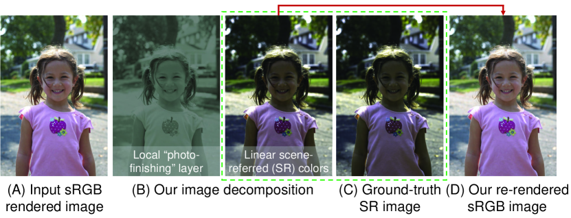
Figure 1: We propose a cycle framework that can unprocess sRGB images back to the linear CIE XYZ color space and re-render the CIE XYZ images into the nonlinear sRGB color space. (A) The input camera-rendered sRGB image. (B) Our image decomposition (left: residual photo-finishing layer, right: scene-referred CIE XYZ reconstruction). (C) The ground-truth scene-referred CIE XYZ image. (D) Our re-rendering result from the reconstructed CIE XYZ image. To aid visualization, CIE XYZ images are scaled by a factor of two. Input image is taken from the MIT-Adobe FiveK dataset [2].

The raw-RGB image state preserves the linear relationship of incident scene radiance. This linear image formation makes raw-RGB images suitable for a wide range of low-level computer vision tasks, such as image deblurring, image dehazing, image denoising, and various types of image enhancement [3, 4, 5, 6]. However, the drawback of raw-RGB is that the physical color filter arrays that make up the sensor’s Bayer pattern are sensor-specific. This means raw-RGB values captured of the same scene but with different sensors are significantly different [7]. This often requires learning-based methods to be trained per sensor or camera make and model (e.g., [8, 9, 10, 5, 11]).

The more common display-referred image state (in this paper, assumed to be in the sRGB color space) also has drawbacks. While this image state is the most widely used and is suitable for display, cameras apply their own proprietary photo-finishing to enhance the visual quality of the image. This means images captured of the same scene but using different camera models (and sometimes the same camera but with different settings) will produce images that have significantly different sRGB values [12, 1, 4].

As previously discussed, the front-end processor of a typical camera ISP performs a colorimetric conversion to map the raw-RGB image to a standard perceptual colorspace—namely, CIE 1931 XYZ [1]. While there exists no formal image encoding for this image state, it is possible to convert existing raw-RGB images stored in digital negative (DNG) format to this intermediate state by applying a software camera ISP (e.g., [13, 1]). This provides a mechanism to standardize all images into a canonical linear scene-referred image state and is the impetus of our work.

Contribution We propose a method to decompose non-linear sRGB images into two parts: 1) a canonical linear scene-referred image state in the CIE XYZ color space and 2) a residual image layer that resembles additional non-linear and local photo-finishing operations. Through such decomposition strategy, we learn a model that can accurately map back and forth between non-linear sRGB and linear CIE XYZ images. An example is shown in Fig. 1. Unlike raw-RGB, the CIE XYZ color space is device-independent, and as a result, helps with model generalization. Furthermore, CIE XYZ images can be encoded as standard three-channel images that can be easily handled by existing computer vision frameworks. We show that our proposed model maps images back to the CIE XYZ color space more accurately compared to alternative approaches. In addition, we perform extensive experiments on tasks such as image denoising, deblurring, and defocus estimation, to show that employing our proposed CIE XYZ model provides the performance boost anticipated from using linear images. Finally, we also show that using our decomposed image layers (CIE XYZ and a residual layer), our model can be used to perform various image enhancement and photo-finishing tasks.

2 Related Work

In this section, we first discuss the camera imaging pipeline that is necessary in order to understand how and why we access the camera image once converted to the CIE XYZ color space. We then review various methods proposed for linearization of camera-rendered images.

2.1 Camera Imaging Pipeline

Images captured by a camera undergo a sequence of processes in order to transform an initial image obtained by the raw sensor data (raw-RGB image) into a visually perceivable color space (e.g., sRGB) and a suitable format for storage and display (e.g., JPEG) [14, 15, 16, 1]. A simplified depiction of the imaging pipeline is shown in Fig. 2. The pipeline processes can be divided into two main stages. The first stage is colorimetric processing that transforms the image into a linear color space (e.g., CIE XYZ or ProPhoto) that preserves the direct mapping between the recorded scene values and the image. The second stage in the camera pipeline is the camera-rendering or photo-finishing stage that applies nonlinear transformations (e.g., gamma compression), selective color manipulation, and locally varying processing (e.g., local tone mapping) that break the relation between the image and the scene. Using images in the linear stages of the imaging pipeline has been shown to be more effective for image restoration and enhancement tasks [1, 4, 5]. However, due to the complexity and proprietary nature of imaging pipelines on-board cameras, it is hard to obtain colorimetric images from cameras without the effort of saving raw sensor data or inverting the imaging pipeline stages [4, 5].

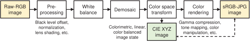
Figure 2: A simplified depiction of a camera imaging pipeline, adapted from [14, 15, 16, 1]. Our method allows mapping back and forth between the common nonlinear sRGB image and to the colorimetric, linear, color-balanced CIE XYZ image state for computer vision tasks.

2.2 Camera-Rendered Image Linearization

To obtain a linear image from its camera-rendered version, we need to reverse the nonlinear camera-rendering stage in the pipeline. Many methods have been proposed to model a parametric relationship that maps from the camera-rendered image (i.e., sRGB image) back to its raw-RGB version (e.g., [4]). However, raw-RGB space is camera-dependent and requires having a separate model per camera. Other approaches involve simple linearization by inverting the global tone mapping and the gamma compression followed by applying a linearization matrix to obtain a linear sRGB or CIE XYZ image [5]. Such approaches are too simple and do not account for the local processing or dynamic range adjustments. Unlike prior approaches, instead of trying only to obtain a linear image, our approach is to decompose the nonlinear image into globally processed and locally processed layers. The locally processed layer represents local color processing, such as local tone mapping. Then, we learn a global mapping from the globally processed image to the linear image. Another line of research targeting the problem of image linearization is radiometric calibration [17, 18]. Unlike our approach, radiometric calibration methods do not target a specific, well-defined color space, and do not address the problem of local processing.

3 Our Framework

This section describes our overall framework, including network architecture, dataset generation, and training details.

3.1 Formulation

Inside a camera imaging pipeline, a raw-RGB image $\mathbf{x}_{\mathrm{raw}}\in\mathbb{R}^{h\times w}$ undergoes a sequence of processing stages to be transformed to the final output sRGB image $\mathbf{x}_{\mathrm{srgb}}\in\mathbb{R}^{h\times w\times 3}$, where $h$ and $w$ represent the image height and width, respectively. As mentioned earlier, the raw-RGB image $\mathbf{x}_{\mathrm{raw}}$ is in a camera-dependent color space that is linear with respect to scene light irradiance falling on the sensor. One of the early steps in the camera processing pipeline is to convert the camera-dependent color space to a device-independent color space—namely, CIE XYZ. Based on this observation, instead of modeling the whole pipeline back to the raw-RGB image, we choose to model an intermediate representation of the image in the CIE XYZ color space $\mathbf{x}_{\mathrm{xyz}}\in\mathbb{R}^{h\times w\times 3}$ that is still linear with respect to scene irradiance, but is in a canonical color space. We are interested in the on-camera rendering procedures that map the CIE XYZ images into the final display-referred (i.e., photo-finished) sRGB color space. This operation can be described as

$$\mathbf{x}_{\mathrm{srgb}}=\mathcal{F}(\mathbf{x}_{\mathrm{xyz}}).$$ (1)

In our method, instead of relying on a single function to model the pipeline stages between sRGB and CIE XYZ, we decompose this mapping into two parts: 1) global processing, denoted collectively as $\mathcal{F}_{\mathrm{glob}}(\cdot)$, that is globally applied to all image pixels and 2) local processing, denoted collectively as $\mathcal{F}_{\mathrm{loc}}(\cdot)$, that represents local photo-finishing operations, such as local tone mapping and selective color adjustments. The forward pipeline from $\mathbf{x}_{\mathrm{xyz}}$ to $\mathbf{x}_{\mathrm{srgb}}$ can be represented as a cascade of the global and the local processes. The global processing stage is represented as

$$\mathbf{M}_{\mathrm{fwd}}=\mathcal{F}_{\mathrm{glob}}(\mathbf{x}_{\mathrm{xyz}}),$$ (2)

$$\mathbf{x}_{\mathrm{glob}}=\psi\left(\mathbf{M}_{\mathrm{fwd}}\ \phi(\mathbf{x}_{\mathrm{xyz}})\right),$$ (3)

where $\mathbf{M}_{\mathrm{fwd}}\in\mathbb{R}^{3\times 6}$ is a global transformation matrix and $\mathbf{x}_{\mathrm{glob}}$ is the globally processed image layer. The operator $\phi(\cdot)$ reshapes the image to be $6\times n$ where $n$ is the number of pixels in the image and each pixel is transformed from three to six dimensions: $[R,G,B]\rightarrow[R,G,B,R^{2},G^{2},B^{2}]$, while the operator $\psi$ reshapes the image from $3\times n$ back to $h\times w\times 3$. We chose $\mathbf{M}_{\mathrm{fwd}}$ to be nonlinear to capture global color processing operations, such as gamma compression.

As most consumer cameras locally process the captured scene-referred images to improve the quality of final rendered images [19], such global color processing may not be able to effectively model the function $\mathcal{F}$. To that end, we use a residual learning mechanism where we model the residual layer $\mathbf{x}_{\mathrm{res}}$ between the locally and globally processed layers of the image as follows:

$$\mathbf{x}_{\mathrm{res}}=\mathcal{F}_{\mathrm{loc}}(\mathbf{x}_{\mathrm{glob}}),$$ (4)

$$\mathbf{x}_{\mathrm{srgb}}=\mathbf{x}_{\mathrm{glob}}+\mathbf{x}_{\mathrm{res}}.$$ (5)

Now, the decomposition process applies the inverse process of Equations 2 – 5 as follows:

$$\mathbf{x}_{\mathrm{res}}=\mathcal{G}_{\mathrm{loc}}(\mathbf{x}_{\mathrm{srgb}}),$$ (6)

$$\mathbf{x}_{\mathrm{glob}}=\mathbf{x}_{\mathrm{srgb}}-\mathbf{x}_{\mathrm{res}},$$ (7)

$$\mathbf{M}_{\mathrm{inv}}=\mathcal{G}_{\mathrm{glob}}(\mathbf{x}_{\mathrm{glob}}),$$ (8)

$$\mathbf{x}_{\mathrm{xyz}}=\psi\left(\mathbf{M}_{\mathrm{inv}}\ \phi(\mathbf{x}_{\mathrm{glob}})\right),$$ (9)

where $\mathcal{G}_{\mathrm{loc}}(\cdot)$ represents the inverse of residual local processing layer and $\mathcal{G}_{\mathrm{glob}}(\cdot)$ is constrained to produce a global transformation matrix $\mathbf{M}_{\mathrm{inv}}\in\mathbb{R}^{3\times 6}$ that represents the inverse global processing stage.

Our ultimate goal is to allow the manipulation of the reconstructed CIE XYZ image by arbitrary image restoration/enhancement algorithms between the inverse and forward pipeline stages (see Fig. 3). It is, however, non-trivial to infer the inverse functions $\mathcal{G}_{\mathrm{loc}}^{-1}(\cdot)$ and $\mathcal{G}_{\mathrm{glob}}^{-1}(\cdot)$ to render back the reconstructed image, as its values may be changed by the image restoration or enhancement algorithms. To that end, we model each of $\mathcal{F}_{\mathrm{glob}}(\cdot)$, $\mathcal{F}_{\mathrm{loc}}(\cdot)$, $\mathcal{G}_{\mathrm{glob}}(\cdot)$, and $\mathcal{G}_{\mathrm{loc}}(\cdot)$ by a neural network.

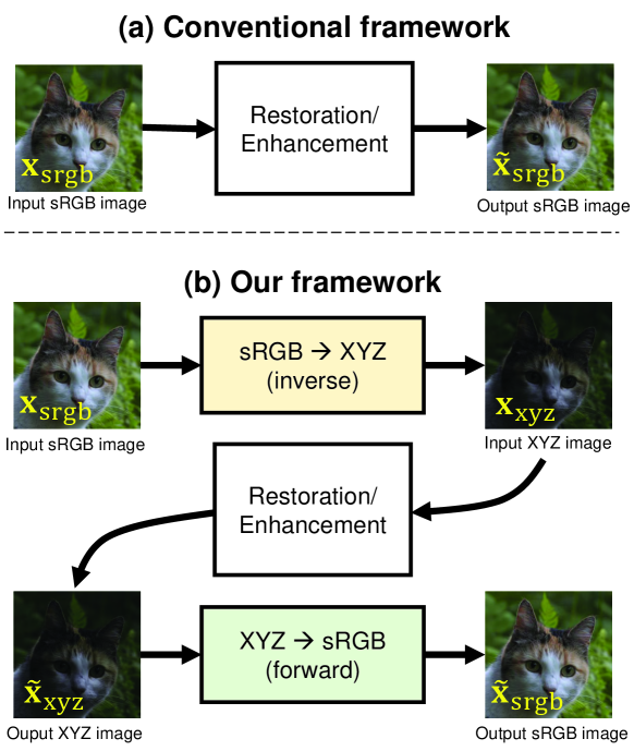
Figure 3: An illustration of using our inverse and forward image processing pipelines in an sRGB image restoration/enhancement framework.

3.2 Network Design

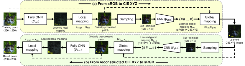
Figure 4: Our CIE XYZ image pipeline. The upper part is the inverse pipeline that unprocesses an sRGB image into a CIE XYZ image. The lower part is the forward pipeline that processes a CIE XYZ image into its equivalent sRGB image. The full framework is trainable end-to-end. The CIE XYZ images are scaled 2x to aid visualization.

Imitating this division of the camera imaging pipeline, we build our network architecture to include two sub-networks for modeling both the global and local processing parts for the forward and inverse directions of the imaging pipeline. As shown in Fig. 4, we start with the inverse pipeline where the first part is a fully convolutional neural network (CNN) that models the local processing applied to an input non-linear image (i.e., sRGB image) by predicting the residual image $\mathbf{x}_{\mathrm{res}}$ (Equation 6). Once the local processing layer is predicted, it can be subtracted from the input image $\mathbf{x}_{\mathrm{srgb}}$ to get the globally processed image $\mathbf{x}_{\mathrm{glob}}$ (Equation 7). Then, $\mathbf{x}_{\mathrm{glob}}$ is fed to another sub-network that predicts a global transformation $\mathbf{M}_{\mathrm{inv}}$ that inverts $\mathbf{x}_{\mathrm{glob}}$ back to the linear CIE XYZ image $\mathbf{x}_{\mathrm{xyz}}$ (Equation 9). With this inverse pipeline, we decompose the input image $\mathbf{x}_{\mathrm{srgb}}$ into two image layers, $\mathbf{x}_{\mathrm{res}}$ and $\mathbf{x}_{\mathrm{glob}}$, which represent local and global processing, respectively, and finally output the linear CIE XYZ image $\mathbf{x}_{\mathrm{xyz}}$.

As discussed in Section 1, there are computer vision tasks, such as image restoration, that are best processed in a linear image state. A use case of the framework is to convert the input image $imxyz$, process the $imxyz$ image, and then render the image back. In this scenario, after decomposing an image and applying an image restoration task to the linear XYZ image, we now need to merge these image layers back to produce the fully processed sRGB image. To model this forward pass of our pipeline, as shown in Fig. 4, we use two sub-networks. The first sub-network predicts a global transformation $\mathbf{M}_{\mathrm{fwd}}$ that maps $\mathbf{x}_{\mathrm{xyz}}$ to $\mathbf{x}_{\mathrm{glob}}$ (Equation 3). The second sub-network predicts the residual local processing $\mathbf{x}_{\mathrm{res}}$ that needs to be applied to $\mathbf{x}_{\mathrm{glob}}$ to obtain the final sRGB image $\mathbf{x}_{\mathrm{srgb}}$ (Equation 5). This framework is illustrated in Fig. 3 and compared to the conventional way of directly processing the sRGB image.

In order to allow the networks $\mathcal{G}_{\mathrm{glob}}(\cdot)$ and $\mathcal{G}_{\mathrm{loc}}(\cdot)$ to separate the globally and locally processed image layer without having ground truth for both $\mathbf{x}_{\mathrm{glob}}$ and $\mathbf{x}_{\mathrm{res}}$, we apply a scaling factor to the output of the local processing networks $\mathcal{G}_{\mathrm{glob}}(\cdot)$, in both inverse and forward passes, such that the values of $\mathbf{x}_{\mathrm{res}}$ are much smaller than $\mathbf{x}_{\mathrm{glob}}$. In our experiments, we set this scaling factor to $0.25$. Fig. 5 shows an example of the output of each sub-network.

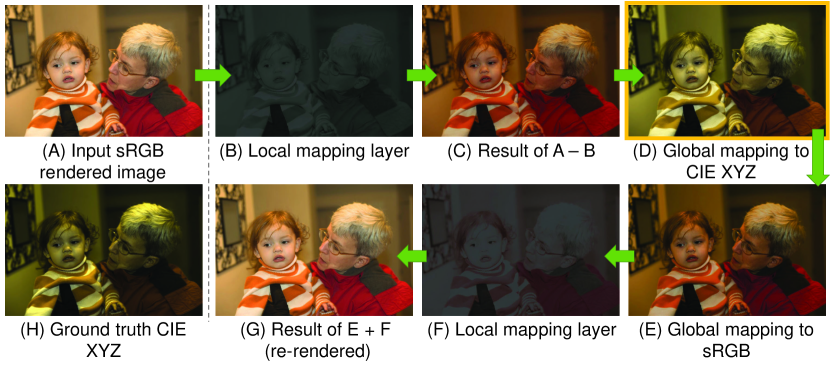
Figure 5: Our inverse pipeline decomposites a given camera-rendered sRGB image into a local processed layer and the corresponding CIE XYZ image, while our forward pipeline maps the reconstructed CIE XYZ image to the sRGB color space in an inverse way of our decomposition. The shown image is taken from our testing set. To aid visualization, CIE XYZ images are scaled by a factor of two.

3.3 Loss Function

The objective of the whole network is to minimize the mean absolute error (MAE): 1) between the predicted XYZ image $\hat{\mathbf{x}}_{\mathrm{xyz}}$ and its ground truth $\mathbf{x}_{\mathrm{xyz}}^{*}$ in the inverse pipeline and 2) between the predicted sRGB image $\hat{\mathbf{x}}_{\mathrm{srgb}}$ and its ground truth $\mathbf{x}_{\mathrm{srgb}}^{*}$ in the forward pipeline, as follows:

$$\lambda\left\lvert\hat{\mathbf{x}}_{\mathrm{xyz}}-\mathbf{x}_{\mathrm{xyz}}^{*}\right\rvert+\left\lvert\hat{\mathbf{x}}_{\mathrm{srgb}}-\mathbf{x}_{\mathrm{srgb}}^{*}\right\rvert,$$ (10)

where $\lambda$ is a weighting factor that we use to deal with the fact that XYZ images generally have lower intensity compared to sRGB images; so this weight can balance the learning behavior between the forward and inverse pipelines. In our experiments, we set $\lambda=1.5$.

3.4 Sub-Networks Architecture

Our local processing sub-networks ($\mathcal{F}_{\mathrm{loc}}$ and $\mathcal{G}_{\mathrm{loc}}$) each consist of 15 blocks of $3\!\times\!3$ convolutional (conv)–LReLU layers. Each conv layer has 32 output channels, with stride of 1 and padding of 1. The last layer of these sub-networks has a single conv layer with three output channels, followed by a $\tanh$ operator. As our global processing sub-networks are not fully convolutional, we use a fixed size of input by introducing a differentiable subsampling module that uniformly subsamples $128\!\times\!128$ color values of the processed image by the previous sub-network. Our global sub-network includes five blocks of $3\!\times\!3$ conv–LReLU–$2\!\times\!2$ max pooling layers. The conv layers have stride and padding of 1, while the max pooling layers have a stride factor of 2 with no padding. Then, we added a fully connected layer with 1024 output neurons, followed by a dropout layer with a factor of 0.5. The last layer of our global sub-network has a fully connected layer with 18 output neurons to formulate our $3\!\times\!6$ polynomial mapping function. Our entire framework is a light-weight model with a total of 2,697,578 learnable parameters ($\sim$11MB of memory) for both sRGB-to-XYZ and XYZ-to-sRGB models, and it is fully differentiable for end-to-end training.

3.5 Dataset

To train our proposed model, we need a dataset of sRGB images with their corresponding linear images in the CIE XYZ color space. To do so, we start from raw-RGB images taken from the MIT-Adobe FiveK [2]. We then process the raw-RGB images twice to obtain both the sRGB and XYZ versions of each image. For processing raw-RGB images into the XYZ color space, we used the camera pipeline from [13]. This pipeline provides an access to the CIE XYZ values after processing the sensor raw-RGB using the color space transformation (CST) matrices provided with the raw-RGB image. To obtain the camera-like sRGB images, we used the Adobe Camera RAW software development kit (SDK), which accurately emulates the nonlinearity applied by consumer cameras [20]. Our dataset includes $\sim$1,200 pairs of sRGB and camera CIE XYZ images. Our dataset will be publicly available upon acceptance.

3.6 Training

We divided our dataset into a training set of 971 pairs, a validation set of 50 pairs, and a testing set of 244 pairs. We trained our framework in an end-to-end manner on patches of size $256\!\times\!256$ pixels randomly extracted from our training set, with a mini-batch of size 4. We applied random geometric augmentation (i.e., scaling and reflection) to the extracted patches.

Our framework was trained in an end-to-end manner for 300 epochs using Adam optimizer [21] with gradient decay factor $\beta_{1}=0.9$ and squared gradient decay factor $\beta_{2}=0.999$. We used a learning rate of $10^{-4}$ with a drop factor of 0.5 every 75 epochs. We added an $L_{2}$ regularization with a weight of $\lambda_{\mathrm{reg}}=10^{-3}$ to our loss in Equation 10 to avoid overfitting.

4 Experimental Results

In this section, we first validate the effectiveness of our proposed model in mapping from camera-rendered sRGB images to CIE XYZ, and processing CIE XYZ images back to sRGB. Next, we demonstrate our method’s utility on a number of classical image restoration tasks, such as image denoising, motion deblurring, and image dehazing, that assume a linear relationship between the scene radiance and the recorded pixel intensity. Finally, we show that our linear space is also advantageous for a variety of image enhancement tasks.

4.1 From Camera-Rendered sRGB to CIE XYZ, and Back

We first verify our network’s ability to unprocess sRGB images to CIE XYZ. We also demonstrate our ability to reconstruct from CIE XYZ back to sRGB. We test our mapping to sRGB using our reconstructed CIE XYZ results as a starting point, and also using the ground-truth CIE XYZ images. For comparison, we use the standard CIE XYZ mapping [22, 23], which applies a simple 2.2 gamma tone curve, and the recent unprocessing technique (UPI) from [5]. The UPI technique provides a proxy for the major procedures of the camera pipeline. For a fair comparison, we compare our results with results of UPI obtained at the CIE XYZ stage.

Table I shows peak signal-to-noise ratio (PSNR) results averaged over 244 unseen testing images from the MIT-Adobe FiveK dataset [2]. The terms Q1, Q2, and Q3 refer to the first, second (median), and third quantile, respectively, of the PSNR values obtained by each method. For the standard XYZ, the results of mapping from the reconstructed CIE XYZ images back to sRGB are not reported because standard XYZ uses an invertible transform. The sRGB reconstruction error from the UPI model [5] is high due to the fact that the tone mapping is not perfectly invertible. It can be observed from the results that we outperform both competing methods by a sound margin. Qualitative comparisons are provided in Fig. 6.

As shown in Table I, the mapping to sRGB from reconstructed CIE XYZ is better than mapping from ground-truth CIE XYZ. For our method, this behavior is expected because the forward model is trained on the reconstructed CIE XYZ, not the ground truth. Also, for the UPI method, as it is based on matrix inversion, the mapping from the reconstructed CIE XYZ makes the transformation more accurate than mapping from the ground truth.

TABLE I: Results (in terms of PSNR) of camera-rendered sRGB $\leftrightarrow$ CIE XYZ mapping. We compare our results against the standard XYZ mapping (the 2.2 gamma tone curve) [22, 23] and the recent unprocessing technique (UPI) [5]. Average PSNR (dB) results are reported on 244 unseen testing pairs (camera-rendered sRGB and corresponding CIE XYZ images) from the MIT-Adobe FiveK dataset [2]. We show results of mapping from both reconstructed (Rec.) CIE XYZ images and ground truth (GT) CIE XYZ images to the corresponding camera-rendered sRGB images. Highest PSNR values are shown in bold.

	sRGB $\rightarrow$ XYZ				Rec. XYZ $\rightarrow$ sRGB				GT XYZ $\rightarrow$ sRGB
Method	Avg.	Q1	Q2	Q3	Avg.	Q1	Q2	Q3	Avg.	Q1	Q2	Q3
Standard [22, 23]	21.84	16.88	20.91	25.24	-	-	-	-	22.22	19.19	21.79	24.37
Unprocessing [5]	22.19	19.31	22.12	24.75	37.72	37.78	40.56	41.88	18.04	15.67	17.79	20.02
Ours	29.66	23.77	29.57	34.71	43.82	41.43	43.94	46.58	27.44	23.57	28.32	30.88

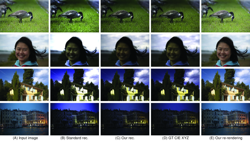
Figure 6: Qualitative comparisons for CIE XYZ reconstruction and rendering. (A) The input sRGB rendered image. (B) Standard display-referred CIE XYZ reconstruction [22, 23]. (C) Our reconstruction. (D) The ground-truth scene-referred CIE XYZ image. (E) Our re-rendering result from the reconstructed CIE XYZ image. To aid visualization, CIE XYZ images are scaled by a factor of two. Input images are taken from the MIT-Adobe FiveK dataset [2].

We compare our proposed network against a U-Net-based baseline. This baseline consists of two U-Net-like [24] models trained in an end-to-end manner using the same training settings used to train our network (i.e., epochs, training patches, and loss function). Each U-Net model consists of a 3-level encoder/decoder with skip connections. The output channels of the first conv layer in the encoder unit has 28 channels. The two U-Net models have a total of 2,949,246 learnable parameters, compared to 2,697,578 learnable parameters in our network, and they were trained to map from sRGB to XYZ and from XYZ back to sRGB, similar to our model.

Table II shows the results obtained by the U-Net baseline and our network on our testing set.

	sRGB $\rightarrow$ XYZ				Rec. XYZ $\rightarrow$ sRGB
Method	Avg.	Q1	Q2	Q3	Avg.	Q1	Q2	Q3
U-Net	20.05	16.84	19.76	22.78	43.39	40.56	43.40	45.91
Ours	29.66	23.77	29.57	34.71	43.82	41.43	43.94	46.58

TABLE II: Comparison between our network and two U-Net models trained in an end-to-end manner to map from sRGB to CIE XYZ and back. Both networks, ours and the two U-Net models, have approximately the same number of learnable parameters and both were trained using the same training settings. The best PSNR (dB) values are shown in bold.

4.2 Image Restoration Applications

As previously discussed, many image restoration tasks assume a linear image formation model and work best with linearized data. In the following sections, we apply our method to the problems of image denoising, motion deblurring, defocus blur detection, raw-RGB image reconstruction, and image dehazing. We show improvement in performance from working on CIE XYZ images compared to working directly with sRGB images or applying existing linearization methods. We would like to highlight that our objective is not to outperform the state-of-the-art. Instead, our goal is to show that having selected a particular algorithm for a given task, its performance improves when applied to our linearized images as compared to using sRGB images, or employing existing linearization approaches.

4.2.1 Image Denoising

We first apply our decomposition method to the task of image denoising. Image denoising algorithms can perform better on linear images because of the simplicity of the linear signal-dependent noise model [25, 13]. We demonstrate this behavior using our CIE XYZ images for two denoising methods: BM3D [26] and DnCNN [27]. The first is statistics-based while the latter is learning-based. Both methods are well established in the image denoising literature. We evaluated the chosen methods on the SIDD-Validation dataset [13].

We compare denoising CIE XYZ images from our method against the standard XYZ linearization [22, 23]. First, the sRGB images are linearized, denoising is performed, and the denoised images are mapped back to sRGB. As a baseline, we also apply denoising directly in the sRGB space. For the BM3D denoiser, we used its color-variant version—namely, CBM3D [26]. For DnCNN, we used the pre-trained model from [27], denoted as DnCNN-P. We also re-trained DnCNN models on images processed with both linearization methods, denoted as DnCNN-R.

The evaluation is based on the PSNR (dB) and structural similarity index (SSIM) [28], both in the sRGB color space. The results are shown in Table III. Both CBM3D and DnCNN-P show significant denoising improvement when applied to images unprocessed by our method into the CIE XYZ space compared to linearized images obtained by the standard XYZ linearization. DnCNN-R using our CIE XYZ images gains more improvement in terms of SSIM, but is still comparable to using standard XYZ images in terms of PSNR. Also, we can see that denoising in our reconstructed CIE XYZ space is better compared to denoising directly in the sRGB color space.

	CBM3D		DnCNN-P		DnCNN-R
Method	PSNR	SSIM	PSNR	SSIM	PSNR	SSIM
XYZ - Standard	33.84	0.8733	26.23	0.5936	33.92	0.7833
XYZ - Ours	35.49	0.9245	27.71	0.6623	33.00	0.8865
sRGB	34.44	0.9021	25.31	0.5578	30.72	0.7943

TABLE III: Results of image denoising performed on the SIDD-Validation set [13] after unprocessing the images using our method compared to standard linearization [22, 23]. The last row is the result of denoising directly in the sRGB space. All PSNR and SSIM values are calculated in the sRGB space. CBM3D and DnCNN-P show significant improvement in denoising using images unprocessed by our method.

4.2.2 Motion Deblurring

Traditionally, a motion blurred image $G$ is represented using a linear image formation model as the convolution between an underlying sharp image $F$, and a motion blur kernel $H$ [29]—namely, $G=F\otimes H$, where $\otimes$ denotes the convolution operation. The blur kernel $H$ is the same across the image.

However, this linear relationship between $G$ and $F$ does not hold for blurred photo-finished sRGB images. Tai et al. [30] showed that the blur kernel $H$ varies spatially across the image due to the non-linear stages of the camera pipeline, making motion deblurring significantly more challenging. Therefore, it is advantageous to deblur the image in a linear scene-referred space.

We select the statistics-based non-blind motion deblurring method of Krishnan and Fergus [31], and evaluate its performance in our linearized color space, as well as other spaces, such as nonlinear sRGB and standard XYZ [22, 23]. For this experiment, we chose the same 244 unseen testing images from the MIT-Adobe FiveK dataset [2] used earlier in Section 4.1. To generate motion blurred sRGB images, we blur each ground-truth raw-RGB image with a random kernel selected from one of the four kernels in the widely used motion blur benchmark dataset of Lai et al. [32]. The blurred raw-RGB images are then rendered to sRGB using the camera pipeline simulator of [13]. Fig. 7 shows four representative deblurring results, one for each motion kernel from the dataset of [32]. It can be clearly observed from the zoomed-in regions that deblurring in the sRGB and the standard CIE XYZ color spaces produces a lot of ringing artifacts, particularly for larger blur kernels (e.g., the examples in the last two rows). In comparison, our results are sharper and less prone to ringing. Deblurring in our linear space produced an average PSNR of 30.26 dB, whereas sRGB and standard XYZ yielded only 29.41 dB and 28.68 dB, respectively—a clear demonstration of the utility of our proposed framework for motion deblurring.

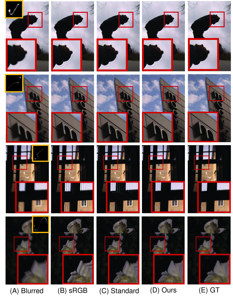
Figure 7: Qualitative results for motion deblurring application. (A) The blurred input image and the corresponding motion blur kernel. (B-D) Deblurring results in sRGB, standard XYZ, and our proposed CIE XYZ color space, respectively. The shown deblurring results are obtained by the non-blind image deblurring algorithm of Krishnan and Fergus [31]. (E) The ground-truth sharp image. Images are taken from the MIT-Adobe FiveK dataset [2], and the motion blur kernels are the four kernels used in the benchmark motion blur dataset of Lai et al. [32].

4.2.3 Defocus Blur Detection

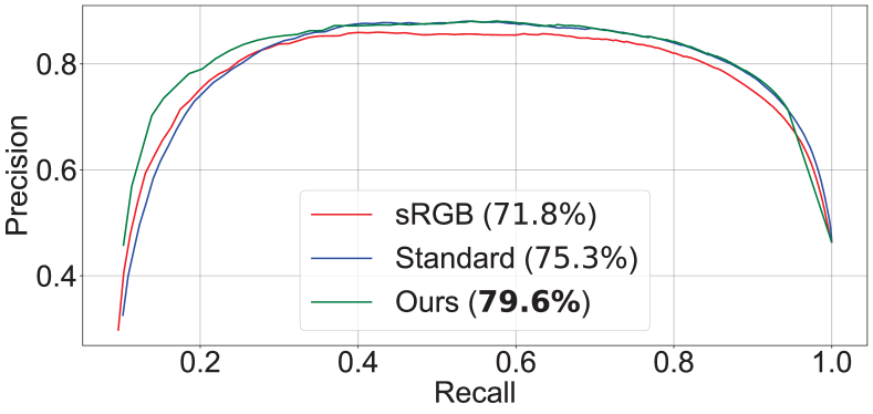
Figure 8: The precision-recall (PR) comparison of training light UNet on data from three different color spaces: sRGB, standard linearized CIE XYZ [22, 23], and our linearized CIE XYZ. The average accuracy for each model is shown in the plot’s legend. Our linear space achieves the best PR curve and the highest accuracy.

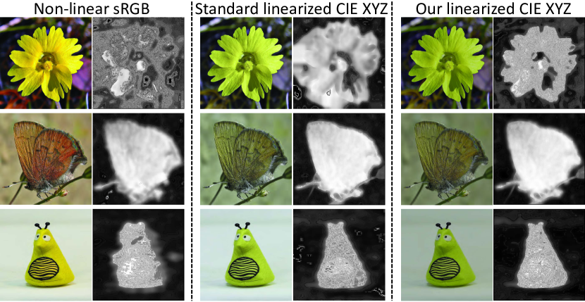
Figure 9: Qualitative results of three light UNets trained on three different color spaces for the task of defocus map estimation. Training the light UNet using our linearized CIE XYZ images gives better visual results as shown in the third column. The CIE XYZ input images are gamma corrected for better visualization.

Defocus detection is the problem of detecting the image pixels that are out of focus. This problem is important to many computer vision tasks, such as non-blind defocus deblurring, image refocusing, depth estimation, and 3D reconstruction. The methods targeting this problem are well established [33, 34, 35, 36, 37, 38]. In particular, defocus detection methods output a binary mask of a given input image such that the out-of-focus pixels are zeros and the rest are ones.

We examine the advantage of detecting out-of-focus pixels in our linearized CIE XYZ color space compared to other spaces—namely, non-linear sRGB and standard linearized CIE XYZ. To this aim, we introduce a light UNet-inspired architecture. We train three models using image patches from three different color spaces following the same training procedure. We use the well-known blur detection dataset [34] to train and test the models. In the plot of Fig. 8, we present the precision-recall comparison along with the pixel binary classification accuracy. In addition to the quantitative results, qualitative results are presented in Fig. 9. The results in Fig. 8 and Fig. 9 demonstrate that our linearization is a better color space to perform defocus blur detection compared to other color spaces.

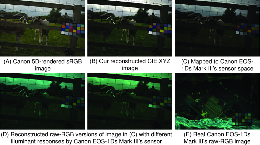
Figure 10: Sensor raw-RGB image reconstruction. (A) An sRGB image rendered by Canon 5D from Gehler-Shi [39]. (B) Our reconstructed CIE XYZ image. (C) Our reconstructed raw image in the raw-RGB space of the Canon EOS-1Ds Mark III. (D) Two generated raw-RGB images with different illuminant responses in the Canon EOS-1Ds Mark III’s sensor space. (E) A real raw-RGB image captured by the Canon EOS-1Ds Mark III taken from the eight-camera NUS dataset [40]. To aid visualization, the shown images are scaled by a factor of two.

4.2.4 Raw-RGB Image Reconstruction

One of the advantages of accurately reconstructing scene-referred images is the ability to map the reconstructed images further into a sensor raw-RGB space. Specifically, we can synthetically generate raw-RGB images in any target sensor space by capturing an image with a color rendition calibration chart placed in the scene. The captured image is saved in both the camera’s sensor raw-RGB space and the camera-rendered sRGB color space. As the CIE XYZ space is defined for correctly white-balanced colors, we first correct the white balance of the raw-RGB image using the color rendition chart. We then reconstruct the XYZ image using our XYZ network and compute a $3\!\times\!3$ matrix to map our reconstructed image into the sensor space. We refer to this matrix as the XYZ$\rightarrow$raw matrix. This calibration matrix is then used to map any arbitrary image into this sensor space by first reconstructing the corresponding XYZ image, followed by mapping it into the sensor space. The assumption here is that as our method achieves superior linearization to the available solutions (see Table I), this calibration process would result in a better sRGB$\rightarrow$raw-RGB mapping.

To validate this assumption, we compare between the raw-RGB reconstruction based on our reconstruction against the raw-RGB reconstruction that is computed based on the standard XYZ mapping method [22, 23]. We examine the data augmentation task for the illuminant estimation problem. Scene illuminant estimation is a well-studied problem in computer vision literature. Briefly, we can describe the illuminant estimation problem as follows. Given a linear raw-RGB image $\mathbf{I}_{\text{raw}}$ captured by a specific camera sensor, the goal is to determine a 3D vector $\boldsymbol{\ell}$ that represents the illuminant color in the captured scene. Recent work achieves promising results using deep learning to estimate the illuminant vector $\boldsymbol{\ell}$ by training deep models that can be later used in the inference phase to estimate illumination colors of given testing images captured by the same sensor used in the training stage [39].

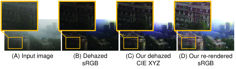
Figure 11: Dehazing is one of the potential applications that can benefit from our image unprocessing method. (A) The input image taken from Flickr (by Mike Rivera, CC BY-NC-SA 2.0). (B) Dehazing applied in the sRGB space. (C) Dehazing applied to our CIE XYZ image. (D) Our final result in the sRGB space. In this example, we used the dehazing method from [41].

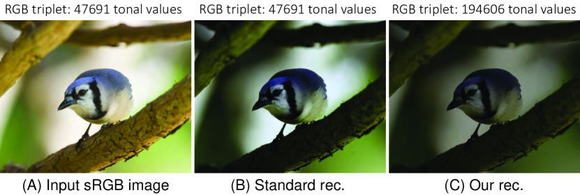
Figure 12: Our XYZ reconstruction provides a wider range of tonal values compared to the standard CIE XYZ mapping [22, 23]. (A) The input sRGB image. (B) Standard XYZ reconstruction [22, 23]. (C) Our XYZ reconstruction. The input image is taken from [42].

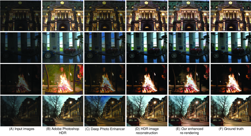
Figure 13: (A) The input sRGB rendered image. (B) Adobe Photoshop HDR results. (C) Deep Photo Enhancer results [43]. (D) HDR result of  [44]. (E) Our re-rendered images after photo-finishing enhancement. (F) Ground-truth images. Input images are taken from [44].

There is currently a challenge in the available datasets for the illuminant estimation task, which is the limited number of available training images captured by the same sensor—for example, the eight-camera NUS dataset [40], one of the common datasets used for illuminant estimation, has 200 images on average for each camera sensor. In this experiment, we examine our raw-like reconstructed images to serve as a data augmenter to train deep learning models for illuminant estimation. Specifically, we train a simple deep learning model to estimate the scene illuminant of a given raw-RGB image captured by Canon EOS-1Ds Mark III [40]. There are only 256 original raw-RGB images captured by Canon EOS-1Ds Mark III in the NUS dataset [40]. For each image, there is a ground-truth scene illuminant vector extracted from the color rendition chart. During training and testing processes, the color chart is masked out in each image to avoid any bias. To augment the data, we first computed the $3\!\times\!3$ XYZ$\rightarrow$raw calibration matrix as described earlier for our XYZ reconstruction and the standard XYZ mapping. This reconstruction process was performed using a single image captured by the Canon EOS-1Ds Mark III camera with a color rendition chart. Afterwards, we used 3,752 white-balanced camera-rendered sRGB images captured by ten different camera models other than our Canon EOS-1Ds Mark III. These images were taken from the Rendered WB dataset [20]. Each sRGB image is converted to the CIE XYZ space using our method and the standard XYZ mapping, followed by mapping each reconstructed image to the Canon EOS-1Ds Mark III sensor space using the calibration matrix computed for each XYZ reconstruction method, respectively.

As the calibration matrices map from the reconstructed XYZ space to the white-balanced sensor raw-RGB space, we can apply illuminant color casts, randomly selected from the ground-truth illuminant vectors provided in the Canon EOS-1Ds Mark III’s set, to synthetically generate additional training data to train the deep model. Fig. 10 shows an example. This process is inspired by previous work in [45, 46], which randomly selected illuminant vectors from the ground-truth set and applied chromatic adaptation to augment the training set. These methods, however, use the same images (256 images in the case of the Canon EOS-1Ds Mark III’s set) without introducing new image content to the trained model.

We randomly selected 50 testing images from the original 256 images provided in the NUS dataset for the Canon EOS-1Ds Mark III camera. We fixed this testing set over all experiments and excluded these images from any training processes. Table IV shows the angular error of the trained model using the following training sets: (i) real training data, (ii) reconstructed raw-like images using the standard XYZ mapping, (iii) real training data and reconstructed raw-like images using the standard XYZ mapping, (iv) reconstructed raw-like images using our XYZ reconstruction, and (v) real training data and reconstructed raw-like images using our XYZ reconstruction. As can be seen, the best results were obtained by using our raw-like reconstruction and real training data. Notice that training only on our raw-like reconstruction gives better results compared with the results obtained by training on real data or reconstructed raw-like images using the standard XYZ mapping.

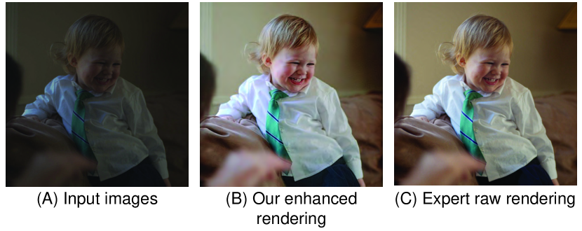
Figure 14: Example from the under-exposure testing set [47]. (A) The input image. (B) Our enhanced rendered image. (C) The expert-retouched image.

4.2.5 Dehazing

A hazy image is expressed using a linear model as $\mathbf{I}(\mathbf{x})=\mathbf{J}(\mathbf{x})t(\mathbf{x})+\mathbf{A}(1-t(\mathbf{x}))$ [41], where $\mathbf{I}$ is the observed intensity, $\mathbf{J}$ is the scene radiance, $\mathbf{A}$ is the global atmospheric light, and $t$ is the medium transmission describing the portion of the light that is not scattered and reaches the camera. Just as with motion deblurring, this linear relationship is broken by the camera’s photo-finishing stages. Therefore, it is desirable to perform dehazing on linearized images. In Fig. 11, we show the result of dehazing an sRGB image versus dehazing our linear CIE XYZ image and then re-rendering to sRGB. The improvement in visual quality can be clearly observed from the zoomed-in regions.

4.3 Photo-Finishing Applications

Many photographers prefer to edit photographs in the linear raw-RGB sensor space rather than the nonlinear 8-bit sRGB space, due to the fact that raw-RGB images provide higher tonal values compared to sRGB camera-rendered images [48]. Similar to the raw-RGB space, the CIE XYZ space is linear scene-referred with higher tonal values compared to the final sRGB space. Thus, we can also benefit from our linear CIE XYZ space for image enhancement tasks.

4.3.1 Low-Light Image Enhancement

In this set of experiments, we present a set of simple operations that can achieve results on par with recent methods designed for low-light image enhancement. Specifically, we apply the following set of heuristic operations to perform low-light image enhancement. As our reconstructed XYZ image has a wider range of tonal values (see Fig. 12), we apply a set of synthetic digital gains to simulate multi-exposure settings. This simulation does not introduce any new information that did not exist in the original image; however, it allows us to better explore the range of tonal values provided in our reconstructed image—we can think of this operation as an ISO gain that is applied on board cameras to amplify the captured image signal. To that end, we multiply the reconstructed image by four different factors. These factors can be tuned in an interactive manner based on each image, but we preferred to fix these hyperparameters over all experiments. In particular, we multiplied our reconstructed XYZ image by (0.1, 1.4, 2.7, 4.0) to generate four different versions of our reconstructed XYZ image. Following this, we apply an off-the-shelf exposure-fusion algorithm [49] to create the modified XYZ layer. To enhance the local details, we apply a local details enhancement method [50] on our forward local sRGB reconstructed layer. Fig. 13 shows examples of our results. As can be seen, we achieve on par results with state-of-the-art methods designed specifically for the given image enhancement task.

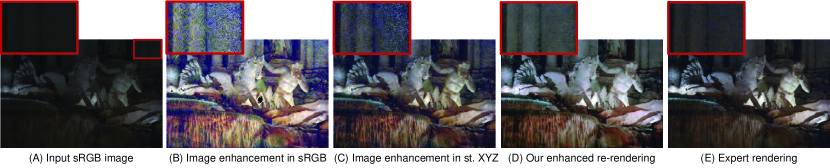
Figure 15: (A) The input image. (B) Image enhancement in sRGB. (C) Image enhancement in standard XYZ reconstruction. (D) Our enhanced re-rendering. (E) Expert enhancement. The enhancement is based on fusion of “multi-exposed” images [49] and local details enhancement [50]. The image is from the under-exposure testing set [47].

TABLE IV: Angular error of illuminant estimating using the image set captured by the Canon EOS-1Ds Mark III in the NUS dataset [40]. We compare the results obtained by training a deep neural network on real raw-RGB training images, reconstructed (rec.) raw-RGB training images based on the standard XYZ reconstruction, and our CIE XYZ reconstruction. The best results are shown in bold.

Training data	Mean	Median	Best 25%	Worst 25%
Real	4.15	3.89	1.13	7.85
Rec. (standard)	3.37	3.03	1.05	6.68
Real and rec. (standard)	2.72	2.60	0.72	4.99
Rec. (ours)	3.00	2.61	0.83	5.37
Real and rec. (ours)	2.41	2.03	0.65	4.66

We further evaluated this simple pipeline on 500 under-exposed images taken from [47]. Fig. 14 shows a qualitative example. We show a quantitative comparison in Table V. Applying digital gain to our reconstructed space provides better results compared to using the standard XYZ reconstruction or the nonlinear sRGB space. This is due to the fact that our reconstructed images have a better linearization with a high tonal range; see Fig. 15. We provide additional results in Figs. 16 and 17.

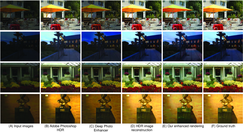
Figure 16: Low-light image enhancement application. (A) Input sRGB rendered image. (B) Adobe Photoshop HDR results. (C) Deep Photo Enhancer results [43]. (D) HDR result of  [44]. (E) Our re-rendered images after photo-finishing enhancement. (F) Ground truth images. Input images are taken from [44].

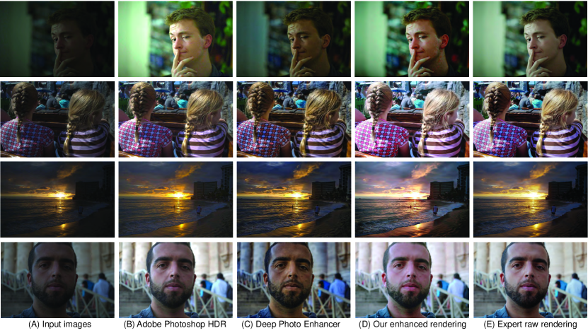
Figure 17: Qualitative comparison for low-light image enhancement task. Images are taken from the under-exposure testing set [47]. (A) Input image. (B) Adobe Photoshop HDR results. (C) Results of deep photo enhancer [43]. (D) Our enhanced rendered image. (E) Expert-retouched image.

Method	PSNR
White-Box [51]	18.57
Distort-and-Recover [52]	20.97
HDRNet [53]	21.96
Deep photo enhancer [43]	22.150
DeepUPE [47]	23.04
Enhanced in sRGB	16.92
Enhanced in rec. standard XYZ	18.41
Our enhanced re-rendering	21.03

TABLE V: Quantitative results of the photo-finishing enhancement application using 500 under-exposure images provided in [47].

5 Concluding remarks

We have proposed a method and DNN model that can map back and forth between non-linear sRGB and linear CIE XYZ images more accurately compared to alternative approaches. Our method is based on learning a decomposition of sRGB images into a globally processed and locally processed image layers. The learned globally processed image layer is then used to learn a mapping to the device independent CIE XYZ color space. We have provided extensive experiments targeting image restoration tasks including image denoising, deblurring, and defocus detection to show that our proposed model provides the performance boost anticipated from using linear images. In addition, utilizing the decomposed image layers, we show that our model can be used to perform various image enhancement and photo-finish tasks. Code and dataset are publicly available at https://github.com/mahmoudnafifi/CIE_XYZ_NET.

Additional Details

Defocus Blur Detection

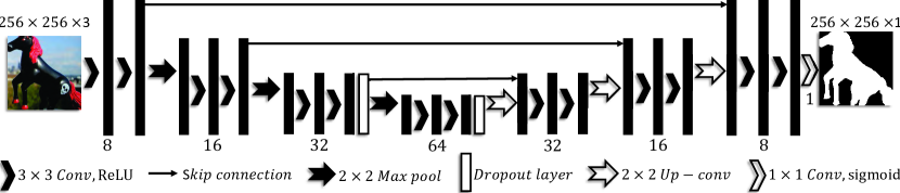
Figure 18: We used a light-weight U-Net-like architecture for the task of defocus blur detection. The size of the input and output layers is shown above the image patches. The number of output filters is shown under the convolution operations.

In Sec. 4.2.3, we used a light-weight U-Net-like architecture for the defocus blur detection task. Fig. 18 shows the details of the used architecture. We trained the model with image patches of size $256\times 256$. We adopted He’s weight initialization [54] and used the Adam optimizer [21] to train our model.

The initial learning rate is set to $10^{-4}$, which is decreased by half every 30 epochs. We train the model with mini-batches of size 12 using the mean squared error (MSE) loss between the output and the ground truth. During the training phase, we set the dropout rate to $0.5$. We found that the model converges after 60 epochs. In Fig. 19, the training and validation curves of different color spaces are shown. Compared to other spaces, our reconstructed CIE XYZ space has a smooth validation convergence and is able to achieve faster convergence with the smallest MSE.

Raw-RGB Image Reconstruction

We discussed the raw-RGB reconstruction as it is one of the potential applications of the proposed XYZ reconstruction in Sec. 4.2.4. In our experiments, we chose the scene illuminant estimation task to validate our raw-RGB reconstruction against the raw reconstruction based on the standard XYZ mapping [22, 23]. We trained a deep model to estimate the scene illuminant from the given raw-RGB image. In this section, we provide the details of the model’s architecture used in these experiments and the training details.

The model is designed to accept a $150\!\times\!150$ raw-RGB image (similar to prior work that proposed to use thumbnail images for the illuminant estimation task [55, 11]). The model includes a sequence of conv, leaky ReLU (LReLU), batch normalization (BN), and fully connected (FC) layers. In particular, the model consists of two conv–LReLU–conv–BN–LReLU blocks, followed by a conv–LReLU–FC–LReLU–dropout–FC–LReLU–FC block. All conv layers have $3\!\times\!3$ filters with a different number of output channels and stride steps. The first, second, and third conv layers have 64 output channels, while the fourth and fifth conv layers have 128 and 256 output channels, respectively. The stride steps were set to 2 for the first three conv layers. For the last two conv layers, we used a stride step of 3. The first two FC layers have 256 output neurons, while the last FC layer has 3 output neurons. We trained each model for 50 epochs to minimize the angular error between the estimated illuminant vector and the ground truth illuminant. The training process was performed with a learning rate of $10^{-4}$ and mini-batch of 32 using the Adam optimizer [21] with a decay rate of gradient moving average 0.9 and a decay rate of squared gradient moving average 0.999.

Image Enhancement

One of the potential applications of our method is low-light image enhancement. We exploited the higher tonal range in the reconstructed CIE XYZ image and proposed a simple set of heuristic operations to perform low-light image enhancement. In our experiments, we used the bilateral guided upsampling method [56] to speed up the running time required to apply the local details enhancement method [50] on the forward local sRGB reconstructed layer. Specifically, we apply the local details enhancement to a downsized version ($150\!\times\!150$) of the local layer, then we apply the bilateral guided upsampling to reconstruct the processed local layer in the original image’s size.

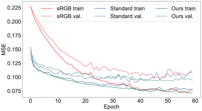
Figure 19: Training and validation curves of different color spaces. The validation curve of our color space shows a better performance over time and achieves the smallest MSE compared to other curves.

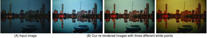
Figure 20: (A) Input sRGB rendered image. (B) Our re-rendered images after enhancement. In this example, we applied chromatic adaptation to three different reference white points. Input image is taken from the under-exposure set [47] of the MIT-Adobe FiveK dataset [2].

Additional Applications

When we work in our reconstructed space (i.e., XYZ), we have a sound interpretation of post-capture white-balance editing using standard white points (e.g., D65, D50) and standard chromatic adaptation transforms (e.g., Bradford CAT [57], Sharp CAT [58]), which are originally designed to work in the camera CIE XYZ space. Fig. 20 shows examples of our enhanced rendering with applying chromatic adaptation [58] in our reconstructed XYZ space.

Additional potential applications are shown in Fig. 21. In the first row of Fig. 21, we show super-resolution results obtained directly by working in the sRGB space and in our reconstructed CIE XYZ space followed by applying our re-rendering process. The last row of Fig. 21 shows an arguably better color transfer result by applying the color transfer process in our reconstructed space.

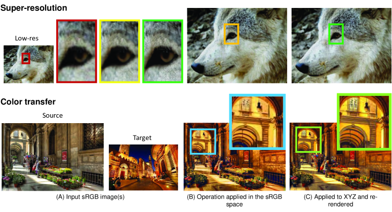
Figure 21: Another potential application of our method. (A) The input sRGB image. (B) Super-resolution and color transfer applied in the sRGB space. (C) Super-resolution and color transfer applied in our reconstructed CIE XYZ space followed by re-rendering. In this example, we used the deep learning super-resolution model proposed in [59] and the color transfer method in [60]. The input image in the first row is taken from the DIV2K dataset [61, 62], while the second input image is taken from Flickr–CC BY-NC 2.0 (by Chris Ford and Giuseppe Moscato, respectively).

Lastly, our rendering network can be used as an alternative way to produce aesthetic photographs from raw-RGB DNG files, as shown in Fig. 22. In this example, we first used the DNG metadata to map the raw-RGB values into the CIE XYZ space. Then, we used our rendering network and a local Laplacian filter to generate the shown output images.

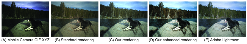
Figure 22: Our rendering network generalizes well for unseen CIE XYZ input images and produces pleasing results that are close to Adobe Lightroom’s quality. (A) Input smartphone camera CIE XYZ image. (B) Standard rendering [22, 23]. (C) Our rendering. (D) Our rendering after enhancing the local layer using the local Laplacian filter [50]. (E) Adobe Lightroom rendering. To aid visualization, CIE XYZ images are scaled by a factor of two. Input image is taken from the HDR+ burst photography dataset [19].

References

- [1] H. C. Karaimer and M. S. Brown, “A software platform for manipulating the camera imaging pipeline,” in ECCV, 2016.
- [2] V. Bychkovsky, S. Paris, E. Chan, and F. Durand, “Learning photographic global tonal adjustment with a database of input / output image pairs,” in CVPR, 2011.
- [3] Y.-W. Tai, X. Chen, S. Kim, S. J. Kim, F. Li, J. Yang, J. Yu, Y. Matsushita, and M. S. Brown, “Nonlinear camera response functions and image deblurring: Theoretical analysis and practice,” IEEE Transactions on Pattern Analysis and Machine Intelligence, vol. 35, no. 10, pp. 2498–2512, 2013.
- [4] R. M. Nguyen and M. S. Brown, “Raw image reconstruction using a self-contained sRGB-JPEG image with only 64 KB overhead,” in CVPR, 2016.
- [5] T. Brooks, B. Mildenhall, T. Xue, J. Chen, D. Sharlet, and J. T. Barron, “Unprocessing images for learned raw denoising,” in CVPR, 2019.
- [6] S. W. Zamir, A. Arora, S. Khan, M. Hayat, F. S. Khan, M.-H. Yang, and L. Shao, “CycleISP: Real image restoration via improved data synthesis,” arXiv preprint arXiv:2003.07761, 2020.
- [7] R. M. H. Nguyen, D. K. Prasad, and M. S. Brown, “Raw-to-raw: Mapping between image sensor color responses,” in CVPR, 2014.
- [8] S. Diamond, V. Sitzmann, S. Boyd, G. Wetzstein, and F. Heide, “Dirty pixels: Optimizing image classification architectures for raw sensor data,” arXiv preprint arXiv:1701.06487, 2017.
- [9] S. Nam and S. Joo Kim, “Modelling the scene dependent imaging in cameras with a deep neural network,” in ICCV, 2017.
- [10] Y. Hu, B. Wang, and S. Lin, “FC4: Fully convolutional color constancy with confidence-weighted pooling,” in CVPR, 2017.
- [11] M. Afifi and M. S. Brown, “Sensor-independent illumination estimation for dnn models,” arXiv preprint arXiv:1912.06888, 2019.
- [12] S. J. Kim, H. T. Lin, Z. Lu, S. Süsstrunk, S. Lin, and M. S. Brown, “A new in-camera imaging model for color computer vision and its application,” IEEE Transactions on Pattern Analysis and Machine Intelligence, vol. 34, no. 12, pp. 2289–2302, 2012.
- [13] A. Abdelhamed, S. Lin, and M. S. Brown, “A high-quality denoising dataset for smartphone cameras,” in Proceedings of the IEEE Conference on Computer Vision and Pattern Recognition, 2018, pp. 1692–1700.
- [14] R. D. Gow, D. Renshaw, K. Findlater, L. Grant, S. J. McLeod, J. Hart, and R. L. Nicol, “A comprehensive tool for modeling cmos image-sensor-noise performance,” IEEE Transactions on Electron Devices, vol. 54, no. 6, pp. 1321–1329, 2007.
- [15] C. Liu, R. Szeliski, S. B. Kang, C. L. Zitnick, and W. T. Freeman, “Automatic estimation and removal of noise from a single image,” IEEE Transactions on Pattern Analysis and Machine Intelligence, vol. 30, no. 2, pp. 299–314, 2007.
- [16] S. W. Hasinoff, F. Durand, and W. T. Freeman, “Noise-optimal capture for high dynamic range photography,” in CVPR, 2010, pp. 553–560.
- [17] H. Lin, S. J. Kim, S. Süsstrunk, and M. S. Brown, “Revisiting radiometric calibration for color computer vision,” in ICCV, 2011.
- [18] A. Chakrabarti, Y. Xiong, B. Sun, T. Darrell, D. Scharstein, T. Zickler, and K. Saenko, “Modeling radiometric uncertainty for vision with tone-mapped color images,” IEEE Transactions on Pattern Analysis and Machine Intelligence, vol. 36, no. 11, pp. 2185–2198, 2014.
- [19] S. W. Hasinoff, D. Sharlet, R. Geiss, A. Adams, J. T. Barron, F. Kainz, J. Chen, and M. Levoy, “Burst photography for high dynamic range and low-light imaging on mobile cameras,” ACM Transactions on Graphics (TOG), vol. 35, no. 6, pp. 192:1–192:12, 2016.
- [20] M. Afifi, B. Price, S. Cohen, and M. S. Brown, “When color constancy goes wrong: Correcting improperly white-balanced images,” in CVPR, 2019.
- [21] D. P. Kingma and J. Ba, “Adam: A method for stochastic optimization,” arXiv preprint arXiv:1412.6980, 2014.
- [22] M. Anderson, R. Motta, S. Chandrasekar, and M. Stokes, “Proposal for a standard default color space for the internet - srgb,” in Color and Imaging Conference, 1996, pp. 238–245.
- [23] M. Ebner, Color Constancy. John Wiley & Sons, 2007, vol. 6.
- [24] O. Ronneberger, P. Fischer, and T. Brox, “U-net: Convolutional networks for biomedical image segmentation,” in International Conference on Medical Image Computing and Computer-Assisted Intervention, 2015.
- [25] T. Plotz and S. Roth, “Benchmarking denoising algorithms with real photographs,” in Proceedings of the IEEE conference on computer vision and pattern recognition, 2017, pp. 1586–1595.
- [26] K. Dabov, A. Foi, V. Katkovnik, and K. Egiazarian, “Image denoising by sparse 3-d transform-domain collaborative filtering,” IEEE Transactions on image processing, vol. 16, no. 8, pp. 2080–2095, 2007.
- [27] K. Zhang, W. Zuo, Y. Chen, D. Meng, and L. Zhang, “Beyond a gaussian denoiser: Residual learning of deep cnn for image denoising,” IEEE Transactions on Image Processing, vol. 26, no. 7, pp. 3142–3155, 2017.
- [28] Z. Wang, A. C. Bovik, H. R. Sheikh, and E. P. Simoncelli, “Image quality assessment: from error visibility to structural similarity,” IEEE transactions on image processing, vol. 13, no. 4, pp. 600–612, 2004.
- [29] R. Fergus, B. Singh, A. Hertzmann, S. T. Roweis, and W. T. Freeman, “Removing camera shake from a single photograph,” ACM Trans. Graph, vol. 25, pp. 787–794, 2006.
- [30] Y. Tai, X. Chen, S. Kim, S. J. Kim, F. Li, J. Yang, J. Yu, Y. Matsushita, and M. S. Brown, “Nonlinear camera response functions and image deblurring: Theoretical analysis and practice,” IEEE Transactions on Pattern Analysis and Machine Intelligence, vol. 35, no. 10, pp. 2498–2512, Oct 2013.
- [31] D. Krishnan and R. Fergus, “Fast image deconvolution using hyper-laplacian priors,” in Proceedings of the 22nd International Conference on Neural Information Processing Systems, ser. NIPS’09. Red Hook, NY, USA: Curran Associates Inc., 2009, p. 1033–1041.
- [32] W. Lai, J. Huang, Z. Hu, N. Ahuja, and M. Yang, “A comparative study for single image blind deblurring,” in 2016 IEEE Conference on Computer Vision and Pattern Recognition (CVPR), June 2016, pp. 1701–1709.
- [33] S. A. Golestaneh and L. J. Karam, “Spatially-varying blur detection based on multiscale fused and sorted transform coefficients of gradient magnitudes.” in CVPR, 2017.
- [34] J. Shi, L. Xu, and J. Jia, “Discriminative blur detection features,” in CVPR, 2014.
- [35] C. Tang, X. Zhu, X. Liu, L. Wang, and A. Zomaya, “Defusionnet: Defocus blur detection via recurrently fusing and refining multi-scale deep features,” in CVPR, 2019.
- [36] X. Yi and M. Eramian, “Lbp-based segmentation of defocus blur,” TIP, vol. 25, no. 4, pp. 1626–1638, 2016.
- [37] W. Zhao, F. Zhao, D. Wang, and H. Lu, “Defocus blur detection via multi-stream bottom-top-bottom fully convolutional network,” in CVPR, 2018.
- [38] W. Zhao, B. Zheng, Q. Lin, and H. Lu, “Enhancing diversity of defocus blur detectors via cross-ensemble network,” in CVPR, 2019.
- [39] P. V. Gehler, C. Rother, A. Blake, T. Minka, and T. Sharp, “Bayesian color constancy revisited,” in CVPR, 2008.
- [40] D. Cheng, D. K. Prasad, and M. S. Brown, “Illuminant estimation for color constancy: Why spatial-domain methods work and the role of the color distribution,” Journal of the Optical Society of America A (JOSA A), vol. 31, no. 5, pp. 1049–1058, 2014.
- [41] K. He, J. Sun, and X. Tang, “Single image haze removal using dark channel prior,” IEEE transactions on pattern analysis and machine intelligence, vol. 33, no. 12, pp. 2341–2353, 2010.
- [42] C. Wah, S. Branson, P. Welinder, P. Perona, and S. Belongie, “The Caltech-UCSD Birds-200-2011 Dataset,” Tech. Rep., 2011.
- [43] Y.-S. Chen, Y.-C. Wang, M.-H. Kao, and Y.-Y. Chuang, “Deep photo enhancer: Unpaired learning for image enhancement from photographs with gans,” in CVPR, 2018.
- [44] G. Eilertsen, J. Kronander, G. Denes, R. K. Mantiuk, and J. Unger, “HDR image reconstruction from a single exposure using deep CNNs,” ACM Transactions on Graphics (TOG), vol. 36, no. 6, pp. 178:1–178:15, 2017.
- [45] Z. Lou, T. Gevers, N. Hu, M. P. Lucassen et al., “Color constancy by deep learning.” in BMVC, 2015.
- [46] D. Fourure, R. Emonet, E. Fromont, D. Muselet, A. Trémeau, and C. Wolf, “Mixed pooling neural networks for color constancy,” in ICIP, 2016.
- [47] R. Wang, Q. Zhang, C.-W. Fu, X. Shen, W.-S. Zheng, and J. Jia, “Underexposed photo enhancement using deep illumination estimation,” in CVPR, 2019.
- [48] J. Schewe, The digital negative: Raw image processing in Lightroom, Camera Raw, and Photoshop. Peachpit Press, 2015.
- [49] T. Mertens, J. Kautz, and F. Van Reeth, “Exposure fusion,” in Pacific Conference on Computer Graphics and Applications, 2007.
- [50] S. Paris, S. W. Hasinoff, and J. Kautz, “Local laplacian filters: Edge-aware image processing with a laplacian pyramid.” ACM Transactions on Graphics (TOG), vol. 30, no. 4, pp. 68:1–68:12, 2011.
- [51] Y. Hu, H. He, C. Xu, B. Wang, and S. Lin, “Exposure: A white-box photo post-processing framework,” ACM Transactions on Graphics (TOG), vol. 37, no. 2, pp. 26:1–26:17, 2018.
- [52] J. Park, J.-Y. Lee, D. Yoo, and I. So Kweon, “Distort-and-recover: Color enhancement using deep reinforcement learning,” in CVPR, 2018.
- [53] M. Gharbi, J. Chen, J. T. Barron, S. W. Hasinoff, and F. Durand, “Deep bilateral learning for real-time image enhancement,” ACM Transactions on Graphics (TOG), vol. 36, no. 4, pp. 118:1–118:12, 2017.
- [54] K. He, X. Zhang, S. Ren, and J. Sun, “Delving deep into rectifiers: Surpassing human-level performance on imagenet classification,” in ICCV, 2015.
- [55] J. T. Barron and Y.-T. Tsai, “Fast fourier color constancy,” in CVPR, 2017.
- [56] J. Chen, A. Adams, N. Wadhwa, and S. W. Hasinoff, “Bilateral guided upsampling,” ACM Transactions on Graphics (TOG), vol. 35, no. 6, pp. 1–8, 2016.
- [57] K. M. Lam, “Metamerism and colour constancy,” Ph. D. Thesis, University of Bradford, 1985.
- [58] G. D. Finlayson, M. S. Drew, and B. V. Funt, “Spectral sharpening: sensor transformations for improved color constancy,” Journal of the Optical Society of America A (JOSA A), vol. 11, no. 5, pp. 1553–1563, 1994.
- [59] K. Zhang, W. Zuo, and L. Zhang, “Learning a single convolutional super-resolution network for multiple degradations,” in CVPR, 2018.
- [60] F. Pitie and A. Kokaram, “The linear monge-kantorovitch linear colour mapping for example-based colour transfer,” in European Conference on Visual Media Production.
- [61] E. Agustsson and R. Timofte, “NTIRE 2017 challenge on single image super-resolution: Dataset and study,” in CVPR Workshops, 2017.
- [62] R. Timofte, S. Gu, J. Wu, L. Van Gool, L. Zhang, M.-H. Yang, M. Haris et al., “NTIRE 2018 challenge on single image super-resolution: Methods and results,” in CVPR Workshops, 2018.