Deep Learning of Unified Region, Edge, and Contour Models
for Automated Image Segmentation

Abstract

Image segmentation is a fundamental and challenging problem in computer vision with applications spanning multiple areas, such as medical imaging, remote sensing, and autonomous vehicles. Recently, convolutional neural networks (CNNs) have gained traction in the design of automated segmentation pipelines. Although CNN-based models are adept at learning abstract features from raw image data, their performance is dependent on the availability and size of suitable training datasets. Additionally, these models are often unable to capture the details of object boundaries and generalize poorly to unseen classes. In this thesis, we devise novel methodologies that address these issues and establish robust representation learning frameworks for fully-automatic semantic segmentation in medical imaging and mainstream computer vision. In particular, our contributions include (1) state-of-the-art 2D and 3D image segmentation networks for computer vision and medical image analysis, (2) an end-to-end trainable image segmentation framework that unifies CNNs and active contour models with learnable parameters for fast and robust object delineation, (3) a novel approach for disentangling edge and texture processing in segmentation networks, and (4) a novel few-shot learning model in both supervised settings and semi-supervised settings where synergies between latent and image spaces are leveraged to learn to segment images given limited training data.

Computer Science 2020 Demetri Terzopoulos Quanquan Gu Fabien Scalzo Song-Chun Zhu To my beloved mother, brother, and Jinseo.

Chapter 0 Introduction

Image segmentation has been considered a fundamental problem of computer vision since the early days of the field [103, Chapter 8] [115, Chapters 6 and 7]. Generally speaking, it refers to the task of segmenting the image into parts, which may be objects or regions of interest. So-called “semantic segmentation” further attempts to classify each pixel in the image as belonging to some particular object or region, thus elucidating the global semantics of the imaged scene. In broad application areas, such as remote sensing, medical image analysis, and autonomous vehicles, image segmentation is the first step in building a fully automated perception system.

This thesis introduces methodologies that yield novel, reliable, fully-automated image segmentation algorithms. Such algorithms have numerous applications in all manner of quantitative image analysis. For instance, to detect an aggressive cancerous lesion, measure its clinically significant properties, and track its evolution over a period of time, it is important to be able to localize and segment the lesion in medical images and run further quantitative post-processing operations. As another example, remote sensing systems benefit from the rapid localization and delineation of buildings in aerial images vital to applications such as urban planning and disaster relief response.

Traditionally, model-based methods, such as Active Contour Models (ACMs) [67] have been a popular choice for high-quality image segmentation, and they have evolved into widely-used interactive tools such as the “Lassos” of GIMP and Adobe PhotoShop. In recent years, however, machine learning approaches, especially Deep Neural Networks (DNNs) have become popular due to their data-driven nature and impressive performance. Various deep Convolutional Neural Network (CNN) models have been successfully applied in computer vision, including to automatic image segmentation [88]. In particular, Fully Convolutional Networks (FCNs) [82] have gained traction for automated semantic image segmentation. A good example of this is our own work, reproduced in Appendix 7.

Despite some exceptions (e.g., [85]), the dependence of ACMs on user interaction in the form of contour initialization and parameter adjustment, has made it difficult to deploy these models in large-scale image analysis tasks in which full automation is needed. By contrast, although CNNs and FCNs have played a major role in advancing automated image segmentation methodologies and demonstrating state-of-the-art performance on benchmark datasets, they typically rely on copious quantities training data and their performance is often far from optimal in many applications where exact segmentation predictions are needed, especially near object and region boundaries.

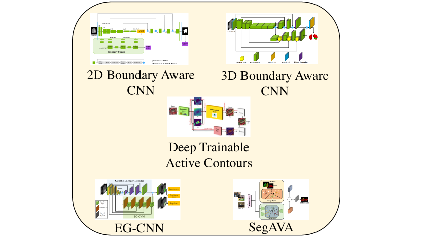
Figure 1: In this thesis, we introduce 2D and 3D edge-aware CNNs (EG-CNN) for segmentation, Deep Trainable Active Contours (DTAC) for segmentation with highly accurate boundaries, and segmentation with aligned variational autoencoder (SegAVA) that can learn from small datasets.

The goals of this thesis include devising novel deep learning models, which are illustrated in Figure 1, capable of learning powerful image representations, even with small datasets, that can be leveraged to yield highly accurate segmentation predictions and precisely delineate object and region boundaries. In the remainder of this chapter, we discuss these issues in greater detail and preview our solutions to some of these problems, which comprise the technical contributions of this thesis.

1 Edge-Aware Segmentation Networks

Intensity edges and textures contribute different information to image understanding. Edges (and boundaries) encode shape information, while textures determine the appearance of regions. FCNs have proven to be effective at representing and classifying textural information, thus transforming image intensity into output class masks that achieve semantic segmentation. In particular, the seminal U-Net architecture [102] demonstrated the effectiveness of down-sampling and up-sampling paths for multi-scale feature representation learning, and many encoder-decoder CNNs have since been introduced based on the same principles.

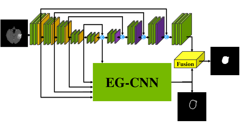
Figure 2: We propose a plug-and-play EG-CNN module that can be employed with any existing encoder-decoder backbone to increase the segmentation accuracy by supervising the edges.

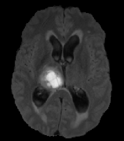
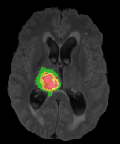
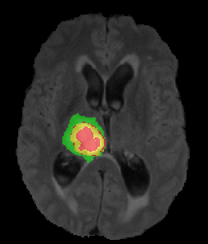
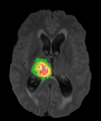
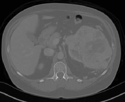
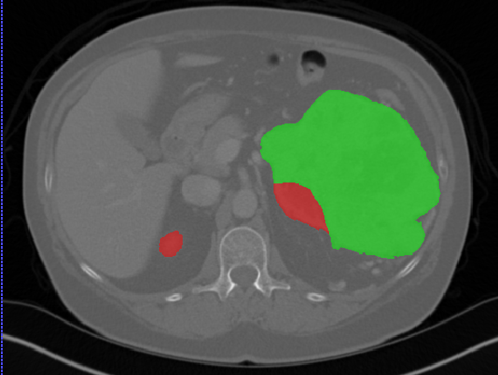
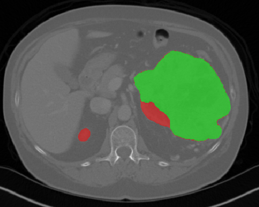
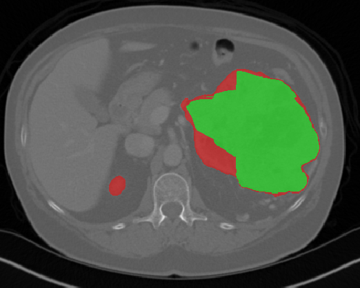
(a) Input images (b) Semantic Labels (c) Seg-Net+EG-CNN (d) Seg-Net

Figure 3: Visualization of segmentation outputs when our proposed EG-CNN is employed along with Seg-Net for the tasks of brain and kidney tumor segmentation in BraTS and KiTS datasets. EG-CNN improves the segmentation accuracy by effectively accounting for edge representations.

Geirhos et al. [35] empirically demonstrated that common CNN architectures are biased towards recognizing textures in the image, not object shape representations. This is in contrast to how humans normally segment images. In medical imaging for instance, expert manual segmentation often relies on the boundaries of anatomical structures; for example, to manually segment a liver, a medical practitioner usually identifies intensity edges first and subsequently fills the interior region in the segmentation mask. CNNs, which predominantly learn texture abstractions, often yield imprecise boundary delineations. Thus, CNN predictions often need to be post-processed to compensate for the shape details that the model fails to learn during training.

We argue that the sub-optimal paradigm of processing different abstractions within a single CNN pipeline can be remedied through the effective processing of information in a structured manner. Consequently, we devise strategies for disentangling the edge and texture information within a single training pipeline. Figure 2 illustrates how our proposed module, dubbed EG-CNN, can be paired with any existing CNN encoder-decoder to improve segmentation quality near intensity edges. We have applied our EG-CNN to the tasks of brain and liver tumor segmentation in medical images (Figure 3).

2 End-to-End Trainable ACMs

(1) Brain MR (2) Liver MR (3) Liver CT (4) Lung CT

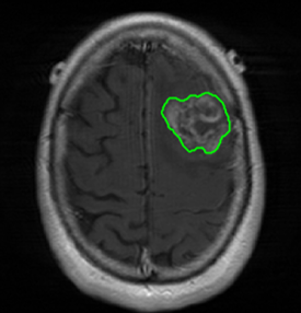
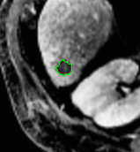
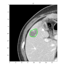
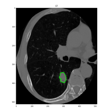
(a) Expert Manual

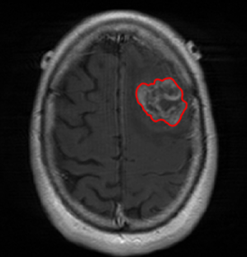
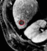
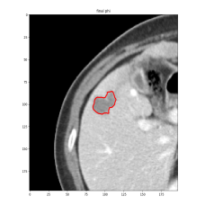
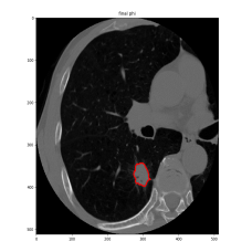
(b) DALS Output

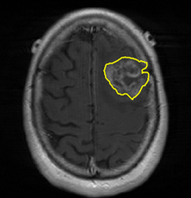
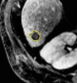
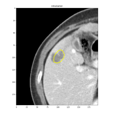
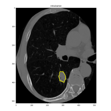
(c) U-Net Output

Figure 4: Segmentation comparison of (a) medical expert manual with (b) our DALS and (c) U-Net [102], in (1) Brain MR, (2) Liver MR, (3) Liver CT, and (4) Lung CT images.

Despite attempts to disentangle texture and edge information within a single pipeline, accurately delineating object boundaries remains a challenging task even for the most promising CNN architectures [20; 51; 137] that have achieved state-of-the-art performance on benchmark datasets (see also Appendix 7). The recently proposed Deeplabv3+ [22] mitigates this problem to some extent by leveraging dilated convolutions, but such improvements were made possible by extensive pre-training consuming vast computational resources.

Unlike CNNs that rely on large annotated datasets, massive computation, and hours of training, conventional ACMs are non-learning-based segmentation models that rely mainly on the content of the input image itself. ACMs have been successfully employed in various image analysis tasks, including object segmentation and tracking. In most ACM variants, the deformable curve(s) of interest dynamically evolves by an iterative process that minimizes an associated energy functional. However, the classic ACM [67] relies on some degree of user interaction to specify the initial contour and tune the parameters of the energy functional, which undermines its applicability to the automated analysis of large quantities of images.

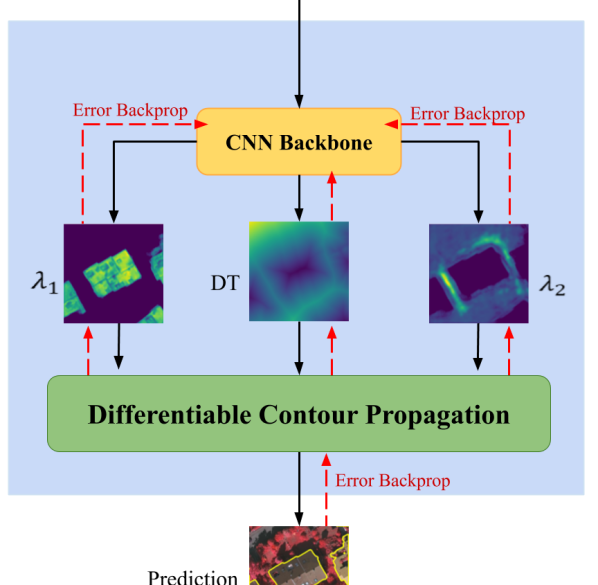
Figure 5: We propose a unified ACM-CNN framework that is automatically differentiable, hence end-to-end trainable without user supervision. The backbone CNN learns to initialize the ACM, via a generalized distance transform, and tune the per-pixel parameter maps in the ACM’s energy functional.

We first introduce a method for connecting the output of a CNN to an ACM, yielding a model for the precise delineation of lesions, to which we refer as Deep Active Lesion Segmentation (DALS) (Figure 4). We then go further to introduce a truly unified framework (Figure 5) that bridges the gap between ACMs and CNNs by leveraging a novel, automatically differentiable level-set ACM with trainable parameters that allows for back-propagation of gradients and can be end-to-end trained along with a backbone CNN from scratch, without any CNN pre-training. The ACM is initialized directly by the CNN and utilizes an energy functional that is locally-tunable by the backbone CNN, through 2D feature maps. Thus, our work overcomes the big hurdle of fully automating the powerful ACM approach to image segmentation. We have applied our proposed framework to the task of building segmentation in aerial images (Figure 6).

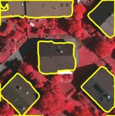
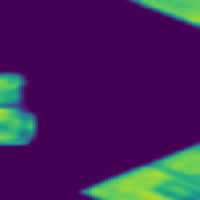
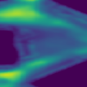
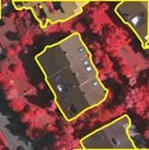
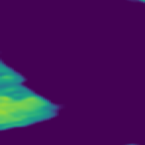
(a) Input image (b) DTAC Output (c) $\lambda_{1}(x,y)$ (d) $\lambda_{2}(x,y)$

Figure 6: Visualization of DTAC segmentation outputs and learned feature maps $\lambda_{1}(x,y)$ and $\lambda_{2}(x,y)$ used in DTAC’s energy functional.

3 Few-Shot Learning for Segmentation

In essence, CNNs and FCNs are hierarchical filter learning models in which the weights of the network are usually tuned by using a stochastic back-propagation error gradient decent optimization scheme. Since CNN architectures often include millions of trainable parameters, the training process is relies the sheer size of the dataset. Moreover, although fully-supervised models generally tend to perform better when given more training samples, they can still generalize poorly to unseen/novel classes not present in the training set.

For the task of semantic segmentation, establishing large-scale datasets with pixel-level annotations (that are not synthetic [64]) is time-consuming and prohibitively costly, and it may not be possible to include all possible classes in the training set. Although semi-supervised approaches aim to relax the level of supervision to bounding boxes and image-level tags, these models still require copious training samples and are prone to sub-optimal performance on unseen classes.

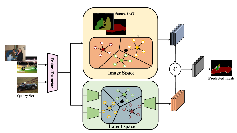
Figure 7: Overview of the SegAVA architecture for few-shot semantic segmentation.

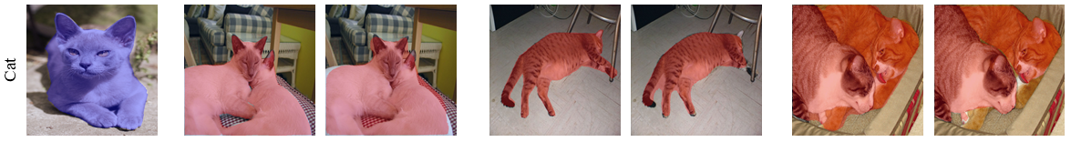
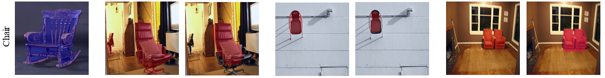
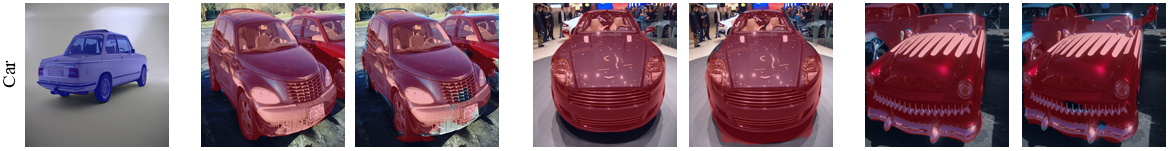
Figure 8: Example results from evaluating SegAVA in 1-way, 1-shot segmentation on the PASCAL-5i dataset.

By contrast, the few-shot learning [72] paradigm attempts to utilize a few annotated samples, referred to as “support samples”, to learn novel representations that belong to unseen classes, denoted as “query samples”. The few-shot learning paradigm was initially focused on image classification and later expanded to image segmentation [108; 30]. We propose a novel framework for few-shot image segmentation (Figure 7), which we call Segmentation with Aligned Variational Autoencoders (SegAVA), that explores the latent and image spaces of support and query sets to find the most common class-specific embeddings, and fuses them to produce the final semantic segmentation. We have applied SegAVA to the task of semantic segmentation of natural images (Figure 8).

4 Contributions

The specific contributions of this thesis are as follows:

1. Edge-Aware 2D Image Segmentation Networks
   [49; 48]: Fully convolutional neural networks (CNNs) have proven to be effective at representing and classifying textural information, thus transforming image intensity into output class masks that achieve semantic image segmentation. In medical image analysis, however, expert manual segmentation often relies on the boundaries of anatomical structures of interest. We propose 2D edge-aware CNNs for medical image segmentation. Our networks are designed to account for organ boundary information, both by providing a special network edge branch and edge-aware loss terms, and they are trainable end-to-end. We validate their effectiveness on the task of brain tumor segmentation using the BraTS 2018 dataset. Our experiments reveal that our approach yields more accurate segmentation results, which makes it promising for more extensive application to medical image segmentation.

2. Edge-Aware 3D Image Segmentation Networks
   [91]: Automated segmentation of kidneys and kidney tumors is an important step in quantifying the tumor’s morphometrical details to monitor the progression of the disease and accurately compare decisions regarding the kidney tumor treatment. Manual delineation techniques are often tedious, error-prone and require expert knowledge for creating unambiguous representation of kidneys and kidney tumors segmentation. We propose a 3D end-to-end edge-aware FCN for reliable kidney and kidney tumor semantic segmentation from arterial phase abdominal 3D CT scans. Our segmentation network consists of an encoder-decoder architecture that specifically accounts for organ and tumor semantics. We evaluate our model on the 2019 MICCAI KiTS Kidney Tumor Segmentation Challenge dataset.

3. Plug-and-Play Edge-gated 3D Image Segmentation Networks
   [50]: We propose a plug-and-play module, dubbed Edge-Gated CNNs (EG-CNNs), that can be used with existing encoder-decoder architectures to process both edge and texture information. The EG-CNN learns to emphasize the edges in the encoder, to predict crisp boundaries by an auxiliary edge supervision, and to fuse its output with the original CNN output. We evaluate the effectiveness of the EG-CNN against various mainstream CNNs on the publicly available BraTS19 dataset for brain tumor semantic segmentation, and demonstrate how the addition of EG-CNN consistently improves segmentation accuracy and generalization performance.

4. Deep Active Lesion Segmentation
   [45]: Lesion segmentation is an important problem in computer-assisted diagnosis that remains challenging due to the prevalence of low contrast, irregular boundaries that are unamenable to shape priors. We introduce Deep Active Lesion Segmentation (DALS), a fully automated segmentation framework that leverages the powerful nonlinear feature extraction abilities of FCNs and the precise boundary delineation abilities of ACMs. Our DALS framework benefits from an improved level-set ACM formulation with a per-pixel-parameterized energy functional and a novel multiscale encoder-decoder CNN that learns an initialization probability map along with parameter maps for the ACM. We evaluate our lesion segmentation model on a new Multiorgan Lesion Segmentation (MLS) dataset that contains images of various organs, including brain, liver, and lung, across different imaging modalities—MR and CT. Our results demonstrate favorable performance compared to competing methods, especially for small training datasets.

5. End-to-End Trainable Deep Active Contour Models
   [47]: The automated segmentation of buildings in aerial images is an important task in many applications, which requires the accurate delineation of multiple building instances of interest over a typically large area of pixel space. Manual methods are often laborious and current deep learning approaches typically suffer from inaccurate delineation of segmented instances. We introduce Deep Trainable Active Contours (DTAC), an end-to-end trainable image segmentation framework that unifies a CNN and a differentiable localized ACM with learnable parameters for fast and robust delineation of buildings in satellite imagery. The ACM’s Eulerian energy functional includes per-pixel parameter maps predicted by the backbone CNN, which also initializes the ACM. Importantly, both the CNN and ACM components are fully implemented in TensorFlow, and the entire DTAC architecture is end-to-end automatically differentiable and backpropagation trainable without user intervention. Unlike earlier efforts employing Lagrangian ACMs for building segmentation, our DTAC enables the fast and fully automated simultaneous delineation of arbitrarily many instances of buildings. We validate our model on two publicly available aerial image datasets for building segmentation (Vaihingen and Bing Huts), and our results demonstrate that DTAC establishes a new state-of-the-art performance.

6. Few-Shot Semantic Segmentation: We address the challenging problem of few-shot image segmentation by feature alignment in the image and latent spaces of support and query samples. Our model, which is dubbed SegAVA, leverages a latent stream as well as an encoder-decoder stream to extract the most essential discriminative semantic embeddings and learn similarities in both spaces. The latent stream consists of two variational autoencoders, conditioned on support and query sets, that jointly learn to generate the input images and discriminatively identify the most common class-specific representations using a Wasserstein-2 metric. These embedding are then decoded to the image space and concatenated into a common representation found by comparing support and query extracted features using our fully convolutional decoder. We train and test our SegAVA model using the PASCAL-5i dataset, and our results demonstrate new state-of-the-art performance in 1-shot and 5-shot scenarios. We also validate the SegAVA model in a semi-supervised setting where only bounding boxes are provided, and the results demonstrate the effectiveness of our approach.

5 Overview

The remainder of the thesis is organized as follows:

In Chapter 1, we review the relevant literature in the area of edge-aware CNN networks that utilize edge and texture information in a specialized manner, hybrid frameworks that leverage ACMs and CNNs within a single segmentation pipeline, and few-shot learning with an emphasis on semantic image segmentation.

In Chapter 2, we propose an end-to-end edge-aware network that processes texture and edge information in dedicated branches, the latter supervised with edge-aware loss functions. Additionally, we propose EG-CNN, which is a plug-and-play, volumetric (3D) segmentation module that can be paired with any existing volumetric CNN architecture so as to disentangle texture and edge processing and improve the segmentation accuracy near intensity edges.

In Chapter 3, we propose DTAC, an end-to-end trainable image segmentation framework that unifies ACMs and CNNs, resulting in a differentiable ACMs with learnable parameters for fast and robust segmentation and delineation.

In Chapter 4, we propose SegAVA, an end-to-end, few-shot segmentation framework that leverages a latent stream as well as an encoder-decoder stream to extract the most essential discriminative semantic embeddings and learn similarities in both spaces and efficiently segment images, given only a handful of labeled examples.

In Chapter 5, we describe our experiments with the models developed in the previous chapters and benchmark our results.

Chapter 6 presents the conclusions of the thesis and suggests promising future research directions.

Appendix 7 presents a novel deep learning-based methodology for 3D human lung lobe segmentation.

Chapter 1 Related Work

In this chapter, we first review the relevant research focusing on image segmentation using FCNs. We then review efforts at designing networks that are more aware of boundaries, as well efforts to combine ACMs and CNNs. Finally, we review relevant work in few-shot learning and, in particular, few-shot image segmentation.

1 Fully Convolutional Networks for Image Segmentation

1 Natural Image Segmentation

Long et al. [82] introduced fully convolutional neural networks (Figure 1(a)) for semantic segmentation, interleaving convolutional and pooling layers to learn the combined semantic and appearance information, eventually generating per-pixel prediction maps wherein boundaries were often blurred due to the reduction of resolution. Liu et al. [80] proposed a global context module (Figure 1(b)) that alleviated the issue of local confusion.

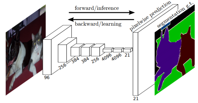
(a)

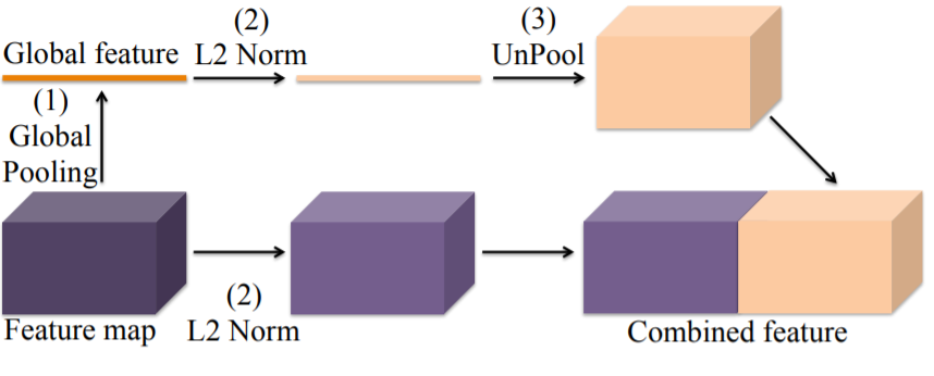
(b)

Figure 1: (a) Architecture of FCNs for image segmentation. (b) Architecture of the ParsNet context module. Images from [19], [95], and [6].

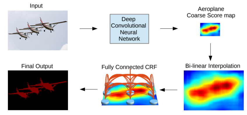
(a)

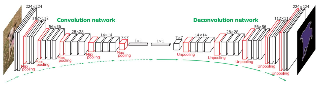
(b)

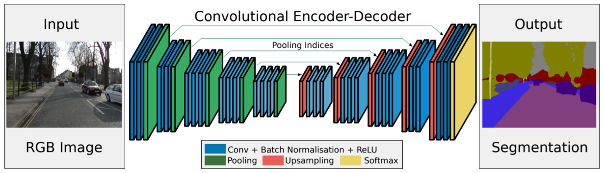
(c)

Figure 2: (a) Overview of DeepLab. (b) Architecture of deconvolutional network. (C) Architecture of SegNet. Images from [82] and [80].

Furthermore, Chen et al. [19] proposed to combine the output of the last layer of a CNN with a fully connected Conditional Random Field (CRF) in order to overcome the poor localization property of CNNs. Their model, which they called DeepLab (Figure 2(a)), achieved significantly better segmentation predictions near edges due to the ability of CRFs to fully delineate mis-segmented regions. One of the early efforts that utilized an encoder-decoder-like architecture for semantic segmentation is by Noh et al. [95], where a decoding network consisting of deconvolutional and unpooling layers was added to a VGG16 backbone [113] for predicting pixel-wise outputs (Figure 2(b)). Following this work, Badrinarayanan et al. [6] proposed to use an encoder-decoder architecture (Figure 2(c)), without the VGG16 backbone, where the low-resolution, encoded feature maps are decoded back up to the original input image resolution.

A follow-up effort by Chen et al. [20], called DeepLabv2, extended this DeepLab framework by leveraging the power of dilated convolutional layers to explicitly control the resolution of the feature responses and enlarge the field of view of filters without additional free parameters. In addition, this work introduced a novel module, dubbed Dilated Spatial Pyramid Pooling (DSPP), which enabled accurate segmentation at multiple resolutions.

The use of multi-scale information for semantic segmentation has also been explored by various researchers and shown to be effective. Yu and Koltun [131] proposed an architecture that uses dilated convolutions in order to increase the receptive fields in an efficient manner while aggregating multi-scale semantic information. Zhao et al. [137] introduced the pyramid scene parsing network (PSPNet) (Figure 3(a)), which extracted and aggregated global context information and improved the quality of segmentation without employing computationally expensive post processing methods like the CRF used in [19].

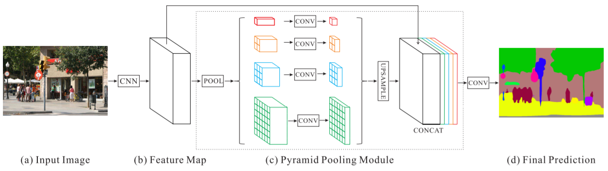
(a)

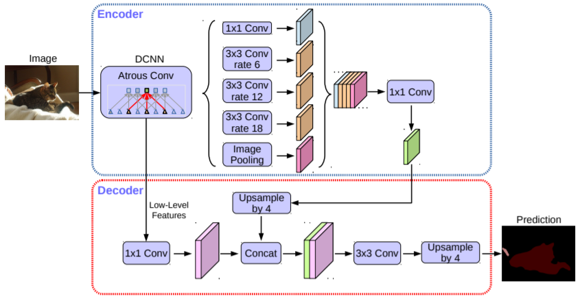
(b)

Figure 3: (a) Architecture of the PSPNet. (b) Architecture of DeepLabv3+. Images from [137] and [22].

DeepLabv3 [21] attempted to capture multi-scale context by using multiple dilation rates in cascaded and DSPP modules that leveraged dilated convolutions. Furthermore, DeepLabv3+ [22] (Figure 3(b)) employed an architecture similar to DeepLabv3 [21], but proposed the use of an decoder network to improve segmentation accuracy around edges. In DeepLabv3+, depthwise separable convolutional layers were used in both the DSPP module and decoder network and reportedly improved the computational performance.

2 Medical Image Segmentation

A seminal paper in deep learning applied to medical image segmentation is that by Ronneberger et al. [102], which introduces a 2D FCN comprising an encoder and decoder that are connected by skip connections at different resolutions. This work was later extended [26] to 3D segmentation. Milletari et al. [87] proposed an encoder-decoder architecture with residual blocks, denoted as V-Net, for volumetric medical image segmentation. Gibson et al. [37] expanded the V-Net work by introducing dense feature blocks in the encoder network. Myronenko [90] applied an asymmetric encoder-decoder architecture with residual blocks to 3D brain tumor segmentation.

Variants of the U-Net encoder-decoder architecture have been proposed for various applications. Li et al. [77] introduced a hybrid architecture consisting of 2D and 3D U-Nets with dense blocks for the task of liver segmentation. Jin et al. [65] proposed a 2D U-Net architecture with deformable convolutions for the task of retinal vessel segmentation. For this segmentation task, [46; 44] proposed an encoder-decoder architecture that leverages dilated spatial pyramid pooling with multiple dilation rates to recover the lost content in the encoder and add multiscale contextual information to the decoder.

2 Edge-Aware Networks for Image Segmentation

This section separately reviews relevant literature on natural image segmentation and additional literature on medical image segmentation.

1 Natural Image Segmentation

Since the advent of deep learning, several efforts have been dedicated in particular to edge prediction and enhancing the quality of boundaries in the segmented areas. Yu et al. [132] proposed a multi-label semantic boundary detection network to improve a wide variety of vision tasks by predicting edges directly. They included a new skip-layer architecture in which category-wise edge activations at the top convolution layer share and are fused with the same set of bottom layer features, along with a multi-label loss function to supervise the fused activations.

Yu et al. [133] proposed a category-aware semantic edge detection framework in which direct predictions of edges improved a wide variety of vision tasks. Their method includes a skip-layer CNN architecture in which category-wise edge activations of the top and bottom convolution layers are shared and fused together. In addition, Yu et al. [134] demonstrated the vulnerability of CNNs to misaligned edge labels and proposed a framework for the simultaneous alignment and learning of the edges.

For the task of portrait image segmentation, Chen et al. [23] proposed a lightweight 2D encoder-decoder architecture with an added branch, consisting of boundary feature mining for selectively extracting detailed information of boundaries from the output segmentation of the CNN. Aiming to learn semantic boundaries, Hu et al. [57] presented a framework that aggregates different tasks of object detection, semantic segmentation, and instance edge detection into a single holistic network with multiple branches, demonstrating significant improvements over conventional approaches through end-to-end training.

Acuna et al. [2] predicted object edges by identifying pixels that belong to class boundaries, proposing a new layer and a loss that enforces the detector to predict a maximum response along the normal direction at an edge, while also regularizing its direction. Takikawa et al. [118] proposed a framework for semantic instance segmentation of objects in the Cityscapes dataset [27] in which such gates are employed to remove the noise from higher-level activations and process the relevant boundary-related information separately.

2 Medical Image Segmentation

An early model for medical image segmentation with an emphasis on edge learning is DCAN [18], in which the output of the decoder is also branched to learn the edges. However, DCAN does not prioritize such a learning scheme in a dedicated path and fusion simply amounts to the concatenation of the learned feature maps to the output of the main CNN. Consequently, this approach does not generalize well to more sophisticated segmentation tasks with irregular shapes. Subsequently, the CIA-Net [138] was introduced to address some of these issues by incorporating a more sophisticated fusion module.

For the application of 2D brain tumor segmentation, Shen et al. [109] proposed the use of separate decoders for learning the edges and tumor regions and concatenated the probability outputs of each before feeding them into two consecutive convolutional layers and a final softmax function. However, no specialized loss functions were designated for the edge predictions and utilizing replicated decoders with no effective connections is inefficient.

Murugesan et al. [89] introduced a edge-aware joint multi-task framework for medical image segmentation that utilizes parallel decoders, along with the main encoder-decoder stream, to perform contour prediction and distance map estimation. The proposed effort uses the same encoder for three parallel decoder streams, but does not utilize the predicted contour and distance map in making the final prediction.

Zhang et al. [136] use a 2D edge attention guidance network to learn the edge attention representation in the earlier stages of the encoding process and transfer them to multi-scale decoding layers where they are fused with the main encoder-decoder prediction using a weighted aggregation module.

Kidney and Kidney Tumor Segmentation

Kidney cancer accounted for nearly 175,000 deaths worldwide in 2018 [13], and it is projected that 14,770 deaths will occur due to the disease in 2019 in the US [111]. Current kidney tumor treatment planning includes Radical Nephrectomy (RN) and Partial Nephrectomy (PN). In RN, both the tumor and the affected kidney are removed whereas in PN the tumor is removed but kidneys are saved [116]. Although RNs were historically prevalent as a standard treatment procedure for kidney tumors, new capabilities for earlier detection of the tumors as well as advancements in surgery has made PNs a viable treatment approach [53].

Traditionally, various techniques such as deformable models [86], GrabCuts, region growing and atlas-based methods have been applied to the problem of kidney segmentation. In recent years, researchers have attempted to leverage the power of deep learning and CNNs to build segmentation frameworks that are more automated and less dependant on incorporation of prior shape statistics. Thong et al. [119] proposed a 2D patch-based approach for kidney segmentation in contrast-enhanced CT scans by leveraging a modified ConvNet.

Jackson et al. [62] developed a framework for detection and segmentation and of kidneys in non-contrast CT images by utilizing a 3D U-Net. Yang et al. [128] proposed a method for kidney and renal tumor segmentation in CT angiography images by a modified residual FCN that is equipped with a pyramid pooling module. Furthermore, Yin et al. [130] employed a cascaded approach for segmentation of kidneys with renal cell carcinoma by training a CNN that predicts a bounding box around the kidney and a subsequent CNN that segments the kidneys. Recently, Xia et al. [126] proposed a two-stage approach for the segmentation of kidney and space-occupying lesion areas by using SCNN and ResNet for image retrieval and SIFT-flow and MRF for smoothing and pixel matching.

3 End-to-End Trainable Deep Active Contours

In this section, we first present relevant work on ACMs with an emphasis on level-set ACMs. We then present a review of notable FCNs for 2D image segmentation including approaches used for building image segmentation. Finally, we review efforts that have attempted to combine ACMs and CNNs within a segmentation pipeline.

1 Level-Set ACMs

Eulerian active contours evolve the segmentation curve by dynamically propagating the zero level set of an implicit function so as to minimize a corresponding functional [97]. Level-set ACM segmentation requires determining suitable parameter values for the associated Partial Differential Equation (PDE), usually in a tedious trial and error process where each parameter value is tested over a series of images and remains the same for the entire image set. New images with different statistics typically require re-tuning of the parameters. Moreover, for images with diverse spatial statistics, a fixed set of parameters may result in suboptimal segmentation performance over all the images. Spatially adaptive parameters are better suited to accurate segmentation.

Most notable approaches that utilize this formulation are active contours without edges [17] and geodesic active contours [16]. The Caselles-Kimmel-Sapiro model is mainly dependent on the location of the level-set, whereas the Chan-Vese model mainly relies on the content difference between the interior and exterior of the level-set. In addition, Lankton and Tannenbaum [73] reformulate the Chan-Vese model such that the energy functional incorporates image properties in local regions around the level-set, and it was shown to more accurately segment objects with heterogeneous features.

Oliveira et al. [96] present a solution for liver segmentation based on a deformable model in which the parameters are adjusted via a genetic algorithm, but all the segmentations in their test set were obtained by using the same set of parameters. They and Baillard et al. [7] define the problem of parameter tuning as a classification of each point along the contour, performed by maximizing the posterior segmentation probability—if a point belongs to the object, then the implicit surface should locally extend, otherwise it should contract. However, only the direction of the curve evolution is considered, not its magnitude, which is critical especially in heterogeneous regions wherein convergence to local minima should be prevented.

Marquez-Neila et al. [84] proposed a morphological approach that approximates the numerical solution of the PDE by successive application of morphological operators defined on the equivalent binary level set. Hoogi et al. [54] presented an alternative, fully automatic model for the adaptive tuning of parameters, based on estimating the zero level set contour location relative to the lesion using the location probabilities, and showed significantly improved segmentations.

2 FCNs for Building Segmentation

An early effort in leveraging CNN-based models for building segmentation is by Audebert et al. [4] who used SegNet [6] with multi-kernel convolutional layers at three different resolutions. Subsequently, Wang et al. [123] proposed using ResNet [52], first to identify the instances, followed by an MRF to refine the predicted masks. Wu et al. [125] employed a U-Net encoder-decoder architecture with loss layers at different scales to progressively refine the segmentation masks. Xu et al. [127] proposed a cascaded approach in which pre-processed hand-crafted features are fed into a Residual U-Net to extract the building locations and a guided filter to refine the results.

Furthermore, Bischke et al. [10] proposed a cascaded multi-task loss function to simultaneously predict the semantic masks and distance classes in an effort to address the problem of poor boundary predictions by CNN models. Recently, Rudner et al. [105] proposed a method to segment flooded buildings using multiple streams of encoder-decoder architectures that extract spatiotemporal information from medium-resolution images and spatial information from high-resolution images along with a context aggregation module to effectively combine the learned feature map.

3 Deep Learning Assisted Active Contours

Hu et al. [55] proposed a model in which the network learns a level-set function for salient objects; however, the authors predefined a fixed weighting parameter $\lambda$, which will not be optimal for all cases in the analyzed set of images. In medical image analysis, the challenges are much more complex—variability between images is high, there are many low-contrast images, and noise is very common. Ngo et al. [93] proposed to combine deep belief networks with implicit ACMs for cardiac left ventricle segmentation; However, their approach requires additional prepossessing steps such as edge detection and needs user intervention for setting the ACM’s parameters.

Le et al. [76] proposed a framework in which level-set ACMs are implemented as RNNs for the task of semantic segmentation of natural images. There are 3 key differences between that effort and our proposed model: (1) our model does not reformulate ACMs as RNNs, which makes it more computationally efficient. (2) our model benefits from a novel locally-penalized energy functional, as opposed to constant weighted parameters. (3) our model has an entirely different pipeline—we employ a single CNN that is trained from scratch along with the ACM, as opposed to requiring two pre-trained CNN backbones.

Marcos et al. [83] proposed Deep Structured Active Contours (DSAC), an integration of ACMs with CNNs in a structured prediction framework for building instance segmentation in aerial images. There are 3 key differences between that work and our work: (1) our model is fully automated and runs without any external supervision, as opposed to depending heavily on the manual initialization of contours. (2) our model leverages the Eulerian ACM, which naturally segments multiple building instances simultaneously, as opposed to a parametric formulation that can handle only a single building at a time. (3) our approach fully automates the direct back-propagation of gradients through the entire DTAC framework due to its automatically differentiable ACM.

Cheng et al. [25] proposed the Deep Active Ray Network (DarNet) that uses polar coordinates instead of Euclidean coordinates, and rays to prevent the problem of self-intersection, and employs a computationally expensive multiple initialization scheme to improve the performance of the proposed model. Like DSAC, DarNet can handle only single instances of buildings due to its explicit formulation. Our approach is inherently different from DarNet, as (1) it uses an implicit ACM formulation that handles multiple building instances and (2) leverages a CNN to automatically and precisely initialize the implicit ACM.

Gur et al. [41] used an explicit ACM, represented by a neural renderer, along with a backbone encoder-decoder that predicts a shift map to efficiently evolve the contour via edge displacement.

Some efforts have also focused on deriving new loss functions that are inspired by ACM principles. Inspired by the global energy formulation of Chan and Vese [17], Chen et al. [24] proposed a supervised loss layer that incorporated area and size information of the predicted masks during training of a CNN and tackled the problem of ventricle segmentation in cardiac MRI. Similarly, Gur et al. [42] presented an unsupervised loss function based on morphological active contours without edges [84] for microvascular image segmentation.

4 Few-Shot Learning

1 Few-Shot Classification

In few-shot classification, the goal is to learn unseen classes given a few labeled training examples for each class. Among different approaches that have been proposed for this problem, metric-based methodologies [71; 114; 78] have grained the most traction. In such a paradigm, a metric function compares the similarity between the extracted features of labeled and unlabeled samples. Vinyals et al. [121] introduced Matching Networks, which consisted of a recurrent neural network and a cosine similarity metric function for one-shot classification tasks. Similarly, Snell et al. [114] presented a prototypical learning framework that used a Euclidean distance function as the learning metric.

In contrast to these approaches that utilize fixed-distance metrics, Sung et al. [117] used a convolutional neural network, denoted as Relation Network, to learn to learn a deep distance metric in an end-to-end manner. Garcia and Bruna [34] expanded this idea and used a graph convolutional neural network to learn the distance metric. Other approaches have also sought to utilize the latent space for learning the semantic embeddings. Kim et al. [68] introduced a variational prototype encoder in which a generalizable embedding latent space is learned for identifying novel categories. Schonfeld et al. [107] proposed to use a shared latent space to identify important multi-domain information for unseen categories.

2 Few-Shot Segmentation

Few-shot semantic segmentation extends the idea of few-shot learning to dense pixel-wise predictions. Shaban et al. [108] were the first to study the problem of 1-way semantic segmentation and used a conditional branch to learn the important embedding in the support set and combine it with query features in a separate branch to produce the final segmentation. Furthermore, Rakelly et al. [101] introduced a network that was conditional on the support set and performed inference on the query set via feature fusion. Hu et al. [56] proposed an attention mechanism to highlight multi-scale context features between support and query features and used a Conv-LSTM to fuse learned features.

In contrast to the approaches that separately processed support and query embeddings, Zhang et al. [135] used a masked average pooling scheme to create guidance features from support images and aggregated them with query features to obtain the final segmentation using a unified pipeline. In this work, cosine similarity was used to measure the distance between features in the support and query sets. Following this single-branch strategy, Siam et al. [110] proposed a multi-resolution adaptive imprinting to identify the similarities of extracted features.

Nguyen and Todorovic [94] computed a class feature vector as the average of foreground areas in the extracted support features and used it to compare against query features by a cosine similarity metric. In a similar approach, Wang et al. [122] employed a prototypical learning framework, PANet, in which support prototypes are extracted by a masked average pooling and compared against query prototypes by using the cosine similarity metric. Additionally, PANet uses a prototype alignment regularization by using the predicted query masks to further align the support and query embeddings.

Unlike earlier efforts, we utilize both latent and image spaces to find the most common class-specific representations for the task of few-shot semantic segmentation. Additionally, we introduce a fully convolutional decoder to learn the similarities in the image space. Our method achieves state-of-the-art results on the popular PASCAL-5i dataset [108] and effectively segments images using weaker levels of supervision, such as bounding boxes.

Chapter 2 Edge-Aware Semantic Segmentation Networks

In this chapter, we first introduce a 2D encoder-decoder architecture that leverages a special interconnected edge layer module that is supervised by edge-aware losses in order to preserve boundary information and emphasize it during training. By explicitly accounting for the edges, we encourage the network to internalize edge importance during training. Our method utilizes edge information only to assist training for semantic segmentation, not for the main purpose of predicting edges directly. This strategy enables a structured regularization mechanism for our network during training and results in more accurate and robust segmentation performance during inference.

Furthermore, we extend our methodology and propose 3D boundary-aware FCNs for end-to-end and reliable semantic segmentation of kidneys and kidney tumor by encoding the information of edges in a dedicated stream that is supervised by edge-aware losses.

Lastly, we create a 3D plug-and-play module that we call the Edge-Gated CNN (EG-CNN), which can be incorporated with any encoder-decoder architecture to disentangle the learning of texture and edge representations. The contribution of the proposed EG-CNN is two-fold. First, EG-CNN leverages an effective way to progressively learn to highlight the edge semantics from multiple scales of feature maps in the main encoder-decoder architecture by a novel and efficient layer denoted the edge-gated layer. Second, instead of separately supervising the edge and texture outputs, the EG-CNN uses a dual-task learning scheme, in which these representations are jointly learned by a consistency loss. Therefore, without increasing the cost of data annotation and by exploiting the duality between edge and texture predictions, the EG-CNN improves the overall segmentation performance with highly detailed boundaries.

1 2D Edge-Aware Encoder-Decoders

1 Architecture

Our network comprises a main encoder-decoder stream for semantic segmentation as well as a shape stream that processes the feature maps at the boundary level (Figure 1). In the encoder portion of the main stream, every resolution level includes two residual blocks whose outputs are fed to the corresponding resolution of the shape stream. A $1\times 1$ convolution is applied to each input to the shape stream and the result is fed into an attention layer that is discussed in the next section.

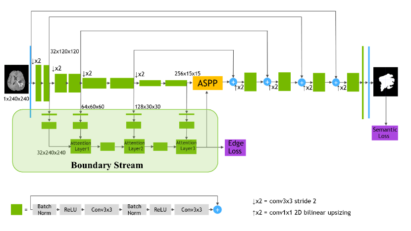
Figure 1: 2D fully convolutional edge-aware architecture.

The outputs of the first two attention layers are fed into connection residual blocks. The output of the last attention layer is concatenated with the output of the encoder in the main stream and fed into a dilated spatial pyramid pooling layer. Losses that contribute to tuning the weights of the model come from the output of the shape stream that is resized to the original image size, as well as the output of the main stream.

2 Attention Layer

Each attention layer receives inputs from the previous attention layer as well as the main stream at the corresponding resolution. Let $s_{l}$ and $m_{l}$ denote the attention layer and main stream layer inputs at resolution $l$. First, $s_{l}$ and $m_{l}$ are concatenated and a $1\times 1$ convolution layer $C_{1\times 1}$ is applied, followed by a sigmoid function $\sigma$, to obtain an attention map:

$$\alpha_{l}=\sigma\big{(}C_{1\times 1}(s_{l}\mathbin{\|}m_{l})\big{)}.$$ (1)

An element-wise multiplication is then performed with the input to the attention layer to obtain the output of the attention layer, denoted as

$$o_{l}=s_{l}\odot\alpha_{l}.$$ (2)

3 Edge-Aware Segmentation

Our network jointly learns the semantics and boundaries by supervising the output of the main stream as well as the edge stream. We use the generalized Dice loss on predicted outputs of the main stream and the shape stream. Additionally, we add a weighted binary cross entropy loss to the shape stream loss in order to deal with the large imbalance between the boundary and non-boundary pixels. The overall loss function of our network is

$$L_{\text{total}}=\lambda_{1}L_{\text{Dice}}(y_{\text{pred}},y_{\text{true}})+\lambda_{2}L_{\text{Dice}}(s_{\text{pred}},s_{\text{true}})+\lambda_{3}L_{\text{Edge}}(s_{\text{pred}},s_{\text{true}}),$$ (3)

where $y_{\text{pred}}$ and $y_{\text{true}}$ denote the pixel-wise semantic predictions of the main stream while $s_{\text{pred}}$ and $s_{\text{true}}$ denote the boundary predictions of the shape stream; $s_{\text{true}}$ can be obtained by computing the spatial gradient of $y_{\text{true}}$.

The Dice loss [87] in (3) is

$$L_{\text{Dice}}=1-\frac{2\sum y_{\text{true}}y_{\text{pred}}}{\sum y_{\text{true}}^{2}+\sum y_{\text{pred}}^{2}+\epsilon},$$ (4)

where summation is carried over the total number of pixels and $\epsilon$ is a small constant to prevent division by zero.

The edge loss in (3) is

$$L_{\text{Edge}}=-\beta\sum_{j\in y_{+}}\log P(y_{\text{pred},j}=1\mid x;\theta)-(1-\beta)\sum_{j\in y_{-}}\log P(y_{\text{pred},j}=0\mid x;\theta),$$ (5)

where $x$, $\theta$, $y_{-}$, and $y_{+}$ denote the input image, CNN parameters, and edge and non-edge pixel sets, respectively, $\beta$ is the ratio of non-edge pixels over the entire number of pixels, and $P(y_{\text{pred},j})$ denotes the probability of the predicated class at pixel $j$.

2 3D Edge-Aware Encoder-Decoders

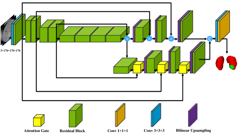
Figure 2: Proposed volumetric (3D) edge-aware architecture for kidney and kidney tumor segmentation.

1 Framework Architecture

As is illustrated in Figure 2, our network consists of the main segmentation branch and the additional boundary stream that processes the feature maps at the boundary level. The main branch, following [90], is an asymmetric encoder-decoder structure. The input to the encoder is a $176\times 176\times 176$ crop which is initially fed into a $3\times 3\times 3$ convolution with 16 filters. Feature maps are then extracted at each resolution by feeding them into a residual block followed by a strided $3\times 3\times 3$ convolution (for downsizing and doubling of the feature dimension).

The bottom of the encoder entails four consecutive residual blocks that are connected to the decoder. The extracted feature maps in the decoder are upsampled using bilinear interpolation and added with feature maps from the encoder. The output of the decoder is concatenated with the output of the boundary and fed into a $1\times 1\times 1$ convolution with 2 channels where channel-wise sigmoid activation $\sigma(X)=1/(1+e^{-X})$ determines the probability of each voxel belonging to kidneys and tumor or only tumor classes.

2 Boundary Stream

The purpose of the boundary stream is to highlight the edge information of the feature maps extracted in the main encoder by leveraging an additional attention-driven decoder. The attention gates in every resolution of the boundary stream process the feature maps that are learned in the main encoder as well as the output of the previous attention gates.

For the first attention gate, we first concatenate the output of the encoder with its previous resolution and feed it into a residual block. In the attention gates, each input is first fed into a $3\times 3\times 3$ convolutional layer with matching number of feature maps and then fused together, followed by ReLU. The output of the ReLU is fed into a $1\times 1\times 1$ convolution layer followed by sigmoid function $\sigma$ to obtain the attention map. Consecutively, an element-wise multiplication between the boundary stream feature maps and the computed attention map results in the output of the attention gates.

3 Loss Functions

We use a dice loss function on the predicted outputs of the main stream as well as the boundary stream. The dice loss is as follows [87]:

$$L_{\text{Dice}}=1-\frac{2\sum y_{\text{true}}\,y_{\text{pred}}}{\sum y_{\text{true}}^{2}+\sum y_{\text{pred}}^{2}+\epsilon},$$ (6)

where $y_{\text{pred}}$ and $y_{\text{true}}$ denote the voxel-wise semantic predictions of the main stream and their corresponding labels, $\epsilon$ is a small constant to avoid division by zero and summation is carried over the total number of voxels.

Additionally, we add a weighted Binary Cross Entropy (BCE) loss to the boundary stream loss in order to deal with the imbalanced number of boundary and non-boundary voxels:

$$L_{\text{BCE}}=-\beta\sum_{j\in y_{+}}\log P(y_{\text{pred},j}=1\mid x;\theta)-(1-\beta)\sum_{j\in y_{-}}\log P(y_{\text{pred},j}=0\mid x;\theta),$$ (7)

where $x$, $\theta$, $y_{-}$, and $y_{+}$ denote the 3D input image, CNN parameters, edge, and non-edge voxel sets, respectively, $\beta$ is the ratio of non-edge pixels over the entire number of voxels, and $P(y_{\text{pred},j})$ denotes the probability of the predicated class at voxel $j$.

The total loss function that is minimized during training is computed by taking the average of losses for tumor-only and foreground class predictions.

3 Plug-and-Play Edge-Aware CNNs (EG-CNNs)

We next present a plug-and-play edge-aware CNN, dubbed EG-CNN, and introduce its architecture. The main stream, a generic CNN encoder-decoder, learns feature representations that span multiple resolutions. Our EG-CNN receives each of the feature maps in the main stream and learns to highlight the edge representations. In particular, the EG-CNN consists of a sequence of residual blocks followed by tailored layers, as we denote the edge-gated layers, to progressively extract the edge representations.

The output of the EG-CNN is then concatenated with the output of the main stream in order to produce the final segmentation output. Furthermore, the main stream and the EG-CNN are supervised by their own dedicated loss layers as well as a consistent loss function that jointly learns the output of both streams. The edge ground-truth is generated online by applying a 3D Sobel filter to the original ground truth masks.

Each edge-gated layer requires two inputs that originate from the main stream and the EG-CNN stream. The intermediate feature maps from every resolution of the main stream as well as the first up-sampled feature maps in the decoder are fed to the EG-CNN as inputs.

The latter is first fed into a residual block followed by bilinear upsampling before being fed into the edge-gated layer along with the input from its previous resolution in the encoder. The output of each edge-gated layer (except for the last one) is fed into another residual block followed by bilinear upsampling before being fed to the next edge-gated layer along with its corresponding input from the encoder (Figure 3).

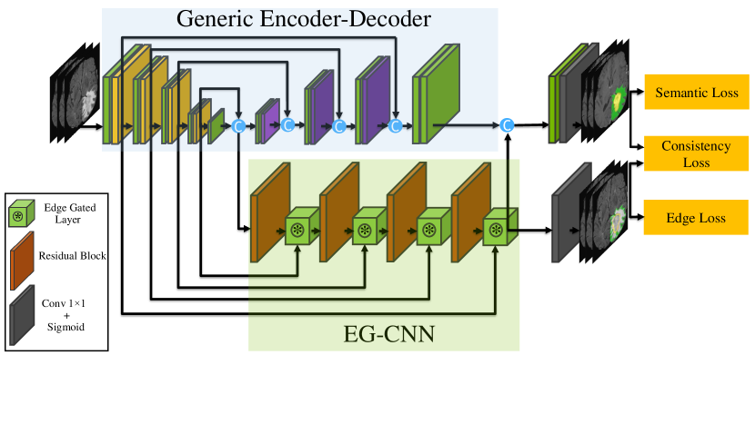
Figure 3: The EG-CNN module can be integrated with any generic encoder-decoder architecture and highlight the edge representations of the intermediate feature maps.

1 Edge-Gated Layer

Edge-gated layers highlight the edge features and connect the feature maps learned in the main and edge streams. They receive inputs from the previous edge-gated layers as well as the main stream at its corresponding resolution. Let $e_{r,in}$ and $m_{r}$ denote the inputs coming from edge and main streams, respectively, at resolution $r$. First, an attention map, $\alpha_{r}$ is obtained by feeding each input into a $1\times 1\times 1$ convolutional layer, $C_{1\times 1\times 1}$, fusing the outputs and passing them into a rectified linear unit (ReLU) $Re(X)=\max(0,X)$ according to

$$\alpha_{r}=\sigma\big{(}Re(C_{1\times 1\times 1}(e_{r,in})+C_{1\times 1\times 1}(m_{r}))).$$ (8)

The obtained attention map $\alpha_{r}$ is then pixel-wise multiplied by $e_{r,in}$ and fed into a residual layer with kernel $w_{r}$. Therefore, the output of each resolution in EG-CNN ,$e_{r,out}$, can be represented as

$$e_{r,out}=e_{r,in}\odot\alpha_{r}+e_{r,in}.$$ (9)

The computed attention map highlights the edge semantics that are embedded in the main stream feature maps. In general, there will be as many edge-gated layers as the number of different resolutions in the main encoder-decoder CNN architecture.

2 Loss Functions

The total loss of the EG-CNN is as follows:

$$L_{\text{Tot}}=L_{\text{Semantic}}+L_{\text{Consistency}}+L_{\text{Edge}},$$ (10)

where $L_{\text{Semantic}}$ represent standard loss functions used for supervising the main stream in a semantic segmentation network, $L_{\text{Edge}}$ represent tailored losses for learning the edge representations, and $L_{\text{Consistency}}$ is a dual-task loss for the joint learning of edge and texture and enforces the class consistency of predictions.

Semantic Loss:

Without loss of generality, we use the Dice loss [87] for learning the semantic representations of texture according to

$$L_{\text{Dice}}=1-\frac{2\sum y_{\text{true}}y_{\text{pred}}}{\sum y_{\text{true}}^{2}+\sum y_{\text{pred}}^{2}+\epsilon},$$ (11)

where summation is carried over the total number of pixels, $y_{\text{pred}}$ and $y_{\text{true}}$ denote the pixel-wise semantic predictions of the main stream, and $\epsilon$ is a small constant to prevent division by zero.

Edge Loss:

The edge loss used in EG-CNN comprises of Dice loss [87] and balanced cross entropy [133], as follows:

$$L_{\text{Edge}}=\lambda_{1}L_{\text{Dice}}+\lambda_{2}L_{\text{BCE}},$$ (12)

where $\lambda_{1}$ and $\lambda_{2}$ are hyper-parameters. Let $e_{\text{pred},j}$ and $e_{\text{true},j}$ denote the edge prediction outputs of the EG-CNN and its corresponding groundtruth at voxel $j$, respectively. Then the balanced cross entropy $L_{\text{BCE}}$ used in (12) can be defined as

$$L_{\text{BCE}}=-\beta\sum_{j\in e_{+}}\log P(e_{\text{pred},j}=1\mid x;\theta)-(1-\beta)\sum_{j\in e_{-}}\log P(e_{\text{pred},j}=0\mid x;\theta),$$ (13)

where $x$, $\theta$, $e_{-}$, and $e_{+}$ denote the input image, CNN parameters, edge, and non-edge voxel sets, respectively, $\beta$ is the ratio of non-edge voxels to all voxels, and $P(e_{\text{pred},j})$ is the probability of the predicated class at voxel $j$. The cross entropy loss follows (13) except for the fact that non-edge voxels are not weighted.

Consistency Loss:

We exploit the duality of edge and texture predictions and simultaneously supervise the outputs of the edge and main stream by the consistency loss. Inspired by [118], the semantic probability predictions of the main CNN architectures and the ground truth masks are first converted into edge predictions by taking the spatial derivative in a differentiable manner. Subsequently, we penalize the mismatch between the boundary predictions of the semantic masks and the corresponding ground truth by utilizing an $L_{1}$ loss. Let $y_{\text{pred},j}$ denote the output of the main stream and $c$ represent the segmentation class. We propose a consistency loss function

$$L_{\text{Consistency}}=\sum_{j\in e_{+}}\bigl{(}\|{\nabla(\operatorname*{arg\,max}(P(y_{\text{pred},j}=1\mid e;c))}\|)-\|{\nabla(y_{\text{true},j}}\|\bigr{)}.$$ (14)

Due to the non-differentiability of the $\operatorname*{arg\,max}$ function, we leverage the Gumbel softmax trick [63] to avoid blocking the error-gradient. Thus, the gradient of the $\operatorname*{arg\,max}$ can be approximated according to

$$\frac{\partial\operatorname*{arg\,max}_{t}P(y^{t})}{\partial\gamma_{j}}=\nabla_{j}\frac{e^{(\log P(y_{t})+g_{t})/\tau}}{\sum_{i}e^{(\log P(y_{i})+g_{i})/\tau}},$$ (15)

where $\gamma$ is a differentiation dummy variable, $\tau$ is the temperature, set as a hyper-parameter, and $g_{i}$ denotes the Gumbel density function.

Chapter 3 End-to-End Trainable Deep Active Contour Models

ACMs [67] have been extensively applied to computer vision tasks such as image segmentation, especially for medical image analysis [86]. ACMs leverage parametric (“snake”) or implicit (level-set) formulations in which the contour evolves by minimizing an associated energy functional, typically using a gradient descent procedure. In the level-set formulation, this amounts to solving a PDE to evolve object boundaries that are able to handle large shape variations, topological changes, and intensity inhomogeneities. Alternative approaches to image segmentation that are based on deep learning have recently been gaining in popularity. CNNs can perform well in segmenting images within datasets on which they have been trained, but they may lack robustness when cross-validated on other datasets. Moreover, in medical image segmentation, CNNs tend to be less precise in boundary delineation than ACMs.

In this chapter, we establish a modeling framework that benefits from data-driven non-linear feature extraction capabilities of CNNs and versatility of ACMs. In essence, our goal is to employ a backbone CNN for initializing and guiding the ACM in a fully automated manner and without any user interaction.

First, we introduce a fully automatic framework for medical image segmentation that combines the strengths of CNNs and level-set ACMs to overcome their respective weaknesses. We apply our proposed Deep Active Lesion Segmentation (DALS) framework to the challenging problem of segmenting lesions in MR and CT medical images, dealing with lesions of substantially different sizes within a single framework. In particular, our proposed encoder-decoder architecture learns to localize the lesion and generates an initial attention map along with associated parameter maps, thus instantiating a level-set ACM in which every location on the contour has local parameter values.

By automatically initializing and tuning the segmentation process of the level-set ACM, our DALS yields significantly more accurate boundaries in comparison to conventional CNNs and can reliably segment lesions of various sizes.

Furthermore, we combine CNNs and ACMs in an end-to-end trainable framework that leverages an automatically differentiable ACM with trainable parameters. By enabling the backpropagation of gradients for stochastic optimization, the ACM and a backbone CNN can be trained together from scratch, without pre-training. Moreover, our ACM utilizes a locally-penalized energy functional that is directly predicted by its backbone CNN, through 2D feature maps, and it is initialized directly by the CNN. Thus, our work alleviates the biggest obstacle to exploiting the power of ACMs—eliminating the need for any type of user supervision or intervention.

1 Level-Set Active Contour Model With Parameter Functions

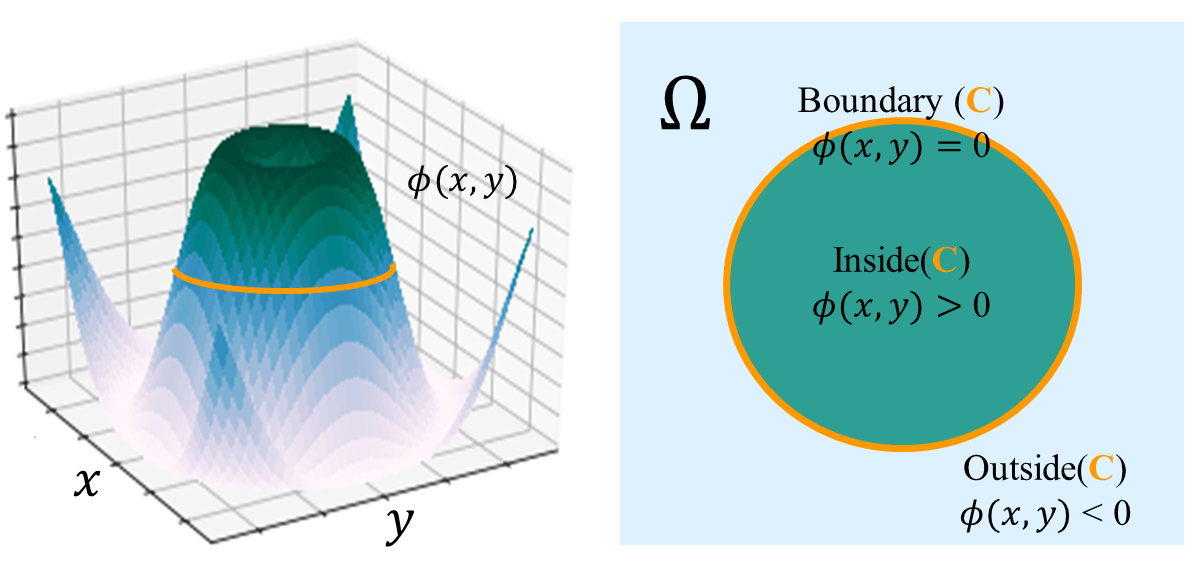
Figure 1: Boundary $C$ represented as the zero level set of implicit function $\phi(x,y)$.

First proposed by Osher and Sethian [98] to evolve wavefronts in CFD simulations, a level-set is an implicit representation of a hypersurface that is dynamically evolved according to the nonlinear Hamilton-Jacobi equation. Similarly, instead of working with a parametric contour that encloses the desired area to be segmented, we represent the contour as the zero level set of an implicit function. Let $I$ represent an input image and $C=\big{\{}(x,y)\mid\phi(x,y)=0\big{\}}$ be a closed contour in $\Omega\in R^{2}$ represented by the zero level set of the signed distance map $\phi(x,y)$ (Figure 1). The interior and exterior of $C$ are represented by $\phi(x,y)>0$ and $\phi(x,y)<0$, respectively. Following [17], we use a smoothed Heaviside function $H$ to represent the interior $(H(\phi))$ and exterior $(1-H(\phi))$ according to

$$H(\phi(x,y))=\frac{1}{2}+\frac{1}{\pi}\arctan\Big{(}\frac{{\phi(x,y)}}{\epsilon}\Big{)}.$$ (1)

The derivative of $H(\phi(x,y))$ is

$$\delta\phi(x,y)=\frac{\partial H(\phi(x,y))}{\partial\phi(x,y)}=\frac{1}{\pi}\frac{\epsilon}{\epsilon^{2}+\phi(x,y)^{2}}.$$ (2)

1 Energy Functional

In our formulation, we evolve $C$ to minimize an energy functional according to

$$E({\phi})=E_{\text{length}}({\phi})+E_{\text{image}}({\phi}),$$ (3)

where

$$E_{\text{length}}({\phi})=\int_{\Omega}\mu\delta(\phi(x,y))|\nabla\phi(x,y)|\,dx\,dy$$ (4)

penalizes the length of the contour while

$$\begin{split}E_{\text{image}}(\phi)&=\int_{\Omega}\delta(\phi(x,y))\biggl{[}H(\phi(x,y))(I(x,y)-m_{1})^{2}+\\ &\qquad\qquad(1-H(\phi(x,y)))(I(x,y)-m_{2})^{2}\biggr{]}\,dx\,dy\end{split}$$ (5)

takes into account the mean image intensities $m_{1}$ and $m_{2}$ of the regions interior and exterior to the curve $C$ [17].

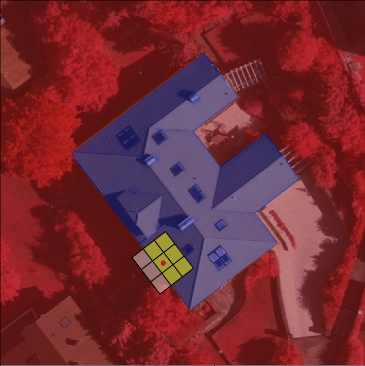
(a)

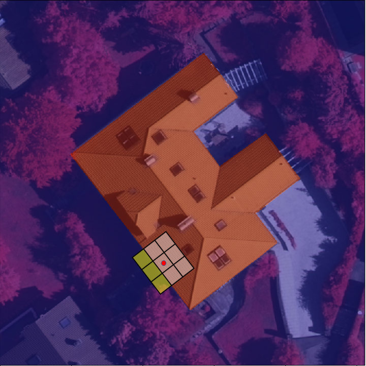
(b)

Figure 2: The filter is divided by the contour into interior and exterior regions. The point $x$ is represented by the red dot and the interior (a) and exterior (b) regions are shaded in yellow.

We compute these local statistics using a characteristic function $W_{s}$ with local window (Figure 2) of size $f_{s}$, as follows:

$$W_{s}=\begin{cases}1&\quad\text{if }x-f_{s}\leq u\leq x+f_{s},\quad y-f_{s}\leq v\leq y+f_{s};\\ 0&\quad\text{otherwise},\\ \end{cases}$$ (6)

where $x,y$ and $u,v$ are the coordinates of two independent points.

We introduce feature maps $\lambda_{1}(x,y)$ and $\lambda_{2}(x,y)$ for learning the foreground and background energies and allow them to be functions over the image domain $\Omega$. Therefore, our energy functional may be written as

$$E(\phi)=\int_{\Omega}\delta(\phi(x,y))\biggl{[}\mu|\nabla\phi(x,y)|+\int_{\Omega}W_{s}F(\phi(u,v))\,du\,dv\biggr{]}\,dx\,dy,$$ (7)

in which $F(\phi)$ is

$$\begin{split}F(\phi)=&\lambda_{1}(x,y)(I(u,v)-m_{1}(x,y))^{2}(H(\phi(x,y))+\\ &\lambda_{2}(x,y)(I(u,v)-m_{2}(x,y))^{2}(1-H(\phi(x,y)).\end{split}$$ (8)

It is important to note that our localized formulation enables us to capture the fine-grained details of boundaries, and our use of pixel-wise masks $\lambda_{1}(x,y)$ and $\lambda_{2}(x,y)$ allows them to be directly predicted by the backbone CNN along with an initialization map $\phi_{0}(x,y)$. Thus, not only does the implicit ACM propagation now become fully automated, but it can also be directly controlled by a CNN through these learnable parameter functions.

2 Euler-Lagrange Partial Differential Equation

Following Lankton and Tannenbaum [73], we now derive the Euler-Lagrange PDE governing the evolution of the ACM.

Using the characteristic function $W_{s}$ that selects regions within a square window of size $s$, the energy functional of contour $C$ in terms of a generic internal energy density $F$ may be written as

$$E(\phi)=\int_{\Omega_{X_{1}}}\delta(\phi(X_{1}))\int_{\Omega_{X_{2}}}W_{s}F(\phi,X_{1},X_{2})\,dX_{2}\,dX_{1},$$ (9)

where $X_{1}=(u,v)$ and $X_{2}=(x,y)$ are two independent spatial variables, each of which represents a point in $\Omega$. To compute the first variation of the energy functional, we add to $\phi$ a perturbation function $\epsilon\psi$, where $\epsilon$ is a small number; hence,

$$E(\phi+\epsilon\psi)=\int_{\Omega_{X_{1}}}\delta(\phi(X_{1})+\epsilon\psi)\int_{\Omega_{X_{2}}}W_{s}F(\phi+\epsilon\psi,X_{1},X_{2})\,dX_{2}\,dX_{1}.$$ (10)

Taking the partial derivative of (10) with respect to $\epsilon$ and evaluating at $\epsilon=0$ yields, according to the product rule,

$$\begin{split}\left.\dfrac{\partial E}{\partial\epsilon}\right|_{\epsilon=0}=\int_{\Omega_{X_{1}}}\delta(\phi(X_{1}))\int_{\Omega_{X_{2}}}\psi W_{s}\nabla_{\phi}F(\phi,X_{1},X_{2})\,dX_{2}\,dX_{1}+\\ \psi\int_{\Omega_{X_{1}}}\gamma\phi(X_{1})\int_{\Omega_{X_{2}}}W_{s}F(\phi,X_{1},X_{2})\,dX_{2}\,dX_{1},\end{split}$$ (11)

where $\gamma\phi$ is the derivative of $\delta(\phi)$. Since $\gamma\phi$ is zero on the zero level set, it does not affect the movement of the curve. Thus the second term in (11) and can be ignored. Exchanging the order of integration, we obtain

$$\left.\dfrac{\partial E}{\partial\epsilon}\right|_{\epsilon=0}=\int_{\Omega_{X_{2}}}\int_{\Omega_{X_{1}}}\psi\delta(\phi(X_{1}))W_{s}\nabla_{\phi}F(\phi,X_{1},X_{2})\,dX_{1}\,dX_{2}.$$ (12)

Invoking the Cauchy–Schwartz inequality yields

$$\frac{\partial\phi}{\partial t}=\int_{\Omega_{X_{2}}}\delta(\phi(X_{1}))W_{s}\nabla_{\phi}F(\phi,X_{1},X_{2})\,dX_{2}.$$ (13)

Adding the contribution of the curvature term and expressing the spatial variables by their coordinates, we obtain the desired curve evolution PDE:

$$\frac{\partial\phi}{\partial t}=\delta(\phi)\biggl{[}\mu\operatorname{div}\left(\frac{\nabla\phi}{|\nabla\phi|}\right)+\int_{\Omega}W_{s}\nabla_{\phi}F(\phi)\,dx\,dy\biggr{]},$$ (14)

where, assuming a uniform internal energy model and defining $m_{1}$ and $m_{2}$ as the mean image intensities inside and outside $C$ and within $W_{s}$, we have

$$\nabla_{\phi}F=\delta(\phi)\left(\lambda_{1}(u,v)[I(u,v)-m_{1}(x,y)]^{2}-\lambda_{2}(u,v)[I(u,v)-m_{2}(x,y)]^{2}\right).$$ (15)

3 DALS CNN Backbone

Our encoder-decoder is an FCN architecture that is tailored and trained to estimate a probability map from which the initial distance function $\phi(x,y,0)$ of the level-set ACM and the functions $\lambda_{1}(x,y)$ and $\lambda_{2}(x,y)$ are computed. In each dense block of the encoder, a composite function of batch normalization, convolution, and ReLU is applied to the concatenation of all the feature maps $[x_{0},x_{1},\dots,x_{l-1}]$ from layers 0 to $l-1$ with the feature maps produced by the current block. This concatenated result is passed through a transition layer before being fed to successive dense blocks. The last dense block in the encoder is fed into a custom multiscale dilation block with 4 parallel convolutional layers with dilation rates of 2, 4, 8, and 16. Before being passed to the decoder, the output of the dilated convolutions are then concatenated to create a multiscale representation of the input image thanks to the enlarged receptive field of its dilated convolutions. This, along with dense connectivity, assists in capturing local and global context for highly accurate lesion localization.

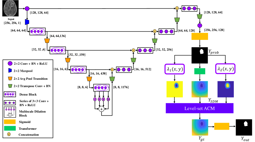
Figure 3: The DALS architecture. DALS is a fully automatic segmentation framework. The CNN initializes and guides the ACM by its learning local weighted parameters.

4 The DALS Framework

Our DALS framework is illustrated in Figure 3. The boundaries of the segmentation map generated by the encoder-decoder are fine-tuned by the level-set ACM that takes advantage of information in the CNN maps to set the per-pixel parameters and initialize the contour. The input image is fed into the encoder-decoder, which localizes the lesion and, after $1\times 1$ convolutional and sigmoid layers, produces the initial segmentation probability map $Y_{\text{prob}}(x,y)$, which specifies the probability that any point $(x,y)$ lies in the interior of the lesion. The Transformer converts $Y_{\text{prob}}$ to a Signed Distance Map (SDM) $\phi(x,y,0)$ that initializes the level-set ACM. Map $Y_{\text{prob}}$ is also utilized to estimate the parameter functions $\lambda_{1}(x,y)$ and $\lambda_{2}(x,y)$ in the energy functional (7). Extending the approach of Hoogi et al. [54], the $\lambda$ functions in Figure 3 are chosen as follows:

$$\lambda_{1}(x,y)=\exp\left(\frac{2-Y_{\text{prob}}(x,y)}{1+Y_{\text{prob}}(x,y)}\right);\quad\lambda_{2}(x,y)=\exp\left(\frac{1+Y_{\text{prob}}(x,y)}{2-Y_{\text{prob}}(x,y)}\right).$$ (16)

The exponential amplifies the range of values that the functions can take. These computations are performed for each point on the zero level set contour $C$. During training, $Y_{\text{prob}}$ and the ground truth map $Y_{\text{gt}}(x,y)$ are fed into a Dice loss function and the error is back-propagated accordingly. During inference, a forward pass through the encoder-decoder and level-set ACM results in a final SDM, which is converted back into a probability map by a sigmoid layer, thus producing the final segmentation map $Y_{\text{out}}(x,y)$.

2 The DTAC Framework

We further propose a model, dubbed Deep Trainable Active Contours (DTAC), that establishes a tight merger between our ACM with any backbone CNN for segmenting images in a robust manner and capture the fine-grained details of their boundaries.

1 Differentiable Level Set

We dynamically evolve the contour according to (14) in a differentiable manner using TensorFlow. The first term, $\operatorname{div}\bigl{(}\frac{\nabla\phi}{|\nabla\phi|}\bigr{)}$, necessitates computing the surface curvature according to

$$\operatorname{div}\left(\frac{\nabla\phi}{|\nabla\phi|}\right)=\dfrac{\phi_{xx}\phi_{y}^{2}-2\phi_{xy}\phi_{x}\phi_{y}+\phi_{yy}\phi_{x}^{2}}{(\phi_{x}^{2}+\phi_{y}^{2})^{3/2}},$$ (17)

where the subscripts denote spatial derivatives of $\phi$, which we compute using central finite differences. For the second term, we find the regions in the image that correspond to the interior and exterior of the curve and leverage average pooling layers to efficiently compute $m_{1}$ and $m_{2}$ used in (8). Therefore we can evaluate $\frac{\partial\phi}{\partial t}$ in (14) and update the level-set according to

$$\phi^{t}=\phi^{t-1}+\Delta t\frac{\partial\phi^{t-1}}{\partial t},$$ (18)

where $\Delta t$ is the time step size.

2 DTAC CNN Backbone

We use a standard encoder-decoder architecture with residual blocks and skip connections between the encoder and decoder sub-networks. Each residual block consists of two convolutions with batch normalization, ReLU, and an additive identity skip connection. As is illustrated in Figure 4, each stage of the encoder comprises of residual blocks and convolutions with stride of two. Similarly, each stage of the decoder has a residual block followed by a transposed convolution. The encoder is connected to the decoder via a residual block at the lowest resolution as well as skip connections at every stage. The output of the decoder is connected to a convolution with three output channels for predicting the $\lambda_{1}(x,y)$ and $\lambda_{2}(x,y)$ feature maps as well as the initialization map $\phi_{0}(x,y)$. Detailed information regarding the encoder and decoder of DTAC is presented in Tables 1 and 2.

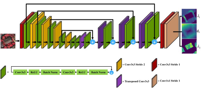
Figure 4: DTAC’s CNN backbone has a standard encoder-decoder architecture.

Operations	Output size
Input	$512\times 512\times 1$
Conv, ReLu, BN	$512\times 512\times 64$
Conv, ReLU, BN, Conv, ReLU, BN, Add	$512\times 512\times 64$
Conv stride 2	$256\times 256\times 128$
Conv, ReLU, BN, Conv, ReLU, BN, Add	$256\times 256\times 128$
Conv stride 2	$128\times 128\times 256$
Conv, ReLU, BN, Conv, ReLU, BN, Add	$128\times 128\times 256$
Conv stride 2	$64\times 64\times 512$
Conv, ReLU, BN, Conv, ReLU, BN, Add	$64\times 64\times 512$
Conv stride 2	$32\times 32\times 1024$
Conv, ReLU, BN, Conv, ReLU, BN, Add	$32\times 32\times 1024$
Conv, ReLU, BN, Conv, ReLU, BN, Add	$32\times 32\times 1024$

Table 1: Detailed information about the encoder of DTAC. BN and Add denote batch normalization and additive identity skip connections. Conv denotes a $3\times 3$ convolutional layer.

Operations	Output size
Input	$32\times 32\times 1024$
TransConv stride 2	$64\times 64\times 512$
Conv, ReLU, BN, Conv, ReLU, BN, Add	$64\times 64\times 512$
TransConv stride 2	$128\times 128\times 256$
Conv, ReLU, BN, Conv, ReLU, BN, Add	$128\times 128\times 256$
TransConv stride 2	$256\times 256\times 128$
Conv, ReLU, BN, Conv, ReLU, BN, Add	$256\times 256\times 128$
TransConv stride 2	$512\times 512\times 64$
Conv, ReLU, BN, Conv, ReLU, BN, Add	$512\times 512\times 64$
Conv, ReLu, BN	$512\times 512\times 32$
Conv1, Sigmoid	$512\times 512\times 3$

Table 2: Detailed information about the decoder of DTAC. BN and Add denote batch normalization and additive identity skip connections. Conv and Conv1 denote $3\times 3$ and $1\times 1$ convolutional layers, respectively. TransConv denotes a $3\times 3$ transposed convolutional layer with a kernel size of 2.

3 The DTAC Architecture and Network Training

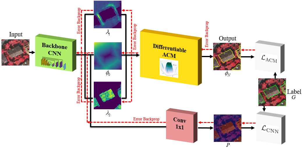
Figure 5: DTAC is a fully-automated, end-to-end automatically differentiable and backpropagation trainable ACM and backbone CNN framework.

We simultaneously train the CNN and levelset components of DTAC in an end-to-end manner with no human supervision. The CNN guides the ACM by predicting the $\lambda_{1}(x,y)$ and $\lambda_{2}(x,y)$ feature maps as well as an initialization map $\phi_{0}(x,y)$. The level set evolves in a differentiable manner, thus allowing for directly backpropagating the error. The initialization map output of the CNN is further passed into another convolution layer followed by a sigmoid activation function (Figure 5). Therefore, the total loss for training the DTAC is

$$\mathcal{L}=\mathcal{L}_{\text{CNN}}+\mathcal{L}_{\text{ACM}},$$ (19)

where $\mathcal{L}_{\text{CNN}}$ and $\mathcal{L}_{\text{ACM}}$ denote the losses computed over the output of backbone CNN and final iteration of level-set ACM, respectively. $\mathcal{L}_{\text{ACM}}$ is computed using a binary cross entropy loss function according to

$$\mathcal{L}_{\text{ACM}}=-\frac{1}{N}\sum_{j=1}^{N}\left[G_{j}\log H(\phi_{j})+(1-G_{j})\log(1-H(\phi_{j}))\right],$$ (20)

where $H$ is defined according to (1), $\phi_{j}$ and $G_{j}$ denote the ACM output and ground truth at pixel $j$ respectively, and $N$ is the total number of pixels in the image. $\mathcal{L}_{\text{CNN}}$ is calculated in a similar manner to (20) by replacing $H_{j}$ with the output prediction probabilities of $P_{j}$ from the CNN. Algorithm 1 presents the details of DTAC training.

Data: $X$, $G$: Paired image and label; $W$: CNN with parameters $\omega$; $g$: ACM energy function with parameters $\lambda_{1},\lambda_{2}$; $\mathcal{L}$: Loss function; $N$: Number of ACM iterations; $\eta$: Learning rate; $\phi$: Levelset; $P$: CNN probability output

Result: Trained model

1 while not converged do

2       $\lambda_{1},\lambda_{2},\phi_{0},P=W(X)$

3       for $t=1$ to $N$ do

4             $\frac{\partial\phi_{t-1}}{\partial t}=g(\phi_{t-1};\lambda_{1},\lambda_{2},X)$

5             $\phi^{t}=\phi^{t-1}+\Delta t\frac{\partial\phi^{t-1}}{\partial t}$

6       end for

7      $\mathcal{L}=\mathcal{L}_{\text{ACM}}(\phi_{N},G)+\mathcal{L}_{\text{CNN}}(P,G)$

8       Compute $\frac{\partial\mathcal{L}}{\partial\omega}$ and backpropagate the error

9       Update the weights of $f$: $\omega\leftarrow\omega-\eta\frac{\partial\mathcal{L}}{\partial\omega}$

10 end while

Algorithm 1 DTAC Training Algorithm

Chapter 4 Few-Shot Semantic Segmentation

In this chapter, we propose a novel metric-based framework for few-shot image segmentation, which we call Segmentation with Aligned Variational Auto-Encoders (SegAVA), that explores the latent and image spaces of support and query sets to find the most common class-specific embeddings and fuses them to produce the final semantic segmentation (Figure 1). Specifically, SegAVA features a latent stream consisting of two Variational Auto-Encoders (VAEs) that generate support and query images and learn the most essential discriminative information by aligning their learned features in the latent space.

Figure 1: Overview of the SegAVA architecture, showing the two parallel branches. In the image space branch, SegAVA maps the support and query images to embedding features, learning features for each class (represented by the red, green, and yellow circles), matching query features to the nearest embedded feature. In the latent space branch, SegAVA employs two variational auto-encoders to learn the latent space of support and query images and uses Wasserstein-2 metric to learn similarities between embeddings. Results from the two branches are concatenated and passed through convolutional layers, yielding the final segmentation of the query image.

Additionally, SegAVA uses an encoder-decoder in the image space to extract the most similar features of the support and query images and concatenate them with the learned embeddings of the latent space to produce the segmentation in an end-to-end manner without additional post-processing.

We argue that the latent space of the support and query sets provides rich semantics for identifying the most essential discriminative features, and aggregation with image space embeddings leads to improved segmentation accuracy. Our work can be regarded an extension to that of Deudon [28] who used the latent space for learning semantic similarity in natural language processing, but differs in that SegAVA is trained jointly for image generation and semantic similarity extraction.

1 Problem Setting

In the $N$-way $k$-shot semantic segmentation problem, given a training set of $K$ samples with $N$ classes, the goal is to learn to segment new images with categories that belong to the $N$ classes. We follow the same training and testing protocols in prior efforts [101; 122] and formulate our problem as follows: Given, two sets of non-overlapping seen and unseen categories, denoted as $\mathcal{C}_{\text{unseen}}$ and $\mathcal{C}_{\text{seen}}$, we define two sets for training and testing the model. The train set $\mathcal{D}_{\text{train}}$ = {${(\mathcal{S}_{i},\mathcal{Q}_{i})}_{i=1}^{N_{\text{train}}}$} and test set $\mathcal{D}_{\text{test}}$ = {${(\mathcal{S}_{i},\mathcal{Q}_{i})}_{i=1}^{N_{\text{test}}}$} are defined in a sequence of episodes. Each episode, denoted by $i$, has a set of support samples $\mathcal{S}_{i}$ and query samples $\mathcal{Q}_{i}$ with total numbers $N_{\text{train}}$ and $N_{\text{test}}$ for the train and test episodes, respectively.

In a $N$-way, $k$-shot setting, the episode $i$ comprises a support set $\mathcal{S}_{i}$ = {($\mathcal{I}_{c,k}$, $\mathcal{L}_{c,k}$)} in which for each class, there exist $K$ samples of image and label pairs, and there are $N$ distinct semantic classes in total. Furthermore, from the categories that are present in the support set, there are $N_{\text{query}}$ samples of image and label pairs in the the query set. In each training episode, the goal is to utilize the support set $\mathcal{S}_{i}$, with images $\mathcal{I}$ and corresponding pixel-wise annotations $\mathcal{L}$, to segment images in the query set $\mathcal{Q}_{i}$. Eventually, the trained segmentation model is employed to perform segmentation on the cases from the test set $\mathcal{D}_{\text{test}}$ in each of its episodes.

2 SegAVA Framework

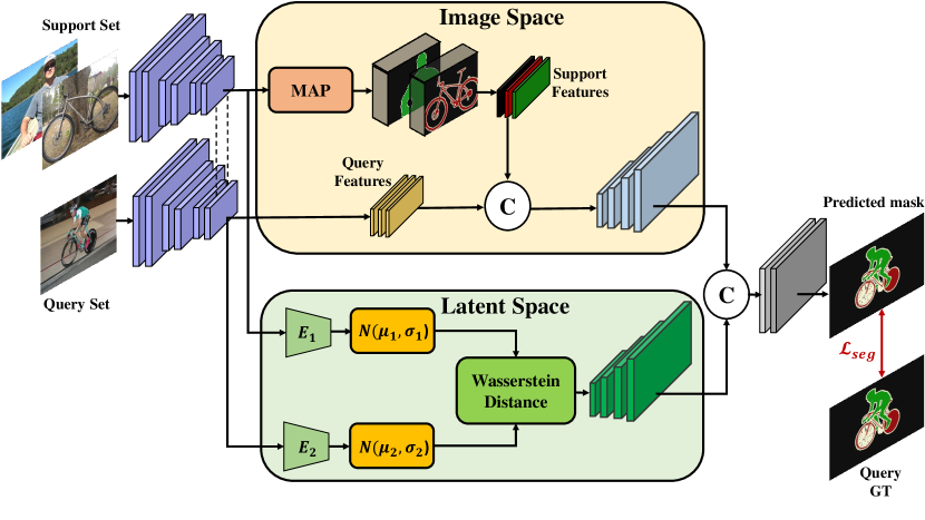
Figure 2: Detailed diagram of the SegAVA architecture. MAP denotes the Masked Average Pooling operation. $E_{1}$ and $E_{2}$ denote the encoders of support and query features, respectively. The pretrained feature extractor of support and query sets share the same weights.

As illustrated in Figure 2, images in the support and query sets are first fed into a pre-trained network for initial feature extraction, and the extracted features are subsequently aligned in the image space (upper stream) as well as the latent space (lower stream). The aligned features in both latent and image space are further concatenated and fed into a series of convolutional layers that produce the final segmentation. We detail the working principles of feature alignments in the next two sections.

3 Latent Space Alignment

In SegAVA, the building blocks of feature alignment in the latent space are VAEs [70]. Given a VAE with an encoder $\phi$, decoder $\theta$, and input $x$, the goal of the encoder is to parameterize $p_{\theta}(z\mid x)$ over the latent variable $z$. Furthermore, the decoder parameterizes $p_{\theta}(z\mid x)$ over $x$, given a random latent variable $z$. Using a variational lower bound limit on the marginal likelihood of $p(x\mid\theta,\phi)$, the VAE loss function can be expressed as

$$\mathcal{L}=\mathbbm{E}_{q_{\phi}(z\mid x)}[\text{log}p_{\theta}(x\mid z)]-\text{KL}(q_{\phi}(z\mid x)\,||\,p(z)),$$ (1)

where the first term represents the reconstruction error and the second term is the Kullback-Leibler (KL) divergence between the prior on the latent code $p(z)$ and a posterior distribution $q_{\phi}(z\mid x)$. The decoder predicts the posterior, normally a Gaussian distribution such that $q_{\phi}(z\mid x)=\mathcal{N}(\mu,\sigma).$ Consequently, the final loss function of SegAVA’s VAEs, for the support and query sets is

$$\mathcal{L}_{\text{VAE}}=\sum_{i}^{M=2}\mathbbm{E}_{q_{\phi}(z\mid x)}[\log p_{\theta}(x^{(i)}\mid z)]-\text{KL}[q_{\theta}(z\mid x^{(i)})\,||\,p_{\theta}(z)].$$ (2)

Inspired by [28], we further utilize a Wasserstein-2 metric between the latent multivariate Gaussian distributions of the support and query sets for alignment in the latent space, according to

$$W_{2}^{2}(p_{1},p_{2})=\sum_{i}(\mu_{1}^{i}-\mu_{2}^{i})^{2}+(\sigma_{1}^{i}-\sigma_{2}^{i})^{2},$$ (3)

where $p_{1}=\mathcal{N}(\mu_{1},\sigma_{1})$ and $p_{2}=\mathcal{N}(\mu_{2},\sigma_{2})$, the diagonal covariance matrices of two Gaussians. It is important to note that we utilize (3) in an element-wise manner and feed the result it to a dense layer followed by a fully convolutional decoder to estimate the similarity between the support and query embeddings.

4 Image Space Alignment

In the image space, query and support images are first fed into a pre-trained network to obtain feature embeddings that can be used to estimate the similarities. Given a support set $\mathcal{S}_{i}$ = {($\mathcal{I}_{c,k}$, $\mathcal{L}_{c,k}$)} in which $c$ denotes the index corresponding to each semantic class and $k=1,2,\ldots,K$ is the index for each sample in the support set, we use a masked average pooling operation [135],

$$p_{c}=\frac{1}{K}\sum_{k}\frac{\sum_{x,y}F_{c,k}^{(x,y)}\mathbbm{1}[\mathcal{L}_{c,k}^{(x,y)}=c]}{\sum_{x,y}\mathbbm{1}[\mathcal{L}_{c,k}^{(x,y)}=c]},$$ (4)

where $(x,y)$ are spatial location indexes and $F_{c,k}^{(x,y)}$ are the extracted features for an input image $\mathcal{I}_{c,k}$ at spatial location $(x,y)$. Subsequently, the masked features are fed into a fully convolutional decoder each layer of which consists of a $3\times 3$ transposed convolution with stride of $2$ followed by a batch normalization [60] operation and a ReLU activation function.

Furthermore, the upsampled similarity features from the image space are concatenated with decoded features from the latent space and fed into a $3\times 3$ convolution followed by a $1\times 1$ convolution. The output segmentation map is subsequently calculated according to

$$\tilde{L}_{q;j}^{(x,y)}=\frac{\exp(F_{q}^{(x,y)})}{\sum_{p_{j}\in\mathcal{P}}\exp(F_{q}^{(x,y)})},$$ (5)

where $F_{q}^{(x,y)}$ is the pixel-wise output of the last convolutional layer. Accordingly, the segmentation loss can be defined as

$$\mathcal{L}_{\text{seg}}=-\frac{1}{N}\sum_{x,y}\sum_{p_{j}\in\mathcal{P}}\mathbbm{1}[L_{q}^{(x,y)}=j]\log\tilde{L}_{q;j}^{(x,y)},$$ (6)

where $L_{q}^{(x,y)}$ and $\tilde{L}_{q;j}^{(x,y)}$ denote the ground-truth and predictions at spatial location $(x,y)$. To jointly train the latent and image streams, we use the hybrid loss function

$$\mathcal{L}_{\text{SegAVA}}=\mathcal{L}_{\text{seg}}+\gamma\mathcal{L}_{\text{VAE}},$$ (7)

where $\gamma$ is a hyper-parameter.

5 Active Contour Assisted Few-Shot Segmentation

SegAVA can additionally benefit from a post-processing module that can refine the segmentation predictions. As such, we leveraged our DALS framework to fully delineate the boundaries.

The probability predictions by SegAVA are used to initialize the contour as well as the $\lambda_{1}(x,y)$ and $\lambda_{2}(x,y)$ feature maps. The contour $C$ is then evolved according to

$$\frac{\partial\phi}{\partial t}=\delta(\phi)\biggl{[}\mu\operatorname{div}\left(\frac{\nabla\phi}{|\nabla\phi|}\right)+\int_{\Omega}W_{s}\nabla_{\phi}F(\phi)\,dx\,dy\biggr{]},$$ (8)

where $m_{1}$ and $m_{2}$ denote the mean image intensities inside and outside $C$, and

$$\nabla_{\phi}F=\delta(\phi)\bigl{(}\lambda_{1}(u,v)(I(u,v)-m_{1}(x,y))^{2}-\lambda_{2}(u,v)(I(u,v)-m_{2}(x,y))^{2}\bigr{)}.$$ (9)

Chapter 5 Implementation Details, Data, Experiments, Results

This chapter presents our experiments with the models that we developed in Chapters 2, 3, and 4, and it reports our results. We also provide information about the datasets that we use in our empirical studies and implementation details about the models themselves.

1 2D Edge-Aware Encoder-Decoders

In this section, we empirically study the models developed in Section 1.

1 Dataset

In our experiments, we used the BraTS 2018 [8], which provides multimodal 3D brain MRIs and ground truth brain tumor segmentations annotated by physicians, consisting of 4 MRI modalities per case (T1, T1c, T2, and FLAIR). Annotations include 3 tumor subregions—the enhancing tumor, the peritumoral edema, and the necrotic and non-enhancing tumor core. The annotations were combined into 3 nested subregions—whole tumor (WT), tumor core (TC), and enhancing tumor (ET). The data were collected from 19 institutions, using various MRI scanners.

For simplicity, we use only a single input MRI modality (T1c) and aim to segment a single tumor region—TC, which includes the main tumor components (nectrotic core, enhancing, and non-enhancing tumor regions). Furthermore, even though the original data is 3D ($240\times 240\times 155$), we operate on 2D slices for simplicity. We have extracted several axial slices centered around the tumor region from each 3D volume, and combined them into a new 2D dataset.

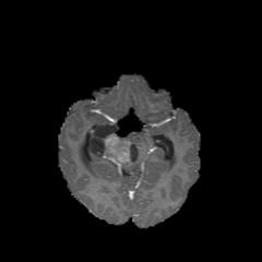
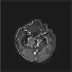
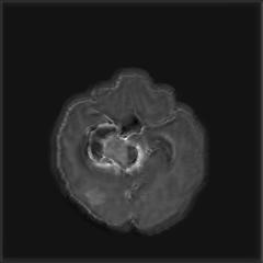
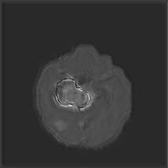
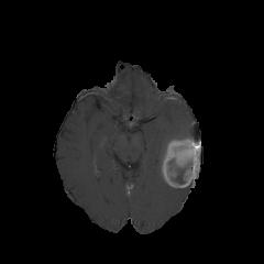
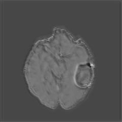
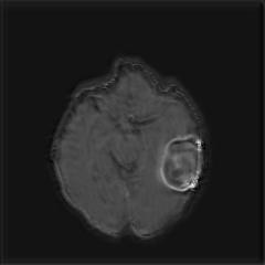
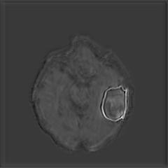
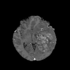
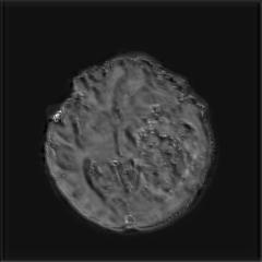
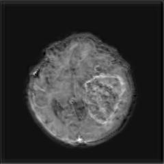
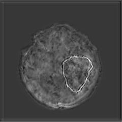
(a) Input image (b) Att. Layer 1 (c) Att. Layer 2 (d) Att. Layer 3

Figure 1: Visualization of learned feature maps in 2D edge-aware network. (b–d) Outputs of the attention layers. The boundary emphasis becomes more prominent with each attention layer.

2 Implementation Details

We have implemented our model in Tensorflow. The brain input images were resized to predefined sizes of $240\times 240$ and normalized to the intensity range $[0,1]$. The model was trained on NVIDIA Titan RTX and an Intel® Core™ i7-7800X CPU @ 3.50GHz $\times$ 12 with a batch size of 8 for all models. We used $\lambda_{1}=1.0$, $\lambda_{2}=0.5$, and $\lambda_{3}=0.1$ in (3). The Adam optimization algorithm was used with initial learning rate of $\alpha_{0}=1.0^{-3}$ and further decreased according to

$$\alpha=\alpha_{0}\left(1-e/N_{e}\right)^{0.9},$$ (1)

where $e$ denotes the current epoch and $N_{e}$ the total number of epochs, following [92]. We have evaluated the performance of our model by using the Dice score, Jaccard index, and Hausdorff distance.

3 Results

Boundary Stream:

Figure 1 demonstrates the output of each of the attention layers in our dedicated boundary stream. In essence, each attention layer progressively localizes the tumor and refines the boundaries. The first attention layer has learned rough estimate of the boundaries around the tumor and localized it, whereas the second and third layers have learned more fine-grained details of the edges and boundaries, refining the localization.

Moreover, since our architecture leverages a dilated spatial pyramid pooling to merge the learned feature maps of the regular segmentation stream and the boundary stream, multiscale regional and boundary information have been preserved and fused properly, which has enabled our network to capture the small structural details of the tumor.

Model	Dice Score	Jaccard Index	Hausdorff Distance
U-Net	0.731$\pm$0.230	0.805 $\pm$0.130	3.861$\pm$1.342
V-Net	0.769$\pm$0.270	0.837$\pm$0.140	3.667$\pm$1.329
Ours (no edge loss)	0.768$\pm$0.236	0.832$\pm$0.136	3.443$\pm$1.218
Ours	0.822$\pm$0.176	0.861$\pm$0.112	3.406$\pm$1.196

Table 1: Performance evaluations of different models. We validate the contribution of the edge loss by measuring performance with and without this layer.

Edge-Aware Losses:

To validate the effectiveness of the loss supervision, we have trained our network without enforcing the supervision of the edge loss during the learning process, but with the same architecture. Table 1 shows that our network performs very similarly to V-Net [87] without edge supervision, since ours employs similar residual blocks as V-Net in its main encoder-decoder. In essence, the boundary stream also impacts the downstream layers of the encoder by emphasizing edges during training.

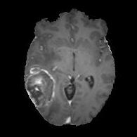
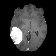
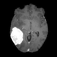
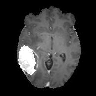
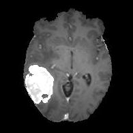
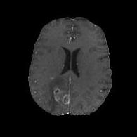
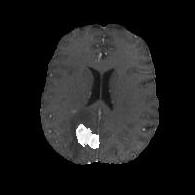
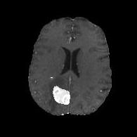
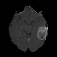
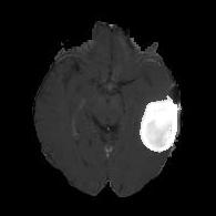
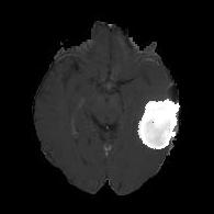
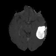
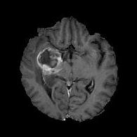
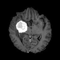
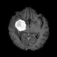
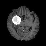
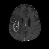
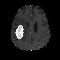
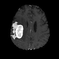
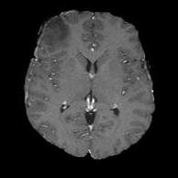
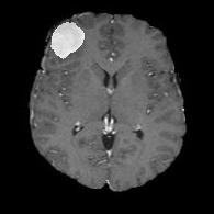
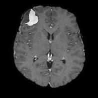
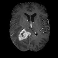
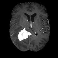
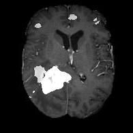
(a) Input image (b) Label (c) Ours (d) V-Net (e) U-Net

Figure 2: Qualitative comparison of 2D edge-aware predictions.

Comparison to Competing Methods:

We have compared the performance of our model against the most popular deep learning-based semantic segmentation networks, U-Net [102] and V-Net [87] (Figure 2). Our model outperforms both by a considerable margin in all evaluation metrics. In particular, U-Net performs poorly in most cases due to the high false positive of its segmentation predictions, as well as the imprecision of its boundaries. The powerful residual block in the V-Net architecture seems to alleviate these issues to some extent, but V-Net also fails to produce high-quality boundary predictions. The emphasis of learning useful edge-related information during the training of our network appears to effectively regularize the network such that boundary accuracy is improved.

2 3D Edge-Aware Encoder-Decoders

In this section, we empirically study the models developed in Section 2.

1 Dataset

Kidney Tumor Segmentation Challenge (KiTS 2019) provides data of multi-phase 3D CTs, voxel-wise ground truth labels, and comprehensive clinical outcomes for 300 patients who underwent nephrectomy for kidney tumors between 2010 to 2018 at University of Minnesota [53]. 210 patients were randomly selected for the training set and the remaining 90 patients were left as a testing set. The annotation was performed in the transverse plane with regular subsampling of series in the longitudinal direction with roughly 50 annotated slices depicting the Kidney for each patient. The labels for excluded slices were computed by using a contour interpolation algorithm [53].

2 Evaluation metrics

We have adopted the same three evaluation metrics as outlined by KiTS 2019 challenge. Kidneys dice denote the segmentation performance when considering both kidneys and tumors as the foreground whereas tumor dice considers everything except the tumor as background. Composite dice is simply the average of kidneys dice and tumor dice.

3 Results

Table 2 represents the evaluation results of our model on our own dataset partition. We divided the training set of KiTS 2019 dataset into our own subsets for training and validation and evaluated the performance of a our proposed model. Figure 3 illustrates the segmentation visualizations of our method and their corresponding ground truth from two cases in the validation set of our own partition.

Kidneys Dice	Tumor Dice	Composite Dice
0.96	0.82	0.89

Table 2: Evaluation results of the 3D edge-aware network on the KiTS 2019 test set.

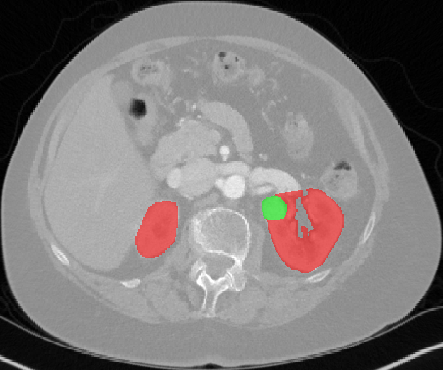
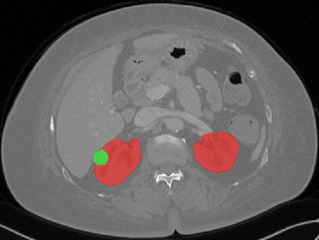
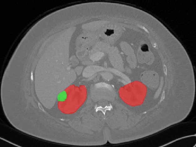
(a) Our Predictions (b) Ground truth Labels

Figure 3: Visualization of (a) our model’s predictions and (b) ground truth labels.

3 Plug-and-Play Edge-Aware CNNs

In this section, we empirically study the models developed in Section 3.

1 Implementation Details

DALS is implemented in Tensorflow [1]. We trained it on an NVIDIA Titan XP GPU and an Intel® Core™ i7-7700K CPU @ 4.20GHz. All the input images were first normalized and resized to a predefined size of $256\times 256$ pixels. The size of the mini-batches is set to 4, and the Adam optimization algorithm was used with an initial learning rate of 0.001 that decays by a factor of 10 every 10 epochs. The entire inference time for DALS takes $1.5$ seconds. All model performances were evaluated by using the Dice coefficient, Hausdorff distance, and BoundF.

Model	Edge	Average Dice	ET Dice	TC Dice	WT Dice
U-Net	None	0.8305$\pm$0.0035	0.7375$\pm$0.0021	0.8480$\pm$0.0056	0.9060$\pm$0.0021
V-Net	None	0.8281$\pm$0.0035	0.7255$\pm$0.0049	0.8570$\pm$0.0042	0.9020$\pm$0.0014
Seg-Net	None	0.8300$\pm$0.0033	0.7330$\pm$0.0042	0.8550$\pm$0.0049	0.9015$\pm$0.0007
U-Net	EG-CNN	0.8406$\pm$0.0028	0.7530$\pm$0.0113	0.8630$\pm$0.0014	0.9006$\pm$0.0042
V-Net	EG-CNN	0.8386$\pm$0.0051	0.7460$\pm$0.0056	0.8605$\pm$0.0035	0.9095$\pm$0.0063
Seg-Net	EG-CNN	0.8570$\pm$0.0007	0.7680$\pm$0.0113	0.8850$\pm$0.0070	0.9180$\pm$0.0028

Table 3: Evaluation results on the BraTS 2019 dataset in terms of overall and tumor subregions Dice scores. The Edge column determines whether EG-CNN is utilized with the backbone architecture.

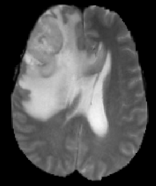
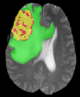
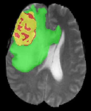
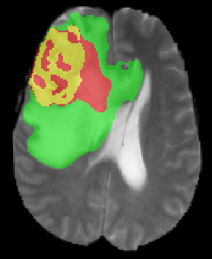
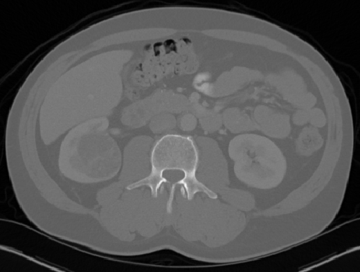
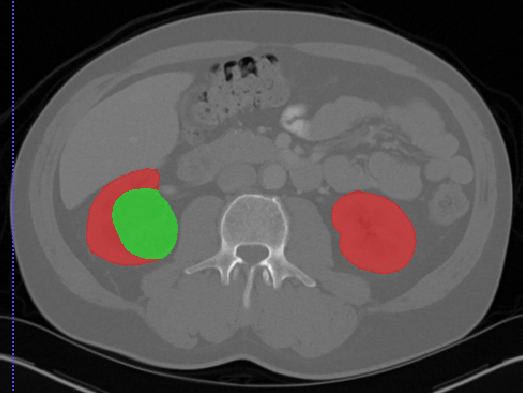
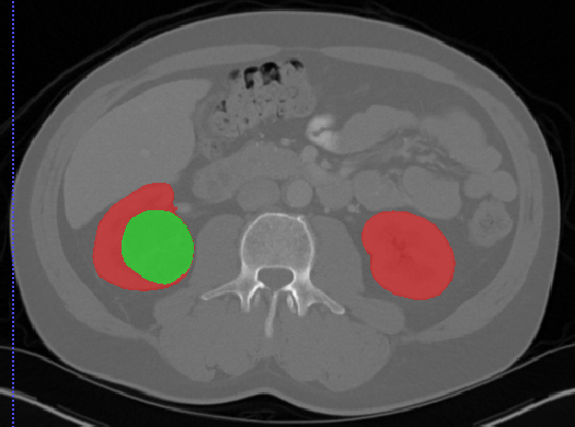
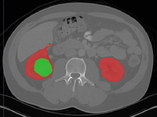
(a) Input images (b) Semantic Labels (c) Seg-Net+EG-CNN (d) Seg-Net

Figure 4: Visualization of the in-plane segmentation outputs for tumor subregions in the BraTS 2019 dataset. Red, green, and yellow labels denote TC, WT, and ET subregions, respectively.

2 Results

We evaluated the EG-CNN module when it is used to augment popular medical image segmentation models: U-Net [102], V-Net [87], and Seg-Net [90]. We modified each architecture to adopt them to the given task and to be similar to the others for a more fair comparison. For both the U-net and V-net, we changed the normalization to Groupnorm, to better handle a small batch size, and adjusted the number of layers to a roughly equivalent number between the networks. For each dataset we trained the main CNN segmentation network with and without the EG-CNN in order to validate the contribution of our proposed module. We estimated the accuracy of each model in terms of Dice score for each class and of the overall average.

BraTS 2019

Table 3 reports the accuracy of the model on each of the classes: Whole Tumor (WT), Tumor Core (TC), and Enhancing Tumor (ET), as well as the overall overage accuracy. According to our benchmarks, including the EG-CNN consistently increases the overall and subregion Dice scores in all cases. In the case of brain tumor segmentation, the EG-CNN has effectively learned highly complex and irregular boundaries of certain subregions. Therefore, it improves the segmentation quality around the edges, which leads to overall better segmentation performance. Figure 4 illustrates how the addition of the EG-CNN to a standalone Seg-Net [90] improves the quality of segmentation.

The quality of the predicted edges also validates the effectiveness of our proposed edge-aware loss function, since the boundaries are crisp and avoid the thickening effect around edges. Such a phenomenon usually occurs when a naive loss function such as binary cross entropy is utilized for the task of edge prediction without taking precautions. Moreover, our model results in more fine-grained boundaries and visually attractive edges because the learned predicted boundaries are eventually fused with the final prediction output of the main encoder-decoder architecture.

Since the addition of the EG-CNN module increases the number of free parameters of the overall model, we have also experimented with larger standalone models (by increasing their depth and/or width), but doing so did not result in the better validation accuracy. This indicates that our module improves the overall segmentation accuracy not due to the model capacity increase, but due to the extra emphasis of edge information.

Model	Edge	Kidneys Dice	Tumor Dice	Composite Dice
U-Net	None	0.9515$\pm$0.0049	0.8245$\pm$0.0091	0.8880$\pm$0.0070
V-Net	None	0.9370$\pm$0.0065	0.8072$\pm$0.0072	0.8720$\pm$0.0068
Seg-Net	None	0.9530$\pm$0.0028	0.8235$\pm$0.0049	0.8892$\pm$0.0038
U-Net	EG-CNN	0.9620$\pm$0.0056	0.8270$\pm$0.0084	0.8945$\pm$0.0070
V-Net	EG-CNN	0.9483$\pm$0.0048	0.8275$\pm$0.0087	0.8879$\pm$0.0067
Seg-Net	EG-CNN	0.9647$\pm$0.0051	0.8353$\pm$0.0025	0.9000$\pm$0.0038

Table 4: Evaluation results of EG-CNN on the KiTS 2019 dataset for kidneys, tumor, and composite Dice functions. The Edge column determines whether EG-CNN is utilized with the backbone architecture.

(a) Input images (b) Semantic Labels (c) Seg-Net+EG-CNN (d) Seg-Net

Figure 5: Visualization of the segmentation performance of Seg-Net and Seg-Net+EG-CNN on the KiTS 2019 challenge. The green and red masks denote tumor and kidneys, respectively.

KiTS 2019

The achieved accuracy of the model for kidneys and kidney tumor classes, as well as the overall accuracy are presented in Table 4. Similar to the results achieved on the BraTS 2019 dataset, the addition of EG-CNN has consistently improved the segmentation performance. Visual comparisons of the output segmentation and boundary predictions are presented in Figure 5. As such, the predicted edges visually conform to the region outlines, demonstrating that the EG-CNN module and our proposed loss functions helped to captured the details of the edges. This has also been reflected in the final predictions of semantic masks.

4 Deep Active Lesion Segmentation

In this section, we empirically study the models developed in Section 1.

1 Multiorgan Lesion Segmentation (MLS) Dataset

Organ	Modality	# Samples	$\text{Mean}_{\text{GC}}$	$\text{Var}_{\text{GC}}$	$\text{Mean}_{\text{GH}}$	$\text{Var}_{\text{GH}}$	Lesion Radius (pixels)
Brain	MRI	369	0.56	0.029	0.907	0.003	17.42 $\pm$ 9.516
Lung	CT	87	0.315	0.002	0.901	0.004	15.15 $\pm$ 5.777
Liver	CT	112	0.825	0.072	0.838	0.002	20.483 $\pm$ 10.37
Liver	MRI	164	0.448	0.041	0.891	0.003	5.459 $\pm$ 2.027

Table 5: MLS dataset statistics. GC and GH denote Global Contrast and Global Heterogeneity, respectively.

As shown in Table 5, the MLS dataset includes images of highly diverse lesions in terms of size and spatial characteristics such as contrast and homogeneity. The liver component of the dataset consists of 112 contrast-enhanced CT images of liver lesions (43 hemangiomas, 45 cysts, and 24 metastases) with a mean lesion radius of 20.483 $\pm$ 10.37 pixels and 164 liver lesions from 3T gadoxetic acid enhanced MRI scans (one or more LI-RADS (LR), LR-3, or LR-4 lesions) with a mean lesion radius of 5.459 $\pm$ 2.027 pixels. The brain component consists of 369 preoperative and pretherapy perfusion MR images with a mean lesion radius of 17.42 $\pm$ 9.516 pixels. The lung component consists of 87 CT images with a mean lesion radius of 15.15 $\pm$ 5.777 pixels. For each component of the MLS dataset, we used 85% of its images for training, 10% for testing, and 5% for validation.

2 Results

Dataset	Model	Dice	CI	Hausdorff	CI	BoundF
Brain MR	U-Net	0.776 $\pm$ 0.214	0.090	2.988 $\pm$ 1.238	0.521	0.826
	CNN Backbone	0.824 $\pm$ 0.193	0.078	2.755 $\pm$ 1.216	0.490	0.891
	Level-set	0.796 $\pm$ 0.095	0.038	2.927 $\pm$ 0.992	0.400	0.841
	DALS	0.888 $\pm$ 0.0755	0.030	2.322 $\pm$ 0.824	0.332	0.944
Lung CT	U-Net	0.817 $\pm$ 0.098	0.0803	2.289 $\pm$ 0.650	0.530	0.898
	CNN Backbone	0.822 $\pm$ 0.115	0.0944	2.254 $\pm$ 0.762	0.6218	0.900
	Level-set	0.789 $\pm$ 0.078	0.064	3.270 $\pm$ 0.553	0.451	0.879
	DALS	0.869 $\pm$ 0.113	0.092	2.095 $\pm$ 0.623	0.508	0.937
Liver MR	U-Net	0.769 $\pm$ 0.162	0.093	1.645 $\pm$ 0.598	0.343	0.920
	CNN Backbone	0.805 $\pm$ 0.193	0.110	1.347 $\pm$ 0.671	0.385	0.939
	Level-set	0.739 $\pm$ 0.102	0.056	2.227 $\pm$ 0.576	0.317	0.954
	DALS	0.894 $\pm$ 0.065	0.036	1.298 $\pm$ 0.434	0.239	0.987
Liver CT	U-Net	0.698 $\pm$ 0.149	0.133	4.422 $\pm$ 0.969	0.866	0.662
	CNN Backbone	0.801 $\pm$ 0.178	0.159	3.813 $\pm$ 1.791	1.600	0.697
	Level-set	0.765 $\pm$ 0.039	0.034	3.153 $\pm$ 0.825	0.737	0.761
	DALS	0.846 $\pm$ 0.090	0.080	3.113 $\pm$ 0.747	0.667	0.773

Table 6: Quantitative comparison of segmentation performance of DALS and other methods on the MLS dataset. CI denotes the confidence interval.

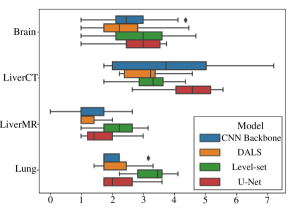
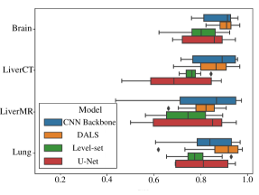
(a) (b)

Figure 6: Box and whisker plots of: (a) Dice score; (b) Hausdorff distance.

Algorithm Comparison

We have quantitatively compared our DALS against U-Net [102] and manually-initialized level-set ACM with scalar $\lambda$ parameter constants as well as its backbone CNN. The evaluation metrics for each organ are reported in Table 6 and box and whisker plots are shown in Figure 6. Our DALS achieves superior accuracies under all metrics and in all datasets. Furthermore, we evaluated the statistical significance of our method by applying a Wilcoxon paired test on the calculated Dice results. Our DALS performed significantly better than the U-Net ($p<0.001$), the manually-initialized ACM ($p<0.001$), and DALS’s backbone CNN on its own ($p<0.005$).

As shown in Figure 8, the DALS segmentation contours conform appropriately to the irregular shapes of the lesion boundaries, since the learned parameter maps, $\lambda_{1}(x,y)$ and $\lambda_{2}(x,y)$, provide the flexibility needed to accommodate the irregularities. In most cases, the DALS has also successfully avoided local minima and converged onto the true lesion boundaries, thus enhancing segmentation accuracy. DALS performs well for different image characteristics, including low contrast lesions, heterogeneous lesions, and noise.

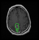
(a) Labeled Img

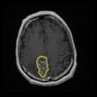
(b) Level Set

(c) DALS

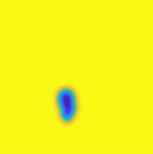
(d) $\lambda_{1}(x,y)$

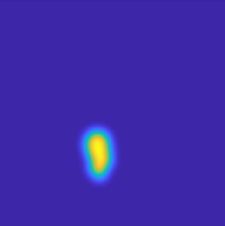
(e) $\lambda_{2}(x,y)$

Figure 7: Visualization of estimated parameter maps. (a) Labeled image. (b) Level-set (analogous to scalar $\lambda$ parameter constants). (c) DALS output. (d), (e) Learned parameter maps $\lambda_{1}(x,y)$ and $\lambda_{2}(x,y)$.

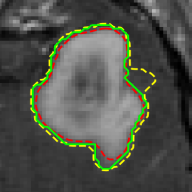
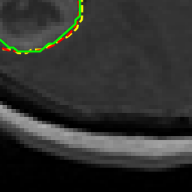
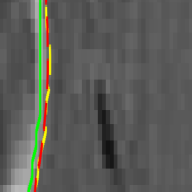
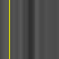
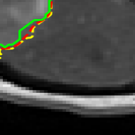
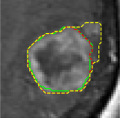
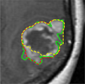
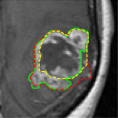
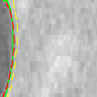
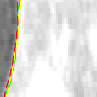
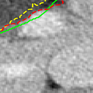
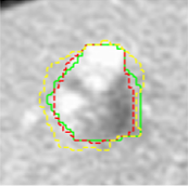
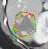
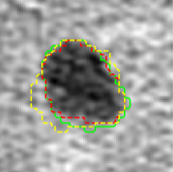
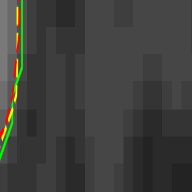
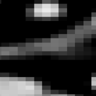
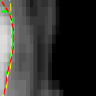
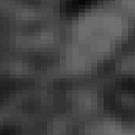
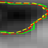
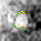
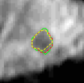
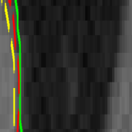
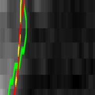
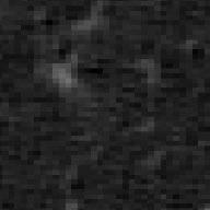
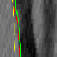
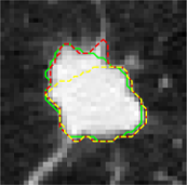
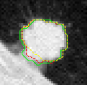
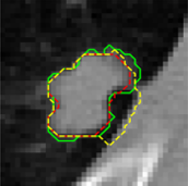
Figure 8: Comparison of the output segmentation of our DALS (red) against the U-Net (yellow) and ground truth (green).

The contribution of the parameter functions was validated by comparing the DALS against a manually initialized level-set ACM with scalar parameters constants as well as with DALS’s backbone CNN on its own. As shown in Figure 7, the encoder-decoder has predicted the $\lambda_{1}(x,y)$ and $\lambda_{2}(x,y)$ feature maps to guide the contour evolution. The learned maps serve as an attention mechanism that provides additional degrees of freedom for the contour to adjust itself precisely to regions of interest.

The segmentation outputs of our DALS and the manual level-set ACM in Figure 7 demonstrate the benefits of using parameter functions to accommodate significant boundary complexities. Moreover, our DALS outperformed the manually-initialized ACM and its backbone CNN in all metrics across all evaluations on every organ.

5 Trainable Deep Active Contours

In this section, we empirically study the models developed in Section 2.

1 Datasets

Vaihingen

The Vaihingen buildings dataset consists of 168 building images of size $512\times 512$ pixels. The labels for each image are generated by using a semi-automated approach. We used 100 images for training and 68 for testing, following the same data partition as in [83]. In this dataset, almost all the images contain multiple instances of buildings, some of which are located at the image edges.

Bing Huts

The Bing Huts dataset consists of 605 images of size $64\times 64$ pixels. We followed the same data partition used in [83], employing 335 images for training and 270 images for testing. This dataset is especially challenging due the low spatial resolution and contrast of the images.

2 Evaluation Metrics

To evaluate our model’s performance, we utilized four different metrics—Dice, mean Intersection over Union (mIoU), Boundary F (BoundF) [25], and Weighted Coverage (WCov) [112].

The Dice (F1) score of an image given the ground truth mask $G$ and the prediction $Y$ is

$$\text{Dice}(G,Y)=\frac{2\sum_{i=1}^{N}G_{i}Y_{i}}{\sum_{i=1}^{N}G_{i}^{2}+\sum_{i=1}^{N}Y_{i}^{2}+\epsilon},$$ (2)

where $G_{i}$ and $Y_{i}$ denote a pixels in $G$ and $Y$, and $N$ is the number of pixels in the image.

Similarly, the IoU score measures the overlap of two objects by calculating the ratio of intersection over union according to

$$\text{IoU}(G,Y)=\frac{|G\cap Y|}{|G\cup Y|}.$$ (3)

BoundF computes the average of Dice scores over 1 to 5 pixels around the boundaries of the groundtruth.

In WConv, the maximum overlap output is selected and the IoU between the ground truth and best output is calculated. IoUs for all instances are summed up and weighted by the area of the ground truth instance. Assuming that $S_{G}=\{r_{1}^{S_{G}},\dots,r_{|S_{G}|}^{S_{G}}\}$ is a set of ground truth regions and $S_{Y}=\{r_{1}^{S_{Y}},\dots,r_{|S_{Y}|}^{S_{Y}}\}$ is a set of prediction regions for single image, and $|r_{j}^{S_{G}}|$ is the number of pixels in $r_{j}^{S_{G}}$, the weighted coverage can be expressed as

$$\text{WCov}(S_{G},S_{Y})=\frac{1}{N}\sum_{j=1}^{|S_{G}|}{|r_{j}^{S_{G}}|}\max\limits_{k=1...|S_{Y}|}\text{IoU}(r_{j}^{S_{G}},r_{k}^{S_{Y}}).$$ (4)

3 Ablation Studies

Single Instance Segmentation

Method		Vaihingen				Bing Huts
Approach	Backbone	Dice	mIoU	WCov	BoundF	Dice	mIoU	WCov	BoundF
FCN	UNet	87.40	78.60	81.80	40.20	77.20	64.90	75.70	41.27
FCN	ResNet	84.20	75.60	77.50	38.30	79.90	68.40	76.14	39.19
FCN	Mask R-CNN	86.00	76.36	81.55	36.80	77.51	65.03	76.02	65.25
FCN	Ours	79.30	66.50	68.60	68.0	80.23	66.98	77.15	40.19
FCN	DSAC	–	81.00	81.40	64.60	–	69.80	73.60	30.30
FCN	DarNet	–	87.20	86.80	76.80	–	74.50	77.50	37.70
DSAC	DSAC	–	71.10	70.70	36.40	–	38.70	44.60	37.10
DSAC	DarNet	–	60.30	61.10	24.30	–	57.20	63.00	15.90
DarNet	DarNet	93.66	88.20	88.10	75.90	85.21	75.20	77.00	38.00
DTAC, Const $\lambda$	Ours	91.18	83.79	82.70	73.21	84.53	73.02	74.21	48.25
DTAC	Ours	94.26	89.16	90.54	78.12	89.12	80.39	81.05	53.50

Table 7: Model Evaluations of DTAC and others: Single Instance Segmentation.

Although most of the images in the Vaihingen dataset depict multiple instances of buildings, the DarNet and DSAC models can deal only with a single building instance at a time. For a fair comparison against these approaches, we report single instance segmentation results in the exact same manner as [83] and [25]. As reported in Table 7, our DTAC outperforms both DarNet and DSAC in all metrics on both the Vaihingen and Bing Huts datasets.

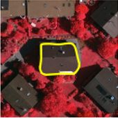
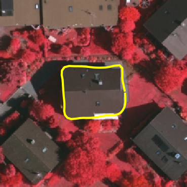
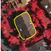
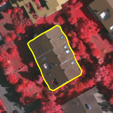
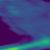
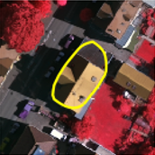
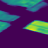
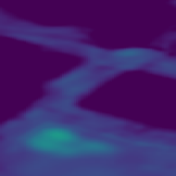
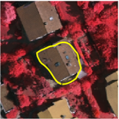
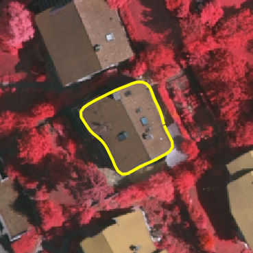
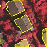
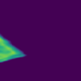
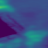
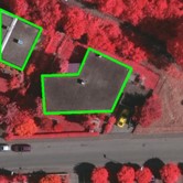
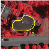
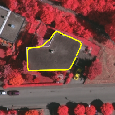
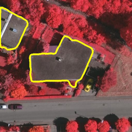
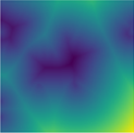
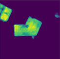
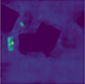
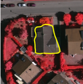
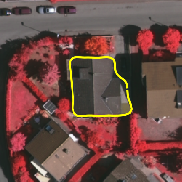
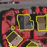
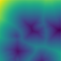
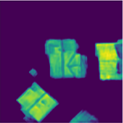
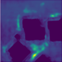
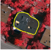
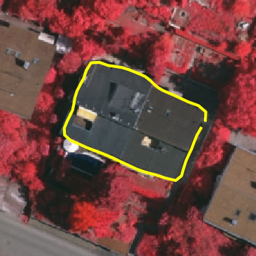
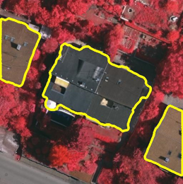
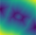
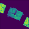
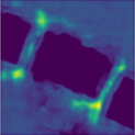
0pt

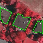
(a) Labeled Image

0pt

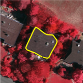
(b) DSAC

0pt

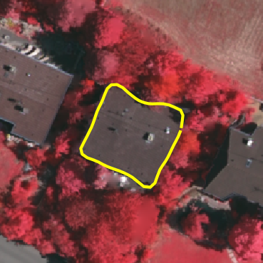
(c) DarNet

0pt

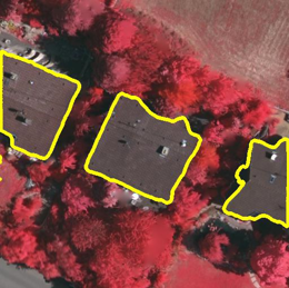
(d) Our DTAC

0pt

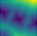
(e) Initialization

0pt

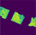
(f) $\lambda_{1}(x,y)$

0pt

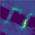
(g) $\lambda_{2}(x,y)$

Figure 9: Comparative visualization of the labeled image, the output of DSAC, the output of DarNet, and the output of our DTAC, for the Vaihingen dataset: (a) Image with label (green), (b) DSAC output, (c) DarNet output, (d) our DTAC output, (e) DTAC learned initialization map, (f) $\lambda_{1}(x,y)$ and (g) $\lambda_{2}(x,y)$ for the DTAC.

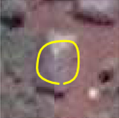
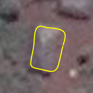
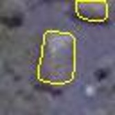
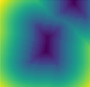
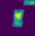
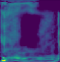
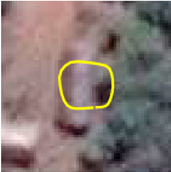
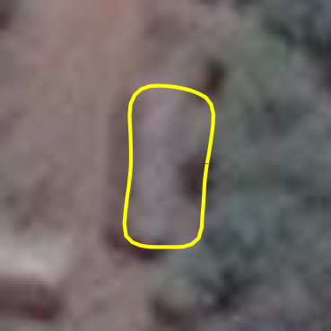
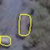
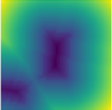
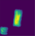
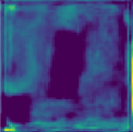
0pt

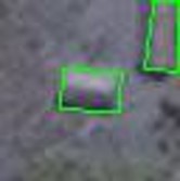
(a) Labeled Image

0pt

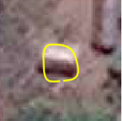
(b) DSAC

0pt

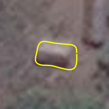
(c) DarNet

0pt

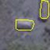
(d) Our DTAC

0pt

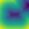
(e) Initialization

0pt

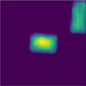
(f) $\lambda_{1}(x,y)$

0pt

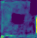
(g) $\lambda_{2}(x,y)$

Figure 10: Comparative visualization of the labeled image, the output of DSAC, the output of DarNet, and the output of our DTAC, for the Bing Huts dataset: (a) Image with label (green), (b) DSAC output, (c) DarNet output, (d) our DTAC output, (e) DTAC learned initialization map, (f) $\lambda_{1}(x,y)$ and (g) $\lambda_{2}(x,y)$ for the DTAC.

As shown in Figures 9, with the Vaihingen dataset, both the DarNet and DSAC models struggle to cope with the topological changes of the buildings and fail to appropriately capture sharp edges, while our framework readily handles these challenges in most cases. With the Bing Huts dataset, as shown in Figure 10, both the DarNet and DSAC models are able to localize the buildings, but they mainly over-segment the buildings in many cases. This may be due to their inability to distinguish the building from the surrounding soil because of the low contrast and small size of the image. Comparing the segmentation output of DSAC (Figure 10b), DarNet (Figure 10c), and DTAC (Figure 10d), our DTAC model performs well in a low contrast dataset, producing more accurate boundaries than the earlier models.

Method		Vaihingen				Bing Huts
Approach	Backbone	Dice	mIoU	WCov	BoundF	Dice	mIoU	WCov	BoundF
FCN	UNet	81.00	69.10	72.40	34.20	71.58	58.70	65.70	40.60
FCN	ResNet	80.10	67.80	70.50	32.50	74.20	61.80	66.59	39.48
FCN	Mask R-CNN	82.00	72.20	73.50	29.80	76.12	63.40	0.7051	0.7041
FCN	Ours	89.30	81.00	82.70	49.80	75.23	60.31	72.41	41.12
DTAC, Const $\lambda$	Ours	90.80	83.30	83.90	47.20	81.19	68.34	75.29	44.61
DTAC	Ours	95.20	91.10	91.71	69.02	83.24	71.30	78.45	48.49

Table 8: Model Evaluations of DTAC and others: Multiple Instance Segmentation.

Multiple Instance Segmentation

We now compare the performance of DTAC against popular models such as Mask R-CNN for multiple instance segmentation of all buildings in the Vaihingen and Bing Huts datasets. Our extensive benchmarks confirm that our DTAC model comfortably outperforms Mask R-CNN and other method by a wide margin as reported in Table 8. Although Mask R-CNN seems to be able to fairly localize the building instances, the fine-grained details of boundaries are lost, as is attested by the BoundF metric. The performance of other CNN-based approaches follow the same trend in our benchmarks.

Local and Fixed Weighted Parameters

To validate the contribution of the local weighted parameters in the level-set ACM, we also trained our DTAC on both the Vaihingen and Bing Huts datasets by allowing just a single trainable scalar parameter, constant over the entire image, for both $\lambda_{1}$ and $\lambda_{2}$. As presented in Table 7, for both the Vaihingen and Bing Huts datasets, this “constant-$\lambda$” formulation (the Chan-Vese formulation [17; 73]) still outperforms the baseline CNN in most evaluation metrics for both single-instance and multiple-instance buildings, thus establishing the effectiveness of the end-to-end training of our DTAC. Nevertheless, the DTAC with its full $\lambda_{1}(x,y)$ and $\lambda_{2}(x,y)$ maps outperforms this constant-$\lambda$ version by a wide margin in all experiments and metrics. A key metric of interest in this comparison is the BoundF score, which elucidates that our local formulation captures the details of the boundaries more effectively by locally adjusting the inward and outward forces on the contour. Figure 11 shows that our DTAC has perfectly delineated the boundaries of the building instances. However, the DTAC hobbled by the constant-$\lambda$ formulation has over-segmented these instances.

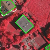
(a) Labeled Image

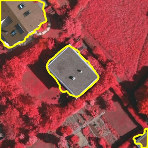
(b) DTAC, constant $\lambda$s

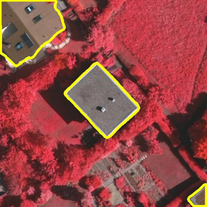
(c) DTAC

(d) $\lambda_{1}(x,y)$

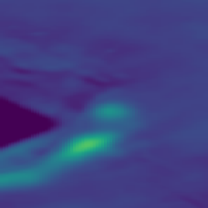
(e) $\lambda_{2}(x,y)$

Figure 11: Visualization of DTAC’s learned feature maps. (a) Labeled image. (b) DTAC output with constant weighted parameters. (c) DTAC output. (d),(e) Learned parameter maps $\lambda_{1}(x,y)$ and $\lambda_{2}(x,y)$.

4 Number of Iterations

The direct learning of an initialization map as well as its efficient end-to-end implementation have enabled the DTAC to require a significantly lower number of iterations to converge with a better chance of avoiding the undesirable local minima. As illustrated in Figure 12a, we have extensively investigated the effect of the number of iterations on the overall mIoU for both Vaihingen and Bing datasets, and our results show that DTAC exhibits a robust performance after a certain threshold. Therefore, we have chosen a fixed number $N=60$ iterations for optimal performance, which runs in less than one second in TensorFlow.

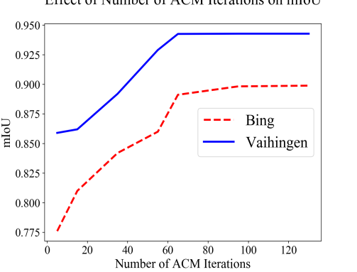
(a)

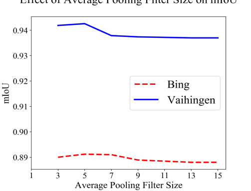
(b)

Figure 12: The effects of (a) varying the number of ACM iterations on mIoU and (b) varying the average pooling filter size on mIoU.

5 Average Pooling Filter Size

The average pooling filter size is an important hyper-parameter in the extraction of localized image statistics. As illustrated in Figure 12b, we have investigated the effect of the average pooling filter size on the overall mIoU for both Vaihingen and Bing datasets. Our experiments indicate that filter values that are too small are sub-optimal while excessively large values defeat the benefits of the localized formulation. Consequently, we set a filter size of $f=5$ for the DTAC.

6 Few-Shot Semantic Segmentation

In this section, we empirically study the models developed in Chapter 4.

1 Datasets

To evaluate SegAVA, we used the PASCAL VOC 2012 [32] dataset, which consists of 20 categories that are divided equally into 4 partitions, with 5 categories in each partition. We trained our model on 3 partitions and evaluated on the remaining partition with cross-validation.

2 Evaluation Metrics

To evaluate SegAVA’s performance, we utilized the mean Intersection over Union (mIoU) metric to measure the intersection over the union for each foreground class and took the average result over all the classes. The IoU score measures the overlap of two objects by calculating the ratio of intersection over union according to

$$\text{IoU}(G,Y)=\frac{|G\cap Y|}{|G\cup Y|},$$ (5)

where $G$ denotes the ground truth mask and $Y$ denotes the prediction mask.

3 Implementation Details

We have implemented SegAVA in Pytorch. Like [122], we used a VGG16 network [113] pretrained on ImageNet [106] as our feature extractor in the image space, and resized the input images to $417\times 417$ pixels and randomly augmented them using horizontal flipping. All the training and testing was performed on an Nvidia Titan RTX GPU, and an Intel® Core™ i7-7700K CPU @ 4.20GHz.

We trained our model for 150,000 iterations with a batch size of 2 and a stochastic gradient descent algorithm with an initial learning rate of 0.001 and a momentum value of 0.09 and weight decay of 0.0005. The learning rate was reduced by a factor of 10 in every 10,000 iterations. To determine the value of hyper-parameter $\gamma$ in (7), we performed a grid search from minimum to maximum values of $0.5$ and $4$ for $\gamma$, stepping by $0.5$, and our experiments confirmed that using $\gamma=0.5$ provides the optimal balance between the two loss terms.

4 Evaluation

Method	1-shot					5-shot
	part-1	part-2	part-3	part-4	Mean	part-1	part-2	part-3	part-4	Mean	$\Delta$
OSLSM [108]	33.6	55.3	40.9	33.5	40.8	35.9	58.1	42.7	39.1	43.9	3.1
co-FCN [101]	36.7	50.6	44.9	32.4	41.1	37.5	50.0	44.1	33.9	41.4	0.3
SG-One [135]	40.2	58.4	48.4	38.4	46.3	41.9	58.6	48.6	39.4	47.1	0.8
AMP [110]	41.9	50.2	46.7	34.7	43.4	41.8	55.5	50.3	39.9	46.9	3.5
Meta-Seg [15]	42.2	59.6	48.1	44.4	48.6	43.1	62.5	49.9	45.3	50.2	1.6
MDL [31]	39.7	58.3	46.7	36.3	45.3	40.6	58.5	47.7	36.6	45.9	0.6
PANet-init [122]	30.8	40.7	38.3	31.4	35.3	41.6	52.7	51.68	40.8	46.7	11.4
$\text{OS}_{\text{Adv}}$ [129]	46.9	59.2	49.3	43.4	49.7	47.2	58.8	48.8	47.4	50.6	0.9
Feat Weight [Nguyen et al., 2019]	47.0	59.6	52.6	48.3	51.9	50.9	62.9	56.5	50.1	55.1	3.2
PANet [122]	42.3	58.0	51.1	41.2	48.1	51.8	64.6	59.8	46.5	55.7	7.6
SegAVA	44.1	59.8	52.9	45.6	50.6	51.9	65.1	60.2	47.2	56.1	5.5

Table 9: Results from SegAVA for 1-way, 1-shot and 1-way, 5-shot segmentation on the PASCAL-5i dataset using mean IoU as the measure of accuracy. $\Delta$ represents the difference between the 1-shot and 5-shot means.

1-Way, 1-Shot and 5-Shot Segmentation

As detailed in Table 9, our experiments for the tasks of 1-way 1-shot and 1-way 5-shot semantic segmentation demonstrates competitive performance on the PASCAL-5i dataset. For 1-way, 5-shot segmentation, our model achieves a new state-of-the art performance and consistently outperforms competing approaches such as PANet [122] and $\text{OS}_{\text{Adv}}$ [129], except for part-4. For 1-way, 1-shot segmentation, we have achieved state-of-the-art results on part-2 and part-3 while also being competitive to Feat Weight [94] with respect to the overall mean. Our qualitative results (Figure 13) show that single or multiple instances belonging to the same class have been appropriately segmented.

Annotations	SegAVA		PANet
	1-shot	5-shot	1-shot	5-shot
Dense	50.6	56.1	48.1	55.7
Scribble	46.9	55.3	44.8	54.6
Bounding box	47.2	53.5	45.1	52.8

Table 10: Comparison between SegAVA and PANet in semi-supervised segmentation. Results are expressed in mean-IoU.

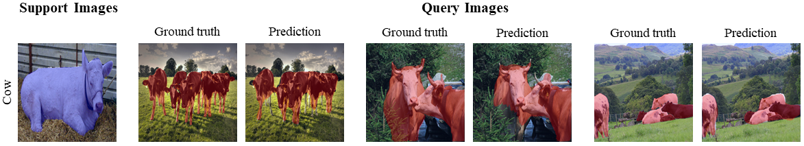
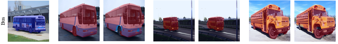
Figure 13: Example results from evaluating SegAVA in 1-way, 1-shot segmentation on the PASCAL-5i dataset.

5 Semi-Supervised Segmentation

We have also validated the effectiveness of our SegAVA by using bounding box and scribble annotations. As reported in Table 10, our model generalizes well when using these weaker types of annotations, and is still able to extract the important features of the support set and localize and segment the objects of interest in the query images. For the task of 1-way, 5-shot segmentation, the performance of our model using scribble annotations is surprisingly close to when dense level masks are made available. Our model outperforms PANet in all tasks using both types of weaker annotations. Qualitative results for semi-supervised segmentation are shown Figure 14.

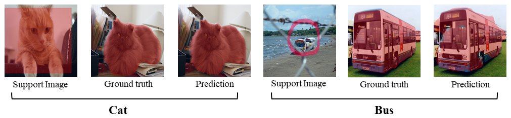
Figure 14: Example results from SegAVA on 1-way, 1-shot segmentation using both bounding boxes and scribble annotations.

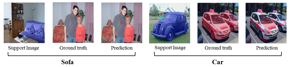
Figure 15: Example of failure cases from evaluating SegAVA in 1-way, 1-shot segmentation on the PASCAL-5i dataset.

6 Failure Cases

Figure 15 shows example failure cases of our model. First, in some instances, our model is unable to fully delineate the segmentation masks and may additionally produce undesired patches. This can be resolved by incorporating post-processing methods. Second, the model is unable recognize some cases, which may be due to the extracted features in the image or latent space being insufficient for certain classes.

7 Active Contour Assisted Few-Shot Segmentation

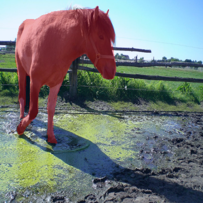
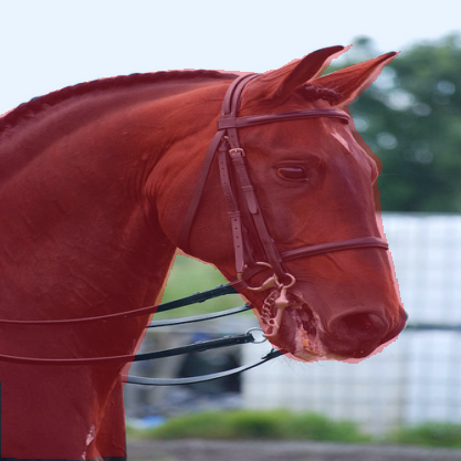
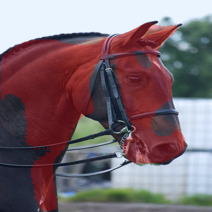
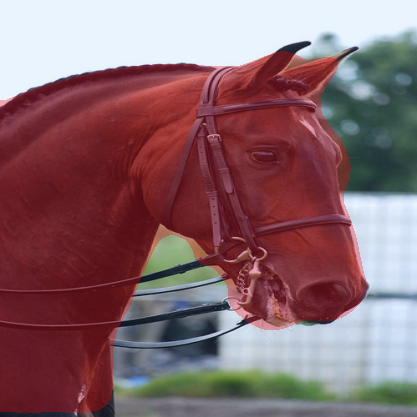
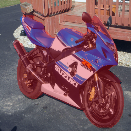
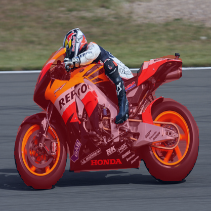
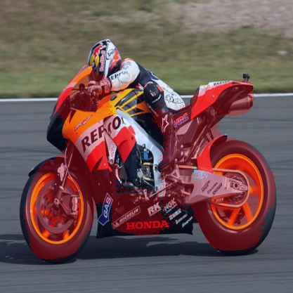
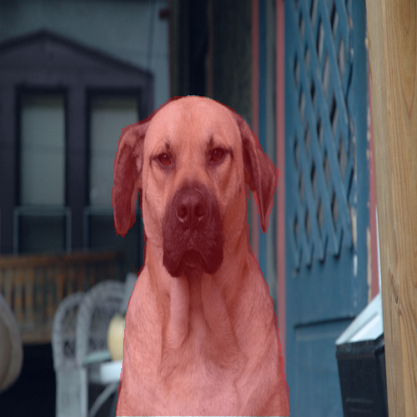
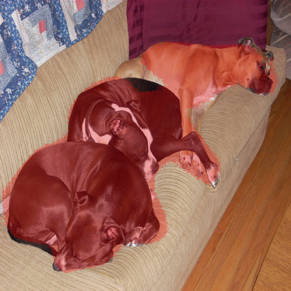
(a) (b) (c) (d)

Figure 16: Qualitative comparison of SegAVA and SegAVA+DALS. (a) Support Image. (b) Groundtruth. (c) SegAVA. (d) Combined. Qualitative comparison of SegAVA and SegAVA+DALS for 1-way, 1-shot and 1-way, 5-shot segmentation tasks on the PASCAL-5i dataset. Combined denotes a model that consists of SegAVA as the backbone and DALS as a post-processor.

Model	1-shot	5-shot
SegAVA	50.6	56.1
Combined	52.0	57.3

Table 11: Quantitative comparison of SegAVA and SegAVA+DALS for 1-way, 1-shot and 1-way, 5-shot segmentation tasks on the PASCAL-5i dataset. Combined denotes a model that consists of SegAVA as the backbone and DALS as a post-processor.

We further leveraged our proposed DALS framework along with SegAVA to delineate and refine the initial segmented boundaries. Quantitative comparisons, as presented in Table 11, demonstrate the benefits of leveraging DALS as post-processor with SegAVA. For 1-way, 1-shot and 1-way, 5-shot segmentation tasks, the combined framework has improved the overall mIoU by 1.4% and 1.2%, respectively.

Figure 16 shows the qualitative comparison between SegAVA and the combined framework with DALS. Evidently, DALS delineates the mis-segmented regions and improves the segmentation accuracy around the edges.

Chapter 6 Conclusions and Future Work

1 Conclusions

This thesis has contributed several novel, fully automatic image segmentation pipelines that can robustly produce precise object and region boundaries and semantic segmentation masks, and learn to do so from limited amounts of training data both in supervised and semi-supervised, few-shot learning settings.

Motivated by the shortcomings of CNNs in tasks requiring segmentation predictions with precise boundaries, we first proposed an end-to-end, edge-aware model for semantic segmentation. Our network explicitly accounts for object edge information by using a dedicated shape stream that processes the feature maps at the boundary level and fuses the multiscale contextual information of the boundaries with the encoder output of the regular segmentation stream. Additionally, edge-aware loss functions emphasize the learning of edge information during training by tuning the weights of the downstream encoder and regularizing the network to prioritize boundaries. We validated the effectiveness of our approach on the task of brain tumor segmentation using the BraTS 2018 dataset. The results indicate that our network produces more accurate segmentation outputs with fine-grained boundaries in comparison to the popular segmentation networks U-Net and V-Net.

Second, we built upon the notion of edge-aware networks and proposed an end-to-end volumetric (3D) edge-aware framework for the reliable and automated segmentation of kidneys and kidney tumors. Our network consists of a an encoder-decoder architecture equipped with a boundary stream that processes the edge information separately and is supervised by edge-aware losses. We have validated the effectiveness of our approach by training and testing our model on 2019 MICCAI KiTS Kidney Tumor Segmentation Challenge dataset. Our method achieved dice scores of $0.9742$ and $0.8103$ for kidney and tumor repetitively and an overall composite dice score of $0.8923$ and ranks 9th overall in terms of composite dice among the 100 participants of this challenge.

Third, we introduced the EG-CNN, a plug-and-play module for boundary-aware CNN segmentation, which can be paired with an existing encoder-decoder architecture to improve the segmentation accuracy. Our EG-CNN does not require any additional annotation effort since edge information can be extracted from the ground truth segmentation masks. Supervised by edge-aware and consistency loss functions, the EG-CNN learns to emphasize the edge representations by leveraging the feature maps of intermediate resolutions in the encoder of the main stream and feeding them into a series of edge-gated layers. We evaluated the EG-CNN against three popular 3D segmentation architectures, U-Net, V-Net, and Seg-Net, in the tasks of brain and kidney tumor segmentation on the BraTS19 and KiTS19 datasets. Our results indicate that the addition of the proposed EG-CNN consistently improves the segmentation accuracy in all the benchmarks.

We then turned out attention taking advantage of the automated, data-driven nature of CNNs and the precision and versatility of ACMs to devise a powerful image segmentation pipeline.

We first presented Deep Active Lesion Segmentation (DALS), a novel framework that combines the capabilities of the CNN and the level-set ACM to yield a robust, fully automatic medical image segmentation method that produces more accurate and detailed boundaries compared to competing state-of-the-art methods. The DALS framework includes an encoder-decoder that feeds a level-set ACM with per-pixel parameter functions. We evaluated our framework in the challenging task of lesion segmentation with a new dataset, MLS, which includes a variety of images of lesions of various sizes and textures in different organs acquired through multiple imaging modalities. Our results affirm the effectiveness our DALS framework.

Second, we introduced a novel image segmentation framework, called DTAC, which is an end-to-end trainable unification of ACMs and CNNs. For this purpose, we proposed a new locally-penalized Eulerian energy model that includes pixel-wise learnable parameters that can adjust the contour to precisely capture and delineate the boundaries of objects of interest in the image. We tackled the problem of building instance segmentation on two challenging datasets, Vaihingen and Bing Huts, as test cases and our model significantly outperforms the current state-of-the-art method, DarNet. Furthermore, unlike DarNet and DSAC, which rely on the manual initialization of ACM contours, our model is fully automatic, as its backbone CNN learns initialization maps as well as weighted parameters that can guide the contour to avoid suboptimal solutions. Moreover, DarNet and DSAC are limited to segmenting a single building at a time, whereas our DTAC can segment multiple buildings simultaneously. In view of the level of success that DTAC has achieved in this application and the fact that it features a general Eulerian ACM formulation, it seems readily applicable to other segmentation tasks in various domains, wherever purely CNN filter-based approaches can benefit from the versatility and precision of ACMs in delineating object boundaries in images.

Finally, we addressed semi-supervised learning of image segmentation models, particularly the challenging problem of few-shot segmentation by feature alignment in the image and latent spaces of support and query samples. Our SegAVA model leverages a latent stream as well as an encoder-decoder stream to extract the most essential discriminative semantic embeddings and learns similarities in both spaces. The latent stream consists of two variational autoencoders, conditioned on the support and query sets, that jointly learn to generate the input images and discriminatively identify the most common class-specific representations using a Wasserstein-2 metric. These embedding are then decoded to the image space and concatenated with common representation that are found by comparing support and query extracted features using our fully convolutional decoder. We trained and tested SegAVA using the PASCAL-5i dataset, demonstrating new state-of-the-art performance in 1-shot and 5-shot scenarios. We also validated the SegAVA model in a semi-supervised setting where only bounding boxes are provided, and our results demonstrate the sustained effectiveness of our approach.

2 Future Work

The research presented in this thesis can be further developed along the following avenues:

1. Edge-aware networks can be further studied by adding modules that assist the boundary stream better to delineate and find the representations that correspond to the edges. In particular, a module such as the proposed differentiable level-set ACM can be added to each stage of the boundary stream to further refine the edges. Since the ACM part is capable of back-propagating error, the entire framework can be trained in an end-to-end manner.

   Additionally, notion of fusing the output of the boundary stream and main stream can be further studied and developed. In this work, we presented a simple yet effective scheme for our fusion module, with an emphasis on reducing the number of free parameters. However, future efforts can include fusing the output of each stage of the boundary and main streams in multiple resolutions to ensure the capture of fine-grained details.

   Finally, the end-to-end trainable active contours can be extended to volumetric applications in order to interact with 3D encoder-decoders, which are pervasive in medical image analysis. The efficiency of the proposed framework is a noteworthy factor in such integration as previous 3D ACM methods were prohibitively expensive computationally and as a result have not been extensively utilized in medical imaging to date.

2. End-to-end trainable deep active contours were leveraged in a supervised learning setting. However, given the fact that ACMs usually do not require training labels, an intriguing research direction is to utilize the proposed framework in semi-supervised or unsupervised setting. Different levels of supervision can be employed in initializing the contour. For instance, starting from a bounding box that identifies a rough estimate of the target region, the trainable ACM can be leveraged to fully delineate the segmentation mask.

   Another important research direction for trainable deep active contours is interactive segmentation and active learning where a user may provide additional input and correct the mistakes of the segmentation model as necessary, from which the model can learn.

3. A promising direction for our SegAVA framework is to study the synergy between it and other segmentation techniques in which the user can interactively provide additional supervision, whether in the form of mouse clicks or bounding boxes/scribbles, to improve the accuracy of the segmentation. Additionally, our end-to-end trainable active contours is a promising candidate for integration with SegAVA.

   Another important direction is to study additional modules that can be utilized along with SegAVA to provide the means for cross-domain, few-shot segmentation. This may be realized by leveraging additional transformation layers to accommodate domain shift and various feature distributions.

   Finally, applications such as medical image analysis, where establishing dense, pixel-wise annotated datasets is very costly, can benefit from our SegAVA model.

Chapter 7 Fast and Automatic Segmentation of Pulmonary Lobes from Chest CT Using a Progressive Dense V-Network

The material in this appendix was published as [58], which is an expanded version of the publication [59].

Appendix 7.A Abstract

Automatic, reliable lobe segmentation is crucial to the diagnosis, assessment, and quantification of pulmonary diseases. Existing pulmonary lobe segmentation techniques are prohibitively slow, undesirably rely on prior (airway/vessel) segmentation, and/or require user interactions for optimal results. We introduce a reliable, fast, and fully automated lung lobe segmentation method based on a Progressive Dense V-Network (PDV-Net). The proposed method can segment lung lobes in one forward pass of the network, with an average runtime of 2 seconds using a single Nvidia Titan XP GPU. An extensive robustness analysis of our method demonstrates reliable lobe segmentation of both healthy and pathological lungs in CT images acquired by scanners from different vendors, across various CT scan protocols and acquisition parameters.

Appendix 7.B Introduction

Human lungs are divided into five lobes. The inner membrane of the lung (visceral pleura) folds towards the center of the lung and creates double layer fissures that define the five lobes. The lobar boundaries are made of two major (oblique) fissures and a minor (horizontal) fissure. As shown in Figure 1, the left lung has two lobes separated by a major fissure—the upper (superior) lobe and the lower (inferior) lobe. Along with upper and lower lobes, the right lung has a middle lobe; a major fissure separates the upper lobe from the middle lobe and a minor fissure separates the lower lobe from the middle lobe. Each of the five lobes is functionally independent, with its own bronchial and vascular systems.

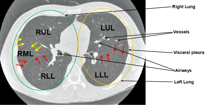
Figure 1: An axial lung CT slice with visible fissures. The left upper lobe (LUL) and left lower lobe (LLL) are defined by a major fissure (indicated by red arrows); the right upper lobe (RUL), right middle lobe (RML), and right lower lobe (RLL) are defined by a major fissure (indicated by red arrows) and a minor fissure (indicated by yellow arrows).

Automatic segmentation of the lung lobes is important for both clinical and technical purposes. From the clinical perspective, automatic lung lobe segmentation can help radiologists review chest CT scans more efficiently. This is because radiologists often report their pulmonary findings by indicating the affected lung lobe, whose identification requires them to navigate through the nearby slices and search for fissure lines, which are often visually indistinct. Automatic lung lobe segmentation can eliminate the need for such a tedious and time-consuming process. From the technical perspective, accurate lung lobe segmentation can assist several subsequent clinical tasks, including nodule malignancy prediction (cancers mostly occur in the left or right upper lobes), automatic lobe-aware report generation for each nodule (see Figure 2(a)), and assessment and quantification of chronic obstructive pulmonary diseases (COPD) and interstitial lung diseases (ILD), by narrowing down the search space to the lung lobes most-likely to be affected.

However, identifying fissures poses a challenge for both human and machine perception. First, fissures are most often incomplete, not extending to the lobar boundaries. This is shown in Figure 2(a) where the horizontal fissure is incomplete, unlike the oblique fissures. Several studies in the literature have confirmed the incompleteness of fissures as a very common phenomenon. After reviewing 100 fixed and inflated lung specimens, Raasch et al. [100] found incomplete right major fissures in 70% of the cases, left major in 46% of the cases, and 94% across the minor fissures. Moreover, the studies of Gulsun et al. [40] and Aziz et al. [5] also showed more than 50% incompleteness in pulmonary fissures. Second, the visual characteristics of lobar boundaries change in the presence of pathologies. The changes could also be related to their thicknesses, locations, and shapes. Third, there also exist other fissures in the lungs that can be misinterpreted as the major and minor fissures that separate the lobes. Examples include accessory fissures (see the sagittal slice in Figure 2(c)) and azygos fissures (see the axial slice in Figure 2(d)).

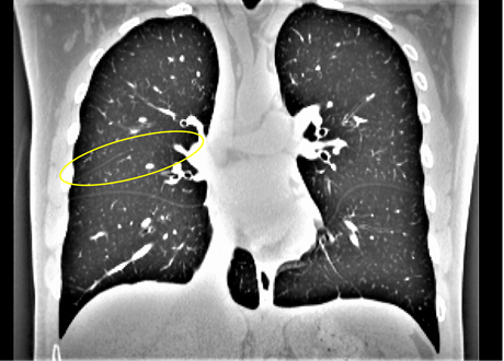
(a)

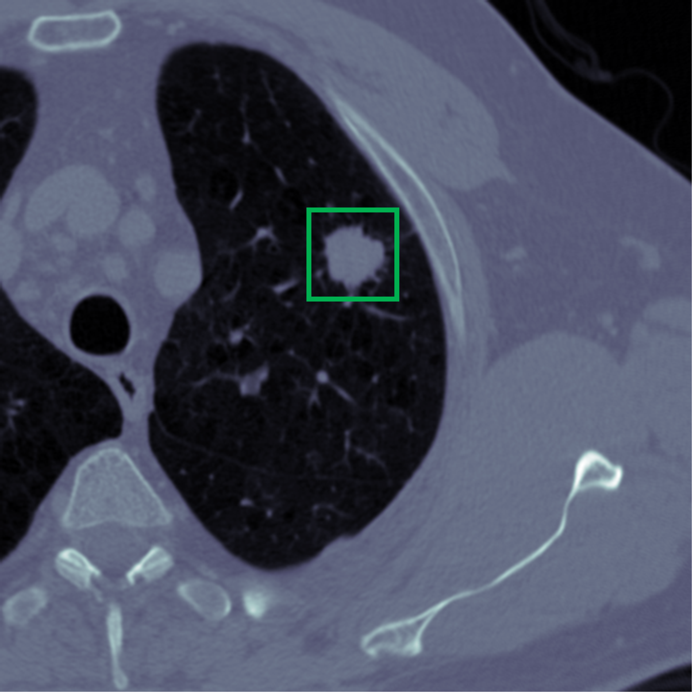
(b)

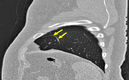
(c)

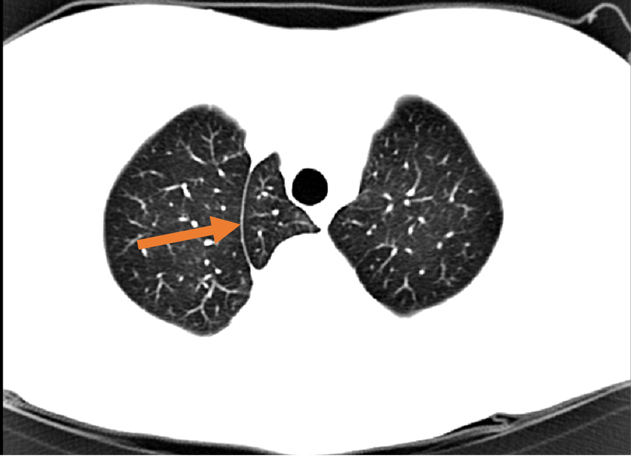
(d)

Figure 2: (a) A coronal slice where the major fissures are complete and visible, but the minor fissure (circled) is incomplete. (b) Nodule shown in the bounding box. (An example nodule report: 5mm nodule found in the left upper lobe). (c) Accessory fissure (arrows) in a left lung sagittal slice, which looks similar in shape to a minor fissure. (d) Azygos fissure (arrow) in an axial slice creates an extra lobe (azygos lobe) in the right lung

To address the need for accurate and robust lobe segmentation, we have pursued a fully automatic and reliable deep learning solution based on a Progressive Dense V-Network (PDV-Net) [59]. Our PDV-Net model inputs an entire CT volume and generates accurate segmentation of the lung lobes in about 2 seconds in only a single forward pass of the network, eliminating the need for any user interaction or any prior segmentation of the lungs, vessels, or airways, which are common assumptions in the design of existing models. Extensive robustness analyses demonstrate that our proposed method performs reliably for CT scans acquired using various imaging protocols from both healthy and pathological patients.

Appendix 7.C Related Work

There have been several efforts to segment lung lobes using semi-automatic and automatic techniques. We categorize these approaches into two groups: reliant approaches, which rely on a prior segmentation or anatomical information, and non-reliant approaches, which do not rely on such prior segmentations.

1 Reliant Approaches

Prior-Based Segmentation

Reliant approaches require as input a segmentation mask of lungs or lobes (different modalities), airways and vessels, or fissure initialization. A good example of the latter is the work by Doel et al. [29], in which lobe segmentation is performed based on an initialization via fissure detection. In another example of fissure initialization, Iwano et al. [61] proposed semi-automatic and automatic lobe segmentation methods based on region-growing. The semi-automatic approach requires major and minor fissure initialization, whereas for the automatic approach, recognition of lobar bronchi and localization of fissures are performed prior to the final lobar segmentation. On average, the semi-automatic approach takes approximately 80 seconds and the automatic approach takes approximately 44 seconds per case.

A number of works depend on prior segmentation of airways, vessels, or fissures. The work by Bragman et al. [12] is a good representative, wherein the suggested method relies on the prior segmentation of airways and vessels. Specifically, a population model of fissure priors was constructed and combined with patient-specific anatomical information for non-parametric surface fitting. Despite the promising results, the model lacks robustness and its reliance on prior knowledge limited the study. In recent work, Giuliani et al. [39] proposed an approach to segment lobes from an approximate segmentation based on the airway tree. The final lobe segmentation was generated by combining the approximate segmentation with all the lung structures (airways, vessels, lungs, and fissures) segmentation using a multilevel graph cut algorithm. This segmentation method is highly reliant on the quality of the prior airway and vessel segmentations, as well as anatomical knowledge. Lassen and van Rikxoort [74] proposed a watershed-based lobe segmentation method by combining anatomical information from lungs, fissures, vessels, and bronchi. Despite reporting improved segmentation in the presence of incomplete fissures, the failure of individual prior segmentations limited the performance of the overall segmentation. Based on this work, Lassen-Schmidt et al. [75] proposed an interactive lobe segmentation method to interactively correct lobe segmentation error through user inputs. However, this improvement was obtained at the price of prolonged segmentation sessions. Lim et al. [79] performed quantification of emphysema in 66 patients with moderate to severe emphysema who had undergone CT for lung volume reduction planning. They used lobar segmentation from four different prototypes for inter-software variability in lobe-wise emphysema quantification. Although the lobe segmentation performance is not reported, it is dependent on prior airway and vessel segmentation.

Other works also rely on prior lung or lobe segmentation masks. For example, Bauer et al. [9] segmented the lung lobes in the expiration phase based on a prior lobe segmentation mask obtained from a CT image acquired in the inspiration phase. An automated lung and lobe segmentation pipeline was proposed by Blaffert et al. [11], in which a lung model mesh based on watershed segmentation is adapted to lobar segmentation. Final lobe regions are obtained by adjusting based on overlaid lungs in a post-processing step. However, the authors do not report a quantitative evaluation of lobar segmentation. The model takes 20 seconds to perform lobar segmentation in each CT scan.

Atlas-Based Segmentation

Another variation of reliant segmentation is registration using mutual information with a previously segmented atlas. The performance of final lobe segmentation is greatly dependent on the performance of the segmentation algorithm used in creating a reference atlas. Among atlas-based approaches for lobe segmentation, Ross et al. [104] employed the thin-plate spline and a maximum a posteriori estimation method using a manually-defined atlas as a reference. Fissure points were selected based on the atlas and the final lobe segmentation was generated after a post-processing step. Although this method did not rely on any prior airway and vessel segmentation, the execution time was long. Moreover, the creation of the atlas is very cumbersome and prone to poor results in pathological lung cases. By contrast, Pu et al. [99] performed lobe segmentation by fitting an implicit function to fissures without reliance on prior airway or vessel segmentation. Although they achieved good accuracy for healthy lungs, the performance of their method degraded in the case of lungs with abnormal orientations. Unlike the other atlas-based segmentations, van Rikxoort et al. [120] made use of multiple atlases for lobe segmentation. Their method showed promise albeit at the expense of slow execution.

2 Non-Reliant Segmentation

Recently, a few convolutional neural-network-based lobe segmentation techniques have been proposed [36; 33; 124]. The segmentation method of George et al. [36] employs a 2D fully convolutional network followed by a 3D random walker algorithm. This approach does not rely on a prior segmentation of airways or vessels nor on any pre-computed atlases; however, it cannot generate lobe segmentation in a single pass, nor in an end-to-end manner. Furthermore, the 3D random walker algorithm relies on a number of heuristics for the initialization of seeds and weights. Ferreira et al. [33] proposed a lobe segmentation model based on a fully regularized V-Net model with deep supervision and carefully chosen regularization. Although the performance looks impressive, the model was trained with few examples, so it lacks generalizability and may not be effective for varying CT scan cases. A 3D Dense Net-based lobe segmentation method was proposed by Wang et al. [124]. Although they reported good accuracy for pathological lungs, their lobe segmentation method relies on prior lung segmentation and assumes the presence of five lobes, which might not always be the case (e.g., [81]).

Our work [59] mitigates the aforementioned limitations—namely, reliance on prior masks, slow runtime, and lack of robustness—through an end-to-end learning network. Without relying on any prior airway/vessel segmentation or anatomical knowledge or atlases, our method performs lobe segmentation in a single pass of the network. Owing to the full utilization of the 3D context in our model, the resulting lobe segmentation is smooth and nearly noise-free, which eliminates the need for any subsequent post-processing to fill holes or remove noisy patches from outside the lung area. Our method shows promise for the potential clinical use in quantification of pulmonary diseases and automatic generation of radiological reports.

Appendix 7.D Materials and Methods

1 Progressive Dense V-Net

Combining ideas from dense V-Networks [38] and progressive holistically-nested networks [43], we propose a new architecture—the Progressive Dense V-Network (PDV-Net), an end-to-end solution for organ segmentation in 3D volumetric data.

As shown in Figure 3, the input to the network is first down-sampled and concatenated with a strided $5\times 5\times 5$ convolution of the input with 24 kernels. The concatenation result is then passed to 3 dense feature blocks, each consisting of 5, 10, and 10 densely-wired convolution layers respectively. The growth rates of the dense blocks are set to 4, 8, and 16 respectively. All the convolutional layers in a dense block have a kernel size of $3\times 3\times 3$ and are followed by batch normalization and parametric rectified linear units (PReLU). The outputs of the dense feature blocks are consecutively utilized in low and high resolution passes via convolutional down-sampling and skip connections. This enables the generation of feature maps at three different resolutions. The outputs of the skip connections of the second and third dense feature blocks are further up-sampled in order to be consistent with the size of the output in the first skip connection. The feature maps from skip1 are passed to a convolutional layer followed by a softmax, which outputs the probability maps. In the second pathway, the feature maps from skip1 and skip2 are merged and the output probability maps are produced by a convolutional layer followed by softmax. Similarly, we obtain the final segmentation resulting from the merged feature maps resulted from the skip2 and skip3 connections. Unlike the dense V-Net, the PDV-Net generates the final output by progressively improving the outputs from the previous pathways.

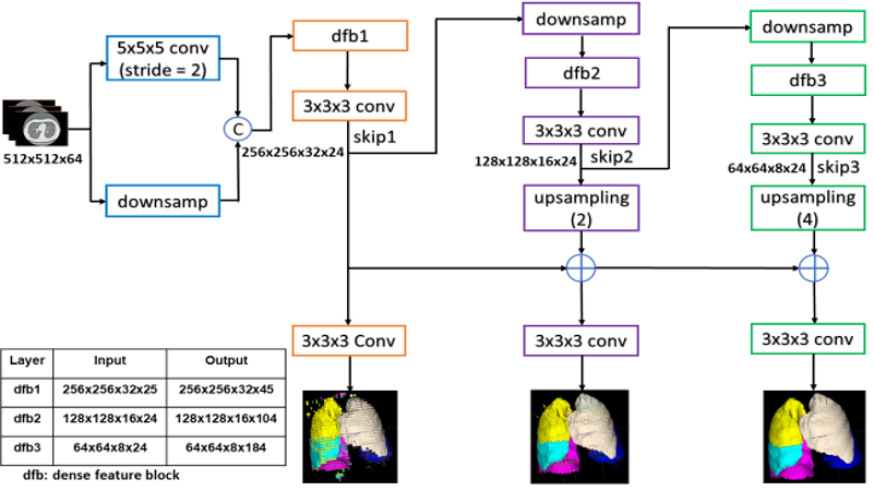
Figure 3: PDV-Net model for the segmentation of lung lobes. Segmentation outputs in different pathways are progressively improved for the final result.

The PDV-Net is trained using a subset $S$ of a volumetric medical image dataset $(\mathcal{D})$. The training set $(S)$ contains 3D CT scan images and their corresponding ground truth labels. So, $S=(\mathcal{X}_{n},\mathcal{Y}_{n})$, for $n=1,\dots,N$, where the input volumes $\mathcal{X}_{n}^{(m)}={x_{i}^{(n)};i=1,\dots|\mathcal{X}|_{n}}$, and the corresponding ground truth labeled volumes $\mathcal{Y}_{n}^{(m)}={y_{i}^{(n)}}$ $i=1,\dots|\mathcal{Y}|_{n},y_{l}^{(n)}\in\{0\dots L\}$. Here, $|S|$ is the total number of training examples passed to the network and $L$ is the number of labels provided in the ground truth data through per-voxel labeling $(l)$. To train the PDV-Net, we use a Dice loss function [87] at each level of the progressive network, which directly maximizes the similarity between the predicted values and the ground truth over all voxels. This loss properly handles the class imbalance problem prevalent in lung lobe segmentation: lung lobes have different sizes and background regions can be large. We employ a multi-class Dice for the segmentation task:

$$d=\sum_{l=1}^{L}\frac{\sum_{j=1}^{Z}p_{j}^{l}g_{j}^{l}}{\sum_{j=1}^{Z}(p_{j}^{l})^{2}+\sum_{j=1}^{Z}(g_{j}^{l})^{2}},$$ (1)

where $Z$ is the total number of voxels, $L$ is the number of classes, $p_{j}^{l}$ denotes the predicted probabilities for each class, and $g_{j}^{l}$ denotes the corresponding ground truth for each class.

2 Data

We used 3 public datasets to evaluate our model:

1. We selected a subset of chest CT volumes (354 cases) from the LIDC dataset [3] for annotation. To ensure variation in the data, the CT scans were selected such that both challenging and visible fissures are well-represented in the dataset. The lobe segmentation ground truth masks were generated in a semi-automatic fashion by multiple human annotators using the chest imaging platform feature of 3D Slicer. To mitigate bias in the ground truth, the generated masks were later refined and validated by an expert radiologist. The dataset was partitioned into 270 training and 84 test cases. 10% of the training set was utilized as the validation set to select values for the hyper-parameters. The CT scans used in the experiment have a variable number of slices with each CT volume containing 100 to 672 slices of size $512\times 512$ pixels. Figure 4 shows the histograms of the number of slices per volume, and of the voxel dimensions which vary between 0.49–0.98 mm, 0.49–0.98 mm, and 0.45–3.00 mm along the $x$, $y$, and $z$ axes, respectively. Therefore, the selected CT scans used for pulmonary lobe segmentation not only exhibit varying shapes of fissures and lobes, but also show a variable number of slices and voxel sizes.

2. We selected 154 CTs from the LTRC database [66]. The LTRC dataset includes lobe masks for pathological cases that have clear evidence of COPD or ILD diseases, including emphysema and fibrosis. The LTRC cases allow us to measure the robustness of our model against pathologies in the lungs.

3. We used 55 cases of the Lobe and Lung Analysis (LOLA11) challenge [81] and submitted our results to the challenge organizers for evaluation.

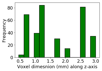
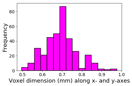
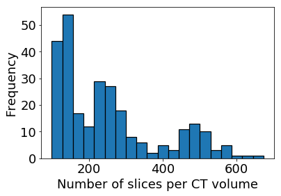
Figure 4: Histograms (from left to right) of the number of slices per volume; voxel dimensions along the $x$ and $y$ axes; and voxel dimensions along the $z$ axis of lung CT scans in the entire LIDC dataset.

Appendix 7.E Experiments

1 Baselines for Comparison

For our baseline comparison, we used a U-Net architecture [102] and a dense V-Net. The former is used in the most recent published article for lung lobe segmentation [36] and the latter is a strong baseline for comparison, which we are the first to employ for lung lobe segmentation.

2 Implementation Details

For our PDV-Net and the dense V-Net, the training volumes were first normalized, followed by rescaling to $512\times 512\times 64$, using one NVIDIA Titan XP GPU. Due to the large memory footprint of the model, the gradient check-pointing method [14] was used for memory-efficient back-propagation. Additionally, batch-wise spatial dropout [38] is incorporated for regularization purposes. The training was performed on a 64-bit Intel Xeon E5-2697 v4 2.30 GHz CPU system with 256 GB of RAM. We used the Adam optimizer [69] with a learning rate of 0.01 and a weight decay of $10^{-7}$.

For the 2D U-Net model, the implemented architecture is symmetric and consists of four contracting and expanding layers, starting with 16 features in the first layer and doubling the number of features in each step. Each contracting layer consists of two $3\times 3$ convolutions and a ReLU activation followed by a $2\times 2$ max-pooling layer. The expansion path consists of an up-convolution with feature concatenation from the respective contracting layer, and two $3\times 3$ convolutions. In addition, all the ReLU layers are preceded by a batch-normalization layer. To improve the training process, we also used a generalized Dice score as the loss function, such that the contribution of each class in the image to the gradients is balanced. We trained the network with axial slices from all the training volumes, each sized $512\times 512$ pixels and normalized to have values between 0 and 1. To avoid over-fitting to the background class, we used only the axial slices, wherein at least one lung lobe is present. We used the Adam optimizer with a learning rate of $5\times 10^{-5}$ and batches of 10 images.

Appendix 7.F Results and Discussion

1 LIDC Results

Table 1 shows the calculated overall and lobe-wise Dice scores and standard deviations for each of the models. Our PDV-Net model, with an overall score of $0.939\pm 0.020$, significantly outperformed the 2D model and yielded consistently larger Dice scores for each of the lung lobes against both the DV-Net and U-Net. Moreover, the lower standard deviation for each lobe indicates that our progressive model is more robust. Figure 5 provides a qualitative comparison between the three models, showing that our PDV-Net model captures lung fissures better than the 2D U-Net and DV-Net. The superiority of our PDV-Net model is evident both in slice (axial, coronal, sagittal) and 3D views.

Dataset	Model	RUL	RML	RLL	LUL	LLL	Overall
LIDC(84)	2D U-Net	0.908 $\pm$ 0.049	0.844 $\pm$ 0.076	0.940 $\pm$ 0.054	0.959 $\pm$ 0.042	0.949 $\pm$ 0.056	0.920 $\pm$ 0.043
	3D DV-Net	0.929 $\pm$ 0.036	0.873 $\pm$ 0.058	0.951 $\pm$ 0.018	0.958 $\pm$ 0.020	0.949 $\pm$ 0.041	0.932 $\pm$ 0.023
	3D PDV-Net	0.937 $\pm$ 0.031	0.882 $\pm$ 0.057	0.956 $\pm$ 0.017	0.966 $\pm$ 0.014	0.966 $\pm$ 0.037	0.939 $\pm$ 0.020
LTRC(154)	2D U-Net	0.914 $\pm$ 0.039	0.866 $\pm$ 0.054	0.952 $\pm$ 0.023	0.961 $\pm$ 0.023	0.954 $\pm$ 0.021	0.929 $\pm$ 0.025
	3D DV-Net	0.949 $\pm$ 0.013	0.901 $\pm$ 0.021	0.959 $\pm$ 0.009	0.961 $\pm$ 0.007	0.958 $\pm$ 0.012	0.946 $\pm$ 0.008
	3D PDV-Net	0.952 $\pm$ 0.011	0.908 $\pm$ 0.020	0.961 $\pm$ 0.008	0.966 $\pm$ 0.006	0.960 $\pm$ 0.010	0.950 $\pm$ 0.007

Table 1: Performance comparison of the proposed 3D progressive dense V-net with the 2D U-net and 3D dense V-net models in segmenting 84 LIDC and 154 LTRC cases. Mean Dice score and standard deviation for each lobe have been reported.

	Raw Slice	GT	U-Net	DV-Net	PDV-Net
Axial
Coronal
Sagittal
	3D

Figure 5: Qualitative comparison of PDV-Net’s superior performance, both in slice and volume level, against DV-Net and U-Net. Note how noisy patches and rough boundaries are removed from the final segmentation generated by the PDV-Net. Color coding: almond: LUL, blue: LLL, yellow: RUL, cyan: RML, pink: RLL.

We further used Bland-Altman plots to measure the agreement between our PDV-Net and ground truth segmentations of the 84 LIDC cases (Figure 6). Good agreement was observed between our segmentation model and ground truth in every plot (Lung and LLL being the two best agreements). Pearson correlation showed that all six volume sets in ground truth are strongly correlated with the corresponding six volume sets in the PDV-Net segmentation, with $p<0.001$.

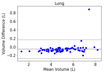
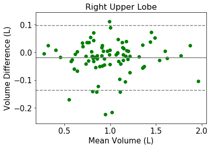
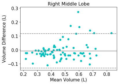
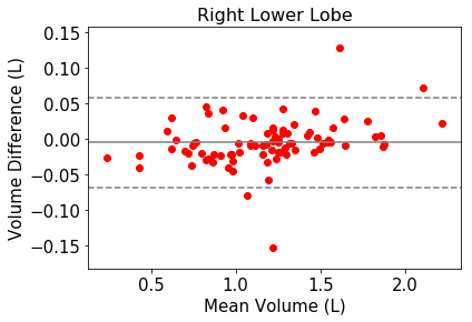
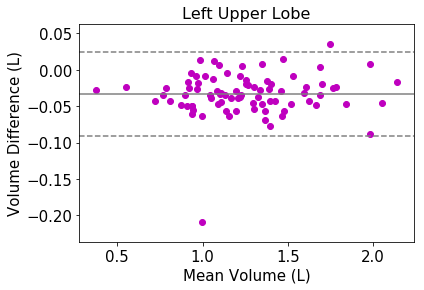
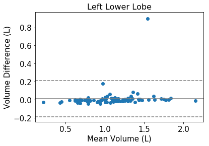
Figure 6: Bland-Altman plots show the agreement between 3D PDV-Net and ground truth.

2 LTRC Results

Table 1 shows that the 3D progressive dense V-Net achieves an average Dice score of $0.950\pm 0.007$, significantly improving the dense V-Net ($0.946\pm 0.008$). Once again, the progressive dense V-Net model outperformed the 2D U-Net model with an average Dice score of $0.929\pm 0.025$. Individual lobes were segmented better by our 3D progressive dense V-Net model than by the 3D dense V-Net and the 2D U-Net models (Table 1). Note that the LTRC dataset includes many pathological cases where the fissure lines are either invisible, distorted, or absent in the presence of pathologies such as emphysema, fibrosis, etc. As a result, lobe segmentation becomes more challenging. Nevertheless, our model performed well in segmenting lobes in pathological cases from the LTRC dataset. Moreover, our model outperformed the model of George et al. [36] in segmenting the LTRC cases both in Dice score (0.941 $\pm$ 0.255) and inference speed (4-8 minutes per case).

3 LOLA11 Results

Our segmentation results for the LOLA11 cases were evaluated by the organizers of LOLA11. To be consistent with our previous analyses, the Jaccard scores computed by the organizers were converted to Dice scores. The results are shown in Table 2. Our method achieved an overall Dice score of 0.934, which is very competitive to the state-of-the-art reliant method [12] with a Dice score of 0.938, while outperforming the methods of Giuliani et al. [39] and van Rikxoort et al. [120].

Lobe	Mean $\pm$ SD	$Q_{1}$	Median	$Q_{3}$
RUL	0.9518 $\pm$ 0.1750	0.9371	0.9688	0.9881
RML	0.8621 $\pm$ 0.4149	0.8107	0.9284	0.9663
RLL	0.9581 $\pm$ 0.1993	0.9621	0.9829	0.9881
LUL	0.9551 $\pm$ 0.2160	0.9644	0.9834	0.9924
LLL	0.9342 $\pm$ 0.3733	0.9546	0.9805	0.9902
Overall	0.9345
[39]	0.9282
[12]	0.9384
[120]	0.9195

Table 2: Performance evaluation of our 3D PDV-Net model on 55 LOLA cases, showing lobe-wise mean Dice scores, standard deviations, median scores, first quartiles, and third quartiles. Jaccard score to Dice score conversion: $\text{Dice}=2\times\text{Jaccard}/(1+\text{Jaccard})$.

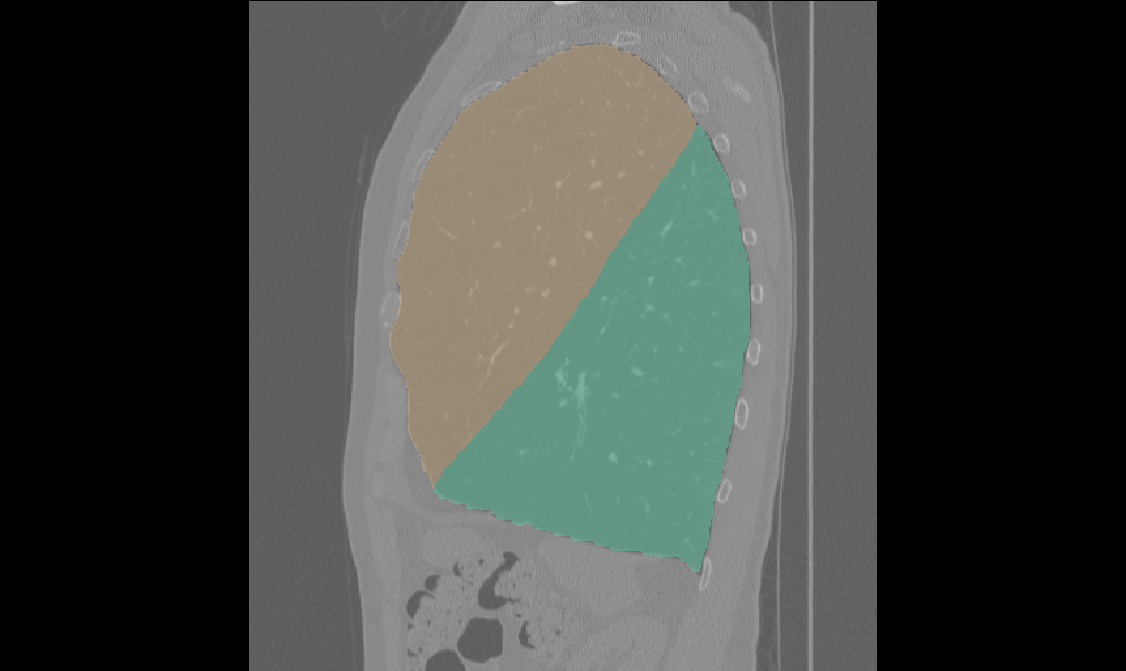
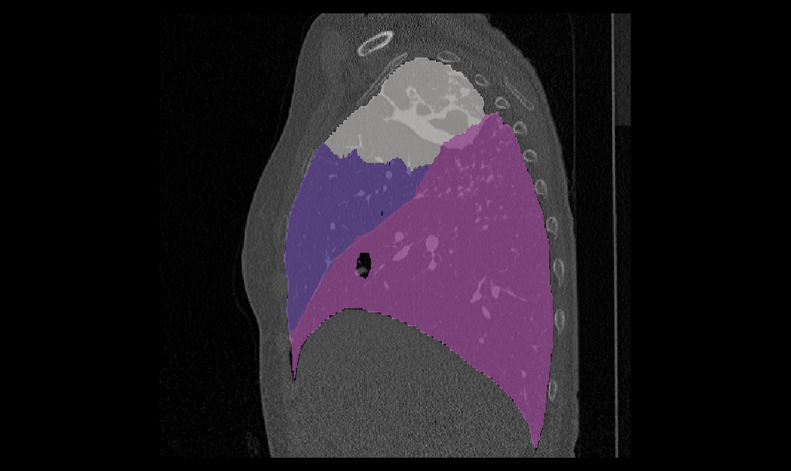
(a) (b) (c) (d)

Figure 7: (a) Input image. Outputs of : (b) Segmentation. (c) Input image. (d) Segmentation. Sagittal plane visualization of LOLA11 segmentation by our 3D PDV-Net: good cases (upper row) and failure cases (bottom row).

Figure 7 shows the segmentation results for the LOLA11 cases. For the left lung in Case 8, the LUL and LLL Dice scores were 0.9940 and 0.9926, respectively. For the right lung in Case 6, the scores are as follows: RUL: 0.9580, RML: 0.9480, and RLL: 0.9869. Again, for the left lung of Case 21, the segmentation Dice scores were relatively low. For the left lung in Case 21, the LUL score was 0.8170 and the LLL score was 0.3035. For the right lung in Case 55, although the right lower lobe was segmented with a high Dice score of 0.9818, because of the invisibility of the horizontal fissure, the RUL and RML had low segmentation Dice scores of 0.6827 and 0.7499, respectively.

4 Robustness Analysis

We further investigated the robustness of our model by grouping the 84 LIDC cases in three ways. For the first grouping, the Dice scores were put in three different Z-spacing buckets: $\hbox{Z-spacing}\leq 1$, $1<\hbox{Z-spacing}<2$, and $\hbox{Z-spacing}\geq 2$. In the second grouping, the Dice scores were put in four manufacturer buckets: GE, Philips, Siemens, and Toshiba. In the third grouping, the Dice scores were grouped according to the reconstruction kernel into 3 buckets: soft, lung, and bone. A one-way ANOVA analysis confirmed that there were no significant differences ($p\hbox{-value}<0.05$) between the average Dice scores of the buckets within each grouping, suggesting that our model is robust against the choice of reconstruction kernel, size of reconstruction interval, and different CT scanner vendors. Moreover, nodule volume in each of the 84 cases does not affect the lobe segmentation performance. There is no correlation between nodule volume and lobe segmentation accuracy, as indicated by the Pearson correlation ($p\hbox{-value}<0.05$).

We also studied how the segmentation correlation is affected by lung pathologies, by analyzing the correlation between Dice scores and the emphysema index; i.e., the proportion of the lungs affected by emphysema (in the range 0–1). For the LTRC cases, we associated lobe-wise emphysema indices by calculating the proportion of emphysema voxels (voxels marked as emphysema in the LTRC ground truth) in each of the lobes, as well as overall emphysema indices for both lungs. Figure 8 shows plots of the per-lobe and overall emphysema indexes versus segmentation performance. The small Pearson correlation ($p\hbox{-value}<0.05$) reveals that the lobe segmentation accuracy is uncorrelated with the emphysema index, confirming the robustness of our model in segmenting lobes in pathological cases.

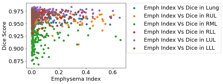
Figure 8: Plots of lobe-wise and overall segmentation accuracy (Dice scores) of our model versus the emphysema indices of the LTRC test cases reveal insignificant correlation.

5 Speed Analysis

Our 3D PDV-Net model takes approximately 2 seconds to segment lung lobes from one CT scan using a single Nvidia Titan XP GPU, which is six times faster than the 2D U-Net model. To our knowledge from the lung lobe segmentation models reported in literature, ours is by far the fastest model. Note that no prior published research considered a 3D convolutional model for lung lobe segmentation.

Appendix 7.G Conclusions

Reliable and automatic lung lobe segmentation is a challenging task, especially in the presence of pathologies and incomplete fissures. We introduced a new 3D CNN-based segmentation technique, namely, Progressive Dense V-Networks (PDV-Nets), and applied it to the automatic, fast, and reliable segmentation of lung lobes from chest CT scans. We evaluated our method using three test datasets—84 cases from LIDC, 154 cases from LTRC, and 55 cases from LOLA11. Our results demonstrated that our model outperforms, or at worst performs comparably to, the state-of-the-art while running at an average speed of 2 seconds per case, without requiring any prior segmentation. Furthermore, we demonstrated the robustness of our method against varying configurations of CT reconstruction, choice of CT imaging device vendor, and the presence of lung pathologies.

References

- Abadi et al. [2016] Abadi, M., Barham, P., Chen, J., Chen, Z., Davis, A., Dean, J., Devin, M., Ghemawat, S., Irving, G., Isard, M., et al. (2016). TensorFlow: A system for large-scale machine learning. In Proceedings of the USENIX Symposium on Operating Systems Design and Implementation (OSDI), pages 265–283.
- Acuna et al. [2019] Acuna, D., Kar, A., and Fidler, S. (2019). Devil is in the edges: Learning semantic boundaries from noisy annotations. In Proceedings of the IEEE Conference on Computer Vision and Pattern Recognition (CVPR).
- Armato et al. [2011] Armato, S. G., McLennan, G., Bidaut, L., McNitt-Gray, M. F., Meyer, C. R., Reeves, A. P., Zhao, B., Aberle, D. R., Henschke, C. I., Hoffman, E. A., et al. (2011). The lung image database consortium (LIDC) and image database resource initiative (IDRI): A completed reference database of lung nodules on CT scans. Medical Physics, 38(2):915–931.
- Audebert et al. [2016] Audebert, N., Le Saux, B., and Lefèvre, S. (2016). Semantic segmentation of earth observation data using multimodal and multi-scale deep networks. In Proceedings of the Asian Conference on Computer Vision (ACCV), pages 180–196. Springer.
- Aziz et al. [2004] Aziz, A., Ashizawa, K., Nagaoki, K., and Hayashi, K. (2004). High resolution CT anatomy of the pulmonary fissures. Journal of Thoracic Imaging, 19(3):186–191.
- Badrinarayanan et al. [2017] Badrinarayanan, V., Kendall, A., and Cipolla, R. (2017). Segnet: A deep convolutional encoder-decoder architecture for image segmentation. IEEE Transactions on Pattern Analysis and Machine Intelligence, 39(12):2481–2495.
- Baillard et al. [2000] Baillard, C., Barillot, C., and Bouthemy, P. (2000). Robust Adaptive Segmentation of 3D Medical Images with Level Sets. Research Report RR-4071, INRIA.
- Bakas et al. [2017] Bakas, S., Akbari, H., Sotiras, A., Bilello, M., Rozycki, M., Kirby, J., Freymann, J., Farahani, K., and Davatzikos, C. (2017). Advancing the cancer genome atlas glioma MRI collections with expert segmentation labels and radiomic features. Scientific Data, 4.
- Bauer et al. [2018] Bauer, C., Eberlein, M., and Beichel, R. (2018). Pulmonary lobe separation in expiration chest CT scans based on subject-specific priors derived from inspiration scans. Journal of Medical Imaging, 5(1):014003.
- Bischke et al. [2019] Bischke, B., Helber, P., Folz, J., Borth, D., and Dengel, A. (2019). Multi-task learning for segmentation of building footprints with deep neural networks. In Proceedings of the IEEE International Conference on Image Processing (ICIP), pages 1480–1484. IEEE.
- Blaffert et al. [2010] Blaffert, T., Wiemker, R., Barschdorf, H., Kabus, S., Klinder, T., Lorenz, C., Schadewaldt, N., and Dharaiya, E. (2010). A completely automated processing pipeline for lung and lung lobe segmentation and its application to the LIDC-IDRI data base. In Proceedings of Medical Imaging 2010: Image Processing, volume 7623, page 762347. International Society for Optics and Photonics.
- Bragman et al. [2017] Bragman, F. J., McClelland, J. R., Jacob, J., Hurst, J. R., and Hawkes, D. J. (2017). Pulmonary lobe segmentation with probabilistic segmentation of the fissures and a groupwise fissure prior. IEEE Transactions on Medical Imaging, 36(8):1650–1663.
- Bray et al. [2018] Bray, F., Ferlay, J., Soerjomataram, I., Siegel, R. L., Torre, L. A., and Jemal, A. (2018). Global cancer statistics 2018: Globocan estimates of incidence and mortality worldwide for 36 cancers in 185 countries. CA: A Cancer Journal for Clinicians, 68(6):394–424.
- Bulatov [2018] Bulatov, Y. (2018). Saving memory using gradient-checkpointing. https://github.com/openai/gradient-checkpointing, 01/01/2018.
- Cao et al. [2019] Cao, Z., Zhang, T., Diao, W., Zhang, Y., Lyu, X., Fu, K., and Sun, X. (2019). Meta-Seg: A generalized meta-learning framework for multi-class few-shot semantic segmentation. IEEE Access, 7:166109–166121.
- Caselles et al. [1997] Caselles, V., Kimmel, R., and Sapiro, G. (1997). Geodesic active contours. International Journal of Computer Vision, 22(1):61–79.
- Chan and Vese [2001] Chan, T. F. and Vese, L. A. (2001). Active contours without edges. IEEE Transactions on Image Processing, 10(2):266–277.
- Chen et al. [2016] Chen, H., Qi, X., Yu, L., and Heng, P.-A. (2016). DCAN: Deep contour-aware networks for accurate gland segmentation. In Proceedings of the IEEE Conference on Computer Vision and Pattern Recognition (CVPR), pages 2487–2496.
- Chen et al. [2014] Chen, L.-C., Papandreou, G., Kokkinos, I., Murphy, K., and Yuille, A. L. (2014). Semantic image segmentation with deep convolutional nets and fully connected CRFs. arXiv preprint arXiv:1412.7062.
- Chen et al. [2017a] Chen, L.-C., Papandreou, G., Kokkinos, I., Murphy, K., and Yuille, A. L. (2017a). Deeplab: Semantic image segmentation with deep convolutional nets, atrous convolution, and fully connected CRFs. IEEE Transactions on Pattern Analysis and Machine Intelligence, 40(4):834–848.
- Chen et al. [2017b] Chen, L.-C., Papandreou, G., Schroff, F., and Adam, H. (2017b). Rethinking atrous convolution for semantic image segmentation. arXiv preprint arXiv:1706.05587.
- Chen et al. [2018] Chen, L.-C., Zhu, Y., Papandreou, G., Schroff, F., and Adam, H. (2018). Encoder-decoder with atrous separable convolution for semantic image segmentation. In Proceedings of the European Conference on Computer Vision (ECCV), pages 801–818.
- Chen et al. [2019a] Chen, X., Qi, D., and Shen, J. (2019a). Boundary-aware network for fast and high-accuracy portrait segmentation. arXiv preprint arXiv:1901.03814.
- Chen et al. [2019b] Chen, X., Williams, B. M., Vallabhaneni, S. R., Czanner, G., Williams, R., and Zheng, Y. (2019b). Learning active contour models for medical image segmentation. In Proceedings of the IEEE Conference on Computer Vision and Pattern Recognition (CVPR), pages 11632–11640.
- Cheng et al. [2019] Cheng, D., Liao, R., Fidler, S., and Urtasun, R. (2019). DARNet: Deep active ray network for building segmentation. In Proceedings of the IEEE Conference on Computer Vision and Pattern Recognition (CVPR), pages 7431–7439.
- Çiçek et al. [2016] Çiçek, Ö., Abdulkadir, A., Lienkamp, S. S., Brox, T., and Ronneberger, O. (2016). 3D U-Net: learning dense volumetric segmentation from sparse annotation. In Proceedings of the International Conference on Medical Image Computing and Computer-Assisted Intervention (MICCAI), pages 424–432. Springer.
- Cordts et al. [2016] Cordts, M., Omran, M., Ramos, S., Rehfeld, T., Enzweiler, M., Benenson, R., Franke, U., Roth, S., and Schiele, B. (2016). The cityscapes dataset for semantic urban scene understanding. In Proceedings of the IEEE Conference on Computer Vision and Pattern Recognition (CVPR), pages 3213–3223.
- Deudon [2018] Deudon, M. (2018). Learning semantic similarity in a continuous space. In Advances in Neural Information Processing Systems, pages 986–997.
- Doel et al. [2012] Doel, T., Matin, T., Gleeson, F., Gavaghan, D., and Grau, V. (2012). Pulmonary lobe segmentation from CT images using fissureness, airways, vessels, and multilevel B-splines. Proceedings of the IEEE International Symposium on Biomedical Imaging (ISBI), 9:1491–1494.
- Dong and Xing [2018] Dong, N. and Xing, E. (2018). Few-shot semantic segmentation with prototype learning. In Proceedings of the British Machine Vision Conference (BMVC), volume 3.
- Dong et al. [2019] Dong, Z., Zhang, R., Shao, X., and Zhou, H. (2019). Multi-scale discriminative location-aware network for few-shot semantic segmentation. In Proceedings of the IEEE Annual Computer Software and Applications Conference (COMPSAC), volume 2, pages 42–47.
- Everingham et al. [2015] Everingham, M., Eslami, S. M. A., Van Gool, L., Williams, C. K. I., Winn, J., and Zisserman, A. (2015). The pascal visual object classes challenge: A retrospective. International Journal of Computer Vision, 111(1):98–136.
- Ferreira et al. [2018] Ferreira, F. T., Sousa, P., Galdran, A., Sousa, M. R., and Campilho, A. (2018). End-to-end supervised lung lobe segmentation. In Proceedings of the International Joint Conference on Neural Networks (IJCNN), pages 1–8. IEEE.
- Garcia and Bruna [2017] Garcia, V. and Bruna, J. (2017). Few-shot learning with graph neural networks. arXiv preprint arXiv:1711.04043.
- Geirhos et al. [2019] Geirhos, R., Rubisch, P., Michaelis, C., Bethge, M., Wichmann, F. A., and Brendel, W. (2019). ImageNet-trained CNNs are biased towards texture: Increasing shape bias improves accuracy and robustness. In Proceedings of the International Conference on Learning Representations (ICLR).
- George et al. [2017] George, K., Harrison, A., Jin, D., Xu, Z., and Mollura, D. (2017). Pathological pulmonary lobe segmentation from CT images using progressive holistically nested neural networks and random walker. DLMIA Lecture Notes in Computer Science, page 10553.
- Gibson et al. [2018a] Gibson, E., Giganti, F., Hu, Y., Bonmati, E., Bandula, S., Gurusamy, K., Davidson, B., Pereira, S. P., Clarkson, M. J., and Barratt, D. C. (2018a). Automatic multi-organ segmentation on abdominal CT with dense V-networks. IEEE Transactions on Medical Imaging, 37(8):1822–1834.
- Gibson et al. [2018b] Gibson, E., Giganti, F., Hu, Y., Bonmati, E., Bandula, S., Gurusamy, K., Davidson, B., Pereira, S. P., Clarkson, M. J., and Barratt, D. C. (2018b). Automatic multi-organ segmentation on abdominal CT with dense v-networks. IEEE Transactions on Medical Imaging.
- Giuliani et al. [2018] Giuliani, N., Payer, C., Pienn, M., Olschewski, H., and Urschler, M. (2018). Pulmonary lobe segmentation in CT image using alpha-expansion. Proceedings of VISIGRAPP, pages 387–394.
- Gulsun et al. [2006] Gulsun, M., Ariyurek, O., Comert, R., and Karabulut, N. (2006). Variability of the pulmonary oblique fissures presented by high-resolution computed tomography. Surgical Radilogic Anatomy, 28(3):293–299.
- Gur et al. [2019a] Gur, S., Shaharabany, T., and Wolf, L. (2019a). End to end trainable active contours via differentiable rendering. In Proceedings of the International Conference on Learning Representations (ICLR).
- Gur et al. [2019b] Gur, S., Wolf, L., Golgher, L., and Blinder, P. (2019b). Unsupervised microvascular image segmentation using an active contours mimicking neural network. In Proceedings of the IEEE International Conference on Computer Vision (ICCV), pages 10722–10731.
- Harrison et al. [2017] Harrison, A. P., Xu, Z., George, K., Lu, L., Summers, R. M., and Mollura, D. J. (2017). Progressive and multi-path holistically nested neural networks for pathological lung segmentation from CT images. In Proceedings of the International Conference on Medical Image Computing and Computer-Assisted Intervention (MICCAI), pages 621–629.
- Hatamizadeh [2020] Hatamizadeh, A. (2020). An Artificial Intelligence Framework for the Automated Segmentation and Quantitative Analysis of Retinal Vasculature. PhD thesis, UCLA.
- Hatamizadeh et al. [2019a] Hatamizadeh, A., Hoogi, A., Sengupta, D., Lu, W., Wilcox, B., Rubin, D., and Terzopoulos, D. (2019a). Deep active lesion segmentation. In Proceedings of the International Workshop on Machine Learning in Medical Imaging, pages 98–105. Springer.
- Hatamizadeh et al. [2019b] Hatamizadeh, A., Hosseini, H., Liu, Z., Schwartz, S. D., and Terzopoulos, D. (2019b). Deep dilated convolutional nets for the automatic segmentation of retinal vessels. In Proceedings of the International Conference on Machine Learning and Data Mining (MLDM), pages 39–48.
- Hatamizadeh et al. [2019c] Hatamizadeh, A., Sengupta, D., and Terzopoulos, D. (2019c). End-to-end deep convolutional active contours for image segmentation. arXiv preprint arXiv:1909.13359.
- Hatamizadeh et al. [2019d] Hatamizadeh, A., Terzopoulos, D., and Myronenko, A. (2019d). Boundary aware networks for medical image segmentation. arXiv preprint arXiv:1908.08071.
- Hatamizadeh et al. [2019e] Hatamizadeh, A., Terzopoulos, D., and Myronenko, A. (2019e). End-to-end boundary aware networks for medical image segmentation. In Proceedings of the International Workshop on Machine Learning in Medical Imaging (MLMI), pages 187–194. Springer.
- Hatamizadeh et al. [2020] Hatamizadeh, A., Terzopoulos, D., and Myronenko, A. (2020). Edge-gated CNNs for volumetric semantic segmentation of medical images. arXiv preprint arXiv:2002.04207.
- He et al. [2017] He, K., Gkioxari, G., Dollár, P., and Girshick, R. (2017). Mask R-CNN. In Proceedings of the IEEE International Conference on Computer Vision (ICCV), pages 2980–2988. IEEE.
- He et al. [2016] He, K., Zhang, X., Ren, S., and Sun, J. (2016). Deep residual learning for image recognition. In Proceedings of the IEEE Conference on Computer Vision and Pattern Recognition (CVPR), pages 770–778.
- Heller et al. [2019] Heller, N., Sathianathen, N., Kalapara, A., Walczak, E., Moore, K., Kaluzniak, H., Rosenberg, J., Blake, P., Rengel, Z., Oestreich, M., et al. (2019). The KiTS19 challenge data: 300 kidney tumor cases with clinical context, CT semantic segmentations, and surgical outcomes. arXiv preprint arXiv:1904.00445.
- Hoogi et al. [2017] Hoogi, A., Subramaniam, A., Veerapaneni, R., and Rubin, D. L. (2017). Adaptive estimation of active contour parameters using convolutional neural networks and texture analysis. IEEE Transactions on Medical Imaging, 36(3):781–791.
- Hu et al. [2017] Hu, P., Shuai, B., Liu, J., and Wang, G. (2017). Deep level sets for salient object detection. In Proceedings of the IEEE Conference on Computer Vision and Pattern Recognition (CVPR).
- Hu et al. [2019a] Hu, T., Yang, P., Zhang, C., Yu, G., Mu, Y., and Snoek, C. G. M. (2019a). Attention-based multi-context guiding for few-shot semantic segmentation. In Proceedings of the AAAI Conference on Artificial Intelligence.
- Hu et al. [2019b] Hu, Y., Zou, Y., and Feng, J. (2019b). Panoptic edge detection. https://arxiv.org/abs/1906.00590.
- Imran et al. [2019] Imran, A.-A.-Z., Hatamizadeh, A., Ananth, S. P., Ding, X., Tajbakhsh, N., and Terzopoulos, D. (2019). Fast and automatic segmentation of pulmonary lobes from chest CT using a progressive dense V-network. Computer Methods in Biomechanics and Biomedical Engineering: Imaging & Visualization, pages 1–10.
- Imran et al. [2018] Imran, A.-A.-Z., Hatamizadeh, A., Ananth, S. P., Ding, X., Terzopoulos, D., and Tajbakhsh, N. (2018). Automatic segmentation of pulmonary lobes using a progressive dense V-network. In Deep Learning in Medical Image Analysis, volume 11045 of Lecture Notes in Computer Science, pages 282–290. Springer.
- Ioffe and Szegedy [2015] Ioffe, S. and Szegedy, C. (2015). Batch normalization: Accelerating deep network training by reducing internal covariate shift. arXiv preprint arXiv:1502.03167.
- Iwano et al. [2013] Iwano, S., Kitano, M., Matsuo, K., Kawakami, K., Koike, W., Kishimoto, M., Inoue, T., Li, Y., and Naganawa, S. (2013). Pulmonary lobar volumetry using novel volumetric computer-aided diagnosis and computed tomography. Interactive Cardiovascular and Thoracic Surgery, 17(1):59–65.
- Jackson et al. [2018] Jackson, P., Hardcastle, N., Dawe, N., Kron, T., Hofman, M., and Hicks, R. J. (2018). Deep learning renal segmentation for fully automated radiation dose estimation in unsealed source therapy. Frontiers in oncology, 8:215.
- Jang et al. [2016] Jang, E., Gu, S., and Poole, B. (2016). Categorical reparameterization with gumbel-softmax. arXiv preprint arXiv:1611.01144.
- Jiang et al. [2018] Jiang, C., Qi, S., Zhu, Y., Huang, S., Lin, J., Yu, L., Terzopoulos, D., and Zhu, S. (2018). Configurable 3D scene synthesis and 2D image rendering with per-pixel ground truth using stochastic grammars. International Journal of Computer Vision, 126(9):920–941.
- Jin et al. [2019] Jin, Q., Meng, Z., Pham, T. D., Chen, Q., Wei, L., and Su, R. (2019). DUNet: A deformable network for retinal vessel segmentation. Knowledge-Based Systems, 178:149–162.
- Karwoski et al. [2008] Karwoski, R. A., Bartholmai, B., Zavaletta, V. A., Holmes, D., and Robb, R. A. (2008). Processing of CT images for analysis of diffuse lung disease in the lung tissue research consortium. In Proceedings of Medical Imaging 2008, volume 6916, page 691614. International Society for Optics and Photonics.
- Kass et al. [1988] Kass, M., Witkin, A., and Terzopoulos, D. (1988). Snakes: Active contour models. International Journal of Computer Vision, 1(4):321–331.
- Kim et al. [2019] Kim, J., Oh, T.-H., Lee, S., Pan, F., and Kweon, I. S. (2019). Variational prototyping-encoder: One-shot learning with prototypical images. In Proceedings of the IEEE Conference on Computer Vision and Pattern Recognition (CVPR), pages 9462–9470.
- Kingma and Ba [2014] Kingma, D. P. and Ba, J. (2014). Adam: A method for stochastic optimization. arXiv:1412.6980.
- Kingma and Welling [2013] Kingma, D. P. and Welling, M. (2013). Auto-encoding variational bayes. arXiv preprint arXiv:1312.6114.
- Koch et al. [2015] Koch, G., Zemel, R., and Salakhutdinov, R. (2015). Siamese neural networks for one-shot image recognition. In Proceedings of the ICML Deep Learning Workshop, volume 2. Lille.
- Lake et al. [2015] Lake, B. M., Salakhutdinov, R., and Tenenbaum, J. B. (2015). Human-level concept learning through probabilistic program induction. Science, 350(6266):1332–1338.
- Lankton and Tannenbaum [2008] Lankton, S. and Tannenbaum, A. (2008). Localizing region-based active contours. IEEE Transactions on Image Processing, 17(11):2029–2039.
- Lassen and van Rikxoort [2013] Lassen, B. and van Rikxoort, E. (2013). Automatic segmentation of the pulmonary lobes from chest CT scans based on fissures, vessels, and bronchi. IEEE Transactions on Medical Imaging, 32(2):210–222.
- Lassen-Schmidt et al. [2017] Lassen-Schmidt, B., Kuhnigk, J., Konrad, O., Van Ginneken, B., and Van Rikxoort, E. (2017). Fast interactive segmentation of the pulmonary lobes from thoracic computed tomography data. Physics in Medicine and Biology, 62(16):6649.
- Le et al. [2018] Le, T. H. N., Quach, K. G., Luu, K., Duong, C. N., and Savvides, M. (2018). Reformulating level sets as deep recurrent neural network approach to semantic segmentation. IEEE Transactions on Image Processing, 27(5):2393–2407.
- Li et al. [2018] Li, X., Chen, H., Qi, X., Dou, Q., Fu, C.-W., and Heng, P.-A. (2018). H-DenseUNet: hybrid densely connected unet for liver and tumor segmentation from CT volumes. IEEE Transactions on Medical Imaging, 37(12):2663–2674.
- Lifchitz et al. [2019] Lifchitz, Y., Avrithis, Y., Picard, S., and Bursuc, A. (2019). Dense classification and implanting for few-shot learning. In Proceedings of the IEEE Conference on Computer Vision and Pattern Recognition (CVPR), pages 9258–9267.
- Lim et al. [2016] Lim, H.-j., Weinheimer, O., Wielpütz, M. O., Dinkel, J., Hielscher, T., Gompelmann, D., Kauczor, H.-U., and Heussel, C. P. (2016). Fully automated pulmonary lobar segmentation: Influence of different prototype software programs onto quantitative evaluation of chronic obstructive lung disease. PLoS One, 11(3):e0151498.
- Liu et al. [2015] Liu, W., Rabinovich, A., and Berg, A. C. (2015). Parsenet: Looking wider to see better. arXiv preprint arXiv:1506.04579.
- LOLA11 [2011] LOLA11 (2011). Lobe and lung analysis. http://lola11.com.
- Long et al. [2015] Long, J., Shelhamer, E., and Darrell, T. (2015). Fully convolutional networks for semantic segmentation. In Proceedings of the IEEE Conference on Computer Vision and Pattern Recognition (CVPR), pages 3431–3440.
- Marcos et al. [2018] Marcos, D., Tuia, D., Kellenberger, B., Zhang, L., Bai, M., Liao, R., and Urtasun, R. (2018). Learning deep structured active contours end-to-end. In Proceedings of the IEEE Conference on Computer Vision and Pattern Recognition (CVPR), pages 8877–8885.
- Marquez-Neila et al. [2013] Marquez-Neila, P., Baumela, L., and Alvarez, L. (2013). A morphological approach to curvature-based evolution of curves and surfaces. IEEE Transactions on Pattern Analysis and Machine Intelligence, 36(1):2–17.
- McInerney et al. [2002] McInerney, T., Hamarneh, G., Shenton, M., and Terzopoulos, D. (2002). Deformable organisms for automatic medical image analysis. Medical Image Analysis, 6(3):251–266.
- McInerney and Terzopoulos [1996] McInerney, T. and Terzopoulos, D. (1996). Deformable models in medical image analysis: A survey. Medical Image Analysis, 1(2):91–108.
- Milletari et al. [2016] Milletari, F., Navab, N., and Ahmadi, S. (2016). V-net: Fully convolutional neural networks for volumetric medical image segmentation. In Proceedings of the International Conference on 3D Vision (3DV), pages 565–571. IEEE.
- Minaee et al. [2020] Minaee, S., Boykov, Y., Porikli, F., Plaza, A., Kehtarnavaz, N., and Terzopoulos, D. (2020). Image segmentation using deep learning: A survey. arXiv preprint arXiv:2001.05566.
- Murugesan et al. [2019] Murugesan, B., Sarveswaran, K., Shankaranarayana, S. M., Ram, K., Joseph, J., and Sivaprakasam, M. (2019). Psi-Net: Shape and boundary aware joint multi-task deep network for medical image segmentation. In Proceedings of the International Conference of the IEEE Engineering in Medicine and Biology Society (EMBC), pages 7223–7226. IEEE.
- Myronenko [2018] Myronenko, A. (2018). 3D MRI brain tumor segmentation using autoencoder regularization. In BrainLes, Medical Image Computing and Computer Assisted Intervention (MICCAI), Lecture Notes in Computer Science, pages 311–320. Springer.
- Myronenko and Hatamizadeh [2019a] Myronenko, A. and Hatamizadeh, A. (2019a). 3D kidneys and kidney tumor semantic segmentation using boundary-aware networks. Kidney Tumor Segmentation Challenge.
- Myronenko and Hatamizadeh [2019b] Myronenko, A. and Hatamizadeh, A. (2019b). Robust semantic segmentation of brain tumor regions from 3D MRIs. In Proceedings of the International MICCAI Brainlesion Workshop, pages 82–89. Springer.
- Ngo et al. [2017] Ngo, T. A., Lu, Z., and Carneiro, G. (2017). Combining deep learning and level set for the automated segmentation of the left ventricle of the heart from cardiac cine magnetic resonance. Medical Image Analysis, 35:159–171.
- Nguyen and Todorovic [2019] Nguyen, K. and Todorovic, S. (2019). Feature weighting and boosting for few-shot segmentation. In Proceedings of the IEEE International Conference on Computer Vision (ICCV), pages 622–631.
- Noh et al. [2015] Noh, H., Hong, S., and Han, B. (2015). Learning deconvolution network for semantic segmentation. In Proceedings of the IEEE International Conference on Computer Vision (ICCV), pages 1520–1528.
- Oliveira et al. [2009] Oliveira, D. A. B., Feitosa, R. Q., and Correia, M. M. (2009). Liver segmentation using level sets and genetic algorithms. In Proceedings of VISAPP (2), pages 154–159.
- Osher and Fedkiw [2001] Osher, S. and Fedkiw, R. P. (2001). Level set methods: An overview and some recent results. Journal of Computational Physics, 169(2):463–502.
- Osher and Sethian [1988] Osher, S. and Sethian, J. A. (1988). Fronts propagating with curvature-dependent speed: algorithms based on Hamilton-Jacobi formulations. Journal of Computational Physics, 79(1):12–49.
- Pu et al. [2009] Pu, J., Zheng, B., Leader, J., Fuhrman, C., Knollmann, F., Klym, A., and Gur, D. (2009). Pulmonary lobe segmentation in CT examinations using implicit surface fitting. IEEE Transactions on Medical Imaging, 28(12):1986–1996.
- Raasch et al. [1982] Raasch, B., Carsky, E., Lane, E., O’Callaghan, J., and Heitzman, E. (1982). Radiographic anatomy of the interlobar fissures: A study of 100 specimens. American Journal of Roentgenology, 138(6):1043–1049.
- Rakelly et al. [2018] Rakelly, K., Shelhamer, E., Darrell, T., Efros, A., and Levine, S. (2018). Conditional networks for few-shot semantic segmentation. In Proceedings of the International Conference on Learning Representations Workshop.
- Ronneberger et al. [2015] Ronneberger, O., Fischer, P., and Brox, T. (2015). U-Net: Convolutional networks for biomedical image segmentation. In Proceedings of the International Conference on Medical Image Computing and Computer-Assisted Intervention (MICCAI), volume 9351 of Lecture Notes in Computer Science, pages 234–241. Springer.
- Rosenfeld [1976] Rosenfeld, A. (1976). Digital Picture Processing. Academic Press.
- Ross et al. [2010] Ross, J., Estépar, R. S. J., Kindlmann, G., Díaz, A., Westin, C., Silverman, E., and Washko, G. (2010). Automatic lobe segmentation using particles, thin plate splines, and a maximum a posteriori estimation. In Proceedings of the International Conference on Medical Image Computing and Computer Assisted Intervention (MICCAI), volume 6363, pages 163–171.
- Rudner et al. [2019] Rudner, T. G., Rußwurm, M., Fil, J., Pelich, R., Bischke, B., Kopačková, V., and Biliński, P. (2019). Multi3Net: segmenting flooded buildings via fusion of multiresolution, multisensor, and multitemporal satellite imagery. In Proceedings of the AAAI Conference on Artificial Intelligence, volume 33, pages 702–709.
- Russakovsky et al. [2015] Russakovsky, O., Deng, J., Su, H., Krause, J., Satheesh, S., Ma, S., Huang, Z., Karpathy, A., Khosla, A., Bernstein, M., et al. (2015). Imagenet large scale visual recognition challenge. International Journal of Computer Vision, 115(3):211–252.
- Schonfeld et al. [2019] Schonfeld, E., Ebrahimi, S., Sinha, S., Darrell, T., and Akata, Z. (2019). Generalized zero-and few-shot learning via aligned variational autoencoders. In Proceedings of the IEEE Conference on Computer Vision and Pattern Recognition (CVPR), pages 8247–8255.
- Shaban et al. [2017] Shaban, A., Bansal, S., Liu, Z., Essa, I., and Boots, B. (2017). One-shot learning for semantic segmentation. arXiv preprint arXiv:1709.03410.
- Shen et al. [2017] Shen, H., Wang, R., Zhang, J., and McKenna, S. J. (2017). Boundary-aware fully convolutional network for brain tumor segmentation. In Proceedings of the International Conference on Medical Image Computing and Computer-Assisted Intervention (MICCAI), pages 433–441. Springer.
- Siam et al. [2019] Siam, M., Oreshkin, B., and Jagersand, M. (2019). Amp: Adaptive masked proxies for few-shot segmentation. In Proceedings of the IEEE International Conference on Computer Vision (ICCV), pages 5248–5257.
- Siegel et al. [2019] Siegel, R. L., Miller, K. D., and Jemal, A. (2019). Cancer statistics, 2019. CA: A Cancer Journal for Clinicians, 69(1):7–34.
- Silberman et al. [2014] Silberman, N., Sontag, D., and Fergus, R. (2014). Instance segmentation of indoor scenes using a coverage loss. In Proceedings of the European Conference on Computer Vision (ECCV), pages 616–631. Springer.
- Simonyan and Zisserman [2014] Simonyan, K. and Zisserman, A. (2014). Very deep convolutional networks for large-scale image recognition. arXiv preprint arXiv:1409.1556.
- Snell et al. [2017] Snell, J., Swersky, K., and Zemel, R. (2017). Prototypical networks for few-shot learning. In Advances in Neural Information Processing Systems, pages 4077–4087.
- Sonka et al. [2014] Sonka, M., Hlavac, V., and Boyle, R. (2014). Image Processing, Analysis, and Machine Vision, Fourth Edition. Cengage Learning.
- Sun et al. [2012] Sun, M., Abdollah, F., Bianchi, M., Trinh, Q.-D., Jeldres, C., Thuret, R., Tian, Z., Shariat, S. F., Montorsi, F., Perrotte, P., et al. (2012). Treatment management of small renal masses in the 21st century: a paradigm shift. Annals of surgical oncology, 19(7):2380–2387.
- Sung et al. [2018] Sung, F., Yang, Y., Zhang, L., Xiang, T., Torr, P. H., and Hospedales, T. M. (2018). Learning to compare: Relation network for few-shot learning. In Proceedings of the IEEE Conference on Computer Vision and Pattern Recognition (CVPR), pages 1199–1208.
- Takikawa et al. [2019] Takikawa, T., Acuna, D., Jampani, V., and Fidler, S. (2019). Gated-SCNN: Gated shape CNNs for semantic segmentation. In Proceedings of the IEEE International Conference on Computer Vision (ICCV), pages 5229–5238.
- Thong et al. [2018] Thong, W., Kadoury, S., Piché, N., and Pal, C. J. (2018). Convolutional networks for kidney segmentation in contrast-enhanced CT scans. Computer Methods in Biomechanics and Biomedical Engineering: Imaging & Visualization, 6(3):277–282.
- van Rikxoort et al. [2010] van Rikxoort, E., Prokop, M., de Hoop, B., Viergever, M., Pluim, J., and van Ginneken, B. (2010). Automatic segmentation of pulmonary lobes robust against incomplete fissures. IEEE Transactions on Medical Imaging, 29(6):1286–1296.
- Vinyals et al. [2016] Vinyals, O., Blundell, C., Lillicrap, T., Wierstra, D., et al. (2016). Matching networks for one shot learning. In Advances in Neural Information Processing Systems, pages 3630–3638.
- Wang et al. [2019] Wang, K., Liew, J. H., Zou, Y., Zhou, D., and Feng, J. (2019). PANet: Few-shot image semantic segmentation with prototype alignment. In Proceedings of the IEEE International Conference on Computer Vision (ICCV), pages 9197–9206.
- Wang et al. [2017] Wang, S., Bai, M., Mattyus, G., Chu, H., Luo, W., Yang, B., Liang, J., Cheverie, J., Fidler, S., and Urtasun, R. (2017). TorontoCity: Seeing the world with a million eyes. In Proceedings of the IEEE International Conference on Computer Vision (ICCV), pages 3009–3017.
- Wang et al. [2018] Wang, X., Teng, P., Lo, P., Banola, A., Kim, G., Abtin, F., Goldin, J., and Brown, M. (2018). High throughput lung and lobar segmentation by 2D and 3D CNN on chest CT with diffuse lung disease. In Image Analysis for Moving Organ, Breast, and Thoracic Images, pages 202–214. Springer.
- Wu et al. [2018] Wu, G., Shao, X., Guo, Z., Chen, Q., Yuan, W., Shi, X., Xu, Y., and Shibasaki, R. (2018). Automatic building segmentation of aerial imagery using multi-constraint fully convolutional networks. Remote Sensing, 10(3):407.
- Xia et al. [2019] Xia, K.-J., Yin, H.-S., and Zhang, Y.-D. (2019). Deep semantic segmentation of kidney and space-occupying lesion area based on scnn and resnet models combined with sift-flow algorithm. Journal of medical systems, 43(1):2.
- Xu et al. [2018] Xu, Y., Wu, L., Xie, Z., and Chen, Z. (2018). Building extraction in very high resolution remote sensing imagery using deep learning and guided filters. Remote Sensing, 10(1):144.
- Yang et al. [2018] Yang, G., Li, G., Pan, T., Kong, Y., Wu, J., Shu, H., Luo, L., Dillenseger, J.-L., Coatrieux, J.-L., Tang, L., et al. (2018). Automatic segmentation of kidney and renal tumor in CT images based on 3D fully convolutional neural network with pyramid pooling module. In Proceedings of the International Conference on Pattern Recognition (ICPR), pages 3790–3795. IEEE.
- Yang et al. [2020] Yang, G., Niu, D., Zhang, C., and Zhao, X. (2020). Recognizing novel patterns via adversarial learning for one-shot semantic segmentation. Information Sciences, 518:225 – 237.
- Yin et al. [2019] Yin, K., Liu, C., Bardis, M., Martin, J., Liu, H., Ushinsky, A., Glavis-Bloom, J., Chantaduly, C., Chow, D. S., Houshyar, R., et al. (2019). Deep learning segmentation of kidneys with renal cell carcinoma. Journal of Clinical Oncology, 37(15_suppl):e16098–e16098.
- Yu and Koltun [2015] Yu, F. and Koltun, V. (2015). Multi-scale context aggregation by dilated convolutions. arXiv preprint arXiv:1511.07122.
- Yu et al. [2017a] Yu, Z., Feng, C., Liu, M., and Ramalingam, S. (2017a). Casenet: Deep category-aware semantic edge detection. In Proceedings of the IEEE Conference on Computer Vision and Pattern Recognition (CVPR).
- Yu et al. [2017b] Yu, Z., Feng, C., Liu, M.-Y., and Ramalingam, S. (2017b). Casenet: Deep category-aware semantic edge detection. In Proceedings of the IEEE Conference on Computer Vision and Pattern Recognition (CVPR), pages 5964–5973.
- Yu et al. [2018] Yu, Z., Liu, W., Zou, Y., Feng, C., Ramalingam, S., Vijaya Kumar, B. V. K., and Kautz, J. (2018). Simultaneous edge alignment and learning. In Proceedings of the European Conference on Computer Vision (ECCV).
- Zhang et al. [2018] Zhang, X., Wei, Y., Yang, Y., and Huang, T. (2018). SG-One: Similarity guidance network for one-shot semantic segmentation. arXiv preprint arXiv:1810.09091.
- Zhang et al. [2019] Zhang, Z., Fu, H., Dai, H., Shen, J., Pang, Y., and Shao, L. (2019). ET-Net: A generic edge-attention guidance network for medical image segmentation. In Proceedings of the International Conference on Medical Image Computing and Computer-Assisted Intervention (MICCAI), pages 442–450. Springer.
- Zhao et al. [2017] Zhao, H., Shi, J., Qi, X., Wang, X., and Jia, J. (2017). Pyramid scene parsing network. In Proceedings of the IEEE Conference on Computer Vision and Pattern Recognition (CVPR), pages 2881–2890.
- Zhou et al. [2019] Zhou, Y., Onder, O. F., Dou, Q., Tsougenis, E., Chen, H., and Heng, P.-A. (2019). CIA-Net: Robust nuclei instance segmentation with contour-aware information aggregation. In Proceedings of the International Conference on Information Processing in Medical Imaging (IPMI), pages 682–693. Springer.