Inexact Derivative-Free Optimization for Bilevel Learning

Abstract

Variational regularization techniques are dominant in the field of mathematical imaging. A drawback of these techniques is that they are dependent on a number of parameters which have to be set by the user. A by now common strategy to resolve this issue is to learn these parameters from data. While mathematically appealing this strategy leads to a nested optimization problem (known as bilevel optimization) which is computationally very difficult to handle. It is common when solving the upper-level problem to assume access to exact solutions of the lower-level problem, which is practically infeasible. In this work we propose to solve these problems using inexact derivative-free optimization algorithms which never require exact lower-level problem solutions, but instead assume access to approximate solutions with controllable accuracy, which is achievable in practice. We prove global convergence and a worst-case complexity bound for our approach. We test our proposed framework on ROF-denoising and learning MRI sampling patterns. Dynamically adjusting the lower-level accuracy yields learned parameters with similar reconstruction quality as high-accuracy evaluations but with dramatic reductions in computational work (up to 100 times faster in some cases).

1 Introduction

Variational regularization techniques are dominant in the field of mathematical imaging. For example, when solving a linear inverse problem $Ax=y$, variational regularization can be posed as the solution to

$$\min_{x}\mathcal{D}(Ax,y)+\alpha\mathcal{R}(x)\,.$$ (1)

Here the data fidelity $\mathcal{D}$ is usually chosen related to the assumed noise model of the data $y$ and the regularizer $\mathcal{R}$ models our a-priori knowledge of the unknown solution. Many options have been proposed in the literature, see for instance Ito2014book (1, 2, 3, 4, 5) and references therein. An important parameter for any variational regularization technique is the regularization parameter $\alpha$. While some theoretical results and heuristic choices have been proposed in there literature, see e.g. Engl1996 (6, 2) and references therein or the L-curve criterion Hansen1992lcurve (7), the appropriate choice of the regularization parameter in a practical setting remains an open problem. Similarly, other parameters in (1) have to be chosen by the user, such as smoothing of the total variation Chambolle2016actanumerica (3), the hyperparameter for total generalized variation Bredies2010 (8) or the sampling pattern in magnetic resonance imaging (MRI), see e.g. Usman2009 (9, 10, 11).

Instead of using heuristics for choosing all of these parameters, here we are interested in finding these from data. A by-now common strategy to learn parameters of a variational regularization model from data is bilevel learning, see e.g. DeLosReyes2013 (12, 13, 14, 15, 11, 16, 17) and references in Arridge2019 (4) . Given labelled data $(x_{i},y_{i})_{i=1,\ldots,n}$ we find parameters $\theta\in\Theta\subset\mathbb{R}^{m}$ by solving the upper-level problem

$$\min_{\theta\in\Theta}f(\theta):=\frac{1}{n}\sum_{i=1}^{n}\|\hat{x}_{i}(\theta)-x_{i}\|^{2}+\mathcal{J}(\theta),$$ (2)

where $\hat{x}_{i}(\theta)\in X\subset\mathbb{R}^{d}$ aims to recover the true data $x_{i}$ by solving the lower-level problems

$$\hat{x}_{i}(\theta):=\arg\min_{x\in X}\Phi_{i,\theta}(x),\qquad\forall i=1,\ldots,n\,.$$ (3)

The lower-level objective $\Phi_{i,\theta}$ could be of the form $\Phi_{i,\theta}(x)=\mathcal{D}(Ax,y_{i})+\theta\mathcal{R}(x)$ as in (1) but we will not restrict ourselves to this special case. In general $\Phi_{i,\theta}$ will depend on the data $y_{i}$.

In many situations, it is possible to acquire suitable data $(x_{i},y_{i})_{i=1,\ldots,n}$. For image denoising, we may take any ground truth images $x_{i}$ and add artificial noise to generate $y_{i}$. Alternatively, if we aim to learn a sampling pattern (such as for learning MRI sampling patterns, which we consider in this work), then $x_{i}$ can be any fully sampled image. The same also holds for problems such as image compression, where again $x_{i}$ is any ground truth image. In both these cases, $y_{i}$ is subsampled information from $x_{i}$ (depending on $\theta$) from which the remaining information is reconstructed to get $\hat{x}_{i}(\theta)$.

While mathematically appealing, this nested optimization problem is computationally very difficult to handle since even the evaluation of the upper-level problem (2) requires the exact solution of the lower-level problems (3). This requirement is practically infeasible and common algorithms in the literature compute the lower-level solution only to some accuracy, thereby losing any theoretical performance guarantees, see e.g. DeLosReyes2013 (12, 16, 11). One reason for needing exact solutions is to compute the gradient of the upper-level objective using the implicit function theorem Sherry2019sampling (11), which we address by using upper-level solvers which do not require gradient computations.

In this work we propose to solve these problems using inexact derivative-free optimization (DFO) algorithms which never require exact solutions to the lower-level problem while still yielding convergence guarantees. Moreover, by dynamically adjusting the accuracy we gain a significant computational speed-up compared to using a fixed accuracy for all lower-level solves. The proposed framework is tested on two problems: learning regularization parameters for ROF-denoising and learning the sampling pattern in MRI.

We contrast our approach to Kunisch2013bilevel (13), which develops a semismooth Newton method to solve the full bilevel optimality conditions. In Kunisch2013bilevel (13) the upper- and lower-level problems are of specific structure, and exact solutions of the (possibly very large) Newton system are required. Separately, the approach in Ochs2015 (14) replaces the lower-level problem with finitely many iterations of some algorithm and solves this perturbed problem exactly. Our formulation is very general and all approximations are controlled to guarantee convergence to the solution of the original variational problem.

Aim: Use inexact computations of $\hat{x}_{i}(\theta)$ within a derivative-free upper-level solver, which makes (2) computationally tractable, while retaining convergence guarantees.

1.1 Derivative-free optimization

Derivative-free optimization methods—that is, optimization methods that do not require access to the derivatives of the objective (and/or constraints)—have grown in popularity in recent years, and are particularly suited to settings where the objective is computationally expensive to evaluate and/or noisy; we refer the reader to Conn2009 (18, 19) for background on DFO and examples of applications, and to Larson2019 (20) for a comprehensive survey of recent work. The use of DFO for algorithm tuning has previously been considered in a general framework Audet2006a (21), and in the specific case of hyperparameter tuning for neural networks in Lakhmiri2019 (22).

Here, we are interested in the particular setting of learning for variational methods (2), which has also been considered in Riis2018 (16) where a new DFO algorithm based on discrete gradients has been proposed. In Riis2018 (16) it was assumed that the lower-level problem can be solved exactly such that the bilevel problem can be reduced to a single nonconvex optimization problem. In the present work we lift this stringent assumption.

In this paper we focus on DFO methods which are adapted to nonlinear least-squares problems as analyzed in Zhang2010 (23, 24). These methods are so-called ‘model-based’, in that they construct a model approximating the objective at each iteration, locally minimize the model to select the next iterate, and update the model with new objective information. Our work also connects to Conn2012 (25), which considers model-based bilevel optimization where both the lower- and upper-level problems are solved in a derivative-free manner; particular attention is given here to reusing evaluations of the (assumed expensive) lower-level objective at nearby upper-level parameters, to make lower-level model construction simpler.

Our approach for bilevel DFO is is based on dynamic-accuracy (derivative-based) trust-region methods (Conn2000, 26, Chapter 10.6). In these approaches, we use the measures of convergence (e.g. trust-region radius, model gradient) to determine a suitable level of accuracy with which to evaluate the objective; we start with low accuracy requirements, and increase the required accuracy as we converge to a solution. In a DFO context, this framework is the basis of Conn2012 (25), and a similar approach was considered in Chen2012 (27) in the context of analyzing protein structures. This framework has also been recently extended in a derivative-based context to higher-order regularization methods Bellavia2019 (28, 29). We also note that there has been some work on multilevel and multi-fidelity models (in both a DFO and derivative-based context), where an expensive objective can be approximated by surrogates which are cheaper to evaluate March2012 (30, 31).

1.2 Contributions

There are a number of novel aspects to this work. Our use of DFO for bilevel learning means our upper-level solver genuinely expects inexact lower-level solutions. We give worst-case complexity theory for our algorithm both in terms of upper-level iterations and computational work from the lower-level problems. Our numerical results on ROF-denoising and a new framework for learning MRI sampling patterns demonstrate our approach is substantially faster—up to 100 times faster—than the same DFO approach with high accuracy lower-level solutions, while achieving the same quality solutions. More details on the different aspects of our contributions are given below.

Dynamic accuracy DFO algorithm for bilevel learning

As noted in Sherry2019sampling (11), bilevel learning can require very high-accuracy solutions to the lower-level problem. We avoid this via the introduction of a dynamic accuracy model-based DFO algorithm. In this setting, the upper-level solver dynamically changes the required accuracy for lower-level problem minimizers, where less accuracy is required in earlier phases of the upper-level optimization. The proposed algorithm is similar to Conn2012 (25), but adapted to the nonlinear least-squares case and allowing derivative-based methods to solve the lower-level problem. Our theoretical results extend the convergence results of Conn2012 (25) to include derivative-based lower-level solvers and a least-squares structure, as well as adding a worst-case complexity analysis in a style similar to Cartis2019a (24) (which is also not present in the derivative-based convergence theory in Conn2000 (26)). This analysis gives bounds on the number of iterations of the upper-level solver required to reach a given optimality, which we then extend to bound the total computational effort required for the lower-level problem solves. There is increasing interest, but comparatively fewer works, which explicitly bound the total computational effort of nonconvex optimization methods; see Royer2020 (32) for Newton-CG methods and references therein. We provide a preliminary argument that our computational effort bounds are tight with regards to the desired upper-level solution accuracy, although we delegate a complete proof to future work.

Robustness

We observe in all our results using several lower-level solvers (gradient descent and FISTA) for a variety of applications that the proposed upper-level DFO algorithm converges to similar objective values and minimizers. We also present numerical results for denoising showing that the learned parameters are robust to initialization of the upper-level solver despite the upper-level problem being likely nonconvex. Together, these results suggest that this framework is a robust approach for bilevel learning.

Efficiency

Bilevel learning with a DFO algorithm was previously considered Riis2018 (16), but there a different DFO method based on discrete gradients was used, and was applied to nonsmooth problems with exact lower-level evaluations. In Riis2018 (16), only up to two parameters were learned, whereas here we demonstrate our approach is capable of learning many more. Our numerical results include examples with up to 64 parameters.

We demonstrate that the dynamic accuracy DFO achieves comparable or better objective values than the fixed accuracy variants and final reconstructions of comparable quality. However our approach is able to achieve this with a dramatically reduced computational load, in some cases up to 100 times less work than the fixed accuracy variants.

New framework for learning MRI sampling

We introduce a new framework to learn the sampling pattern in MRI based on bilevel learning. Our idea is inspired by the image inpainting model of Chen2014 (33). Compared to other algorithms to learn the sampling pattern in MRI based on first-order methods Sherry2019sampling (11), the proposed approach seems to be much more robust to initialization and choice of solver for the lower-level problem. As with the denoising examples, our dynamic accuracy DFO achieves the same upper-level objective values and final reconstructions as fixed accuracy variants but with substantial reductions in computational work.

Regularization parameter choice rule with machine learning

Our numerical results suggest that the bilevel framework can learn regularization parameter choice rule which yields a convergent regularization method in the sense of Scherzer2008book (5, 1), indicating for the first time that machine learning can be used to learn mathematically sound regularization methods.

1.3 Structure

In Section 2 we describe problems where the lower-level model (1) applies and describe how to efficiently attain a given accuracy level using standard first-order methods. Then in Section 3 we introduce the dynamic accuracy DFO algorithm and present our global convergence and worst-case complexity bounds. Finally, our numerical experiments are described in Section 4.

1.4 Notation

Throughout, we let $\|\cdot\|$ we denote the Euclidean norm of a vector in $\mathbb{R}^{n}$ and the operator 2-norm of a matrix in $\mathbb{R}^{m\times n}$. We also define the weighted (semi)norm $\|x\|^{2}_{S}:=x^{T}Sx$ for a symmetric and positive (semi)definite matrix $S$. The gradient of a scalar-valued function $f:\mathbb{R}^{n}\to\mathbb{R}$ is denoted by $\nabla f:\mathbb{R}^{n}\to\mathbb{R}^{n}$, and the derivative of a vector-valued function $f:\mathbb{R}^{n}\to\mathbb{R}^{m}$ is denoted by $\partial f:\mathbb{R}^{n}\to\mathbb{R}^{n\times m},(\partial f)_{i,j}=\partial_{i}f_{j}$ where $\partial_{i}f_{j}$ denotes the partial derivative of $f_{j}$ with respect to the $i$th coordinate. If $f$ is a function of two variables $x$ and $y$, then $\partial_{x}f$ denotes the derivative with respect to $x$.

1.5 Software

Our implementation of the DFO algorithm and all numerical testing code will be made public upon acceptance.

2 Lower-Level Problem

In order to have sufficient control over the accuracy of the solution to (3) we will assume that $\Phi_{i,\theta}$ are $L_{i}$-smooth and $\mu_{i}$-strongly convex, see definitions below.

Definition 1 (Smoothness)

A function $f:\mathbb{R}^{n}\to\mathbb{R}$ is $L$-smooth if it is differentiable and its derivative is Lipschitz continuous with constant $L>0$, i.e. for all $x,y\in\mathbb{R}^{n}$ we have $\|\nabla f(x)-\nabla f(y)\|\leq L\|x-y\|$.

Definition 2 (Strong Convexity)

A function $f:\mathbb{R}^{n}\to\mathbb{R}$ is $\mu$-strongly convex for $\mu>0$ if $f-\frac{\mu}{2}\|\cdot\|^{2}$ is convex.

Moreover, when the lower-level problem is strictly convex and smooth, with $\Phi_{i}(x,\theta):=\Phi_{i,\theta}(x)$ we can equivalently describe the minimizer of $\Phi_{i,\theta}$ by

$$\partial_{x}\Phi_{i}(\hat{x}_{i}(\theta),\theta)=0\,.$$ (4)

Smoothness properties of $\hat{x}_{i}$ follow from the implicit function theorem and its generalizations if $\Phi_{i}$ is smooth and regular enough.

Assumption 1

We assume that for all $i=1,\ldots,n$ the following statements hold.

1. Convexity: For all $\theta\in\Theta$ the functions $\Phi_{i,\theta}$ are $\mu_{i}$-strongly convex.

2. Smoothness in $x$: For all $\theta\in\Theta$ the functions $\Phi_{i,\theta}$ are $L_{i}$-smooth.

3. Smoothness in $(x,\theta)$: The derivatives $\partial_{x}\Phi_{i}:X\times\Theta\to X$ and $\partial_{xx}\Phi_{i}:X\times\Theta\to X^{2}$ exist and are continuous.

Theorem 2.1

Under Assumption 1 the function $\hat{x}_{i}(\theta):=\arg\min_{x}\Phi_{i}(x,\theta)$ is

1. well-defined

2. locally Lipschitz

3. continuously differentiable and
   $\partial\hat{x}_{i}(\theta)=-\partial_{xx}\Phi_{i}(\hat{x}_{i}(\theta),\theta)^{-1}\partial_{x}\partial_{\theta}\Phi_{i}(\hat{x}_{i}(\theta),\theta)$.

Proof

Ad 1) Finite and convex functions are continuous (Rockafellar2008, 34, Corollary 2.36). It is easy to show that $\mu$-strongly convex functions are coercive. Then the existence and uniqueness follows from classical theorems, e.g. (Bredies2018book, 35, Theorem 6.31). Ad 2) This statement follows directly from (Robinson1980, 36, Theorem 2.1). Ad 3) This follows directly from the classical inverse function theorem, see e.g. (Duistermaat2004a, 37, Theorem 3.5.1).

2.1 Examples

A relevant case of the model introduced above is the parameter tuning for linear inverse problems, which can be solved via the variational regularization model

$$\frac{1}{2}\|Ax-y_{i}\|^{2}_{S}+\alpha\operatorname{TV}(x),$$ (5)

where $\operatorname{TV}(x):=\sum_{j=1}^{m}\|\widehat{\nabla}x(j)\|$ denotes the discretized total variation, e.g. $\widehat{\nabla}x(j)$ is the finite forward difference discretization of the spatial gradient of $x$ at pixel $j$. However, we note that (5) does not satisfy Assumption 1.

To ensure Assumption 1 holds, we instead use $\|x\|\approx\sqrt{\|x\|^{2}+\nu^{2}}$, to approximate problem (5) by a smooth and strongly convex problem of the form

$$\hat{x}_{i}(\theta) :=\arg\min_{x}\left\{\Phi_{i,\theta}(x)=\frac{1}{2}\|A(\theta)x-y_{i}\|^{2}_{S(\theta)}\right.$$

$$\qquad\qquad\left.+\alpha(\theta)\operatorname{TV}_{\nu(\theta)}(x)+\frac{\xi(\theta)}{2}\|x\|^{2}\right\}\,,$$ (6)

with the smoothed total variation given by $\operatorname{TV}_{\nu(\theta)}(x):=\sum_{j=1}^{m}\sqrt{\|\widehat{\nabla}x(j)\|^{2}+\nu(\theta)^{2}}$. Here we already introduced the notation that various parts of the problem may depend on a vector of parameters $\theta$ which usually needs to be selected manually. We will learn these parameters using the bilevel framework. For simplicity denote $A_{\theta}:=A(\theta)$, $S_{\theta}:=S(\theta)$, $\alpha_{\theta}:=\alpha(\theta)$, $\nu_{\theta}:=\nu(\theta)$ and $\xi_{\theta}:=\xi(\theta)$. Note that $\Phi_{i,\theta}$ in (6) is $L_{i}$-smooth and $\mu_{i}$-strongly convex with

$$L_{i} \leq\|A_{\theta}^{*}S_{\theta}A_{\theta}\|+\alpha_{\theta}\frac{\|\partial\|^{2}}{\nu_{\theta}}+\xi_{\theta},\quad\text{and}$$

$$\mu_{i} \geq\lambda_{\operatorname{min}}(A_{\theta}^{*}S_{\theta}A_{\theta})+\xi_{\theta}\,,$$ (7)

where $\lambda_{\operatorname{min}}(A_{\theta}^{*}S_{\theta}A_{\theta})$ denotes the smallest eigenvalue of $A_{\theta}^{*}S_{\theta}A_{\theta}$ and $A_{\theta}^{*}$ is the adjoint of $A_{\theta}$.

We now describe two specific problems we will use in our numerical results. They both choose a specific form for (3) which aims to find a minimizer $\hat{x}_{i}(\theta)$ which (approximately) recovers the data $x_{i}$, and so both use (2) as the upper-level problem.

2.1.1 Total Variation-based Denoising

A particular problem we consider is a smoothed version of the ROF model Rudin1992ROF (38), i.e. $A_{\theta}=I,S_{\theta}=I$. Then (6) simplifies to

$$\Phi_{i,\theta}(x)=\frac{1}{2}\|x-y_{i}\|^{2}+\alpha_{\theta}\operatorname{TV}_{\nu_{\theta}}(x)+\frac{\xi_{\theta}}{2}\|x\|^{2},$$ (8)

which is $L_{i}$-smooth and $\mu_{i}$-strongly convex with constants as in (7) with $\|A_{\theta}^{*}S_{\theta}A_{\theta}\|=\|I\|=1$ and $\lambda_{\operatorname{min}}(A_{\theta}^{*}S_{\theta}A_{\theta})=\lambda_{\operatorname{min}}(I)=1$. In our numerical examples we will consider two cases. First, we will just learn the regularization parameter $\alpha$ given manually set $\nu$ and $\xi$. Second, we will learn all three parameters $\alpha,\nu$ and $\xi$.

2.1.2 Undersampled MRI Reconstruction

Another problem we consider is the reconstruction from undersampled MRI data, see e.g. Lustig2007sparseMRI (39), which can be phrased as (6) with $A_{\theta}=F$ where $F$ is the discrete Fourier transform and $S_{\theta}=\operatorname{diag}(s),s\in[0,1]^{d}$. Then (6) simplifies to

$$\Phi_{i,\theta}(x)=\frac{1}{2}\|Fx-y_{i}\|^{2}_{S_{\theta}}+\alpha_{\theta}\operatorname{TV}_{\nu_{\theta}}(x)+\frac{\xi_{\theta}}{2}\|x\|^{2},$$ (9)

which is $L_{i}$-smooth and $\mu_{i}$-strongly convex with constants as in (7) with $\|A_{\theta}^{*}S_{\theta}A_{\theta}\|\leq 1$ and $\lambda_{\operatorname{min}}(A_{\theta}^{*}S_{\theta}A_{\theta})\geq 0$. The sampling coefficients $s_{j}$ indicate the relevance of a sampling location. The data term (9) can be rewritten as

$$\|Fx-y_{i}\|^{2}_{S_{\theta}}=\sum_{s_{j}>0}s_{j}|[Fx-y_{i}]_{j}|^{2}\,.$$ (10)

Most commonly the values $s$ are binary and manually chosen. Here we aim to use bilevel learning to find a sparse $s$ such that the images $x_{i}$ can be reconstructed well from sparse samples of $y_{i}$. This approach was first proposed in Sherry2019sampling (11).

2.2 Example Training Data

Throughout this paper, we will consider training data of artificially-generated 1D images. Each ground truth image $x_{i}$ is randomly-generated piecewise-constant function. For a desired image size $N$, we select values $C_{i}\in[N/4,3N/4]$ and $R_{i}\in[N/8,N/4]$ from a uniform distribution. We then define $x_{i}\in\mathbb{R}^{N}$ by

$$[x_{i}]_{j}:=\begin{cases}1,&|j-C_{i}|<R_{i},\\ 0,&\text{otherwise},\end{cases}\qquad\forall j=1,\ldots,N.$$ (11)

That is, each $x_{i}$ is zero except for a single randomly-generated subinterval of length $2R_{i}$ centered around $C_{i}$ where it takes the value 1.

We then construct our $y_{i}$ by taking the signal to be reconstructed and adding Gaussian noise. Specifically, for the image denoising problem we take

$$y_{i}:=x_{i}+\sigma\omega_{i}\,,$$ (12)

where $\sigma>0$ and $\omega_{i}\in\mathbb{R}^{N}$ is randomly-drawn vector of i.i.d. standard Gaussians. For the MRI sampling problem, we take

$$y_{i}:=Fx_{i}+\frac{\sigma}{\sqrt{2}}\omega_{i}\,.$$ (13)

where $\sigma>0$ and $\omega_{i}\in\mathbb{C}^{N}$ is a randomly-drawn vector with real and imaginary parts both standard Gaussians.

In Figure 1 we plot an example collection of pairs $(x_{i},y_{i})$ for the image denoising problem with $N=256$, and in Figure 2 we plot the solution to (8) for the first of these $(x_{i},y_{i})$ pairs for a variety of choices for the parameters $\alpha_{\theta},\epsilon_{\theta},\eta_{\theta}$.

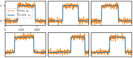
Figure 1: Examples of training pairs $(x_{i},y_{i})$ for image denoising.

2.3 Approximate Solutions

2.3.1 Gradient Descent

For simplicity we drop the dependence on $i$ for the remainder of this section.

The lower-level problem (3) can be solved with gradient descent (GD) which converges linearly for $L$-smooth and $\mu$-strongly convex problems. One can show (e.g. Chambolle2016actanumerica (3)) that GD

$$x^{k+1}=x^{k}-\tau\nabla\Phi(x^{k}),$$ (14)

with $\tau=1/L$, converges linearly to the unique solution $x^{*}$ of (3). More precisely, for all $k\in\mathbb{N}$ we have (Beck2017, 40, Theorem 10.29)

$$\|x^{k}-x^{*}\|^{2}\leq\left(1-\mu/L\right)^{k}\|x^{0}-x^{*}\|^{2}\,.$$ (15)

Moreover, if one has a good estimate of the strong convexity constant $\mu$, then it is better to choose $\tau=2/(L+\mu)$, which gives an improved linear rate (Nesterov2004, 41, Theorem 2.1.15)

$$\|x^{k}-x^{*}\|^{2}\leq(1-\mu/L)^{2k}\|x^{0}-x^{*}\|^{2}.$$ (16)

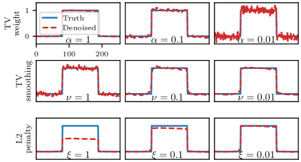
Figure 2: Examples of denoised data using model (8) obtained by running GD with a tolerance of $\|x^{k}-x^{*}\|\leq 1\mathrm{e}{-6}$. The data $(x_{i},y_{i})$ is the top-left image in Figure 1. Top: results with $\alpha=1,0.1,0.01$ (left to right) with $\nu=\xi=1\mathrm{e}{-3}$ throughout. Middle: results with $\nu=1,0.1,0.01$ (left to right) with $\alpha=1$ and $\xi=1\mathrm{e}{-3}$ throughout. Bottom: results with $\xi=1,0.1,0.01$ (left to right) with $\alpha=1$ and $\nu=1\mathrm{e}{-3}$ throughout.

2.3.2 FISTA

Similarly, we can use FISTA Beck2009 (42) to approximately solve the lower-level problem. FISTA applied to a smooth objective with convex constraints is a modification of Nesterov1983 (43) and can be formulated as the iteration

$$\begin{aligned} t_{k+1}&=\frac{1-qt_{k}^{2}+\sqrt{(1-qt_{k}^{2})^{2}+4t_{k}^{2}}}{2},\\ \beta_{k+1}&=\frac{(t_{k}-1)(1-t_{k+1}q)}{t_{k+1}(1-q)},\\ z^{k+1}&=x^{k}+\beta_{k+1}(x^{k}-x^{k-1}),\\ x^{k+1}&=z^{k+1}-\tau\nabla\Phi(z^{k+1}),\\ \end{aligned}$$ (17)

where $q:=\tau\mu$, and we choose $\tau=1/L$ and $t_{0}=0$ (Chambolle2016actanumerica, 3, Algorithm 5). We then achieve linear convergence with (Chambolle2016actanumerica, 3, Theorem 4.10)

$$\Phi(x^{k})-\Phi(x^{*})\leq\left(1-\sqrt{q}\right)^{k}\left[\frac{L}{2}(1+\sqrt{q})\|x^{0}-x^{*}\|^{2}\right],$$ (18)

and so, since $\Phi(x^{k})-\Phi(x^{*})\geq(\mu/2)\|x^{k}-x^{*}\|^{2}$ from $\mu$-strong convexity, we get

$$\|x^{k}-x^{\ast}\|^{2}\leq\left(1-\sqrt{\frac{\mu}{L}}\right)^{k}\left[\frac{L}{\mu}\left(1+\sqrt{\frac{\mu}{L}}\right)\|x^{0}-x^{*}\|^{2}\right]\,.$$ (19)

2.3.3 Ensuring accuracy requirements

We will need to be able to solve the lower-level problem to sufficient accuracy that we can guarantee $\|x^{k}-x^{*}\|^{2}\leq\epsilon$, for a suitable accuracy $\epsilon>0$. We can guarantee this accuracy by ensuring we terminate with $k$ sufficiently large, given an estimate $\|x^{0}-x^{*}\|^{2}$, using the a-priori bounds (15) or (19). A simple alternative is to use the a-posteriori bound $\|x-x^{*}\|\leq\|\nabla\Phi(x)\|/\mu$ for all $x$ (a consequence of (Beck2009, 42, Theorem 5.24(iii))), and terminate once

$$\|\nabla\Phi(x^{k})\|^{2}/\mu^{2}\leq\epsilon.$$ (20)

To compare these two options, we consider two test problems: i) a version of Nesterov’s quadratic (Nesterov2004, 41, Section 2.1.4) in $\mathbb{R}^{10}$, and ii) 1D image denoising. Nesterov’s quadratic is defined as

$$\Phi(x) :=\frac{\widetilde{\mu}(Q-1)}{8}\left(x^{T}Ax-2x_{1}\right)+\frac{\widetilde{\mu}}{2}\|x\|^{2},$$

$$\text{where}\>A:=\begin{bmatrix}2&-1&&\\ -1&2&\ddots&\\ &\ddots&\ddots&-1\\ &&-1&2\end{bmatrix},$$ (21)

for $x\in\mathbb{R}^{10}$, with $\widetilde{\mu}=1$ and $Q=100$, which is $\mu$-strongly convex and $L$-smooth for $\mu\approx 3$ and $L\approx 98$; we apply no constraints, $X=\mathbb{R}^{10}$.

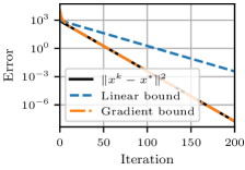
(a) GD

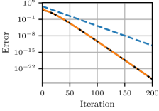
(b) FISTA

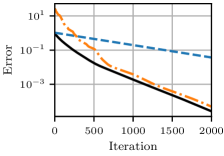
(c) GD

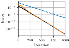
(d) FISTA

Figure 3: Comparison of a-priori linear convergence bounds (16) and (19) against the a-posteriori gradient bound (20). (a, b): 200 iterations of GD and FISTA on Nesterov’s quadratic function. (c, d): GD (2,000 iterations) and FISTA (1,000 iterations) on a 1D denoising problem.

We also consider a 1D denoising problem as in (8) with randomly-generated data $y\in\mathbb{R}^{N}$ (with $N=100$ pixels) as per Section 2.2, $\alpha=0.3$, $\nu=\xi=10^{-3}$, and $x^{*}$ estimated by running $10^{4}$ iterations of FISTA. Here, the problem is $\mu$-strongly convex and $L$-smooth with $\mu\approx 1$ and $L\approx 1,201$. We estimate the true solution $x^{*}$ by running FISTA for 10,000 iterations (which gives an upper bound estimate $\|x^{k}-x^{*}\|^{2}\leq 3\mathrm{e}{-26}$ from (20)).

In Figure 3, we compare the true error $\|x^{k}-x^{*}\|^{2}$ against the a-priori linear convergence bounds (15) or (19) with the true value of $\|x^{0}-x^{*}\|^{2}$, and the a-posteriori gradient bound (20). In both cases, the gradient-based bound (20) provides a much tighter estimate of the error, particularly for high accuracy requirements. Thus, in our numerical results, we terminate the lower-level solver as soon (20) is achieved for our desired tolerance. The gradient-based bound has the additional advantage of not requiring an a priori estimate of $\|x^{0}-x^{*}\|$. For comparison, in our results below we will also consider terminating GD/FISTA after a fixed number of iterations.

3 Dynamic Accuracy DFO Algorithm

3.1 DFO Background

Since evaluating $\hat{x}_{i}(\theta)$ in the upper-level problem (2) is only possible with some error (it is computed by running an iterative process), it is not straightforward or cheap to evaluate $\partial\hat{x}_{i}(\theta)$. Hence for solving (2) we turn to DFO techniques, and specifically consider those which exploit the nonlinear least-squares problem structure. In this section we outline a model-based DFO method for nonlinear least-squares problems Cartis2019a (24), a trust-region method based on the classical (derivative-based) Gauss–Newton method (Nocedal2006, 44, Chapter 10). However, these approaches are based on having access to exact function evaluations, and so we augment this with a standard approach for dynamic accuracy trust-region methods (Conn2000, 26, Chapter 10.6); this was previously considered for general model-based DFO methods in Conn2012 (25).

Here, we write the upper-level problem (2) in the general form

$$\min_{\theta\in\mathbb{R}^{d}}f(\theta):=\frac{1}{n}\|r(\theta)\|^{2}=\frac{1}{n}\sum_{i=1}^{n}r_{i}(\theta)^{2},$$ (22)

where $r_{i}(\theta):=\|\hat{x}_{i}(\theta)-x_{i}\|$ and $r(\theta):=[r_{1}(\theta),\ldots,r_{n}(\theta)]^{T}$. Without loss of generality, we do not include a regularization term $\mathcal{J}(\theta)$; we can incorporate this term by defining $r_{n+1}(\theta):=\sqrt{\mathcal{J}(\theta)}$ and then taking $r(\theta):=[r_{1}(\theta),\ldots,r_{n+1}(\theta)]^{T}$, for instance.

The upper-level objective (22) assumes access to exact evaluations of the lower-level objective $r_{i}(\theta)$, which is not achievable in practice. We therefore assume we only have access to inaccurate evaluations $\widetilde{x}_{i}(\theta)\approx\hat{x}_{i}(\theta)$, giving $\widetilde{r}_{i}(\theta):=\|\widetilde{x}_{i}(\theta)-x_{i}\|$, $\widetilde{r}(\theta):=[\widetilde{r}_{1}(\theta),\ldots,\widetilde{r}_{n}(\theta)]^{T}$, and $\widetilde{f}(\theta):=\frac{1}{n}\|\widetilde{r}(\theta)\|^{2}$.

Our overall algorithmic framework is based on trust-region methods, where at each iteration $k$ we construct a model $m^{k}$ for the objective which we hope is accurate in a neighborhood of our current iterate $\theta^{k}$. Simultaneously we maintain a trust-region radius $\Delta^{k}>0$, which tracks the size of the neighborhood of $\theta^{k}$ where we expect $m^{k}$ to be accurate. Our next iterate is determined by minimizing the model $m^{k}$ within a ball of size $\Delta^{k}$ around $\theta^{k}$.

Usually $m^{k}$ is taken to be a quadratic function (e.g. a second-order Taylor series for $f$ about $\theta^{k}$). However here we use the least-squares problem structure (22) and construct a linear model

$$r(\theta^{k}+s)\approx\widetilde{r}(\theta^{k}+s)\approx M^{k}(s):=\widetilde{r}(\theta^{k})+J^{k}s,$$ (23)

where $\widetilde{r}(\theta^{k})$ is our approximate evaluation of $r(\theta^{k})$ and $J^{k}\in\mathbb{R}^{n\times d}$ is a matrix approximating $\partial r(\theta^{k})^{T}$. We construct $J^{k}$ by interpolation: we maintain an interpolation set $z^{0},\ldots,z^{d}\in\mathbb{R}^{d}$ (where $z^{0}:=\theta^{k}$ at each iteration $k$) and choose $J^{k}$ so that

$$M^{k}(z^{t}-\theta^{k})=\widetilde{r}(z^{t}),\qquad\forall t=1,\ldots,d.$$ (24)

This condition ensures that our linear model $M^{k}$ exactly interpolates $\widetilde{r}$ at our interpolation points $z^{t}$ (i.e. the second approximation in (23) is exact for each $s=z^{t}-\theta^{k}$). We can therefore find $J^{k}$ by solving the $d\times d$ linear system (with $n$ right-hand sides):

$$\begin{bmatrix}(z^{1}-\theta^{k})&\cdots&(z^{d}-\theta^{k})\end{bmatrix}^{T}g^{k}_{i}=\begin{bmatrix}\widetilde{r}_{i}(z^{1})-\widetilde{r}_{i}(\theta^{k})\\ \vdots\\ \widetilde{r}_{i}(z^{d})-\widetilde{r}_{i}(\theta^{k})\end{bmatrix},$$ (25)

for all $i=1,\ldots,n$, where $g^{k}_{i}\in\mathbb{R}^{d}$ is the $i$-th row of $J^{k}$. The model $M^{k}$ gives a natural quadratic model for the full objective $f$:

$$f(\theta^{k}+s)\approx m^{k}(s):=\frac{1}{n}\|M^{k}(s)\|^{2} =\widetilde{f}(\theta^{k})+(g^{k})^{T}s$$

$$\quad+\frac{1}{2}s^{T}H^{k}s,$$ (26)

where $g^{k}:=\frac{2}{n}(J^{k})^{T}\widetilde{r}(\theta^{k})$ and $H^{k}:=\frac{2}{n}(J^{k})^{T}J^{k}$. We compute a tentative step $s^{k}$ as a(n approximate) minimizer of the trust-region subproblem

$$\min_{s\in\mathbb{R}^{d}}m^{k}(s),\qquad\text{subject to}\qquad\|s\|\leq\Delta^{k}.$$ (27)

There are a variety of efficient algorithms for computing $s^{k}$ (Conn2000, 26, Chapter 7). Finally, we evaluate $\widetilde{f}(\theta^{k}+s^{k})$ and decide whether to accept or reject the step (i.e. set $\theta^{k+1}=\theta^{k}+s^{k}$ or $\theta^{k+1}=\theta^{k}$) depending on the ratio

$$\rho^{k}=\frac{\text{actual reduction}}{\text{predicted reduction}}:=\frac{f(\theta^{k})-f(\theta^{k}+s^{k})}{m^{k}(0)-m^{k}(s^{k})}.$$ (28)

Although we would like to accept/reject using $\rho^{k}$, in reality we only observe the approximation

$$\widetilde{\rho}^{k}:=\frac{\widetilde{f}(\theta^{k})-\widetilde{f}(\theta^{k}+s^{k})}{m^{k}(0)-m^{k}(s^{k})},$$ (29)

and so we use this instead.

This gives us the key components of a standard trust-region algorithm. We have two extra considerations in our context: the accuracy of our derivative-free model (26) and the lack of exact evaluations of the objective.

Firstly, we require a procedure to verify if our model (26) is sufficiently accurate inside the trust-region, and if not, modify the model to ensure its accuracy. We discuss this in Section 3.2. The notion of ‘sufficiently accurate’ we use here is that $m^{k}$ is as good an approximation to $f$ as a first-order Taylor series (up to constant factors), which we call ‘fully linear’.

Definition 3 (Fully linear model)

The model $m^{k}$ (26) is a fully linear model for $f(\theta)$ in $B(\theta^{k},\Delta^{k})$ if there exist constants $\kappa_{\rm ef},\kappa_{\rm eg}>0$ (independent of $\theta^{k}$ and $\Delta^{k}$) such that

$$|f(\theta^{k}+s)-m^{k}(s)| \leq\kappa_{\rm ef}(\Delta^{k})^{2},$$ (30)

$$\|\nabla f(\theta^{k}+s)-\nabla m^{k}(s)\| \leq\kappa_{\rm eg}\Delta^{k},$$ (31)

for all $\|s\|\leq\Delta^{k}$.

Secondly, we handle the inaccuracy in objective evaluations by ensuring $\widetilde{f}(\theta^{k})$ and $\widetilde{f}(\theta^{k}+s^{k})$ are evaluated to a sufficiently high accuracy when we compute $\widetilde{\rho}^{k}$ (29). Specifically, suppose we know that $|\widetilde{f}(\theta^{k})-f(\theta^{k})|\leq\delta^{k}$ and $|\widetilde{f}(\theta^{k}+s^{k})-f(\theta^{k}+s^{k})|\leq\delta^{k}_{+}$ for some accuracies $\delta^{k}$ and $\delta^{k}_{+}$. Throughout, we use $\delta^{k}$ and $\delta^{k}_{+}$ to refer to the accuracies with which $\widetilde{f}(\theta^{k})$ and $\widetilde{f}(\theta^{k}+s^{k})$ have been evaluated, in the sense above. Before we compute $\widetilde{\rho}^{k}$, we first ensure that

$$\max(\delta^{k},\delta^{k}_{+})\leq\eta_{1}^{\prime}\left[m^{k}(0)-m^{k}(s^{k})\right],$$ (32)

where $\eta_{1}^{\prime}>0$ is an algorithm parameter. We achieve this by running the lower-level solver for a sufficiently large number of iterations.

The full upper-level algorithm is given in Algorithm 1; it is similar to the approach in Conn2012 (25), the DFO method (Conn2009, 18, Algorithm 10.1)—adapted for the least-squares problem structure—and the (derivative-based) dynamic accuracy trust-region method (Conn2000, 26, Algorithm 10.6.1).

1:Inputs: Starting point $\theta^{0}\in\mathbb{R}^{n}$, initial trust region radius $0<\Delta^{0}\leq\Delta_{\max}$.

2:Parameters: strictly positive values $\Delta_{\max},\gamma_{\rm dec},\gamma_{\rm inc},\eta_{1},\eta_{2},\eta_{1}^{\prime},\epsilon$ satisfying $\gamma_{\rm dec}<1<\gamma_{\rm inc}$, $\eta_{1}\leq\eta_{2}<1$, and $\eta_{1}^{\prime}<\min(\eta_{1},1-\eta_{2})/2$.

3:Select an arbitrary interpolation set and construct $m^{0}$ (26).

4:for $k=0,1,2,\ldots$ do

5:    repeat

6:         Evaluate $\widetilde{f}(\theta^{k})$ to sufficient accuracy that (32) holds with $\eta_{1}^{\prime}$ (using $s^{k}$ from the previous iteration of this inner repeat/until loop). Do nothing in the first iteration of this repeat/until loop.

7:         if $\|g^{k}\|\leq\epsilon$ then

8:             By replacing $\Delta^{k}$ with $\gamma_{\rm dec}^{i}\Delta^{k}$ for $i=0,1,2,\ldots$, find $m^{k}$ and $\Delta^{k}$ such that $m^{k}$ is fully linear in $B(\theta^{k},\Delta^{k})$ and $\Delta^{k}\leq\|g^{k}\|$. [criticality phase]

9:         end if

10:         Calculate $s^{k}$ by (approximately) solving (27).

11:    until the accuracy in the evaluation of $\widetilde{f}(\theta^{k})$ satisfies (32) with $\eta_{1}^{\prime}$ [accuracy phase]

12:    Evaluate $\widetilde{r}(\theta^{k}+s^{k})$ so that (32) is satisfied with $\eta_{1}^{\prime}$ for $\widetilde{f}(\theta^{k}+s^{k})$, and calculate $\widetilde{\rho}^{k}$ (29).

13:    Set $\theta^{k+1}$ and $\Delta^{k+1}$ as:

$$\theta^{k+1}=\begin{cases}\theta^{k}+s^{k},&\text{$\widetilde{\rho}^{k}\geq\eta_{2}$, or $\widetilde{\rho}^{k}\geq\eta_{1}$ and $m^{k}$}\\ &\text{fully linear in $B(\theta^{k},\Delta^{k})$,}\\ \theta^{k},&\text{otherwise},\end{cases}$$ (33)

and

$$\Delta^{k+1}=\begin{cases}\min(\gamma_{\rm inc}\Delta^{k},\Delta_{\max}),&\text{$\widetilde{\rho}^{k}\geq\eta_{2}$, }\\ \Delta^{k},&\text{$\widetilde{\rho}^{k}<\eta_{2}$ and $m^{k}$ not }\\ &\text{fully linear in $B(\theta^{k},\Delta^{k})$,}\\ \gamma_{\rm dec}\Delta^{k},&\text{otherwise}.\end{cases}$$ (34)

14:    If $\theta^{k+1}=\theta^{k}+s^{k}$, then build $m^{k+1}$ by adding $\theta^{k+1}$ to the interpolation set (removing an existing point). Otherwise, set $m^{k+1}=m^{k}$ if $m^{k}$ is fully linear in $B(\theta^{k},\Delta^{k})$, or form $m^{k+1}$ by making $m^{k}$ fully linear in $B(\theta^{k+1},\Delta^{k+1})$.

15:end for

Algorithm 1 Dynamic accuracy DFO algorithm for (22).

Our main convergence result is the below.

Theorem 3.1

Suppose Assumptions 2 and 3 hold. Then if

$$K >\left\lfloor\left(2+2\frac{\log\gamma_{\rm inc}}{|\log\gamma_{\rm dec}|}\right)\frac{2(\kappa_{\rm eg}+1)f(\theta^{0})}{(\eta_{1}-2\eta_{1}^{\prime})\epsilon\Delta_{\min}}\right.$$

$$\qquad\qquad\qquad\qquad\qquad\left.+2\frac{\log(\Delta^{0}/\Delta_{\min})}{|\log\gamma_{\rm dec}|}\right\rfloor,$$ (35)

with $\kappa_{\rm eg}$ and $\Delta_{\min}$ given by Lemmas 1 and 8 respectively, then $\min_{k=0,\ldots,K}\|\nabla f(\theta^{k})\|<\epsilon$.

We summarize Theorem 3.1 as follows, noting that the iteration and evaluation counts match the standard results for model-based DFO (e.g. Cartis2019a (24, 45)).

Corollary 1

Suppose the assumptions of Theorem 3.1 hold. Then Algorithm 1 is globally convergent; i.e.

$$\lim_{k\to\infty}\|\nabla f(\theta^{k})\|=0.$$ (36)

Also, if $\epsilon\in(0,1]$, then the number of iterations before $\|\nabla f(\theta^{k})\|<\epsilon$ for the first time is at most $\mathcal{O}(\kappa^{3}\epsilon^{-2})$ and the number of evaluations of $\widetilde{r}(\theta)$ is at most $\mathcal{O}(d\kappa^{3}\epsilon^{-2})$, where $\kappa:=\max(\kappa_{\rm ef},\kappa_{\rm eg},\kappa_{H})$.

We note that since $\theta^{k}\in\mathcal{B}$ and $\mathcal{B}$ is bounded from Assumption 2 (and closed by continuity of $f$), then by Corollary 1 and compactness there exists a subsequence of iterates $\{\theta_{k_{i}}\}_{i\in\mathbb{N}}$ which converges to a stationary point of $f$. However, there are relatively few results which prove convergence of the full sequence of iterates for nonconvex trust-region methods (see (Conn2000, 26, Theorem 10.13) for a restricted result in the derivative-based context).

3.2 Guaranteeing Model Accuracy

As described above, we need a process to ensure that $m^{k}$ (26) is a fully linear model for $f$ inside the trust region $B(\theta^{k},\Delta^{k})$. For this, we need to consider the geometry of the interpolation set.

Definition 4

The Lagrange polynomials of the interpolation set $\{z^{0},z^{1},\ldots,z^{d}\}$ are the linear polynomials $\ell_{t}$, $t=0,\ldots,d$ such that $\ell_{t}(z^{s})=\delta_{s,t}$ for all $s,t=0,\ldots,d$.

The Lagrange polynomials of $\{z^{0},\ldots,z^{d}\}$ exist and are unique whenever the matrix in (25) is invertible. The required notion of ‘good geometry’ is given by the below definition (where small $\Lambda$ indicates better geometry).

Definition 5 ($\Lambda$-poisedness)

For $\Lambda>0$, the interpolation set $\{z^{0},\ldots,z^{d}\}$ is $\Lambda$-poised in $B(\theta^{k},\Delta^{k})$ if $|\ell_{t}(\theta^{k}+s)|\leq\Lambda$ for all $t=0,\ldots,d$ and all $\|s\|\leq\Delta^{k}$.

The below result confirms that, provided our interpolation set has sufficiently good geometry, and our evaluations $\widetilde{r}(\theta^{k})$ and $\widetilde{r}(y^{t})$ are sufficiently accurate, our interpolation models are fully linear.

Assumption 2

The extended level set

$$\mathcal{B}:=\{z:\text{$z\in B(\theta,\Delta_{\max})$ for some $\theta$ with $f(\theta)\leq f(\theta^{0})$}\},$$ (37)

is bounded, and $r(\theta)$ is continuously differentiable and $\partial r(\theta)$ is Lipschitz continuous with constant $L_{J}$ in $\mathcal{B}$.

In particular, Assumption 2 implies that $r(\theta)$ and $\partial r(\theta)$ are uniformly bounded in the same region—that is, $\|r(\theta)\|\leq r_{\max}$ and $\|\partial r(\theta)\|\leq J_{\max}$ for all $\theta\in\mathcal{B}$—and $f$ (22) is $L$-smooth in $\mathcal{B}$ (Cartis2019a, 24, Lemma 3.2).

We note that $\mathcal{B}$ in Assumption 2 is bounded whenever the regularizer $\mathcal{J}$ is coercive, such as in Section 4.4. This may also be replaced by the weaker assumption that $r$ and $\partial r$ are uniformly bounded on $\mathcal{B}$ (and $\mathcal{B}$ need not be bounded) (Cartis2019a, 24, Assumption 3.1), and there are theoretical results which give this for some inverse problems in image restoration DeLosReyes2016 (46). In our numerical experiments, we enforce upper and lower bounds on $\theta$, which also yields the uniform boundedness of $r$ and $\partial r$. Also, we note that if $r_{i}(\theta)=\|\hat{x}_{i}(\theta)-x_{i}\|$ is not itself $L$-smooth, we can instead treat each entry of $\hat{x}_{i}(\theta)-x_{i}$ as a separate term in (22).

Lemma 1

Suppose Assumption 2 holds and $\Delta^{k}\leq\Delta_{\max}$. If the interpolation set $\{z^{0}:=\theta^{k},z^{1},\ldots,z^{d}\}$ is $\Lambda$-poised in $B(\theta^{k},\Delta^{k})$ and for each evaluation $t=0,\ldots,d$ and each $i=1,\ldots,n$ we have

$$\|\widetilde{x}_{i}(z^{t})-\hat{x}_{i}(z^{t})\|\leq c(\Delta^{k})^{2},$$ (38)

for some $c>0$, then the corresponding models $M^{k}$ (23) and $m^{k}$ (26) are fully linear models for $r(\theta)$ and $f(\theta)$ respectively.

Proof

This is a straightforward extension of (Cartis2019a, 24, Lemma 3.3), noting that

$$|\widetilde{r}_{i}(z^{t})-r_{i}(z^{t})|\leq\|\widetilde{x}_{i}(z^{t})-\hat{x}_{i}(z^{t})\|,\qquad\forall i=1,\ldots,n,$$ (39)

and so (38) gives $\|\widetilde{r}(z^{t})-r(z^{t})\|\leq c\sqrt{n}(\Delta^{k})^{2}$ for all $t=0,\ldots,d$.

We conclude by noting that for any $\Lambda>1$ there are algorithms available to determine if a set is $\Lambda$-poised, and if it is not, change some interpolation points to make it so; details may be found in (Conn2009, 18, Chapter 6), for instance.

3.3 Lower-Level Objective Evaluations

We now consider the accuracy requirements that Algorithm 1 imposes on our lower-level objective evaluations. In particular, we require the ability to satisfy (32), which imposes requirements on the error in the calculated $\widetilde{f}$, rather than the lower-level evaluations $\widetilde{r}$. The connection between errors in $\widetilde{r}$ and $\widetilde{f}$ is given by the below result.

Lemma 2

Suppose we compute $\widetilde{x}_{i}(\theta)$ satisfying $\|\widetilde{x}_{i}(\theta)-\hat{x}_{i}(\theta)\|\leq\delta_{x}$ for all $i=1,\ldots,n$. Then we have

$$|\widetilde{f}(\theta)-f(\theta)| \leq 2\sqrt{\widetilde{f}(\theta)}\>\delta_{x}+\delta_{x}^{2}$$

$$\text{and}\quad|\widetilde{f}(\theta)-f(\theta)|\leq 2\sqrt{f(\theta)}\>\delta_{x}+\delta_{x}^{2}.$$ (40)

Moreover, if $\|\widetilde{x}_{i}(\theta)-\hat{x}_{i}(\theta)\|\leq\sqrt{\widetilde{f}(\theta)+\delta_{f}}-\sqrt{\widetilde{f}(\theta)}$ for $i=1,\ldots,n$, then $|\widetilde{f}(\theta)-f(\theta)|\leq\delta_{f}$.

Proof

Letting $\epsilon(\theta):=\widetilde{r}(\theta)-r(\theta)$, we have

$$f(\theta) =\frac{1}{n}\|\widetilde{r}(\theta)-\epsilon(\theta)\|^{2},$$ (41)

$$=\widetilde{f}(\theta)-\frac{2}{n}\epsilon(\theta)^{T}\widetilde{r}(\theta)+\frac{1}{n}\|\epsilon(\theta)\|^{2},$$ (42)

and hence

$$|f(\theta)-\widetilde{f}(\theta)| \leq\frac{2}{n}\|\epsilon(\theta)\|\|\widetilde{r}(\theta)\|+\frac{1}{n}\|\epsilon(\theta)\|^{2},$$ (43)

$$\leq\frac{2}{n}\sqrt{n}\|\epsilon(\theta)\|_{\infty}\sqrt{n\widetilde{f}(\theta)}+\|\epsilon(\theta)\|_{\infty}^{2},$$ (44)

and the first part of (40) follows since $\|\epsilon(\theta)\|_{\infty}\leq\delta_{x}$ from (39). The second part of (40) follows from an identical argument but writing $\widetilde{f}(\theta)=\frac{1}{n}\|r(\theta)+\epsilon(\theta)\|^{2}$, and the final conclusion follows immediately from the first part of (40).

We construct these bounds to rely mostly on $\widetilde{f}(\theta)$, since this is the value which is observed by the algorithm (rather than the true value $f(\theta)$). From the concavity of $\sqrt{\cdot}$, if $\widetilde{f}(\theta)$ is larger then $\|\widetilde{x}_{i}(\theta)-\hat{x}_{i}(\theta)\|$ must be smaller to achieve the same $\delta_{f}$.

Lastly, we note the key reason why we require (32): it guarantees that our estimate $\widetilde{\rho}^{k}$ of $\rho^{k}$ is not too inaccurate.

Lemma 3

Suppose $|\widetilde{f}(\theta^{k})-f(\theta^{k})|\leq\delta^{k}$ and $|\widetilde{f}(\theta^{k}+s^{k})-f(\theta^{k}+s^{k})|\leq\delta^{k}_{+}$. If (32) holds, then $|\widetilde{\rho}^{k}-\rho^{k}|\leq 2\eta_{1}^{\prime}$.

Proof

Follows immediately from (29) and (28); see (Conn2000, 26, Section 10.6.1).

3.4 Convergence and Worst-Case Complexity

We now prove the global convergence of Algorithm 1 and analyse its worst-case complexity (i.e. the number of iterations required to achieve $\|\nabla f(\theta^{k})\|\leq\epsilon$ for the first time).

Assumption 3

The computed trust-region step $s^{k}$ satisfies

$$m^{k}(0)-m^{k}(s^{k})\geq\frac{1}{2}\|g^{k}\|\min\left(\Delta^{k},\frac{\|g^{k}\|}{\|H^{k}\|+1}\right),$$ (45)

and there exists $\kappa_{H}\geq 1$ such that $\|H^{k}\|+1\leq\kappa_{H}$ for all $k$.

Assumption 3 is standard and the condition (45) easy to achieve in practice (Conn2000, 26, Chapter 6.3).

Firstly, we must show that the inner loops for the criticality and accuracy phases terminate. We begin with the criticality phase, and then consider the accuracy phase.

Lemma 4 ((Cartis2019a, 24, Lemma B.1))

Suppose Assumption 2 holds and $\|\nabla f(\theta^{k})\|\geq\epsilon>0$. Then the criticality phase terminates in finite time with

$$\min\left(\Delta^{k}_{\rm init},\frac{\gamma_{\rm dec}\epsilon}{\kappa_{\rm eg}+1}\right)\leq\Delta^{k}\leq\Delta^{k}_{\rm init},$$ (46)

where $\Delta^{k}_{\rm init}$ is the value of $\Delta^{k}$ before the criticality phase begins.

Lemma 5 ((Cartis2019a, 24, Lemma 3.7))

Suppose Assumption 2 holds. Then in all iterations we have $\|g^{k}\|\geq\min(\epsilon,\Delta^{k})$. Also, if $\|\nabla f(\theta^{k})\|\geq\epsilon>0$, then $\|g^{k}\|\geq\epsilon/(\kappa_{\rm eg}+1)>0$.

We note that our presentation of the criticality phase here can be made more general by allowing $\|g^{k}\|\geq\epsilon_{C}\neq\epsilon$ as the entry test, setting $\Delta^{k}$ to $\omega^{i}\Delta^{k}$ for some $\omega\in(0,1)$ possibly different to $\gamma_{\rm dec}$, and having an exit test $\Delta^{k}\leq\mu\|g^{k}\|$ for some $\mu>0$. All the below results hold under these assumptions, with modifications as per Cartis2019a (24).

Lemma 6

If Assumptions 2 and 3 hold and $\|\nabla f(\theta^{k})\|\geq\epsilon>0$, then the accuracy phase terminates in finite time (i.e. line 12 of Algorithm 1 is eventually called)

Proof

From Lemma 5 we have $\|g^{k}\|\geq\epsilon/(\kappa_{\rm eg}+1)$, and the result then follows from (Conn2000, 26, Lemma 10.6.1).

We now collect some key preliminary results required to establish complexity bounds.

Lemma 7

Suppose Assumptions 2 and 3 hold, $m^{k}$ is fully linear in $B(\theta^{k},\Delta^{k})$ and

$$\Delta^{k} \leq c_{0}\|g^{k}\|,$$

$$\text{where}\quad c_{0}:=\min\left(\frac{1-\eta_{2}-2\eta_{1}^{\prime}}{4\kappa_{\rm ef}},\frac{1}{\kappa_{H}}\right)>0,$$ (47)

then $\widetilde{\rho}^{k}\geq\eta_{2}$.

Proof

We compute

$$|\rho^{k}-1| =\left|\frac{(f(\theta^{k})-f(\theta^{k}+s^{k}))-(m^{k}(0)-m^{k}(s^{k}))}{m^{k}(0)-m^{k}(s^{k})}\right|,$$ (48)

$$\leq\frac{|f(\theta^{k}+s^{k})-m^{k}(s^{k})|}{|m^{k}(0)-m^{k}(s^{k})|}+\frac{|f(\theta^{k})-m^{k}(0)|}{|m^{k}(0)-m^{k}(s^{k})|}.$$ (49)

Since $\Delta^{k}\leq\|g^{k}\|/\kappa_{H}$, from Assumption 3 we have

$$m^{k}(0)-m^{k}(s^{k})\geq\frac{1}{2}\|g^{k}\|\Delta^{k}.$$ (50)

From this and full linearity, we get

$$|\rho^{k}-1|\leq 2\left(\frac{2\kappa_{\rm ef}(\Delta^{k})^{2}}{\|g^{k}\|\Delta^{k}}\right)\leq 1-\eta_{2}-2\eta_{1}^{\prime},$$ (51)

and so $\rho^{k}\geq\eta_{2}+2\eta_{1}^{\prime}$, hence $\widetilde{\rho}^{k}\geq\eta_{2}$ from Lemma 3.

Lemma 8

Suppose Assumptions 2 and 3 hold. Suppose $\|\nabla f(\theta^{k})\|\geq\epsilon$ for all $k=0,\ldots,k_{\epsilon}$ and some $\epsilon\in(0,1)$. Then, for all $k\leq k_{\epsilon}$,

$$\Delta^{k}\geq\Delta_{\min}:=\gamma_{\rm dec}\min\left(\Delta^{0},\frac{c_{0}\epsilon}{\kappa_{\rm eg}+1},\frac{\gamma_{\rm dec}\epsilon}{\kappa_{\rm eg}+1}\right)>0.$$ (52)

Proof

As above, we let $\Delta^{k}_{\rm init}$ and $m^{k}_{\rm init}$ denote the values of $\Delta^{k}$ and $m^{k}$ before the criticality phase (i.e. $\Delta^{k}_{\rm init}=\Delta^{k}$ and $m^{k}_{\rm init}=m^{k}$ if the criticality phase is not called). From Lemma 5, we know $\|g^{k}\|\geq\epsilon/(\kappa_{\rm eg}+1)$ for all $k\leq k_{\epsilon}$. Suppose by contradiction $k\leq k_{\epsilon}$ is the first iteration such that $\Delta^{k}<\Delta_{\min}$. Then from Lemma 4,

$$\frac{\gamma_{\rm dec}\epsilon}{\kappa_{\rm eg}+1}\geq\Delta_{\min}>\Delta^{k}\geq\min\left(\Delta^{k}_{\rm init},\frac{\gamma_{\rm dec}\epsilon}{\kappa_{\rm eg}+1}\right),$$ (53)

and so $\Delta^{k}\geq\Delta^{k}_{\rm init}$; hence $\Delta^{k}=\Delta^{k}_{\rm init}$. That is, either the criticality phase is not called, or terminates with $i=0$ (in this case, the model $m^{k}$ is formed simply by making $m^{k}_{\rm init}$ fully linear in $B(\theta^{k},\Delta^{k})=B(\theta^{k},\Delta^{k}_{\rm init})$).

If the accuracy phase loop occurs, we go back to the criticality phase, which can potentially happen multiple times. However, since the only change is that $\widetilde{r}(\theta^{k})$ is evaluated to higher accuracy, incorporating this information into the model $m^{k}$ can never destroy full linearity. Hence, after the accuracy phase, by the same reasoning as above, either one iteration of the criticality phase occurs (i.e. $m^{k}$ is made fully linear) or it is not called. If the accuracy phase is called multiple times and the criticality phase occurs multiple times, all times except the first have no effect (since the accuracy phase can never destroy full linearity). Thus $\Delta^{k}$ is unchanged by the accuracy phase.

Since $\Delta_{\min}<\Delta^{0}_{\rm init}$, we have $k\geq 1$. As $k$ is the first iteration such that $\Delta^{k}<\Delta_{\min}$ and $\Delta^{k}=\Delta^{k}_{\rm init}$, we must have $\Delta^{k}_{\rm init}=\gamma_{\rm dec}\Delta^{k-1}$ (as this is the only other way $\Delta^{k}$ can be reduced). Therefore $\Delta^{k-1}=\Delta^{k}/\gamma_{\rm dec}<\Delta_{\min}/\gamma_{\rm dec}$, and so

$$\Delta^{k-1}\leq\min\left(\frac{c_{0}\epsilon}{\kappa_{\rm eg}+1},\frac{\gamma_{\rm dec}\epsilon}{\kappa_{\rm eg}+1}\right).$$ (54)

We then have $\Delta^{k-1}\leq c_{0}\epsilon/(\kappa_{\rm eg}+1)\leq c_{0}\|g^{k-1}\|$, and so by (7) either $\widetilde{\rho}^{k}\geq\eta_{2}$ or $m^{k-1}$ is not fully linear. Either way, we set $\Delta^{k}_{\rm init}\geq\Delta^{k-1}$ in (34). This contradicts $\Delta^{k}_{\rm init}=\gamma_{\rm dec}\Delta^{k-1}$ above, and we are done.

We now bound the number of iterations of each type. Specifically, we suppose that $k_{\epsilon}+1$ is the first $k$ such that $\|\nabla f(\theta^{k})\|\geq\epsilon$. Then, we define the sets of iterations:

• $\mathcal{S}_{\epsilon}$ is the set of iterations $k\in\{0,\ldots,k_{\epsilon}\}$ which are ‘successful’; i.e. $\widetilde{\rho}^{k}\geq\eta_{2}$, or $\widetilde{\rho}^{k}\geq\eta_{1}$ and $m^{k}$ is fully linear in $B(\theta^{k},\Delta^{k})$.

• $\mathcal{M}_{\epsilon}$ is the set of iterations $k\in\{0,\ldots,k_{\epsilon}\}$ which are ‘model-improving’; i.e. $\widetilde{\rho}^{k}<\eta_{2}$ and $m^{k}$ is not fully linear in $B(\theta^{k},\Delta^{k})$.

• $\mathcal{U}_{\epsilon}$ is the set of iterations $k\in\{0,\ldots,k_{\epsilon}\}$ which are ‘unsuccessful’; i.e. $\widetilde{\rho}^{k}<\eta_{1}$ and $m^{k}$ is fully linear in $B(\theta^{k},\Delta^{k})$.

These three sets form a partition of $\{0,\ldots,k_{\epsilon}\}$.

Proposition 1

Suppose Assumptions 2 and 3 hold. Then

$$|\mathcal{S}_{\epsilon}|\leq\frac{2(\kappa_{\rm eg}+1)f(\theta^{0})}{(\eta_{1}-2\eta_{1}^{\prime})\epsilon\Delta_{\min}}.$$ (55)

Proof

By definition of $k_{\epsilon}$, $\|\nabla f(\theta^{k})\|\geq\epsilon$ for all $k\leq k_{\epsilon}$ and so Lemma 5 and Lemma 8 give $\|g^{k}\|\geq\epsilon/(\kappa_{\rm eg}+1)$ and $\Delta^{k}\geq\Delta_{\min}$ for all $k\leq k_{\epsilon}$ respectively. For any $k\leq k_{\epsilon}$ we have

$$f(\theta^{k}) -f(\theta^{k+1})$$

$$=\rho^{k}[m^{k}(0)-m^{k}(s^{k})],$$ (56)

$$\geq\frac{1}{2}\rho^{k}\|g^{k}\|\min\left(\Delta^{k},\frac{\|g^{k}\|}{\|H^{k}\|+1}\right),$$ (57)

$$\geq\frac{1}{2}\rho^{k}\frac{\epsilon}{\kappa_{\rm eg}+1}\min\left(\Delta_{\min},\frac{\epsilon}{\kappa_{H}(\kappa_{\rm eg}+1)}\right),$$ (58)

by definition of $\rho^{k}$ and Assumption 3. If $k\in\mathcal{S}_{\epsilon}$, we know $\widetilde{\rho_{k}}\geq\eta_{1}$, which implies $\rho^{k}\geq\eta_{1}-2\eta_{1}^{\prime}>0$ from Lemma 3. Therefore

$$f(\theta^{k}) -f(\theta^{k+1})$$

$$\geq\frac{1}{2}(\eta_{1}-2\eta_{1}^{\prime})\frac{\epsilon}{\kappa_{\rm eg}+1}\min\left(\Delta_{\min},\frac{\epsilon}{\kappa_{H}(\kappa_{\rm eg}+1)}\right),$$ (59)

$$=\frac{1}{2}(\eta_{1}-2\eta_{1}^{\prime})\frac{\epsilon}{\kappa_{\rm eg}+1}\Delta_{\min},$$ (60)

for all $k\in\mathcal{S}_{\epsilon}$, where the last line follows since $\Delta_{\min}<c_{0}\epsilon/(\kappa_{\rm eg}+1)\leq\epsilon/[\kappa_{H}(\kappa_{\rm eg}+1)]$ by definition of $\Delta_{\min}$ (52) and $c_{0}$ (47).

The iterate $\theta^{k}$ is only changed on successful iterations (i.e. $\theta^{k+1}=\theta^{k}$ for all $k\notin\mathcal{S}_{\epsilon}$). Thus, as $f(\theta)\geq 0$ from the least-squares structure (22), we get

$$f(\theta^{0}) \geq f(\theta^{0})-f(\theta^{k_{\epsilon}+1}),$$ (61)

$$=\sum_{k\in\mathcal{S}_{\epsilon}}f(\theta^{k})-f(\theta^{k+1}),$$ (62)

$$\geq|\mathcal{S}_{\epsilon}|\left[\frac{1}{2}(\eta_{1}-2\eta_{1}^{\prime})\frac{\epsilon}{\kappa_{\rm eg}+1}\Delta_{\min}\right],$$ (63)

and the result follows.

We are now in a position to prove our main results.

Proof (Proof of Theorem 3.1)

To derive a contradiction, suppose that $\|\nabla f(\theta^{k})\|\geq\epsilon$ for all $k\in\{0,\ldots,K\}$, and so $\|g^{k}\|\geq\epsilon/(\kappa_{\rm eg}+1)$ and $\Delta^{k}\geq\Delta_{\min}$ by Lemma 5 and Lemma 8 respectively. Since $K\leq k_{\epsilon}$ by definition of $k_{\epsilon}$, we will try to construct an upper bound on $k_{\epsilon}$. We already have an upper bound on $|\mathcal{S}_{\epsilon}|$ from Proposition 1.

If $k\in\mathcal{S}_{\epsilon}$, we set $\Delta^{k+1}\leq\gamma_{\rm inc}\Delta^{k}$. Similarly, if $k\in\mathcal{U}_{\epsilon}$ we set $\Delta^{k+1}=\gamma_{\rm dec}\Delta^{k}$. Thus

$$\Delta_{\min}\leq\Delta^{k_{\epsilon}}\leq\Delta^{0}\gamma_{\rm inc}^{|\mathcal{S}_{\epsilon}|}\gamma_{\rm dec}^{|\mathcal{U}_{\epsilon}|}.$$ (64)

That is, $\Delta_{\min}/\Delta^{0}\leq\gamma_{\rm inc}^{|\mathcal{S}_{\epsilon}|}\gamma_{\rm dec}^{|\mathcal{U}_{\epsilon}|}$, and so

$$|\mathcal{U}_{\epsilon}| \leq\frac{\log\gamma_{\rm inc}}{|\log\gamma_{\rm dec}|}|\mathcal{S}_{\epsilon}|+\frac{\log(\Delta^{0}/\Delta_{\min})}{|\log\gamma_{\rm dec}|},$$ (65)

noting we have changed $\Delta_{\min}/\Delta^{0}<1$ to $\Delta^{0}/\Delta_{\min}>1$ and used $\log\gamma_{\rm dec}<0$, so all terms in (65) are positive. Now, the next iteration after a model-improving iteration cannot be model-improving (as the resulting model is fully linear), giving

$$|\mathcal{M}_{\epsilon}| \leq|\mathcal{S}_{\epsilon}|+|\mathcal{U}_{\epsilon}|.$$ (66)

If we combine (65) and (66) with $k_{\epsilon}\leq|\mathcal{S}_{\epsilon}|+|\mathcal{M}_{\epsilon}|+|\mathcal{U}_{\epsilon}|$, we get

$$k_{\epsilon} \leq 2(|\mathcal{S}_{\epsilon}|+|\mathcal{U}_{\epsilon}|),$$ (67)

$$\leq\left(2+2\frac{\log\gamma_{\rm inc}}{|\log\gamma_{\rm dec}|}\right)|\mathcal{S}_{\epsilon}|+2\frac{\log(\Delta^{0}/\Delta_{\min})}{|\log\gamma_{\rm dec}|},$$ (68)

which, given the bound on $|\mathcal{S}_{\epsilon}|$ (55) means $K\leq k_{\epsilon}$ is bounded above by the right-hand side of (35), a contradiction.

Proof (Proof of Corollary 1)

The iteration bound follows directly from Theorem 3.1, noting that $\Delta_{\min}=\mathcal{O}(\kappa^{-2}\epsilon)$. This also implies that $\liminf_{k\to\infty}\|\nabla f(\theta^{k})\|=0$ and so (36) holds from the same argument as in (Conn2009, 18, Theorem 10.13) without modification.

For the evaluation bound, we also need to count the number of inner iterations of the criticality phase. Suppose $\|\nabla f(\theta^{k})\|<\epsilon$ for $k=0,\ldots,k_{\epsilon}$. Similar to the above, we define: (a) $\mathcal{C}^{M}_{\epsilon}$ to be the number of criticality phase iterations corresponding to the first iteration of $i=0$ where $m^{k}$ whas not already fully linear, in iterations $0,\ldots,k_{\epsilon}$; and (b) $\mathcal{C}^{U}_{\epsilon}$ to be the number of criticality phase iterations corresponding to all other iterations $i>0$ (where $\Delta^{k}$ is reduced and $m^{k}$ is made fully linear) in iterations $0,\ldots,k_{\epsilon}$.

From Lemma 8 we have $\Delta^{k}\geq\Delta_{\min}$ for all $k\leq k_{\epsilon}$. We note that $\Delta^{k}$ is reduced by a factor $\gamma_{\rm dec}$ for every iteration of the criticality phase in $\mathcal{C}^{U}_{\epsilon}$. Thus by a more careful reasoning as we used to reach (65), we conclude

$$\Delta_{\min} \leq\Delta^{0}\gamma_{\rm inc}^{|\mathcal{S}_{\epsilon}|}\gamma_{\rm dec}^{|\mathcal{U}_{\epsilon}|+|\mathcal{C}^{U}_{\epsilon}|},$$ (69)

$$|\mathcal{C}^{U}_{\epsilon}| \leq\frac{\log\gamma_{\rm inc}}{|\log\gamma_{\rm dec}|}|\mathcal{S}_{\epsilon}|+\frac{\log(\Delta^{0}/\Delta_{\min})}{|\log\gamma_{\rm dec}|}-|\mathcal{U}_{\epsilon}|.$$ (70)

Also, after every iteration $k$ in which the first iteration of criticality phase makes $m^{k}$ fully linear, we have either a (very) successful or unsuccessful step, not a model-improving step. From the same reasoning as in Lemma 8, the accuracy phase can only cause at most one more step criticality phase in which $m^{k}$ is made fully linear, regardless of how many times it is called. Thus,

$$|\mathcal{C}^{M}_{\epsilon}| \leq 2\left(|\mathcal{S}_{\epsilon}|+|\mathcal{U}_{\epsilon}|\right).$$ (71)

Combining (70) and (71) with (65) and (66), we conclude that the number of times we make $m^{k}$ fully linear is

$$|\mathcal{M}_{\epsilon}| +|\mathcal{C}^{U}_{\epsilon}|+|\mathcal{C}^{M}_{\epsilon}|$$

$$\leq\left(3+3\frac{\log\gamma_{\rm inc}}{|\log\gamma_{\rm dec}|}\right)|\mathcal{S}_{\epsilon}|+3\frac{\log(\Delta^{0}/\Delta_{\min})}{|\log\gamma_{\rm dec}|},$$ (72)

$$\leq\left(3+3\frac{\log\gamma_{\rm inc}}{|\log\gamma_{\rm dec}|}\right)\frac{2(\kappa_{\rm eg}+1)f(\theta^{0})}{(\eta_{1}-2\eta_{1}^{\prime})\epsilon\Delta_{\min}}$$

$$\qquad\qquad\qquad\qquad+3\frac{\log(\Delta^{0}/\Delta_{\min})}{|\log\gamma_{\rm dec}|},$$ (73)

where the second inequality follows from Proposition 1.

If $\epsilon<1$, we conclude that the number of times we make $m^{k}$ fully linear before $\|\nabla f(\theta^{k})\|<\epsilon$ for the first time is the same as the number of iterations, $\mathcal{O}(\kappa^{3}\epsilon^{-2})$. Since each iteration requires one new objective evaluation (at $\theta^{k}+s^{k}$) and each time we make $m^{k}$ fully linear requires at most $\mathcal{O}(d)$ objective evaluations (corresponding to replacing the entire interpolation set), we get the stated evaluation complexity bound.

3.5 Estimating the Lower-Level Work

We have from Corollary 1 that we can achieve $\|\nabla f(\theta^{k})\|<\epsilon$ in $\mathcal{O}(\epsilon^{-2})$ evaluations of $\widetilde{r}(\theta)$. In this section, we use the fact that evaluations of $\widetilde{r}(\theta)$ come from finitely terminating a linearly-convergent procedure (i.e. strongly convex optimization) to estimate the total work required in the lower-level problem. This is particularly relevant in an imaging context, where the lower-level problem can be large-scale and poorly-conditioned; this can be the dominant cost of Algorithm 1.

Proposition 2

Suppose Assumptions 2 and 3 hold and $\|\nabla f(\theta^{k})\|\geq\epsilon$ for all $k=0,\ldots,k_{\epsilon}$ and some $\epsilon\in(0,1]$. Then for every objective evaluation in iterations $k\leq k_{\epsilon}$ it suffices to guarantee that $\|\widetilde{x}_{i}(\theta)-\hat{x}_{i}(\theta)\|=\mathcal{O}(\epsilon^{2})$ for all $i=1,\ldots,n$.

Proof

For all $k\leq k_{\epsilon}$ we have $\|g^{k}\|\geq\epsilon/(\kappa_{\rm eg}+1)$ and $\Delta^{k}\geq\Delta_{\min}$ by Lemma 5 and Lemma 8 respectively. There are two places where we require upper bounds on $\|\widetilde{x}_{i}(\theta)-\hat{x}_{i}(\theta)\|$ in our objective evaluations: ensuring $\widetilde{f}(\theta^{k})$ and $\widetilde{f}(\theta^{k}+s^{k})$ satisfy (32) and ensuring our model is fully linear using Lemma 1.

In the first case, we note that

$$m^{k}(0)-m^{k}(s^{k}) \geq\frac{1}{2}\frac{\epsilon}{\kappa_{\rm eg}+1}\min\left(\Delta_{\min},\frac{\epsilon}{\kappa_{H}(\kappa_{\rm eg}+1)}\right),$$ (74)

$$=\frac{1}{2}\frac{\epsilon}{\kappa_{\rm eg}+1}\Delta_{\min},$$ (75)

by Assumption 3 and using $\Delta_{\min}<c_{0}\epsilon/(\kappa_{\rm eg}+1)\leq\epsilon/[\kappa_{H}(\kappa_{\rm eg}+1)]$ by definition of $\Delta_{\min}$ (52) and $c_{0}$ (47). Therefore to ensure (32) it suffices to guarantee

$$\max \left(|\widetilde{f}(\theta^{k})-f(\theta^{k})|,|\widetilde{f}(\theta^{k}+s^{k})-f(\theta^{k}+s^{k})|\right)$$

$$\leq\delta_{f}^{\min}:=\frac{1}{2}\eta_{1}^{\prime}\frac{\epsilon}{\kappa_{\rm eg}+1}\Delta_{\min}.$$ (76)

From Lemma 2, specifically the second part of (40), this means to achieve (32) it suffices to guarantee

$$\|\widetilde{x}_{i}(\theta)-\hat{x}_{i}(\theta)\|\leq\sqrt{f(\theta)+\delta_{f}^{\min}}-\sqrt{f(\theta)},$$ (77)

for all $i=1,\ldots,n$, where $\theta\in\cup_{k\leq k_{\epsilon}}\{\theta^{k},\theta^{k}+s^{k}\}$. From Assumption 2 we have $f(\theta)\leq f_{\max}:=r_{\max}^{2}/n$, and so from the fundamental theorem of calculus we have

$$\sqrt{f(\theta)+\delta_{f}^{\min}} -\sqrt{f(\theta)}=\int_{f(\theta)}^{f(\theta)+\delta_{f}^{\min}}\frac{1}{2\sqrt{t}}dt,$$ (78)

$$\geq\frac{\delta_{f}^{\min}}{2\sqrt{f(\theta)+\delta_{f}^{\min}}}\geq\frac{\delta_{f}^{\min}}{2\sqrt{f_{\max}+\delta_{f}^{\min}}}.$$ (79)

Since $\epsilon<1$, $\delta_{f}^{\min}$ is bounded above by a constant and so $\sqrt{f_{\max}+\delta_{f}^{\min}}$ is bounded above. Thus (32) is achieved provided $\|\widetilde{x}_{i}(\theta)-\hat{x}_{i}(\theta)\|=\mathcal{O}(\delta_{f}^{\min})$ for all $i=1,\ldots,n$.

For the second case (ensuring full linearity), we need to guarantee (38) holds. This is achieved provided $\|\widetilde{x}_{i}(\theta)-\hat{x}_{i}(\theta)\|=\mathcal{O}(\Delta_{\min}^{2})$ for all $i=1,\ldots,n$. The result then follows by noting $\delta_{f}^{\min}=\mathcal{O}(\epsilon\Delta_{\min})$ and $\Delta_{\min}=\mathcal{O}(\epsilon)$.

Corollary 1 and Proposition 2 say that to ensure $\|\nabla f(\theta^{k})\|<\epsilon$ for some $k$, we have to perform $\mathcal{O}(d\kappa^{3}\epsilon^{-2})$ upper-level objective evaluations, each requiring accuracy at most $\|\widetilde{x}_{i}(\theta)-\hat{x}_{i}(\theta)\|=\mathcal{O}(\epsilon^{2})$ for all $i$. Since our lower-level evaluations correspond to using GD/FISTA to solve a strongly convex problem, the computational cost of each upper-level evaluation is $\mathcal{O}(n\log(\epsilon^{-2}))$ provided we have reasonable initial iterates. From this, we conclude that the total computational cost before achieving $\|\nabla f(\theta^{k})\|<\epsilon$ is at most $\mathcal{O}(\epsilon^{-2}\log(\epsilon^{-1}))$ iterations of the lower-level algorithm. However, this is a conservative approach to estimating the cost: many of the iterations correspond to $\|\nabla f(\theta^{k})\|\gg\epsilon$, and so the work required for these is less. This suggests the question: can we more carefully estimate the work required at different accuracy levels to prove a lower $\epsilon$-dependence on the total work? We now argue that this is not possible without further information about asymptotic convergence rates (e.g. local convergence theory). For simplicity we drop all constants and $\mathcal{O}(\cdot)$ notation in the below.

Suppose we count the work required to achieve progressively higher accuracy levels $1\geq\epsilon_{0}>\epsilon_{1}>\cdots>\epsilon_{N}:=\epsilon$ for some desired accuracy $\epsilon\ll 1$. Since each $\epsilon_{i}<1$, we assume that we require $\epsilon_{i}^{-2}$ evaluations to achieve accuracy $\epsilon_{i}$, where each evaluation requires $\log(\epsilon_{i}^{-1})$ computational work. We may choose $\epsilon_{0}<1$, since the cost to achieve accuracy $\epsilon_{0}$ is fixed (i.e. independent of our desired accuracy $\epsilon$), so does not affect our asymptotic bounds. Counting the total lower-level problem work—which we denote $W(\epsilon)$—in this way, we get

$$W(\epsilon)=W(\epsilon_{0})+\sum_{i=1}^{N}\left(\epsilon_{i}^{-2}-\epsilon_{i-1}^{-2}\right)\log(\epsilon_{i}^{-1}).$$ (80)

The second term of (80) corresponds to a right Riemann sum approximating $\int_{\epsilon_{0}^{-2}}^{\epsilon_{N}^{-2}}\log(\sqrt{x})dx$. Since $x\to\log(\sqrt{x})=\log(x)/2$ is strictly increasing, the right Riemann sum overestimates the integral; hence

$$W(\epsilon) \geq W(\epsilon_{0})+\frac{1}{2}\int_{\epsilon_{0}^{-2}}^{\epsilon^{-2}}\log(x)dx,$$ (81)

$$=W(\epsilon_{0})+\frac{1}{2}\left[\epsilon^{-2}(\log(\epsilon^{-2})-1)-\epsilon_{0}^{-2}(\log(\epsilon_{0}^{-2})-1)\right],$$ (82)

independent of our choices of $\epsilon_{1},\ldots,\epsilon_{N-1}$. That is, as $\epsilon\to 0$, we have $W(\epsilon)\sim\epsilon^{-2}\log(\epsilon^{-1})$, so our naïve estimate is tight.

We further note that this naïve bound applies more generally. Suppose the work required for a single evaluation of the lower-level objective to accuracy $\epsilon$ is $w(\epsilon^{-2})\geq 0$ (e.g. $w(x)=\log(x)/2$ above). Assuming $w$ is increasing (i.e. higher accuracy evaluations require more work), we get, similarly to above,

$$W(\epsilon)\geq W(\epsilon_{0})+\int_{\epsilon_{0}^{-2}}^{\epsilon^{-2}}w(x)dx.$$ (83)

Since $w$ is increasing and nonnegative, by

$$\int_{\epsilon_{0}^{-2}}^{\epsilon^{-2}}w(x)dx \geq\int_{(\epsilon_{0}^{-2}+\epsilon^{-2})/2}^{\epsilon^{-2}}w(x)dx,$$ (84)

$$\geq\frac{\epsilon_{0}^{-2}+\epsilon^{-2}}{2}w\left(\frac{\epsilon_{0}^{-2}+\epsilon^{-2}}{2}\right),$$ (85)

the naïve work bound $W(\epsilon)\sim\epsilon^{-2}w(\epsilon^{-2})$ holds provided $w(x)=\mathcal{O}(w(x/2))$ as $x\to\infty$; that is, $w(x)$ does not increase too quickly. This holds in a variety of cases, such as $w(x)$ bounded, concave or polynomial (but not if $w(x)$ grows exponentially). In particular, this holds for $w(x)\sim\log(x)/2$ as above, and $w(x)\sim x^{1/2}$ and $w(x)\sim x$, which correspond to the work required (via standard sublinear complexity bounds) if the lower-level problem is a strongly convex, convex or nonconvex optimization problem respectively.

4 Numerical Results

4.1 Upper-level solver (DFO-LS)

We implement the dynamic accuracy algorithm (Algorithm 1) in DFO-LS Cartis2018 (47), an open-source Python package which solves nonlinear least-squares problems subject to bound constraints using model-based DFO. As described in Cartis2018 (47), DFO-LS has a number of modifications compared to the theoretical algorithm Algorithm 1. The most notable modifications here are that DFO-LS:

• Allows for bound constraints (and internally scales variables so that the feasible region is $[0,1]$ for all variables);

• Does not implement a criticality phase;

• Uses a simplified model-improving step;

• Maintains two trust-region radii to avoid decreasing $\Delta^{k}$ too quickly;

• Implements a ‘safety phase’, which treats iterations with short steps $\|s^{k}\|\ll\Delta^{k}$ similarly to unsuccessful iterations.

More discussion on DFO-LS can be found Cartis2019a (24, 47).

Here, we use DFO-LS v1.1.1, modified for the dynamic accuracy framework as described above. When determining the accuracy level for a given evaluation, we require accuracy level $\delta_{x}=10(\Delta^{k})^{2}$ for all evaluations (c.f. Lemma 1), and also (32) when checking objective decrease (29).

4.2 Application: 1D Image Denoising

In this section, we consider the application of DFO-LS to the problem of learning the regularization and smoothing parameters for the image denoising model (8) as described in Section 2.1.1. We use training data constructed using the method described in Section 2.2 with $N=256$ and $\sigma=0.1$.

1-parameter case

The simplest example we consider is the 1-parameter case, where we only wish to learn $\alpha$ in (8). We fix $\nu=\xi=10^{-3}$ and use a training set of $n=10$ randomly-generated images. We choose $\alpha=10^{\theta}$, optimize over $\theta$ within bounds $\theta\in[-7,7]$ with starting value $\theta^{0}=0$. We do not regularize this problem, i.e. $\mathcal{J}=0$.

3-parameter case

We also consider the more complex problem of learning three parameters for the denoising problem (namely $\alpha$, $\nu$ and $\xi$). We choose to penalize a large condition number of the lower-level problem, thus promotes efficient solution of the lower-level problem after training. To be precise we choose

$$\mathcal{J}(\alpha,\nu,\xi)=\left(\frac{L(\alpha,\nu,\xi)}{\mu(\alpha,\nu,\xi)}\right)^{2}$$ (86)

where $L$ and $\mu$ are the smoothness and strong convexity constants given in Section 2.1.1.

The problem is solved using the parametrization $\alpha=10^{\theta_{1}},\nu=10^{\theta_{2}}$ and $\xi=10^{\theta_{3}}$. Here, we use a training set of $n=20$ randomly-generated images, and optimize over $\theta\in[-7,7]\times[-7,0]^{2}$. Our default starting value is $\theta^{0}=(0,-1,-1)$ and our default choice of upper-level regularization parameter is $\beta=10^{-6}$.

Solver settings

We run DFO-LS with a budget of 20 and 100 evaluations of the upper-level objective $f$ for the 1- and 3-parameter cases respectively, and with $\rho_{\rm end}=10^{-6}$ in both cases. We compare the dynamic accuracy variant of DFO-LS (given by Algorithm 1) against two variants of DFO-LS (as originally implemented in Cartis2018 (47)):

1. Low-accuracy evaluations: each value $\hat{x}_{i}$ received by DFO-LS is inaccurately estimated via a fixed number of iterations of GD/FISTA; we use 1,000 iterations of GD and 200 iterations of FISTA.

2. High-accuracy evaluations: each value $z_{i}$ received by DFO-LS is estimated using 10,000 iterations of GD or 2,000 iterations of FISTA.

We estimate $\delta_{f}$ in the plots below by taking $\delta_{r}$ to be the maximum estimate of $\|\hat{x}_{i}(\theta)-x_{i}\|$ for each $i=1,\ldots,n$. When running the lower-level solvers, our starting point is the final reconstruction from the previous upper-level evaluation, which we hope is a good estimate of the solution.

1-parameter denoising results

In Figure 5 we compare the six algorithm variants (low, high and dynamic accuracy versions of both GD and FISTA) on the 1-parameter denoising problem. Firstly in Figures 4a and 4b, we show the best upper-level objective value observed against ‘computational cost’, measured as the total GD/FISTA iterations performed (over all upper-level evaluations). For each variant, we plot the value $\widetilde{f}(\theta)$ and the uncertainty range $\widetilde{f}(\theta)\pm\delta_{f}$ associated with that evaluation. In Figure 4c we show the best $\alpha_{\theta}$ found against the same measure of computational cost.

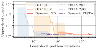
(a) Objective value $f(\theta)$

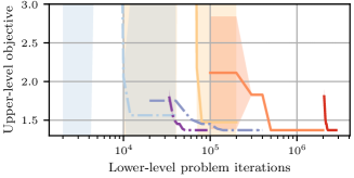
(b) Objective value $f(\theta)$, zoomed in

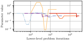
(c) Parameter value $\alpha_{\theta}$

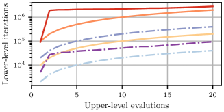
(d) Cumulative GD/FISTA iterations per upper-level evaluation

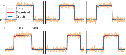
Figure 4: Results for the 1-parameter denoising problem.

Figure 5: 1-parameter final reconstructions (dynamic accuracy FISTA but all except low-accuracy GD look basically the same). Reconstructions are calculated by using the final $\theta$ returned from the given DFO-LS variant, and solving (6) with 1,000 iterations of FISTA.

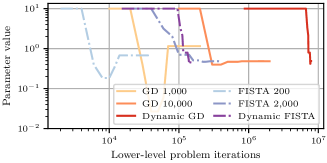
(a) Start $\theta^{0}=1$

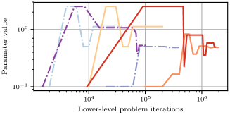
(b) Start $\theta^{0}=-1$

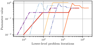
(c) Start $\theta^{0}=-2$

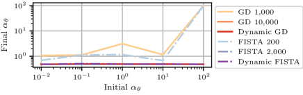
Figure 6: 1-parameter results: optimal $\alpha_{\theta}$ found when using different initial values $\theta^{0}$ (compare Figure 4c).

Figure 7: 1-parameter results: compare optimal $\alpha_{\theta}$ values found for different choices of starting points.

We see that both low-accuracy variants do not converge to the optimal $\theta$. Both high-accuracy variants converge to the same objective value and $\theta$, but take much more computational effort to do this. Indeed, we did not know a priori how many GD/FISTA iterations would be required to achieve convergence. By contrast, both dynamic accuracy variants find the optimal $\theta$ without any tuning.

Moreover, dynamic accuracy FISTA converges faster than high-accuracy FISTA, but the reverse is true for GD. In Figure 4d we show the cumulative number of GD/FISTA iterations performed after each evaluation of the upper-level objective. We see that the reason for dynamic accuracy GD converging slower than than high-accuracy GD is that the initial upper-level evaluations require many GD iterations; the same behavior is seen in dynamic accuracy FISTA, but to a lesser degree. This behavior is entirely determined by our (arbitrary) choices of $\theta^{0}$ and $\Delta^{0}$. We also note that the number of GD/FISTA iterations required by the dynamic accuracy variants after the initial phase is much lower than both the fixed accuracy variants. The difference between the GD and FISTA behavior in Figure 4d is based on how the initial dynamic accuracy requirements compares to the chosen number of high-accuracy iterations (10,000 GD or 2,000 FISTA). Finally, in Figure 5 we show the reconstructions achieved using the $\alpha_{\theta}$ found by dynamic accuracy FISTA. All reconstructions are close to the ground truth, with a small loss of contrast.

To further understand the impact of the initial evaluations and the robustness of our framework, in Figure 5 we run the same problem with different choices $\theta^{0}\in\{-2,-1,1\}$ (where $\theta^{0}=0$ before). In Figure 7 we show best $\alpha_{\theta}$ found for a given computational effort for these choices. When $\theta^{0}>0$, the lower-level problem is starts more ill-conditioned, and so the first upper-level evaluations for the dynamic accuracy variants require more GD/FISTA iterations. However, when $\theta^{0}<0$, we initially have a well-conditioned lower-level problem, and so the dynamic accuracy variants require many fewer GD/FISTA iterations initially, and they converge at the same or a faster rate than the high-accuracy variants.

These results also demonstrate that the dynamic accuracy variants give a final regularization parameter which is robust to the choice of $\theta^{0}$. In Figure 7 we plot the final learned $\alpha_{\theta}$ value compared to the initial choice of $\alpha_{\theta}$ for all variants. The low-accuracy variants do not reach a consistent minimizer for different starting values, but the dynamic and high-accuracy variants both reach the same minimizer for all starting points. Thus although our upper-level problem is nonconvex, we see that our dynamic accuracy approach can produce solutions which are robust to the choice of starting point.

3-parameter denoising results

Next, we consider the 3-parameter ($\alpha_{\theta}$, $\nu_{\theta}$ and $\xi_{\theta}$) denoising problem.

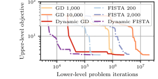
(a) Objective value $f(\theta)$

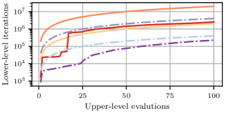
(b) Cumulative GD/FISTA iterations per upper-level evaluation

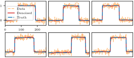
Figure 8: Results for the 3-parameter 1D denoising problem.

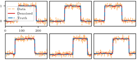
Figure 9: Example 3-parameter final reconstructions (dynamic accuracy FISTA but all other variants are similar). Reconstructions use the final $\theta$ returned by DFO-LS and solving (6) with 1,000 FISTA iterations.

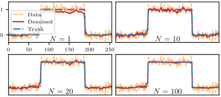
Figure 10: Example 3-parameter final reconstructions for dynamic accuracy FISTA with $\beta=10^{-4}$. Compare with reconstructions with $\beta=10^{-6}$ shown in Figure 11.

Figure 11: 3-parameter results (dynamic accuracy FISTA): reconstructions of first training image using best parameters $\theta$ after $N$ evaluations of upper-level objective (reconstruction based on 1,000 FISTA iterations).

As shown in Figure 11, both dynamic accuracy variants (GD and FISTA) achieve the best objective value at least one order of magnitude faster than the corresponding low- and high-accuracy variants. We note that (for instance) 200 FISTA iterations was insufficient to achieve convergence in the 1-parameter case, but converges here. By contrast, aside from the substantial speedup in the 3-parameter case, our approach converges in both cases without needing to select the computational effort in advance.

The final reconstructions achieved by the optimal parameters for dynamic accuracy FISTA are shown in Figure 11. We note that all variants produced very similar reconstructions (since they converged to similar parameter values), and that all training images are recovered with high accuracy.

Next, we consider the effect of the upper-level regularization parameter $\beta$. If the smaller $\beta$ value of $10^{-8}$ is chosen, all variants converge to slightly smaller values of $\nu_{\theta}$ and $\xi_{\theta}$ as the original $\beta=10^{-6}$, but produce reconstructions of a similar quality. However, increasing the value of $\beta$ yields parameters which give noticeably worse reconstructions. The reconstructions for $\beta=10^{-4}$ are shown in Figure 11.

We conclude by demonstrating in Figure 11 that, aside from reducing our upper-level objective , the parameters found by DFO-LS do in fact progressively improve the quality of the reconstructions. The figure shows the reconstructions of one training image achieved by the best parameters found (by the dynamic accuracy FISTA variant) after a given number of upper-level objective evaluations. We see a clear improvement in the quality of the reconstruction as the upper-level optimization progresses.

4.3 Application: 2D denoising

Next, we demonstrate the performance of dynamic accuracy DFO-LS on the same 3-parameter denoising problem from Section 4.2, but applied to 2D images. Our training data are the 25 images from the Kodak dataset. We select the central $256\times 256$-pixel region of each image, convert to monochrome and add Gaussian noise $N(0,\sigma^{2})$ with $\sigma=0.1$ to each pixel independently. We run DFO-LS for 200 upper-level evaluations with $\rho_{\rm end}=10^{-6}$. Unlike Section 4.2, we find that there is no need to regularize the upper-level problem with the condition number of the lower-level problem (i.e. $\mathcal{J}(\theta)=0$ for these results).

The resulting objective decrease, final parameter values and cumulative lower-level iterations are shown in Figure 12. All variants achieve the same (upper-level) objective value and parameter $\alpha_{\theta}$, but the dynamic accuracy variants achieve this with substantially fewer GD/FISTA iterations compared to the low- and high-accuracy variants. Interestingly, despite all variants achieving the same upper-level objective value, they do not reach a consistent choice for $\nu_{\theta}$ and $\xi_{\theta}$.

In Figure 14 we show the reconstructions achieved by the dynamic accuracy FISTA variant for three of the training images. We see high-quality reconstructions in each case, where the piecewise-constant reconstructions favored by TV regularization are evident.

Lastly, we study the impact of changing the noise level $\sigma$ on the calibrated total variational regularization parameter $\alpha_{\theta}$. We run DFO-LS with dynamic accuracy FISTA for 200 upper-level evaluations on the same training data, but corrupted with noise level $\sigma$ ranging from $10^{-1}$ (as above) to $10^{-8}$, see Figure 14. We see that as $\sigma\to 0$, so does $\alpha_{\theta}$ and $\sigma^{2}/\alpha_{\theta}$. Note that this is a common assumption on the parameter choice rule in regularization theory to yield a convergent regularization method Scherzer2008book (5, 1). It is remarkable that the learned optimal parameter also has this property.

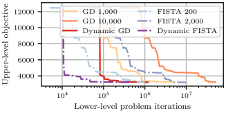
(a) Objective value $f(\theta)$

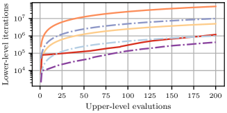
(b) Cumulative GD/FISTA iterations per upper-level evaluation

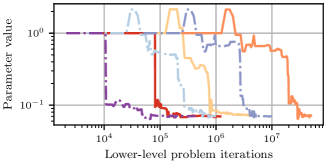
(c) Parameter value $\alpha_{\theta}$

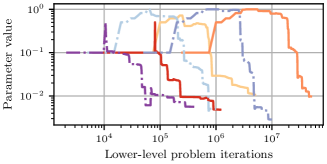
(d) Parameter value $\nu_{\theta}$

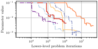
(e) Parameter value $\xi_{\theta}$

Figure 12: Results for the 3-parameter denoising problem with 2D images.

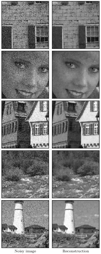
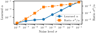
Figure 13: Example reconstructions using denoising parameters (dynamic FISTA DFO-LS variant). Reconstructions generated with 2,000 FISTA iterations of the lower-level problem.

Figure 14: Learned regularization parameter $\alpha_{\theta}$ for 2D TV-denoising with varying noise levels $\sigma$.

4.4 Application: Learning MRI Sampling Patterns

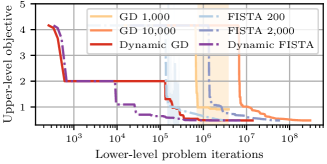
(a) Objective value $f(\theta)$

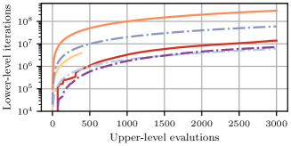
(b) Cumulative GD/FISTA iterations per upper-level evaluation

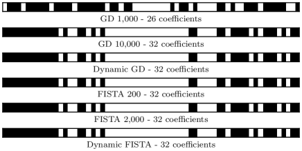
Figure 15: Results for the MRI sampling problem. Note: the low-accuracy GD variant ($K=1,000$) terminates on a small trust-region radius, as it is unable to make further progress.

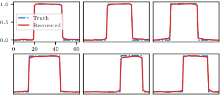
Figure 16: Final (after thresholding) MRI sampling patterns found by each DFO-LS variant. This only shows which Fourier coefficients have $\theta_{i}>0.001$, it does not show the relative magnitudes of each $\theta_{i}$.

Figure 17: Reconstructions using final (after thresholding) MRI sampling pattern found by the dynamic FISTA variant of DFO-LS. Results from running 2,000 FISTA iterations of the lower-level problem.

Lastly, we turn our attention to the problem of learning MRI sampling patterns. In this case, our lower-level problem is (6) with $A(\theta)=F$, where $F$ is the Fourier transform, and $S(\theta)$ is a nonnegative diagonal sampling matrix. Following Chen2014 (33), we aim to find sampling parameters $\theta\in[0,1]^{d}$ corresponding to the weight associated to each Fourier mode, our sampling matrix is defined as

$$S(\theta):=\operatorname{diag}\left(\frac{\theta_{1}}{1-\theta_{1}},\ldots,\frac{\theta_{d}}{1-\theta_{d}}\right)\in\mathbb{R}^{d\times d}.$$ (87)

The resulting lower-level problem is $\mu$-strongly convex and $L$-smooth as per (7) with $\|A_{\theta}^{*}S_{\theta}A_{\theta}\|=\|S(\theta)\|=\max_{i}\theta_{i}/(1-\theta_{i})$ and $\lambda_{\operatorname{min}}(A_{\theta}^{*}S_{\theta}A_{\theta})=\min_{i}\theta_{i}/(1-\theta_{i})$.

For our testing, we fix the regularization and smoothness parameters $\alpha=0.01$, $\nu=0.01$ and $\xi=10^{-4}$ in (6). We use $n=10$ training images constructed using the method described in Section 2.2 with $N=64$ and $\sigma=0.05$. Lastly, we add a penalty to our upper-level objective to encourage sparse sampling patterns: $\mathcal{J}(\theta):=\beta\|\theta\|_{1}$, where we take $\beta=0.1$. To fit the least-squares structure (22), we rewrite this term as $\mathcal{J}(\theta)=(\sqrt{\beta\|\theta\|_{1}})^{2}$. To ensure that $S(\theta)$ remains finite and $\mathcal{J}(\theta)$ remains $L$-smooth, we restrict $0.001\leq\theta_{i}\leq 0.99$.

We run DFO-LS with a budget of 3000 evaluations of the upper-level objective and $\rho_{\rm end}=10^{-6}$. As in Section 4.2, we compare dynamic accuracy DFO-LS against (fixed accuracy) DFO-LS with low- and high-accuracy evaluations given by a 1,000 and 10,000 iterations of GD or 200 and 1,000 iterations of FISTA.

With our $\ell_{1}$ penalty on $\theta$, we expect DFO-LS to find a solution where many entries of $\theta$ are at their lower bound $\theta_{i}=0.001$. Our final sampling pattern is chosen by using the corresponding $\theta_{i}$ if $\theta_{i}>0.001$, otherwise we set that Fourier mode weight to zero.

In Figure 17 we show the objective decrease achieved by each variant, and the cumulative lower-level work required by each variant. All variants except low-accuracy GD achieve the best objective value with low uncertainty. However, as above, the dynamic accuracy variants achieve this value significantly earlier than the fixed accuracy variants, largely as a result of needing much fewer GD/FISTA iterations in the (lower accuracy) early upper-level evaluations. In particular dynamic accuracy GD reaches the minimum objective value about 100 times faster than high-accuracy GD. We note that FISTA with 200 iterations ends up requiring fewer lower-level iterations after a large number of upper-level evaluations, but the dynamic accuracy variant achieves is minimum objective value sooner.

We show the final pattern of sampled Fourier coefficients (after thresholding) in Figure 17. Of the five variants which found the best objective value, all reached a similar set of ‘active’ coefficients $\theta_{i}>0.001$ with broadly similar values for $\theta_{i}$ at all frequencies. For demonstration purposes we plot the reconstructions corresponding to the coefficients from the ‘dynamic FISTA’ variant in Figure 17 (the reconstructions of the other variants were all similar). All the training images are reconstructed to high accuracy, with only a small loss of contrast near the jumps.

5 Conclusion

We introduce a dynamic accuracy model-based DFO algorithm for solving bilevel learning problems. This approach allows us to learn potentially large numbers of parameters, and allowing inexact upper-level objective evaluations with which we dramatically reduce the lower-level computational effort required, particularly in the early phases of the algorithm. Compared to fixed accuracy DFO methods, we often achieve better upper-level objective values and low-accuracy methods, and similar objective values as high-accuracy methods but with much less work: in some cases up to 100 times faster. These observations can be made for both lower-level solvers GD and FISTA, with different fixed accuracy requirements, for ROF-denoising and learning MRI sampling patterns. Thus the proposed approach is robust in practice, computationally efficient and backed by convergence and worst-case complexity guarantees. Although the upper-level problem is nonconvex, our numerics do not suggest that convergence to non-global minima is a point for concern here.

Future work in this area includes relaxing the smoothness and/or strong convexity assumptions on the lower-level problem (making the upper-level problem less theoretically tractable). Our theoretical analysis would benefit from a full proof that our worst-case complexity bound on the lower-level computational work is tight. Another approach for tackling bilevel learning problems would be to consider gradient-based methods which allow inexact gradient information. Lastly, bilevel learning appears to compute a regularization parameter choice strategy which yields a convergent regularization method. Further investigation is required to back these numerical results by sound mathematical theory.

References

- (1) Kazufumi Ito and Bangti Jin “Inverse Problems - Tikhonov Theory and Algorithms” World Scientific Publishing, 2014 DOI: 10.1142/9120
- (2) Martin Benning and Martin Burger “Modern regularization methods for inverse problems” In Acta Numerica 27, 2018, pp. 1–111 DOI: 10.1017/S0962492918000016
- (3) Antonin Chambolle and Thomas Pock “An Introduction to Continuous Optimization for Imaging” In Acta Numerica 25, 2016, pp. 161–319 DOI: 10.1017/S096249291600009X
- (4) Simon Arridge, Peter Maass, Ozan Öktem and Carola-Bibiane Schönlieb “Solving inverse problems using data-driven models” In Acta Numerica 28, 2019, pp. 1–174 DOI: 10.1017/S0962492919000059
- (5) Otmar Scherzer et al. “Variational Methods in Imaging”, 2008
- (6) H.. Engl, M. Hanke and A. Neubauer “Regularization of Inverse Problems”, Mathematics and Its Applications Springer, 1996
- (7) Per Christian Hansen “Analysis of Discrete Ill-Posed Problems by Means of the L-Curve” In SIAM Review 34.4, 1992, pp. 561–580 DOI: 10.1137/1034115
- (8) Kristian Bredies, Karl Kunisch and Thomas Pock “Total Generalized Variation” In SIAM Journal on Imaging Sciences 3.3, 2010, pp. 492–526 DOI: 10.1137/090769521
- (9) Muhammad Usman and Philip G Batchelor “Optimized Sampling Patterns for Practical Compressed MRI” In International Conference on Sampling Theory and Applications, 2009
- (10) Baran Gözcü et al. “Learning-Based Compressive MRI” In IEEE Transactions on Medical Imaging 37.6, 2018, pp. 1394–1406 DOI: 10.1109/TMI.2018.2832540
- (11) Ferdia Sherry et al. “Learning the Sampling Pattern for MRI” In IEEE Transactions on Medical Imaging 39.12, 2020, pp. 4310–4321
- (12) Juan Carlos De Los Reyes and Carola-Bibiane Schönlieb “Image Denoising: Learning the Noise Model via Nonsmooth PDE-Constrained Optimization” In Inverse Problems and Imaging 7, 2013, pp. 1183–1214
- (13) Karl Kunisch and Thomas Pock “A Bilevel Optimization Approach for Parameter Learning in Variational Models” In SIAM Journal on Imaging Sciences 6.2, 2013, pp. 938–983 DOI: 10.1137/120882706
- (14) Peter Ochs, René Ranftl, Thomas Brox and Thomas Pock “Bilevel Optimization with Nonsmooth Lower Level Problems” In SSVM 9087, 2015, pp. 654–665 DOI: 10.1007/978-3-319-18461-6
- (15) Michael Hintermüller, Kostas Papafitsoros, Carlos N. Rautenberg and Hongpeng Sun “Dualization and Automatic Distributed Parameter Selection of Total Generalized Variation via Bilevel Optimization”, 2020 arXiv: http://arxiv.org/abs/2002.05614
- (16) Erlend S. Riis, Matthias J. Ehrhardt, G… Quispel and Carola-Bibiane Schönlieb “A geometric integration approach to nonsmooth, nonconvex optimisation”, 2018 arXiv: http://arxiv.org/abs/1807.07554
- (17) S oren Bartels and Nico Weber “Parameter learning and fractional differential operators: application in image regularization and decomposition”, 2020 arXiv: https://arxiv.org/abs/2001.03394
- (18) Andrew R. Conn, Katya Scheinberg and Luís N. Vicente “Introduction to Derivative-Free Optimization” 8, MPS-SIAM Series on Optimization Philadelphia: MPS/SIAM, 2009 DOI: 10.1137/1.9780898718768
- (19) Charles Audet and Warren Hare “Derivative-Free and Blackbox Optimization”, Springer Series in Operations Research and Financial Engineering Cham, Switzerland: Springer, 2017 DOI: 10.1007/978-3-319-68913-5
- (20) Jeffrey W. Larson, Matt Menickelly and Stefan M. Wild “Derivative-free optimization methods” In Acta Numerica 28, 2019, pp. 287–404 DOI: 10.1017/S0962492919000060
- (21) Charles Audet and Dominique Orban “Finding optimal algorithmic parameters using derivative-free optimization” In SIAM Journal on Optimization 17.3, 2006, pp. 642–664 DOI: 10.1137/040620886
- (22) Dounia Lakhmiri, Sébastien Le Digabel and Christophe Tribes “HyperNOMAD: Hyperparameter optimization of deep neural networks using mesh adaptive direct search”, 2019 arXiv: https://arxiv.org/abs/1907.01698
- (23) Hongchao Zhang, Andrew R. Conn and Katya Scheinberg “A Derivative-Free Algorithm for Least-Squares Minimization” In SIAM Journal on Optimization 20.6, 2010, pp. 3555–3576 DOI: 10.1137/09075531X
- (24) Coralia Cartis and Lindon Roberts “A derivative-free Gauss-Newton method” In Mathematical Programming Computation 11.4, 2019, pp. 631–674 DOI: 10.1007/s12532-019-00161-7
- (25) Andrew R. Conn and Luís N. Vicente “Bilevel derivative-free optimization and its application to robust optimization” In Optimization Methods and Software 27.3, 2012, pp. 561–577 DOI: 10.1080/10556788.2010.547579
- (26) Andrew R. Conn, Nicholas I.. Gould and Philippe L. Toint “Trust-Region Methods” 1, MPS-SIAM Series on Optimization Philadelphia: MPS/SIAM, 2000 DOI: 10.1137/1.9780898719857
- (27) Ruobing Chen, Katya Scheinberg and Brian Y. Chen “Aligning Ligand Binding Cavities by Optimizing Superposed Volume” In 2012 IEEE International Conference on Bioinformatics and Biomedicine, 2012 DOI: 10.1109/BIBM.2012.6392629
- (28) Stefania Bellavia, Gianmarco Gurioli, Benedetta Morini and Philippe L. Toint “Adaptive Regularization Algorithms with Inexact Evaluations for Nonconvex Optimization”, 2019 arXiv: https://arxiv.org/abs/1811.03831
- (29) S. Gratton, E. Simon and Ph.. Toint “Minimization of nonsmooth nonconvex functions using inexact evaluations and its worst-case complexity”, 2019 arXiv: https://arxiv.org/abs/1902.10406
- (30) Andrew March and Karen Willcox “Provably convergent multifidelity optimization algorithm not requiring high-fidelity derivatives” In AIAA Journal 50.5, 2012, pp. 1079–1089 DOI: 10.2514/1.J051125
- (31) Henri Calandra, Serge Gratton, Elisa Riccietti and Xavier Vasseur “On high-order multilevel optimization strategies”, 2019 arXiv: https://arxiv.org/abs/1904.04692
- (32) Clément W. Royer, Michael O’Neill and Stephen J. Wright “A Newton-CG Algorithm with Complexity Guarantees for Smooth Unconstrained Optimization” In Mathematical Programming 180.1-2, 2020, pp. 451–488
- (33) Yunjin Chen, René Ranftl, Thomas Brox and Thomas Pock “A bi-level view of inpainting-based image compression” In 19th Computer Vision Winter Workshop, 2014
- (34) R. Rockafellar and Roger J-B Wets “Variational analysis” In Variational Analysis, 2008 DOI: 10.1021/jp7118845
- (35) Kristian Bredies and Dirk A Lorenz “Mathematical Image Processing” Birkhäuser Basel, 2018 DOI: 10.1007/978-3-030-01458-2
- (36) Stephen M Robinson “Strongly Regular Generalized Equations” In Mathematics of Operations Research 5.1, 1980, pp. 43–62
- (37) J J Duistermaat and J A C Kolk “Multidimensional Real Analysis I: Differentiation” New York: Cambridge University Press, 2004
- (38) Leonid I Rudin, Stanley Osher and Emad Fatemi “Nonlinear Total Variation based Noise Removal Algorithms” In Physica D: Nonlinear Phenomena 60.1 Elsevier, 1992, pp. 259–268 DOI: 10.1016/0167-2789(92)90242-F
- (39) Michael Lustig, David L. Donoho and John M. Pauly “Sparse MRI: The Application of Compressed Sensing for Rapid MR Imaging” In Magnetic Resonance in Medicine 58.6, 2007, pp. 1182–1195 DOI: 10.1002/mrm.21391
- (40) Amir Beck “First-Order Methods in Optimization” 25, MOS-SIAM Series on Optimization Philadelphia: MOS/SIAM, 2017
- (41) Yurii Nesterov “Introductory Lectures on Convex Optimization: A Basic Course” Dordrecht, Netherlands: Kluwer Academic Publishers, 2004
- (42) Amir Beck and Marc Teboulle “A Fast Iterative Shrinkage-Thresholding Algorithm” In SIAM Journal on Imaging Sciences 2.1, 2009, pp. 183–202 DOI: 10.1137/080716542
- (43) Yurii Nesterov “A method for solving the convex programming problem with convergence rate ” In Doklady Akademii Nauk SSSR 269.3, 1983, pp. 543–547
- (44) Jorge Nocedal and Stephen J. Wright “Numerical Optimization”, Springer Series in Operations Research and Financial Engineering New York: Springer, 2006 DOI: 10.1007/978-0-387-40065-5
- (45) R. Garmanjani, Diogo Júdice and Luís N. Vicente “Trust-Region Methods Without Using Derivatives: Worst Case Complexity and the Nonsmooth Case” In SIAM Journal on Optimization 26.4, 2016, pp. 1987–2011 DOI: 10.1137/151005683
- (46) J.C. De Los Reyes, C.-B. Schönlieb and T. Valkonen “The Structure of Optimal Parameters for Image Restoration Problems”, 2016, pp. 464–500
- (47) Coralia Cartis, Jan Fiala, Benjamin Marteau and Lindon Roberts “Improving the Flexibility and Robustness of Model-Based Derivative-Free Optimization Solvers” In ACM Transactions on Mathematical Software 45.3, 2019, pp. 32:1–32:41 DOI: 10.1145/3338517