Spectral Evolution with Approximated Eigenvalue Trajectories for Link Prediction

Abstract

The spectral evolution model aims to characterize the growth of large networks (i.e., how they evolve as new edges are established) in terms of the eigenvalue decomposition of the adjacency matrices. It assumes that, while eigenvectors remain constant, eigenvalues evolve in a predictable manner over time. This paper extends the original formulation of the model twofold. First, it presents a method to compute an approximation of the spectral evolution of eigenvalues based on the Rayleigh quotient. Second, it proposes an algorithm to estimate the evolution of eigenvalues by extrapolating only a fraction of their approximated values. The proposed model is used to characterize mention networks of users who posted tweets that include the most popular political hashtags in Colombia from August $2017$ to August $2018$ (the period which concludes the disarmament of the Revolutionary Armed Forces of Colombia). To evaluate the extent to which the spectral evolution model resembles these networks, link prediction methods based on learning algorithms (i.e., extrapolation and regression) and graph kernels are implemented. Experimental results show that the learning algorithms deployed on the approximated trajectories outperform the usual kernel and extrapolation methods at predicting the formation of new edges.

1 Introduction

Many systems of interest have the form of a network (or graph) where entities are represented as nodes and relationships between pairs of nodes as edges. Modeling and analyzing these networks tend to become more complex as they grow in size (both in terms of nodes and edges) and in the number of concurrent processes (activities that occur at the same time across different nodes). Not surprisingly, efforts to explain the tangled dynamics of empirical networks of overwhelming size have received increasing attention in recent years. Numerous approaches have been proposed to gain a better understanding of network behavior. For example, the detection of malicious accounts in location-based social networks is a first step to provide reliable information to users and improve their user experiences (Gong et al., 2018). Predicting the relationships of online social networks has been key in identifying whether influential users maintain their status, or whether a political polarization of a group of nodes reflects a transitory or stationary state (DiMaggio et al., 1996). Similarly, information of users across different social platforms has been used to develop a multi-layer algorithm that predicts links on social networks (Jalili et al., 2017). Modeling Twitter data as a co-occurrence language network has also been used to infer future relationships between users (Martinčić-Ipšić et al., 2017). In all these studies, a common goal is to develop models that capture node interactions and predict how new edges are established over time.

The field of  spectral graph theory is one of the fundamental pillars for the study of networks (Godsil & Royle, 2001). It uses eigenvalues and eigenvectors of matrices associated with graphs to shed light and reveal combinatorial properties of networks (Kurucz et al., 2009). Common associations include the adjacency and Laplacian matrices, which range over the nodes of the graph and may be symmetric or asymmetric. In either case, such matrices can be viewed both as an operator mapping vectors to vectors and as a mean to define quadratic forms. Any real-valued symmetric matrix $\mathbf{A}$ with $n$ rows (and columns) can be characterized by its spectral decomposition, i.e., a set of pairs of eigenvalues and eigenvectors $(\mathbf{X},\Lambda)=\{(\mathbf{x_{1}},\lambda_{1}),\ldots,(\mathbf{x_{n}},\lambda_{n})\}$ such that the equation $\mathbf{A}\mathbf{x_{i}}=\lambda_{i}\mathbf{x_{i}}$ holds for each $1\leq i\leq n$. Therefore, the evolution of a graph with $n$ vertices can be represented either by a sequence $\mathbf{A}_{1},\ldots,\mathbf{A}_{t}$ of symmetric $n\times n$ matrices or by a sequence of their spectral decompositions $(\mathbf{X}_{1},\Lambda_{1}),\ldots,(\mathbf{X}_{t},\Lambda_{t})$. From a practical viewpoint, spectral decomposition becomes a powerful tool to predict, under certain assumptions on how each pair of eigenvalues and eigenvectors behaves, the evolution of networks.

In particular, the spectral evolution model (Kunegis et al., 2013) characterizes the dynamics of a network (i.e., how new edges are created over time) in terms of the evolution of its spectra, assuming that the associated eigenvectors remain largely constant. That is, within the spectral evolution model framework, each sequence of symmetric matrices $\mathbf{A}_{1},\ldots,\mathbf{A}_{t}$ is characterized solely by the set of eigenvectors, say $\mathbf{X}_{t}$, and the spectra $\Lambda_{1},\ldots,\Lambda_{t}$. By neglecting possible minor changes in the behavior of the eigenvectors, efforts to characterize the dynamics of a network focus exclusively on predicting the trajectory of the eigenvalues.

This paper extends the original spectral evolution model (Kunegis et al., 2013) by introducing a tandem of two techniques that complement each other. First, the extended model predicts how a network grows based on extrapolating an approximation of its eigenvalues. Common kernel and extrapolation methods are memoryless in the sense that only one or two network snapshots are considered for extrapolating eigenvalues. In other words, the evolution history of the network is mostly neglected. The working hypothesis is that, by considering an entire sequence of eigenvalue approximations $\hat{\Lambda}_{1},\ldots,\hat{\Lambda}_{t}$, better eigenvalue trajectories may be computed to predict links at time $t+1$. Each approximation $\hat{\Lambda}_{i}$ is computed by using the Rayleigh quotient (Chatelin, 2012) and extrapolation can be achieved by fitting the trajectory of the approximated eigenvalues with regression algorithms. The resulting approach to compute $\mathbf{A}_{t+1}$ takes $O(tn^{3})$ time, which is asymptotically equivalent to checking the extended model hypothesis on the sequence $\mathbf{A}_{1},\ldots,\mathbf{A}_{t}$ with state-of-the-art algorithms. In practice, this means that the proposed approach can always be used as an extension of the spectral evolution model, without adding significant computational costs.

The second contribution is based on an experimental observation: The learning algorithms can accurately predict the evolution of the eigenvalues by only taking into account a fraction of all the approximated trajectories. That is, instead of working with the $n$ eigenvalue trajectories to compute $\mathbf{A}_{t+1}$, it is sufficient to consider a fraction of the trajectories in order to achieve an accurate link prediction. Therefore, the above-mentioned computational effort can be reduced further in practice by a constant factor. For instance, in some experiments, the adjacency matrix $\mathbf{A}_{t+1}$ can be recovered with an accuracy of $99.97\%$ when only $8\%$ of the trajectories are considered.

The proposed approach is used to explain the evolution networks of Twitter users who posted messages with political hashtags. In these networks, each node represents a user. An edge is present between two users (nodes) whenever any of the two users mentions the other in a message containing a selected hashtag. The selection corresponds to the most popular hashtags associated to political affairs in Colombia between August $2017$ and August $2018$. This period marks the disarmament of the Revolutionary Armed Forces of Colombia (Farc) and the end of an armed conflict that lasted over 50 years (Ince, 2013; Saab & Taylor, 2009). The experimental exploration suggests that spectral extrapolation methods based on linear and quadratic regression outperform the approaches based on graph kernels. Achieving a better performance is related to the ability to capture the irregular evolution of the eigenvalues (i.e., for scenarios in which the rate of growth of some eigenvalues is higher than for others).

Finally, it is important to note that this paper builds on results presented in (Romero et al., 2020). Unlike the work in (Romero et al., 2020), the model presented here is equipped with the Raleigh quotient for computing approximated spectra. Furthermore, new learning algorithms have been evaluated to predict the trajectories of the eigenvalues. Finally, unlike (Romero et al., 2020), the mention networks are not considered multi-graphs but simple graphs, which renders edge prediction into a binary classification problem.

Outline. The remainder of the paper is organized as follows. Section 2 presents the spectral evolution model. Section 3 introduces the extended spectral evolution model, including the Rayleigh quotient and the approximation of spectral trajectories. Section 4 describes the mention networks used for the experimental analysis and presents the results of applying the proposed approach to these networks. Section 5 draws some concluding remarks and future research directions.

2 Preliminaries

This section presents preliminaries on the spectral evolution model, including common growth methods based on graph kernels and spectral extrapolation used for link prediction. The overview is, mainly, based on (Kunegis et al., 2013).

2.1 Spectral Representation

A graph $G=(V,E)$ is specified by its vertex set $V$ and its edge set $E$; throughout the rest of paper it is assumed that any graph is finite (i.e., $|V|$ is a natural number), undirected, and without self or multiple edges. Without loss of generality, the vertex set $V$ is assumed to be ordered, e.g., $V=\{1,2,3,\ldots,|V|\}$. To any graph $G=(V,E)$ a matrix $\mathbf{A}_{G}$ (or simply $\mathbf{A}$) is associated whose entries are given for any $u,v\in V$ by $\mathbf{A}(u,v)=1$ if $(u,v)\in E$ and $\mathbf{A}(u,v)=0$ if $(u,v)\notin E$. The matrix $\mathbf{A}$ is called the adjacency matrix of $G$. Under the above assumptions, any adjacency matrix is symmetric.

A vector $\mathbf{x}$ is an eigenvector of a matrix $\mathbf{A}$ with eigenvalue $\lambda$ iff $\mathbf{A}\mathbf{x}=\lambda\mathbf{x}$. The spectral theorem states an important fact about symmetric adjacency matrices.

Theorem 2.1

Let $n\in\mathbb{N}$ be positive. If $\mathbf{A}$ is a $n$-by-$n$ symmetric matrix, with real entries, then there exist real numbers $\lambda_{1},\lambda_{2},\ldots,\lambda_{n}$ and $n$ mutually orthogonal unit vectors $\mathbf{x}_{1},\mathbf{x}_{2},\ldots,\mathbf{x}_{n}$ such that $\mathbf{x}_{i}$ is an eigenvector of $\mathbf{A}$ with eigenvalue $\lambda_{i}$, for $1\leq i\leq n$.

The pair $(\mathbf{X},\mathbf{\Lambda})$, with $\mathbf{X}$ being the orthogonal matrix obtained from the unit vectors $\mathbf{x}_{1},\ldots,\mathbf{x}_{n}$ and $\mathbf{\Lambda}$ the diagonal matrix determined by $\lambda_{1},\ldots,\lambda_{n}$ in Theorem 2.1, is called the spectral decomposition of $\mathbf{A}$ and satisfies $\mathbf{A}=\mathbf{X}\mathbf{\Lambda}\mathbf{X}^{T}$. It is important to note that eigenvalues are uniquely determined, but can be repeated. However, eigenvectors are not uniquely determined for a given eigenvalue. In general, the eigenvectors of a given eigenvalue are determined modulo orthogonal transformations.

2.2 The Spectral Evolution Model

The spectral evolution model (Kunegis et al., 2013) assumes that the evolution of a network can be described by the evolution in the network’s spectrum, while the networks eigenvectors stay largely constant over time. Formally, if $\mathbf{A}_{t}$ is the adjacency matrix of a network at time $t$ and $(\mathbf{X}_{t},\mathbf{\Lambda}_{t})$ its spectral decomposition, then the spectral decomposition $(\mathbf{X}_{t^{\prime}},\mathbf{\Lambda}_{t^{\prime}})$ of the adjacency matrix of the network at any time $t^{\prime}$ satisfies $\mathbf{X}_{t}\approx\mathbf{X}_{t^{\prime}}$ (i.e., the eigenvectors of $\mathbf{A}_{t}$ and $\mathbf{A}_{t^{\prime}}$ are approximately the same over time).

There are, basically, two existing approaches to link prediction with the spectral evolution model: spectral transformation functions (based on graph kernels) and spectral extrapolation.

2.2.1 Spectral Transformation

Link prediction can be expressed as a spectral decomposition $\mathbf{X}F(\mathbf{\Lambda})\mathbf{X}^{T}$, where $F$ is a spectral transformation that applies the same real function to each diagonal element $\lambda_{j}$ of $\mathbf{\Lambda}$.

The Triangle Closing Kernel. The triangle closing kernel is expressed as $\mathbf{A}^{2}=\mathbf{X}\mathbf{\Lambda}^{2}\mathbf{X}^{T}$. That is, the kernel replaces the eigenvalues of $\mathbf{A}$ by their squared values. The function associated to the triangle closing kernel is $f(\lambda)=\lambda^{2}$.

Exponential Kernel. The exponential kernel is expressed as

$$\exp{(\alpha\mathbf{A})}=\sum_{k=0}^{\infty}\alpha^{k}\frac{1}{k!}\mathbf{A}^{k},$$

where $\alpha$ is a constant used to balance the weight of short and long paths. It denotes the sum of every path between two vertices weighted by the inverse factorial of its length. The function associated to the exponential kernel is $f(\lambda)=e^{\alpha\lambda}$.

Neumann Kernel. The Neumann kernel is expressed as

$$(\mathbf{I}-\alpha\mathbf{A})^{-1}=\sum_{k=0}^{\infty}\alpha^{k}\mathbf{A}^{k},$$

where $\alpha^{-1}>|\lambda_{1}|$ and $\lambda_{1}$ is the largest eigenvalue of $\mathbf{A}$. The function associated to the Neumann kernel is $f(\lambda)=1/(1-\alpha\lambda)$.

2.2.2 Spectral Extrapolation

Graph kernels can characterize a spectral transformation function for the growth of the spectrum. However, when the evolution of the spectrum is irregular, it is not always possible to find a simple function that describes the trajectory for all eigenvalues. In this situation, it is often convenient to use spectral extrapolation, which can be viewed as a generalization of graph kernels.

Let $t_{1}$ be an intermediate time and $t_{2}$ the final time from which link prediction is to be made, and let $\mathbf{A}_{1}$ and $\mathbf{A}_{2}$ be the adjacency matrices of the network at times $t_{1}$ and $t_{2}$, respectively. These matrices can be decomposed as $\mathbf{A}_{1}=\mathbf{X}_{1}\mathbf{\Lambda}_{1}\mathbf{X}_{1}^{T}$ and $\mathbf{A}_{2}=\mathbf{X}_{2}\mathbf{\Lambda}_{2}\mathbf{X}_{2}^{T}$, for some $\mathbf{X}_{1},\mathbf{\Lambda}_{1},\mathbf{X}_{2},\mathbf{\Lambda}_{2}$. If $(\lambda_{2})_{j}$ is the $j$-th eigenvalue (say, under the ordering of $\mathbf{\Lambda}_{2}$’s diagonal) at $t_{2}$, its estimated previous value $(\hat{\lambda}_{1})_{j}$ at $t_{1}$ is computed as a diagonalization of $\mathbf{A}_{1}$ by $\mathbf{X}_{2}$

$$(\hat{\lambda}_{1})_{j}=\left(\sum_{i}(\mathbf{X}_{1})_{i}^{T}(\mathbf{X}_{2})_{j}\right)^{-1}\sum_{i}(\mathbf{X}_{1}^{T})_{i}(\mathbf{X}_{2})_{j}(\lambda_{1})_{i},$$

where $(\mathbf{X}_{t})_{k}$ is the $k$-th eigenvector for $1\leq k\leq n$, and $(\lambda_{t})_{k}$ is the $k$-th eigenvalue of $\mathbf{A}_{t}$ ($t\in\{1,2\}$), respectively (under the same ordering mentioned above). Note that in this formula, the occurrences of $\mathbf{X}_{1}$ could be replaced by $\mathbf{X}_{2}$ because of the spectral evolution model assumptions. However, if the possible small changes in the eigenvectors are to be taken into account, the given version of the formula should be used.

Linear extrapolation is used to predict link formation in the network at a future time $t_{3}>t_{2}$. The $j$-th eigenvalue at $t_{3}$ is approximated from the eigenvalues $\lambda_{2}$ at time $t_{2}$ and their approximated counter-parts $\hat{\lambda}_{1}$ at time $t_{1}$, as follows:

$$(\hat{\lambda}_{3})_{j}=2(\lambda_{2})_{j}-(\hat{\lambda}_{1})_{j}.$$

Finally, a link prediction real-valued matrix $\hat{\mathbf{A}}_{3}$ is computed as follows:

$$\hat{\mathbf{A}}_{3}=\mathbf{X}_{2}\hat{\mathbf{\Lambda}}_{3}\mathbf{X}_{2}^{T}.$$

Let $\hat{\mathbf{A}}_{3}(u,v)$ denote the entry in row $u$ and column $v$ of $\hat{\mathbf{A}}_{3}$. For each $u,v\in V$, the value $\hat{\mathbf{A}}_{3}(u,v)$ is a link prediction score representing the probability of having at time $t_{3}$ a link between $u$ and $v$. The adjacency matrix $\mathbf{A}_{3}$, which would represent the network at the future time $t_{3}$, can be constructed from $\hat{\mathbf{A}}_{3}$ in many ways. For example, by setting a threshold $0\leq\delta\leq 1$ such that $\mathbf{A}_{3}(u,v)=1$ if $\hat{\mathbf{A}}_{3}(u,v)\geq\delta$ and $\mathbf{A}_{3}(u,v)=0$ if $\hat{\mathbf{A}}_{3}(u,v)<\delta$, for each $u,v\in V$.

3 Extending the Spectral Evolution Model

Consider a network $G$ with $n$ vertices and a sequence of ($n$-by-$n$) adjacency matrices $\mathbf{A}_{1},\mathbf{A}_{2},\ldots,\mathbf{A}_{t}$ representing the evolution of $G$ (i.e., the addition of new edges among existing nodes) over $t$ time units. One or more edges can be created from one time unit to the next. The problem of predicting the formation in $G$ of new edges at time $t+1$ consists in extending the given sequence of adjacency matrices with a new adjacency matrix $\mathbf{A}_{t+1}$. The spectral evolution model introduced in Section 2 can be used for such a task in two ways, under the assumption that the eigenvectors of the adjacency matrices remain constant. On the one hand, a graph kernel can be chosen as a specific spectral transformation function for obtaining $\mathbf{A}_{t+1}$ from $\mathbf{A}_{t}$. On the other hand, a time $t^{\prime}<t$ can be picked so that $\mathbf{A}_{t+1}$ is extrapolated from $\mathbf{A}_{t^{\prime}}$ and $\mathbf{A}_{t}$. In either case, the evolution history of the network $G$ is not fully considered and mostly neglected. The working hypothesis is that, by considering the entire sequence $\mathbf{A}_{1},\mathbf{A}_{2},\ldots,\mathbf{A}_{t}$, better eigenvalue predictions could be computed to build $\mathbf{A}_{t+1}$. That is, the more information about how eigenvalues change over the $t$ time units, the better link prediction for the network would be at time $t+1$. Of course, the key question to ask is how to use all this information and yet have an efficient construction method for $\mathbf{A}_{t+1}$: this section introduces an extrapolation-based approach that answers this question by using approximations computed with the Rayleigh quotient.

3.1 The Rayleigh Quotient

The eigenvalues and eigenvectors of symmetric matrices have many characterizations. The Rayleigh quotient is a tool from linear algebra that offers one of such characterizations (see, e.g.,  (Chatelin, 2012)).

Definition 1

Let $n\in\mathbb{N}$ be positive, $\mathbf{A}$ an (adjacency) $n$-by-$n$ matrix, and $\mathbf{x}$ a real-valued non-zero $n$-vector. The Rayleigh quotient of $\mathbf{x}$ with respect to $\mathbf{A}$ is the ratio $R(\mathbf{A},\mathbf{x})$ defined by

$$R(\mathbf{A},\mathbf{x})=\frac{\mathbf{x}^{T}\mathbf{A}\mathbf{x}}{\mathbf{x}^{T}\mathbf{x}}.$$

Note that the Rayleigh quotient $R(\mathbf{A},\mathbf{x})$ is a real number (i.e., a scalar value). If $\mathbf{x}$ is an eigenvector of $\mathbf{A}$, then the ratio $R(\mathbf{A},\mathbf{x})$ is the corresponding eigenvalue. Also, if a vector $\mathbf{y}$ approximates an eigenvector $\mathbf{x}$ of $\mathbf{A}$, then $R(\mathbf{A},\mathbf{y})$ is an approximation of $R(\mathbf{A},\mathbf{x})$. That is, eigenvalues can be approximated based on approximations of eigenvectors by using the Rayleigh quotient.

3.2 Spectral Extrapolation

Recall the problem of predicting the formation in $G$ of new edges at time $t+1$ from the adjacency matrices $\mathbf{A}_{1},\mathbf{A}_{2},\ldots,\mathbf{A}_{t}$ representing the evolution of $G$ over $t$ time units. The approach is to extrapolate the trajectory of the eigenvalues of the adjacency matrices in this sequence.

Let $(\mathbf{X}_{t},\mathbf{\Lambda}_{t})$ be the spectral decomposition of $\mathbf{A}_{t}$, and let $\mathbf{x}_{j}$ and $\lambda_{j}$ be the $j$-th eigenvector and eigenvalue in $\mathbf{X}_{t}$ and $\mathbf{\Lambda}_{t}$, respectively (i.e., the latent dimension $j$). Under the assumption of the spectral evolution model, the trajectory of $\lambda_{j}$ in $\mathbf{A}_{1},\mathbf{A}_{2},\ldots,\mathbf{A}_{t}$ can be approximated by $\hat{\lambda}_{j}^{1:t}$ defined as:

$$\hat{\lambda}_{j}^{1:t}=R(\mathbf{A}_{1},\mathbf{x}_{j}),R(\mathbf{A}_{2},\mathbf{x}_{j}),\ldots,R(\mathbf{A}_{t},\mathbf{x}_{j}).$$

Note that $\hat{\lambda}_{j}^{1:t}(t)=R(\mathbf{A}_{t},\mathbf{x}_{j})=\lambda_{j}$. The problem of computing the $j$-th eigenvalue of the matrix $\mathbf{A}_{t+1}$ (i.e., of predicting the evolution of the spectrum for the latent dimension $j$) can then be cast as fitting the trajectory of $\hat{\lambda}_{j}^{1:t}$. For solving this problem, e.g., linear and quadratic regressions are available.

Computationally, the following are the calculations: obtaining the spectral decomposition of $\mathbf{A}_{t}$ takes $O(n^{3})$ time, computing the sequence $\hat{\lambda}_{j}^{1:t}$ takes $O(tn^{2})$ (each application of $R$ can take $O(n^{2})$ time), and fitting the sequence, e.g., $O(tn^{2})$ time with least squares regression. Therefore, the computational cost of computing $\mathbf{A}_{t+1}$ can take $O(n^{3}+tn^{3})=O(tn^{3})$, because the spectral decomposition of $\mathbf{A}_{t}$ can be computed just once, and there are $n$ computations taking $O(tn^{2})$ time, one per latent dimension. Note that $O(tn^{3})$ is also the asymptotic time bound for checking the spectral evolution model hypothesis for $\mathbf{A}_{1},\mathbf{A}_{2},\ldots,\mathbf{A}_{t}$ (namely, that all eigenvectors of the network remain largely constant over the $t$ time units).

With further experimental evaluation, the constant accompanying the asymptotic bound $O(tn^{3})$ for the construction of $\mathbf{A}_{t+1}$ can be reduced by a fraction. In particular, the approach above can be carried out for only a selection of the eigenvectors of $\mathbf{A}_{t}$. For the case study presented in Section 4, it was possible to consider about 8% of the eigenvectors and yet reconstruct $\mathbf{A}_{t+1}$ with an accuracy of $99.97\%$. Figure 1 presents the comparison between the exact approach (i.e., extrapolating the trajectory of the $n$ eigenvalues) and the above-mentioned approach (i.e., extrapolating the trajectory of only $8\%$ of the $n$ eigenvalues).

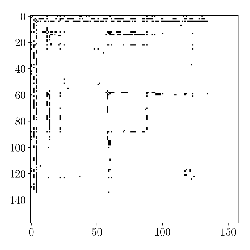
(a) $\mathbf{A}_{t+1}$

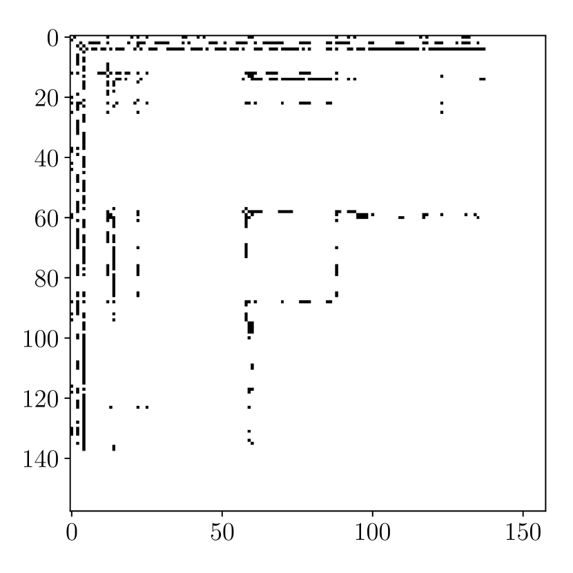
(b) Reconstructed $\mathbf{A}_{t+1}$

Figure 1: Adjacency matrix reconstruction of the mention network #vocesdelareconciliacion. The Rayleigh quotient is used to approximate the eigenvalues of a matrix from a set of orthogonal vectors (eigenvector approximations). The accuracy of these approximations is showed by the comparison between the original matrix and its reconstruction (based on the approximations of the eigenvalues).

4 Case Study: Twitter Conversations

This section presents the results of applying the proposed growth methods to predict evolution of the mention networks between Twitter users. First, the networks are described and the assumptions of the spectral evolution model are verified. Second, the performance of the extended model is analyzed and compared to the performance of the using common methods from the original spectral evolution model.

4.1 Data Description

The dataset consists of $31$ mention networks on Twitter users with a profile location in Colombia. These networks capture conversations around a set of hashtags $H$ related to popular political topics between August $2017$ and August $2018$. Users are represented by the vertex set $V$. The set of edges is denoted by $E$. There exists an edge $(u,v)$ between users $u$ and $v$, if $u$ identifies a message with a political hashtag in $H$ (e.g., #eleccionesseguras) and mentions $v$ (via @username). The mention network $G=(V,E)$ is a simple graph (without self-loops), which means that there is at most one edge between any pair of users. Moreover, every edge $(u,v)\in E$ is associated to a timestamp representing the time at which the edge was created.

The analysis presented in this section is based on the largest connected component of $G$, denoted by $G_{c}=(V_{c},E_{c})$. Networks $G$ and $G_{c}$ are built for each hashtag $h\in H$. Table 1 presents a brief description of each network considered in this study, including its corresponding hashtag, and number of vertices and edges ($|V|$ and $|E|$).

	Set of hashtags $H$	$G$		$G_{c}$
		$|V|$	$|E|$	$|V_{c}|$	$|E_{c}|$
1	abortolegalya	2235	2202	1282	1538
2	alianzasporlaseguridad	176	1074	150	351
3	asiconstruimospaz	2514	14055	2405	6950
4	colombialibredefracking	1606	3483	1476	3127
5	colombialibredeminas	707	2685	655	1421
6	dialogosmetropolitanos	959	18340	932	4134
7	edutransforma	166	1296	161	404
8	eleccionesseguras	3035	17922	2634	7969
9	elquedigauribe	2375	6933	2052	5272
10	frutosdelapaz	1671	6960	1479	3468
11	garantiasparatodos	388	814	340	563
12	generosinideologia	639	914	615	805
13	hidroituangoescololombia	1028	3362	883	2252
14	horajudicialur	2250	23647	2187	6756
15	lafauriecontralor	2154	7082	1999	5309
16	lanochesantrich	1518	6946	1444	3567
17	lapazavanza	2949	8288	2775	6569
18	libertadreligiosa	1584	13443	1395	6856
19	manifestacionpacifica	211	274	112	151
10	plandemocracia2018	3090	20955	2962	7996
21	plenariacm	1504	19866	1460	4782
22	proyectoituango	1214	3086	1186	1891
23	reformapolitica	2714	8385	2608	5928
24	rendiciondecuentas	5103	25479	4401	10308
25	rendiciondecuentas2017	1711	12441	998	2933
26	resocializaciondigna	503	4054	496	1171
27	salariominimo	2494	7041	2079	5016
28	semanaporlapaz	1988	8103	1732	4860
29	serlidersocialnoesdelito	530	861	439	697
30	vocesdelareconciliacion	161	1500	158	405
31	votacionesseguras	2748	13307	2439	5338

Table 1: Description of the mention networks with political hashtags. The analysis is based on the largest connected component of each network, $G_{c}$.

4.2 Verifying the Spectral Evolution Model Assumptions

To apply the original and extended versions of the spectral evolution model, the assumptions on the spectrum and eigenvectors need to be verified. Let $t\in\mathbb{N}$ be a positive number. The set of edges $E$ is sorted by time stamps and then split into $t$ disjoint subsets of equal size ($|E|/t$). Next, consider a total of $t$ time steps, created in a way that each time $i$, $1\leq i\leq t$, contains the edges of the first $i$ subsets of edges. Note that each time step $i$ represents a cumulative graph that is associated to an adjacency matrix $\mathbf{A}_{i}$ and its spectral decomposition $\mathbf{X}_{i}\mathbf{\Lambda}_{i}\mathbf{X}^{T}_{i}$. Note also that $\mathbf{A}_{1},\mathbf{A}_{2},\dots,\mathbf{A}_{t}$ represents the evolution of the network over time and $\mathbf{A}_{t}=\mathbf{A}$ represents the adjacency matrix of the complete network. Overall, this process takes $O(tn^{3})$ time with $n=|V|$: each spectral decomposition takes $O(n^{3})$ and there are $t$ of such decompositions to compute. Figure 2 summarizes the process of defining a sequence of networks for a particular mention network.

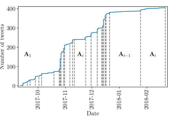
Figure 2: Process of defining a sequence of networks for the mention network #vocesdelareconciliacion based on $t$ time steps. In general, for a network $G=(V,E)$ with adjacency matrix $\mathbf{A}$, the edge set $E$ is split into $t$ disjoint subsets according to their associated time stamps. Time step $i$ contains all the edges of the first $i$ subsets of edges. Note that each time $i$ is associated to an adjacency matrix $\mathbf{A}_{i}$ and $\mathbf{A}_{t}=\mathbf{A}$.

4.2.1 Spectral and Eigenvector Evolution

Figure 3 identifies the largest eigenvalues (by absolute value) for two mention networks: namely, #educationtransforms and #howwebuildpeace. Note that for each of these two networks, the spectra grows irregularly. Consider the adjacency matrix $\mathbf{A}_{1}$ for time $t_{1}$ satisfying $1\leq t_{1}<t$. The eigenvectors ${(\mathbf{X}_{t})}_{j}$ corresponding to the largest eigenvalues are compared to the eigenvectors ${(\mathbf{X}_{1})}_{j}$at time $t$ using the cosine distance as a similarity measure, for each latent dimension $j$.

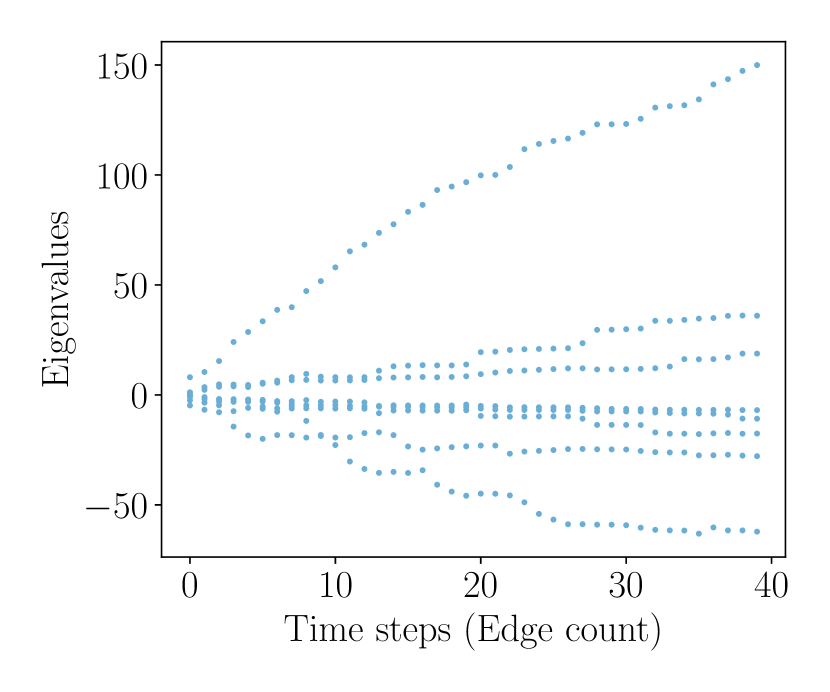
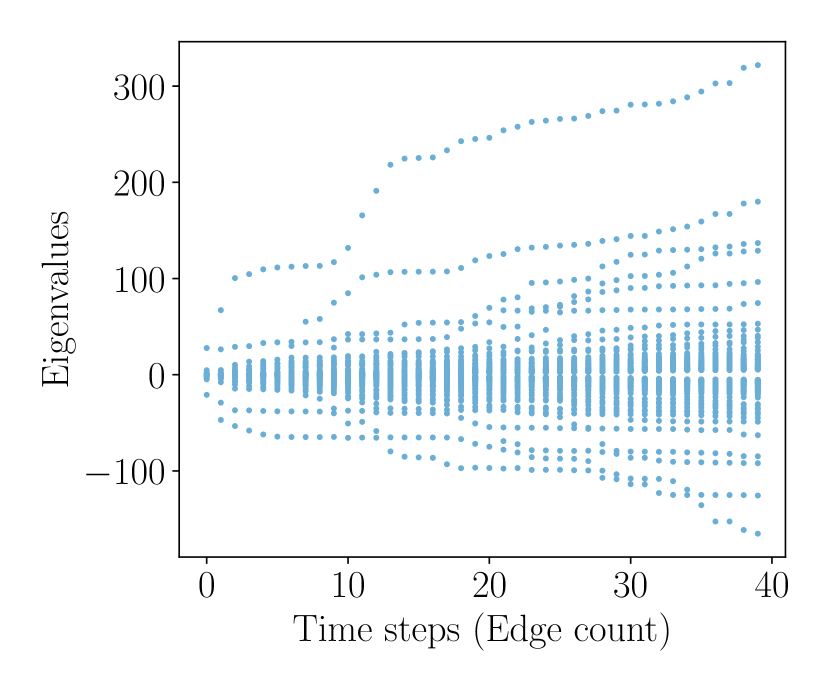
Figure 3: Spectral evolution for two mention networks, #edutransforma (left) and #asiconstruimospaz (right). Plots illustrate the top $8\%$ of the largest eigenvalues by absolute value at each time step.

Figure 4 shows that, during the evolution of the network, certain eigenvectors have a similarity value close to one. They correspond to the eigenvectors associated to the largest eigenvalues. Note also that at points the similarity between some eigenvectors drops to zero, which can be explained by eigenvectors changing their order during the spectral decomposition.

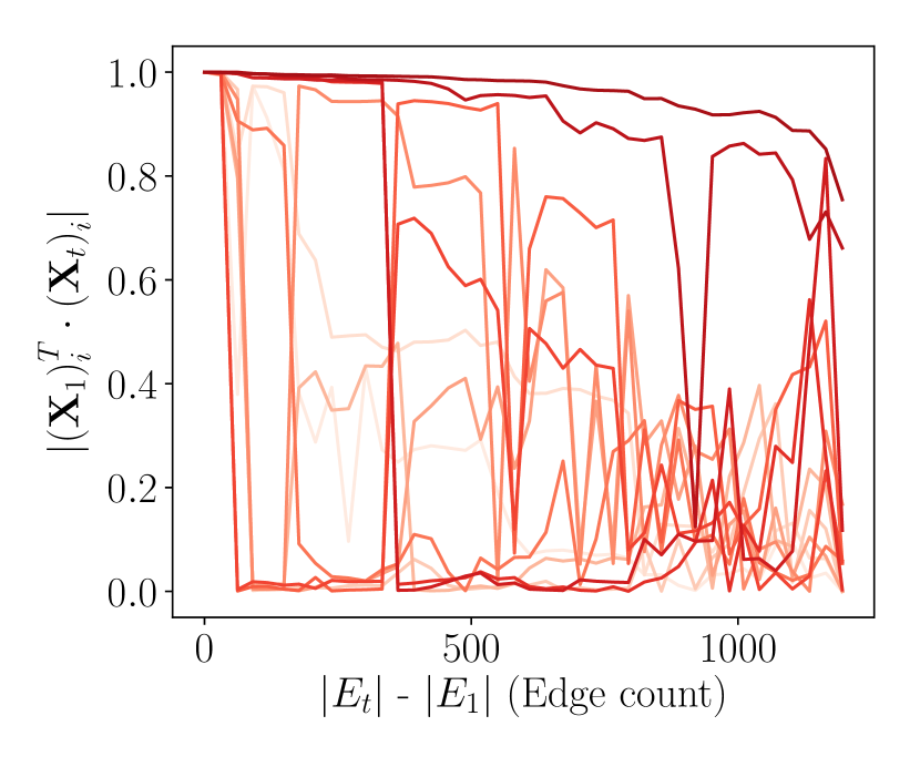
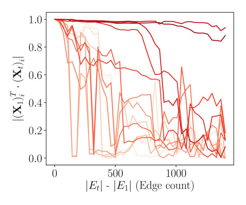
Figure 4: Eigenvector evolution shows a one by one eigenvector comparison between $t_{1}$ and $t$ using the cosine similarity. Each line represents a latent dimension, i.e., a pair of eigenvectors being compared, with brighter colors for eigenvectors corresponding to the largest eigenvalues. Eigenvector evolution for two mention networks, #edutransforma (left) and #vocesdelareconciliacion (right).

4.2.2 Eigenvector Stability

Let $t_{1}$ and $t$ denote the times at which $75\%$ and $100\%$ of all edges in a given network $G$ are present in its adjacency matrices $\mathbf{A}_{1}$ and $\mathbf{A}_{t}$ at times $t_{1}$ and $t$, respectively. Their spectral decomposition is $\mathbf{A}_{1}=\mathbf{X}_{1}\mathbf{\Lambda}_{1}\mathbf{X}^{T}_{1}$ and $\mathbf{A}_{t}=\mathbf{X}_{t}\mathbf{\Lambda}_{t}\mathbf{X}^{T}_{t}$. Similarity values are computed for every pair of eigenvectors $\mathbf{x}_{i}$ and $\mathbf{x}_{j}$ by:

$$\operatorname{sim}_{ij}(t_{1},t)=\left|{(\mathbf{X}_{1})}^{T}_{i}\cdot{(\mathbf{X}_{t})}_{j}\right|.$$

Figure 5 summarizes the resulting values, plotted as a heatmap. White cells represent a value of zero and black cells a value of one. The more the heatmap approximates a diagonal matrix, the fewer eigenvector permutations there are (i.e., the eigenvectors are preserved over time). Note that the value of certain cells in Figure 5 is between zero and one. These cells result either from an exchange in the location of eigenvectors that have eigenvalues very close in magnitude or from comparing eigenvalues ${({\lambda}_{1})}_{i}$ and ${({\lambda}_{t})}_{i}$ that do not correspond to each other.

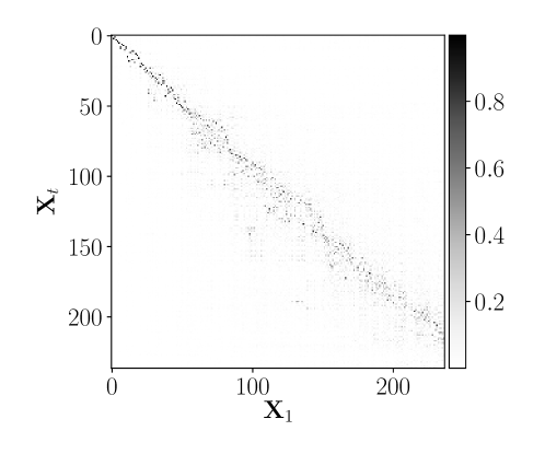
Figure 5: Eigenvector stability for the mention network #plandemocracia2018. Similarity measure for every pair of eigenvectors between $t_{1}$ and $t$. A similarity value of zero is represented by a white square and a similarity of one by a black square. The matrix illustrates the permutations of the eigenvectors. A diagonal matrix represents the case where eigenvectors are preserved over time.

4.2.3 Spectral Diagonality Test

Recall the spectral decomposition $(\mathbf{X}_{1},\mathbf{\Lambda}_{1})$ of $\mathbf{A}_{1}$ from Section 4.2.2, representing the network $G$ at time $t_{1}$. At any time $t_{2}>t_{1}$, the adjacency matrix $\mathbf{A}_{2}$ is expected to have the form $\mathbf{A}_{2}=\mathbf{X}_{1}(\mathbf{\Lambda}_{1}+\mathbf{\Delta})\mathbf{X}^{T}_{1}$, where $\mathbf{\Delta}$ is a diagonal matrix. The diagonal matrix $\mathbf{\Delta}$ can be used to infer if the network’s growth is related to the eigenvalues. Technically, by using least-squares, the matrix $\mathbf{\Delta}$ can be derived as $\mathbf{\Delta}=\mathbf{X}_{1}(\mathbf{A}_{2}-\mathbf{A}_{1})\mathbf{X}^{T}_{1}$. If $\mathbf{\Delta}$ is diagonal, then the growth between $t_{1}$ and $t_{2}$ is spectral. Figure 6 shows the diagonality test for the mention network #plandemocracia2018. It has been found that most of the networks in the dataset show irregular behavior in the spectrum evolution. Note that the matrix $\mathbf{\Delta}$ (spectral diagonality) is almost diagonal for all mention networks.

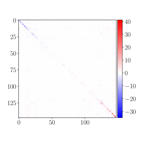
Figure 6: The spectral diagonality test shows to what extent the network evolution is explained by the eigenvalues. If network growth is related to spectrum evolution, then the matrix should be approximately diagonal. Spectral diagonality test for the mention network #plandemocracia2018.

4.3 Prediction Performance

First, the prediction performance of the proposed approach (Section 3) is compared to that of the spectral evolution model (Section 2). In each case, the performance of the prediction is measured by the AUC ROC score. Figure 7 summarizes the performance comparison of the growth methods when exact spectral decomposition and trajectories approximations with the Rayleigh quotient. Note that for most of the networks and growth methods, the performance of the two approaches is highly similar. One conclusion to draw is that it is possible to replicate the prediction of the exact method with the more efficient method based on approximations. A $75\%$-$25\%$ train-test split was used for the analysis depicted in Figure 7. This ratio can be interpreted as $75\%$ of edges of the network (by creation time) are used to predict the remaining $25\%$. The proposed approach is used for the remainder of the analysis in this section.

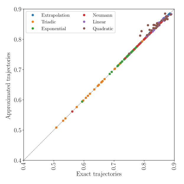
Figure 7: Performance comparison of using exact spectral decomposition and the proposed approach where spectrum trajectories are approximated using the Rayleigh quotient. The comparison is measured by the AUC ROC score. Both methods seem to be consistent, i.e., the performance of the prediction is replicated using the Rayleigh quotient method.

Reducing the number of steps to be predicted while avoiding overfitting, can bring performance improvement of the prediction. Figure 8 shows a comparison of the performance for the $75\%$ and $80\%$ split ratios. Note that reducing the size of test set (and increasing train set) comes with noticeable improvement in the performance of the methods, in general. It has been verified that the growth of the spectrum is irregular for most of the networks. Therefore, it is expected that methods based on extrapolation, and linear and quadratic regression, outperform the ones based on graph kernels.

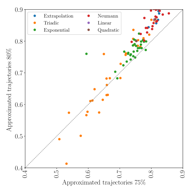
Figure 8: Comparison of the prediction performance based on AUC ROC score for $75\%$ and $80\%$ train-test ratios. Increasing the train set size improves the overall performance of the growth methods.

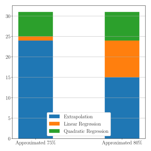
Figure 9: With a $75\%$-$25\%$ train-test ratio for the prediction, the extrapolation method outperforms the regression methods for 24 out of the 31 analyzed networks. When the train set size increases to $80\%$, the regression methods outperform the extrapolation methods for 16 networks.

It is important to include the AUC ROC score to evaluate the methods. For instance, if the initial train-test ratio for both methods is considered, the extrapolation method seems to outperform the other methods in many cases. Its score is the best 24 times in total. But the situation changes when the size of the training set size increases: if the ratio is $80\%$, the regression methods get better score for 16 out of 31 networks (9 and 7 for the linear and quadratic regressions, respectively). As depicted in Figure 9, the distribution of the best method changes alongside the modification of the train-test ratio. Improvement in the regression methods is explained by the addition of new data available for the prediction. Figure 10 shows the improvement of the AUC ROC score in percentage with respect to the $75\%$-$25\%$ ratio.

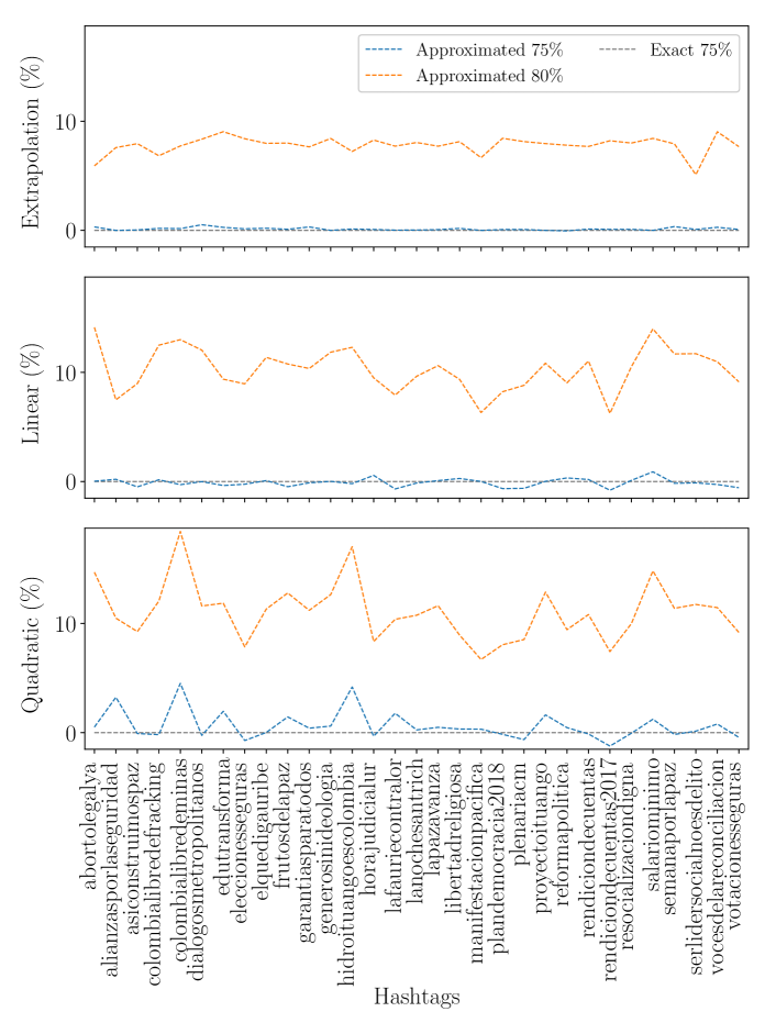
Figure 10: Improvement of the AUC ROC score in percentage computed with the Rayleigh quotient considering different train-test ratios for extrapolation (top), linear (middle) and quadratic (bottom) growth methods w.r.t. the spectral decomposition method. Performance of the regression methods improve more than $10\%$ on average.

Finally, execution times of both approaches are analyzed. Figure 11 (top) shows the cumulative execution time of using the spectral evolution model with exact spectral decomposition ($75\%$) and the extended spectral evolution model with approximated spectra ($75\%$, $80\%$) when used on all 31 mention networks. Note that there is noticeable difference (more than $\numprint{10000}$ seconds) between the execution time of the two approaches. Considering the difference between the methods for each network, the average improvement in favor of the extended evolution model is $71.5\%$. The bottom plot in Figure 11 summarizes the execution time improvement in percentage for each network, ranging from $45\%$ to $80\%$. Note that the spectral extrapolation, linear and quadratic regression outperform the graph kernels. Better prediction in the extrapolation-based approaches seems to be consequence of their ability to capture the irregular evolution of the eigenvalues. Also, linear and quadratic regressions improve their performance when the size of the train test increases.

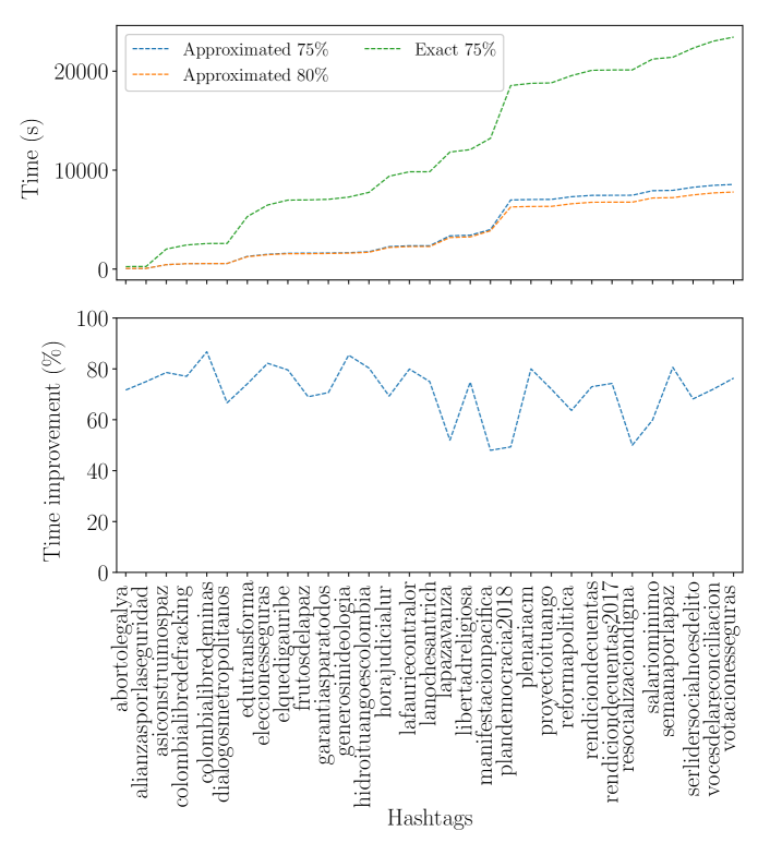
Figure 11: Cumulative execution time of using the spectral evolution model with exact spectral decomposition ($75\%$) and the extended spectral evolution model with approximated spectra ($75\%$, $80\%$) when used on all 31 mention networks (top) and average execution time improvement (bottom).

5 Conclusion and Future Work

This paper extended the spectral evolution model (Kunegis et al., 2013) to estimate link prediction in complex networks. It characterizes the evolution of a network in terms of the evolution of its spectrum, i.e., the eigenvalues of its adjacency matrix. On the one hand, the proposed approach uses the Rayleigh quotient for fast computation of eigenvalue approximations. On the other hand, the estimation of new edges formation is cast as the problem of predicting eigenvalues’ trajectories. In particular, linear and quadratic regression methods showcase the proposed approach. It has been validated that in the growth of some Twitter mention networks, the eigenvectors remain largely constant, while their spectrum grows irregularly. Since computing the spectral decomposition at every time step for each network is a computationally expensive task, the Rayleigh quotient proved to be a feasible tool to efficiently calculating the approximated eigenvalues trajectories. It also avoids the exchange in the location of eigenvectors seen in stability tests. It was further observed that the prediction performance of some methods improve by modifying the train-test ratio in such a way that the size of the train set increases. Especially, the performance of the linear and quadratic regression methods are enhanced because the ratio modifications include more available information for the prediction. Also, the execution time reduction introduced by the Rayleigh quotient is noteworthy. In fact, the analysis using this technique is twice as fast, in comparison to other common techniques, for most of the Twitter mention networks studied here. For experimentation, this was crucial because accessing large networks became an option. Based on the extensive experimental exploration summarized in this manuscript, the authors strongly believe that proposed approach has the potential to become a significant addition to the spectral evolution model approach.

For future research, the use of matrix representations other than the adjacency matrix need to be researched. In general, it is known that eigenvalues and eigenvectors are most meaningful when used to understand a natural operator or a natural quadratic form, such as the Laplacian matrix. In applications, it would be interesting to apply the approach to other networks such as gene co-expression networks, where genes represent vertices and there is a link between two genes $g_{1}$ and $g_{2}$ if there is a positive relation in their expression, i.e., $g_{1}$ and $g_{2}$ use to express at the same time (Ruan et al., 2010; Stuart et al., 2003). In this case, new relations in the gene co-expression can be predicted through the extended spectral evolution model. Finally, considering different growth methods in the analysis in order to capture more information from the spectrum of the networks remains an important research direction.

References

- Chatelin (2012) Chatelin, F. (2012). Eigenvalues of Matrices: Revised Edition. Philadelphia, PA: Society for Industrial and Applied Mathematics.
- DiMaggio et al. (1996) DiMaggio, P., Evans, J., & Bryson, B. (1996). Have American’s Social Attitudes Become More Polarized? American Journal of Sociology, 102(3), 690–755.
- Godsil & Royle (2001) Godsil, C., & Royle, G. (2001). Algebraic Graph Theory, vol. 207 of Graduate Texts in Mathematics. Springer.
- Gong et al. (2018) Gong, Q., Chen, Y., He, X., Zhuang, Z., Wang, T., Huang, H., Wang, X., & Fu, X. (2018). DeepScan: Exploiting Deep Learning for Malicious Account Detection in Location-Based Social Networks. IEEE Communications Magazine, 56(11), 21–27.
- Ince (2013) Ince, M. (2013). Filling the FARC-Shaped Void: Potential Insecurity in Post-Conflict Colombia. The RUSI Journal, 158(5), 26–34.
- Jalili et al. (2017) Jalili, M., Orouskhani, Y., Asgari, M., Alipourfard, N., & Perc, M. (2017). Link prediction in multiplex online social networks. Royal Society Open Science, 4(2), 160863.
- Kunegis et al. (2013) Kunegis, J., Fay, D., & Bauckhage, C. (2013). Spectral evolution in dynamic networks. Knowledge and Information Systems, 37(1), 1–36.
- Kurucz et al. (2009) Kurucz, M., Benczúr, A. A., Csalogány, K., & Lukács, L. (2009). Spectral clustering in social networks. In Advances in Web Mining and Web Usage Analysis, (pp. 1–20). Berlin, Heidelberg: Springer Berlin Heidelberg.
- Martinčić-Ipšić et al. (2017) Martinčić-Ipšić, S., Močibob, E., & Perc, M. (2017). Link prediction on Twitter. PLOS ONE, 12(7), e0181079.
- Romero et al. (2020) Romero, M., Rocha, C., & Finke, J. (2020). Spectral evolution of Twitter mention networks. In H. Cherifi, S. Gaito, J. F. Mendes, E. Moro, & L. M. Rocha (Eds.) Complex Networks and Their Applications VIII, vol. 881, (pp. 532–542). Cham: Springer International Publishing.
- Ruan et al. (2010) Ruan, J., Dean, A. K., & Zhang, W. (2010). A general co-expression network-based approach to gene expression analysis: Comparison and applications. BMC Systems Biology, 4(1), 8.
- Saab & Taylor (2009) Saab, B. Y., & Taylor, A. W. (2009). Criminality and Armed Groups: A Comparative Study of FARC and Paramilitary Groups in Colombia. Studies in Conflict & Terrorism, 32(6), 455–475.
- Stuart et al. (2003) Stuart, J. M., Segal, E., Koller, D., & Kim, S. K. (2003). A Gene-Coexpression Network for Global Discovery of Conserved Genetic Modules. Science, 302(5643), 249–255.