Two-photon exchange from intermediate state resonances
in elastic electron-proton scattering

Abstract

We use a recently developed dispersive approach to compute the two-photon exchange (TPE) correction to elastic electron-proton scattering, including contributions from hadronic $J^{P}=1/2^{\pm}$ and $3/2^{\pm}$ resonant intermediate states below 1.8 GeV. For the transition amplitudes from the proton ground state to the resonant excited states we employ new exclusive meson electroproduction data from CLAS at $Q^{2}\lesssim 5$ GeV², and we explore the effects of both fixed and dynamic widths for the resonances. Among the resonant states, the $N(1520)~{}\!3/2^{-}$ becomes dominant for $Q^{2}\gtrsim 2$ GeV², with a sign opposite to the comparably sized $\Delta(1232)~{}\!3/2^{+}$ contribution, leading to an overall increase in the size of the TPE correction to the cross section relative to the nucleon only contribution at higher $Q^{2}$ values. The results are in good overall agreement with recent $e^{+}p$ to $e^{-}p$ cross section ratio and polarization transfer measurements, and provide compelling evidence for a resolution of the electric to magnetic form factor ratio discrepancy.

I Introduction

Elastic electron–nucleon scattering has been one of the most indispensable tools to probe the internal structure of nucleons through the determination of their electromagnetic form factors. For many decades the proton’s electric ($G_{E}(Q^{2})$) and magnetic ($G_{M}(Q^{2})$) elastic form factors have been measured in unpolarized scattering experiments using the Rosenbluth longitudinal-transverse (LT) separation technique Walker et al. (1994); Andivahis et al. (1994); Qattan et al. (2005). These experiments found that the ratio $\mu_{p}\,G_{E}/G_{M}$, where $\mu_{p}$ is the proton’s magnetic moment, are consistent with 1 over a large range of the four-momentum transfer squared, $Q^{2}$, up to 8.83 GeV². More recently, measurements of the electric to magnetic form factor ratio with significantly reduced uncertainties were performed at Jefferson Lab using the polarization transfer (PT) technique Jones et al. (2000); Gayou et al. (2002); Punjabi et al. (2005); Puckett et al. (2010, 2012). These experiments found a linear fall-off of the ratio $\mu_{p}\,G_{E}/G_{M}$ from 1 with increasing $Q^{2}$ in the range up to 8.5 GeV².

Analysis of the LT separation electron scattering data has traditionally been performed within the one-photon exchange (OPE) approximation. The electric to magnetic form factor ratio discrepancy motivated studies of hadron structure-dependent two-photon exchange (TPE) radiative corrections, and it was generally believed that the problem would be resolved with the inclusion of these effects Blunden et al. (2003); Guichon and Vanderhaeghen (2003). Subsequent years have seen a growing sophistication in the theoretical efforts that have been made to better understand the TPE phenomena using various approaches. These have included using hadronic models to compute the real part of the TPE amplitude through loop integrals with (on-shell) transition form factors Blunden et al. (2005); Kondratyuk et al. (2005); Kondratyuk and Blunden (2007); Zhou and Yang (2015), dispersive approaches Borisyuk and Kobushkin (2008, 2012, 2015); Tomalak and Vanderhaeghen (2015); Blunden and Melnitchouk (2017), use of generalized parton distributions to model the high-energy behavior of the intermediate state hadrons at the quark level Chen et al. (2004); Afanasev et al. (2005), and QCD factorization approaches Borisyuk and Kobushkin (2009); Kivel and Vanderhaeghen (2009).

The use of hadronic degrees of freedom can be considered as a reasonable approximation for low to moderate values of $Q^{2}\lesssim 5$ GeV², where hadrons are expected to retain their identity. However, for excited intermediate states of higher spin, such as the $\Delta$ isobar, in the forward angle limit Blunden and Melnitchouk (2017) the direct loop-integral approach gives rise to unphysical divergences in the TPE amplitude at forward angles. This problem of unphysical behavior can be resolved using the dispersive method described in Refs. Gorchtein (2007); Borisyuk and Kobushkin (2008, 2014, 2015); Tomalak and Vanderhaeghen (2015); Tomalak et al. (2017); Blunden and Melnitchouk (2017), where the on-shell form factors are used explicitly to calculate the imaginary part of the TPE amplitude from unitarity, with the real part then obtained from a dispersion integral.

In this work we follow the dispersive approach for resonant intermediate states developed in Ref. Blunden and Melnitchouk (2017). Unlike previous calculations which made use of the narrow resonance approximation, here we allow a Breit-Wigner shape with a nonzero width for each individual resonance, with either a fixed width or a dynamical width that depends on the final state hadron mass. Furthermore, in addition to the $\Delta(1232)~{}\!3/2^{+}$ resonance, we also compute the TPE contribution from all the established $J^{P}=1/2^{\pm}$ and $3/2^{\pm}$ states below 1.8 GeV, including the $N(1440)~{}\!1/2^{+}$ Roper resonance, $N(1520)~{}\!3/2^{-}$, $N(1535)~{}\!1/2^{-}$, $\Delta(1620)~{}\!1/2^{-}$, $N(1650)~{}\!1/2^{-}$, $\Delta(1700)~{}\!3/2^{-}$, $N(1710)~{}\!1/2^{+}$, and $N(1720)~{}\!3/2^{+}$ resonances. With the exception of the $\Delta(1232)~{}\!3/2^{+}$, for which we use the fit by Aznauryan and Burkert Blunden and Melnitchouk (2017); Aznauryan and Burkert (2012), for the resonance electrocouplings at the hadronic vertices we use the most recent helicity amplitudes extracted from the analysis of CLAS meson electroproduction data Hiller Blin et al. (2019); Mokeev et al. (2012, 2009).

We begin in Sec. II by describing the kinematics of the elastic $e^{-}p$ scattering process, both in the one- and two-photon exchange approximations. Details of the TPE calculations for the resonance states are presented in Sec. III, where we summarize the formal relations for the resonance transition current operators in terms of the form factors $G_{i}$ (Sec. III.1), and relate the form factors to the helicity amplitudes (Sec. III.2). The dispersive method and its practical implementation are discussed in Sec. III.3, where we express the TPE amplitudes and cross sections in terms of the generalized TPE form factors. Numerical results for the TPE corrections are presented in Sec. IV, where the effects of finite widths (Sec. IV.2) and the role of spin, isospin and parity of the intermediate states (Sec. IV.3) are discussed. Comparisons with experimental observables sensitive to TPE contributions are made in Sec. V. Finally, conclusions and future outlook of our work are presented in Sec. VI.

II Electron-Proton Elastic Scattering

The kinematics of the elastic electron–proton scattering process are shown in Fig. 1 for the one-photon exchange (or Born) approximation and for the TPE contribution. Here an electron with four-momentum $k=(E,\bm{k})$ is scattered from a proton initially at rest, $p=(M,0)$ in the target rest frame, to an electron in the final state with four-momentum $k^{\prime}=(E^{\prime},\bm{k^{\prime}})$. The transferred four-momentum from the electron to the proton is $q=k-k^{\prime}$, and the proton recoils with four-momentum $p^{\prime}=p+q$. For the TPE diagram, two virtual photons of four-momenta $q_{1}$ and $q_{2}$ are exchanged, with $q=q_{1}+q_{2}$.

II.1 One-photon exchange

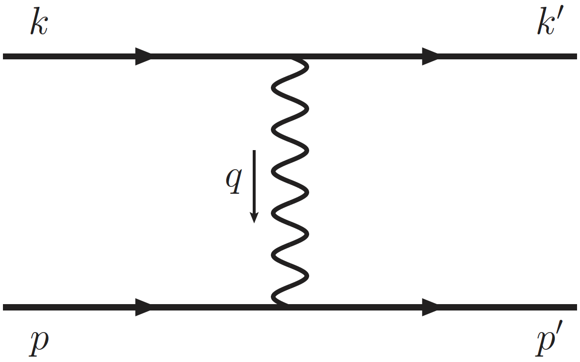
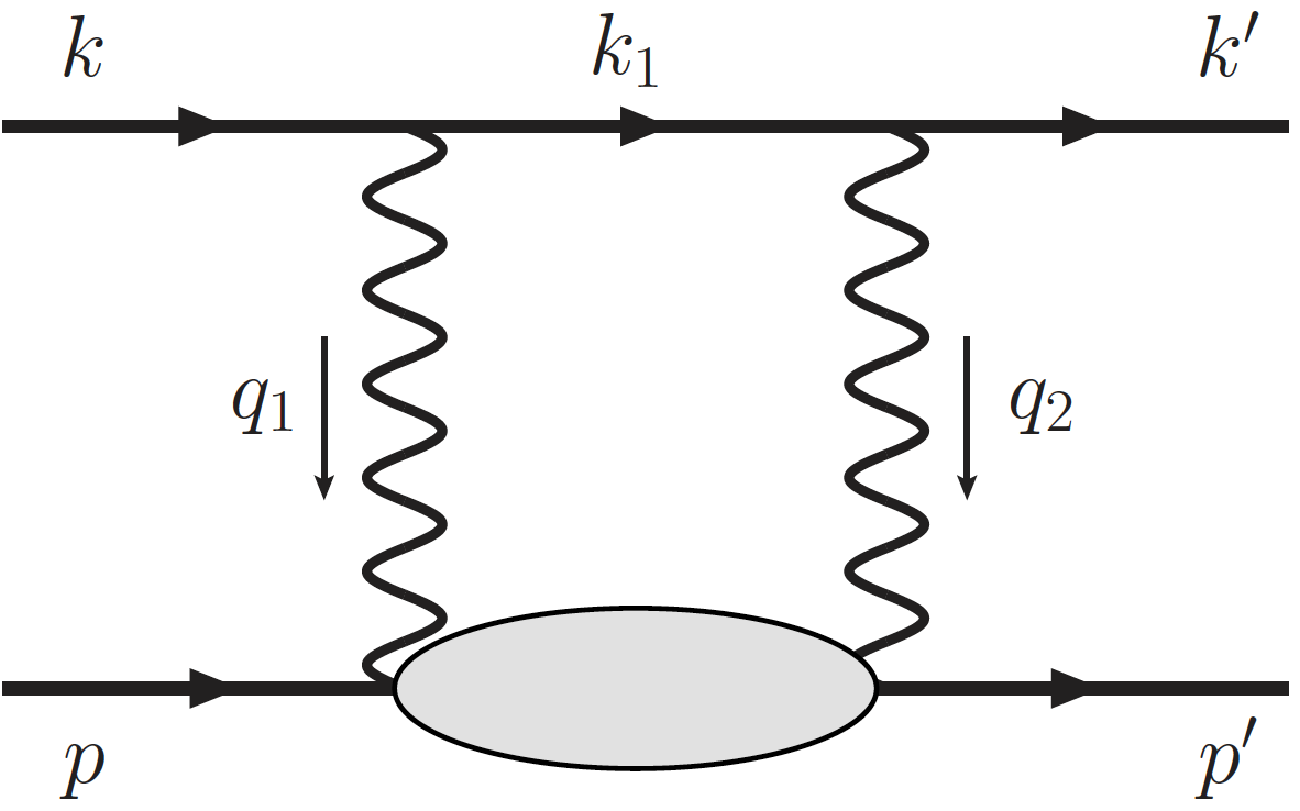
Figure 1: Elastic scattering of an electron (four-momentum $k$) from a proton ($p$) to a final state electron ($k^{\prime}$) and recoil proton ($p^{\prime}$), with $q=k-k^{\prime}=p^{\prime}-p$ the four-momentum transfer, in the Born approximation (left panel) and for the two-photon exchange process (right panel). Only the $s$-channel box diagram is shown for the TPE correction, in which the two photons carry momenta $q_{1}$ and $q_{2}$, and the crossed box contribution can be obtained using the $s\to u$ crossing symmetry.

For the one-photon exchange approximation, the amplitude ${\cal M}_{\gamma}$ for scattering an electron from a proton can be written as Arrington et al. (2011)

$${\cal M}_{\gamma}=e^{2}\,j_{\mu}\,\dfrac{1}{Q^{2}}\,J^{\mu},$$ (1)

where $e$ is the charge of the proton, and the total four-momentum transfer squared $Q^{2}$ can be written in terms of the electron energy $E$ and scattering angle $\theta$ as $Q^{2}\equiv-q^{2}=4EE^{\prime}\sin^{2}(\theta/2)$. The electron transition current is given by $j_{\mu}=\bar{u}_{e}(k^{\prime})\,\gamma_{\mu}\,u_{e}(k)$, while the proton transition current is $J^{\mu}=\bar{u}_{N}(p^{\prime})\,\Gamma^{\mu}(q)\,u_{N}(p)$, where the hadronic current operator $\Gamma^{\mu}$ is parameterized through form factors that take into account the proton’s internal structure. For on-shell particles, current conservation at the hadron vertex allows for two independent Lorentz vectors, so the hadronic current operator is typically parameterized in terms of the Dirac $F_{1}$ and Pauli $F_{2}$ form factors,

$$\Gamma^{\mu}(q)=F_{1}(Q^{2})\gamma^{\mu}+F_{2}(Q^{2})\dfrac{\textit{i}\sigma^{\mu\nu}q_{\nu}}{2M},$$ (2)

where $M$ is the proton mass. It is often convenient to use the Sachs electric and magnetic form factors $G_{E}$ and $G_{M}$, which are defined as linear combinations of the Dirac and Pauli form factors,

$$G_{E}(Q^{2})=F_{1}(Q^{2})-\tau F_{2}(Q^{2}),\ \ \ \ \ \ \ G_{M}(Q^{2})=F_{1}(Q^{2})+F_{2}(Q^{2}),$$ (3)

where $\tau=Q^{2}/4M^{2}$. The differential cross section for single photon exchange is proportional to the square of the scattering amplitude ${\cal M}_{\gamma}$, and can be expressed in terms of the electric and magnetic form factors as

$$\bigg{(}\dfrac{d\sigma}{d\Omega}\bigg{)}_{0} = \left(\dfrac{\alpha E^{\prime}}{4MQ^{2}E}\right)^{2}\left|{\cal M}_{\gamma}\right|^{2}\,=\,\dfrac{\sigma_{\rm Mott}}{\varepsilon(1+\tau)}\,\sigma_{R}^{\rm{Born}},$$ (4)

where $\alpha=e^{2}/4\pi$ is the electromagnetic fine structure constant, and

$$\varepsilon=\left[1+2\left(1+\tau\right)\tan^{2}\left(\theta/2\right)\right]^{-1}$$ (5)

is the virtual photon polarization. In Eq. (4) the reduced cross section $\sigma_{R}^{\rm{Born}}$ is given by

$$\sigma_{R}^{\rm{Born}}=\varepsilon G_{E}^{2}(Q^{2})+\tau G_{M}^{2}(Q^{2}),$$ (6)

and the Mott cross section,

$$\sigma_{\rm Mott}=\dfrac{4\alpha^{2}E^{\prime 3}\cos^{2}(\theta/2)}{EQ^{4}},$$ (7)

gives the cross section for scattering an electron from a point target.

II.2 Two-photon exchange

The two-photon exchange amplitude, ${\cal M}_{\gamma\gamma}$, is the sum of contributions from the box diagram of Fig. 1 and the corresponding crossed-box diagram (not shown),

$${\cal M}_{\gamma\gamma}={\cal M}_{\gamma\gamma}^{\rm{box}}+{\cal M}_{\gamma\gamma}^{\rm{xbox}}.$$ (8)

In general, the box diagram amplitude ${\cal M}_{\gamma\gamma}^{\rm{box}}$ can be written as an integral over loop momenta $q_{1}$ or $q_{2}$ of the exchanged photons Arrington et al. (2011),

$${\cal M}_{\gamma\gamma}^{\rm{box}}=-ie^{4}\int\!\dfrac{d^{4}q_{1}}{(2\pi)^{4}}\dfrac{L_{\mu\nu}H^{\mu\nu}}{(q_{1}^{2}-\lambda^{2})(q_{2}^{2}-\lambda^{2})},$$ (9)

where an infinitesimal photon mass $\lambda$ is introduced to regulate infrared divergences. The leptonic tensor $L_{\mu\nu}$ in Eq. (9) is given by

$$L_{\mu\nu}=\bar{u}_{e}(k^{\prime})\gamma_{\mu}S_{F}(k_{1},m_{e})\gamma_{\nu}u_{e}(k),$$ (10)

where $k_{1}=k-q_{1}$ is the intermediate lepton four-momentum, $m_{e}$ is the electron mass (which can in practice be taken to zero at the kinematics considered here), and $S_{F}$ is the electron propagator defined by

$$S_{F}(k_{1},m_{e})=\dfrac{(\not{k}_{1}+m_{e})}{k_{1}^{2}-m_{e}^{2}+i0^{+}}.$$ (11)

The hadronic tensor $H^{\mu\nu}$ can be expressed as

$$H^{\mu\nu}=\bar{u}_{N}(p^{\prime})\,\Gamma_{R\to\gamma N}^{\mu\alpha}(p_{R},-q_{2})\,S_{\alpha\beta}(p_{R},W)\,\Gamma_{\gamma N\to R}^{\beta\nu}(p_{R},q_{1})\,u_{N}(p),$$ (12)

in terms of the transition operators $\Gamma^{\beta\nu}_{\gamma N\to R}$ and $\Gamma^{\mu\alpha}_{R\to\gamma N}$ between the initial nucleon and intermediate resonance $R$ states, where $p_{R}=p+q_{1}=p^{\prime}-q_{2}$ is the four-momentum of the resonance and $W$ its (in principle running) mass.

For spin $1/2$ baryon intermediate states the propagator $S_{\alpha\beta}(p_{R},W)$ reduces to the usual spin-$1/2$ propagator,

$$S_{\alpha\beta}(p_{R},W)=\delta_{\alpha\beta}\dfrac{(\not{p}_{R}+W)}{p_{R}^{2}-W^{2}+i0^{+}}=\delta_{\alpha\beta}\,S_{F}(p_{R},W),$$ (13)

for a particle with mass $W$. The hadronic tensor for spin-1/2 baryons can then be written

$$H^{\mu\nu}=\bar{u}_{N}(p^{\prime})\,\Gamma_{R\to\gamma N}^{\mu}(p_{R},-q_{2})\,S_{F}(p_{R},W)\,\Gamma_{\gamma N\to R}^{\nu}(p_{R},q_{1})\,u_{N}(p),$$ (14)

where the operator $\Gamma_{\gamma N\to R}$ describes the transition to a baryon resonance with spin 1/2.

For the hadronic propagator of spin-3/2 states we use the form

$$S_{\alpha\beta}(p_{R},W)=-{\cal P}_{\alpha\beta}^{3/2}(p_{R})\,\dfrac{(\not{p}_{R}+W)}{p_{R}^{2}-W^{2}+i0^{+}},$$ (15)

where the spin-3/2 projection operator ${\cal P}_{\alpha\beta}^{3/2}$ is defined by

$${\cal P}_{\alpha\beta}^{3/2}(p_{R})=g_{\alpha\beta}-\dfrac{1}{3}\gamma_{\alpha}\gamma_{\beta}-\dfrac{1}{3p_{R}^{2}}\left(\not{p}_{R}\gamma_{\alpha}(p_{R})_{\beta}+(p_{R})_{\alpha}\gamma_{\beta}\not{p}_{R}\right),$$ (16)

The resonance transition currents $\Gamma_{\gamma N\to R}^{\beta\nu}(p_{R},q_{1})$ and $\Gamma_{R\to\gamma N}^{\mu\alpha}(p_{R},-q_{2})$ at the two hadron vertices can be parameterized using the form factors $G_{1},G_{2}$ and $G_{3}$. Details of the transition current are discussed in Sec. III.

The TPE crossed-box amplitude ${\cal M}_{\gamma\gamma}^{\rm{xbox}}$ can be calculated by replacing the lepton tensor $L_{\mu\nu}$ in Eq. 9 by the tensor

$$L_{\mu\nu}^{\rm{xbox}}=\bar{u}_{e}(k^{\prime})\,\gamma_{\nu}\,S_{F}(k_{2},m_{e})\,\gamma_{\mu}u_{e}(k),$$ (17)

where the intermediate lepton momentum is $k_{2}=k-q_{2}$. The crossed-box amplitude can also be obtained from the crossing symmetry relation Blunden and Melnitchouk (2017)

$${\cal M}_{\gamma\gamma}^{\rm{xbox}}(u,t)=-M_{\gamma\gamma}^{\rm{box}}(s,t)\Big{|}_{s\to u},$$ (18)

where the Mandelstam variables $s$, $t$, and $u$ are defined by

$$\begin{aligned} s&=(k+p)^{2}=(k^{\prime}+p^{\prime})^{2},\\ t&=(k-k^{\prime})^{2}=q^{2},\\ u&=(p-k^{\prime})^{2}=(p^{\prime}-k)^{2}.\end{aligned}$$ (19)

Note, however, that, unlike the box amplitude, which is complex, the crossed-box amplitude is purely real. In the dispersive approach it is therefore not necessary to consider the crossed-box term explicitly. Including the one- and two-photon exchange contributions, the total squared amplitude can be written

$$\left|{\cal M}_{\gamma}+{\cal M}_{\gamma\gamma}\right|^{2} \approx \left|{\cal M}_{\gamma}\right|^{2}+2\operatorname{Re}({\cal M}_{\gamma}^{\dagger}{\cal M}_{\gamma\gamma})$$ (20)

$$\equiv \left|{\cal M}_{\gamma}\right|^{2}(1+\delta_{\gamma\gamma}),$$

where terms of order $\alpha^{4}$ have been neglected, and we have defined the relative two-photon exchange correction to the cross section as

$$\delta_{\gamma\gamma}=\dfrac{2\operatorname{Re}({\cal M}_{\gamma}^{\dagger}{\cal M}_{\gamma\gamma})}{|{\cal M}_{\gamma}|^{2}}.$$ (21)

For the nucleon intermediate state the TPE cross section correction is infrared (IR) divergent in the soft photon limit, but this divergence is exactly cancelled by a corresponding divergence in the real photon emission from the electron and proton Maximon and Tjon (2000); Arrington et al. (2011). It is useful, however, to define a finite TPE correction which has the IR divergent contribution subtracted. This correction will not be unique, as it depends on the prescription used for the regularization Mo and Tsai (1969); Maximon and Tjon (2000); Arrington et al. (2011); Blunden and Melnitchouk (2017). For most of the theoretical results presented in this analysis we use the prescription of Maximon and Tjon Maximon and Tjon (2000),

$$\delta=\delta_{\gamma\gamma}(\rm{unsubtracted})-\delta_{\rm{IR}}(\rm{MTj}).$$ (22)

However, most experimental analyses use the prescription of Mo and Tsai Mo and Tsai (1969), and for comparison with experimental data we incorporate the additional correction $\delta_{\rm{IR}}(\rm{MTj})-\delta_{\rm{IR}}(\rm{MTs})$. A discussion of the differences between $\delta_{\rm{IR}}(\rm{MTj})$ of Maximon-Tjon Maximon and Tjon (2000) and $\delta_{\rm{IR}}(\rm{MTs})$ of Mo-Tsai Mo and Tsai (1969) can be found in Ref. Arrington et al. (2011).

III Two-photon exchange from resonant intermediate states

In this work we present the general decomposition of the hadronic transition current operators and parameterize these in terms of the transition form factors $G_{i}$ ($i=1,2,3$) as defined in Ref. Jones and Scadron (1973); Devenish et al. (1976); Aznauryan and Burkert (2012). For our numerical calculation of the imaginary part of the TPE amplitude we use input on the electromagnetic helicity amplitudes $A_{1/2}$, $A_{3/2}$ and $S_{1/2}$ from the analysis of exclusive meson electroproduction data from CLAS at Jefferson Lab Hiller Blin et al. (2019). We provide the explicit relations between the form factors and the helicity amplitudes for the proton to resonance transitions for the spin-parity $1/2^{\pm}$ and $3/2^{\pm}$ excited states in Sec. III.2. Following this, in Sec. III.3 we describe the details of the dispersive method utilized in our study, including the effects of finite resonance widths.

III.1 Resonance transition current operators

We begin this section by parameterizing the transition current operator $\Gamma_{\gamma N\to R}$ describing the absorption of a virtual photon with momentum $q_{1}$ on a nucleon $N$ with momentum $p$, producing a resonant state $R$ with momentum $p_{R}=p+q_{1}$. Following Refs. Devenish et al. (1976); Aznauryan and Burkert (2012), we decompose $\Gamma_{\gamma N\to R}$ into several terms with coefficients defining the form factors $G_{1}$, $G_{2}$ and $G_{3}$. Specifically, for spin-$3/2$ resonant states the current operator has the decomposition

$$\Gamma_{\gamma N\to R}^{\beta\nu}(p_{R},q_{1})=G_{1}(Q_{1}^{2})\,\Theta_{1}^{\beta\nu}(p_{R},q_{1})+G_{2}(Q_{1}^{2})\,\Theta_{2}^{\beta\nu}(p_{R},q_{1})+G_{3}(Q_{1}^{2})\,\Theta_{3}^{\beta\nu}(p_{R},q_{1}),$$ (23)

where the $\Theta_{i}^{\beta\nu}$ operators are defined as

$$\Theta_{1}^{\beta\nu} = \left(\begin{array}[]{cc}\gamma_{5}\\ {\rm I}\end{array}\right)(\not{q}_{1}g^{\beta\nu}-q_{1}^{\beta}\gamma^{\nu}),$$ (24c)

$$\Theta_{2}^{\beta\nu} = \left(\begin{array}[]{cc}\gamma_{5}\\ {\rm I}\end{array}\right)(q_{1}^{\beta}p_{R}^{\nu}-q_{1}\cdot p_{R}\,g^{\beta\nu}),$$ (24f)

$$\Theta_{3}^{\beta\nu} = \left(\begin{array}[]{cc}\gamma_{5}\\ {\rm I}\end{array}\right)(q_{1}^{\beta}q_{1}^{\nu}-q_{1}^{2}g^{\beta\nu}),$$ (24i)

and the upper and lower rows refer to positive and negative parity states, respectively. For spin-$1/2$ resonances, we define the current operator $\Gamma_{\gamma N\to R}^{\nu}$ as

$$\Gamma_{\gamma N\to R}^{\nu}(p_{R},q_{1})=G_{1}(Q_{1}^{2})\left(\begin{array}[]{cc}\rm I\\ {\gamma_{5}}\end{array}\right)\left(\not{q}_{1}q_{1}^{\nu}-q_{1}^{2}\gamma^{\nu}\right)+G_{2}(Q_{1}^{2})\left(\begin{array}[]{cc}\rm I\\ {\gamma_{5}}\end{array}\right)\left(\not{q}_{1}P^{\nu}-P\cdot q_{1}\,\gamma^{\nu}\right),$$ (25)

where $P=(p+p_{R})/2=p_{R}-q_{1}/2$, and again the upper and lower rows refer to positive and negative parity states, respectively. For the inverse transition $R\to\gamma N$ in Fig. 1, the current operator $\Gamma_{R\to\gamma N}^{\mu\alpha}(p_{R},q_{1})$ for the spin-3/2 states can be obtained using the Hermitian property of the transition matrix element,

$$\Gamma_{R\to\gamma N}^{\mu\alpha}(p_{R},q_{1})=\gamma_{0}\,\big{[}\Gamma_{\gamma N\to R}^{\alpha\mu}(p_{R},q_{1})\big{]}^{\dagger}\,\gamma_{0},$$ (26)

where $q_{1}$ is now the momentum of the outgoing photon. A similar relation also holding for the spin-1/2 operator $\Gamma_{R\to\gamma N}^{\nu}(p_{R},q_{1})$.

III.2 Form factors from electrocouplings

Since the electroproduction of resonance states $R$ is often parameterized in terms of resonance electrocouplings $A_{h}$ Hiller Blin et al. (2019), we define here the transition form factors $G_{i}$ in terms of the amplitudes for specific helicity configurations.

III.2.1 Resonance electrocouplings

The resonance electrocouplings at the hadronic vertices are defined in terms of the matrix elements of the hadron electromagnetic current operator as Aznauryan and Burkert (2012)

$$A_{1/2} = \sqrt{\dfrac{2\pi\alpha}{K}}\dfrac{1}{e}\,\Big{\langle}R,S_{z}^{R}=\tfrac{1}{2}\,\Big{|}\,\epsilon_{\mu}^{+}J^{\mu}_{\rm{em}}\,\Big{|}\,N,S_{z}=-\tfrac{1}{2}\Big{\rangle},$$ (27a)

$$A_{3/2} = \sqrt{\dfrac{2\pi\alpha}{K}}\dfrac{1}{e}\,\Big{\langle}R,S_{z}^{R}=\tfrac{3}{2}\,\Big{|}\,\epsilon_{\mu}^{+}J^{\mu}_{\rm{em}}\,\Big{|}\,N,S_{z}=\tfrac{1}{2}\Big{\rangle},$$ (27b)

$$S_{1/2} = \sqrt{\dfrac{2\pi\alpha}{K}}\dfrac{1}{e}\,\Big{\langle}R,S_{z}^{R}=\tfrac{1}{2}\,\Big{|}\,\dfrac{|\bm{q}_{1}|}{Q_{1}}\epsilon_{\mu}^{0}J^{\mu}_{\rm{em}}\Big{|}\,N,S_{z}=\tfrac{1}{2}\Big{\rangle},$$ (27c)

where $\alpha=e^{2}/4\pi$ is the fine structure constant, and $K$ is the equivalent photon energy at the real photon point, $K=(W^{2}-M^{2})/2W$. The spin projections of the nucleon and resonances $R$ on the $z$-axis are labeled by $S_{z}$ and $S_{z}^{R}$, and $\epsilon_{\mu}^{+,0}$ is the photon polarization vector for transversely or longitudinally polarized photons,

$$\epsilon_{\mu}^{+} = (0;-\bm{\epsilon}^{+}),\ \ \ \ \ \bm{\epsilon}^{+}=-\dfrac{1}{\sqrt{2}}(1,i,0),$$ (28a)

$$\epsilon_{\mu}^{0} = \dfrac{1}{Q_{1}}(|\bm{q}_{1}|;0,0,-q_{1}^{0}).$$ (28b)

The virtual photon three-momentum $\bm{q}_{1}$ is taken to be along the $z$-axis in the rest frame of the resonance $R$, and its magnitude is given in terms of the final state hadron mass $W$ and the photon virtuality $Q_{1}^{2}=|\bm{q}_{1}|^{2}-(q_{1}^{0})^{2}$,

$$|\bm{q}_{1}| = \sqrt{Q_{1}^{2}+\left(\dfrac{W^{2}-M^{2}-Q_{1}^{2}}{2W}\right)^{2}}.$$ (29)

The parameterizations of the resonance electrocouplings obtained from the analysis of CLAS meson electroproduction data at Jefferson Lab Hiller Blin et al. (2019) are at the sharp resonance point. To generate the electrocouplings as a function of the running invariant mass $W$ of the intermediate state, we use the $W$-dependent electrocoupling $A_{h}(W,Q_{1}^{2})$ defined as

$$A_{h}(W,Q_{1}^{2})=\dfrac{W}{W_{R}}\dfrac{|\bm{q}_{1,R}|}{|\bm{q}_{1}|}A_{h}^{R}(Q_{1}^{2}),$$ (30)

which is consistent with the prescription in the JM model of Ref. Ripani et al. (2000); Hiller Blin et al. (2019). In Eq. (30), $A_{h}^{R}$ represents the electrocouplings $A_{1/2}$, $A_{3/2}$ or $S_{1/2}$ at the resonance point, $W_{R}$ is the invariant mass $W$ at the resonance point, and $\bm{q}_{1,R}$ is defined as

$$|\bm{q}_{1,R}| = \sqrt{Q_{1}^{2}+\left(\dfrac{W_{R}^{2}-M^{2}-Q_{1}^{2}}{2W_{R}}\right)^{2}}.$$ (31)

III.2.2 Relations between form factors and electrocouplings

Following Devenish et al. Devenish et al. (1976), the hadronic transition current operator $\Gamma_{\gamma N\to R}^{\beta\nu}$ for spin-3/2 resonances can also be parameterized in terms of helicity form factors $h_{1}$, $h_{2}$ and $h_{3}$, which are given in terms of the helicity amplitudes $A_{1/2}$, $A_{3/2}$ and $S_{1/2}$ by

$$h_{1}=\dfrac{\sqrt{3}\,W}{b\,|\bm{q}_{1}|}\,S_{1/2},\ \ \ \ h_{2}=\pm\dfrac{1}{\sqrt{2}\,b}\,A_{3/2},\ \ \ \ h_{3}=\dfrac{\sqrt{3}}{\sqrt{2}\,b}\,A_{1/2},$$ (32)

where

$$b\equiv\sqrt{\pi\alpha\dfrac{\left(W\mp M\right)^{2}+Q_{1}^{2}}{24MWK}}$$ (33)

and the upper (lower) sign corresponds to even (odd) parity states. (Note that the expressions for the helicity form factors $h_{i}$ in terms of the electrocouplings $A_{h}$ of Ref. Aznauryan and Burkert (2012) are off by a factor of $\sqrt{2/3}$, which has been corrected in Eq. (32).) For spin-parity $3/2^{+}$ excitations, the current operator then can be written as

$$\Gamma_{\gamma N\to R}^{\beta\nu}(p,q_{1}) = \frac{h_{1}}{C}\,q_{1}^{\beta}\left[p\cdot q_{1}\,q_{1}^{\nu}-q_{1}^{2}\,p^{\nu}\right]\gamma_{5}\,+\,\frac{h_{2}}{C}\,\left[2\epsilon^{\beta\sigma}(q_{1}p)\,\epsilon^{\nu\sigma}(q_{1}p)\gamma_{5}+i\,Wq_{1}^{\beta}\epsilon^{\nu}(q_{1}p\gamma)\right]$$ (34)

$$+ i\,\frac{h_{3}}{C}\,Wq_{1}^{\beta}\epsilon^{\nu}(q_{1}p\gamma),$$

while for spin-parity $3/2^{-}$ states it is given by

$$\Gamma_{\gamma N\to R}^{\beta\nu}(p,q_{1}) = \frac{h_{1}}{C}\,\gamma_{5}q_{1}^{\beta}\left[p\cdot q_{1}\,q_{1}^{\nu}-q_{1}^{2}\,p^{\nu}\right]\gamma_{5}\,+\,\frac{h_{2}}{C}\,\gamma_{5}\left[2\epsilon^{\beta\sigma}(q_{1}p)\,\epsilon^{\nu\sigma}(q_{1}p)\gamma_{5}-i\,Wq_{1}^{\beta}\epsilon^{\nu}(q_{1}p\gamma)\right]$$ (35)

$$- i\,\frac{h_{3}}{C}\,W\gamma_{5}\,q_{1}^{\beta}\epsilon^{\nu}(q_{1}p\gamma),$$

where

$$C=\left[(W+M)^{2}+Q_{1}^{2}\right]\left[(W-M)^{2}+Q_{1}^{2}\right].$$ (36)

Note that in Eqs. (34) and (35) we use the shorthand notation $\epsilon^{\beta\sigma}(q_{1}p)\equiv\epsilon^{\beta\sigma\rho\lambda}(q_{1})_{\rho}p_{\lambda}$ and $\epsilon^{\nu}(q_{1}p\gamma)\equiv\epsilon^{\nu\rho\lambda\alpha}(q_{1})_{\rho}p_{\lambda}\gamma_{\alpha}$, where “$\gamma$” in the Levi-Civita tensor denotes the Dirac $\gamma$-matrix. Equating the expressions in Eqs. (23) and (34), the form factors $G_{i}$ can be expressed in terms of the helicity form factors, and hence in terms of the electrocouplings $A_{h}$, as

$$G_{1}(W,Q_{1}^{2}) = \mp\dfrac{W(h_{2}+h_{3})}{2\big{[}(W\pm M)^{2}+Q_{1}^{2}\big{]}},$$ (37a)

$$G_{2}(W,Q_{1}^{2}) = \dfrac{Q_{1}^{2}h_{1}+(M^{2}\mp MW+Q_{1}^{2})h_{2}+W(W\mp M)h_{3}}{C},$$ (37b)

$$G_{3}(W,Q_{1}^{2}) = \dfrac{2W^{2}(h_{2}-h_{3})-(M^{2}-W^{2}+Q_{1}^{2})h_{1}}{2\,C}.$$ (37c)

For spin-parity $1/2^{\pm}$ resonant intermediate states, the spin-1/2 transition form factors $G_{1}$ and $G_{2}$ can be related to the electrocouplings $A_{h}$ according to Aznauryan and Burkert (2012)

$$G_{1}(W,Q_{1}^{2}) = \dfrac{|\bm{q}_{1}|A_{1/2}+\sqrt{2}(M\pm W)S_{1/2}}{2\,b^{\prime}\,|\bm{q}_{1}|\left[(M\pm W)^{2}+Q_{1}^{2}\right]},$$ (38a)

$$G_{2}(W,Q_{1}^{2}) = \dfrac{|\bm{q}_{1}|(M\pm W)A_{1/2}-\sqrt{2}\,Q_{1}^{2}S_{1/2}}{b^{\prime}\,|\bm{q}_{1}|(M\mp W)\left[(M\pm W)^{2}+Q_{1}^{2}\right]},$$ (38b)

where

$$b^{\prime}\equiv\sqrt{\pi\alpha\dfrac{(W\mp M)^{2}+Q_{1}^{2}}{4MWK}},$$ (39)

in analogy with Eq. (33). Note that the relations between the form factors and electrocouplings in Eqs. (32), (37) and (38) also hold at the second vertex of the TPE box diagram in Fig. 1, with the substitution $q_{1}\to q_{2}$.

III.3 Dispersive method

Before describing the details of the dispersive method for calculating the TPE amplitude ${\cal M}_{\gamma\gamma}$, it will be convenient to define the amplitude in terms of the generalized TPE form factors $F^{\prime}_{1}$, $F^{\prime}_{2}$ and $G^{\prime}_{a}$, in analogy to the single-photon exchange amplitude ${\cal M}_{\gamma}$ of Eq. 1. After presenting the formal results for the generalized TPE form factors in the narrow resonance approximation, we then consider the effects of finite resonance widths.

III.3.1 Generalized TPE form factors

In the massless electron limit, the TPE amplitude can be represented in terms of the generalized TPE form factors $F^{\prime}_{1}$, $F^{\prime}_{2}$ and $G^{\prime}_{a}$ as Blunden and Melnitchouk (2017); Guichon and Vanderhaeghen (2003)

$${\cal M}_{\gamma\gamma} = -\dfrac{e^{2}}{q^{2}}\bar{u}_{e}(k^{\prime})\gamma_{\mu}u_{e}(k)\,\bar{u}_{N}(p^{\prime})\left[F^{\prime}_{1}(Q^{2},\nu)\gamma^{\mu}+F^{\prime}_{2}(Q^{2},\nu)\dfrac{i\sigma^{\mu\nu}q_{\nu}}{2M}\right]u_{N}(p)$$ (40)

$$-\dfrac{e^{2}}{q^{2}}\bar{u}_{e}(k^{\prime})\gamma_{\mu}\gamma_{5}u_{e}(k)\,\bar{u}_{N}(p^{\prime})G^{\prime}_{a}(Q^{2},\nu)\gamma^{\mu}\gamma_{5}u_{N}(p),$$

where these are functions of $Q^{2}$ and the dimensionless variable

$$\begin{aligned} \nu\equiv\dfrac{s-u}{4M^{2}}=\sqrt{\dfrac{\tau(1+\tau)(1+\varepsilon)}{1-\varepsilon}}.\end{aligned}$$ (41)

The TPE cross section can then be expressed in terms of the generalized TPE form factors as Blunden and Melnitchouk (2017)

$$\delta_{\gamma\gamma}=2{\rm Re}\dfrac{\varepsilon G_{E}(F^{\prime}_{1}-\tau F^{\prime}_{2})+\tau G_{M}(F^{\prime}_{1}+F^{\prime}_{2})+\nu(1-\varepsilon)G_{M}G^{\prime}_{a}}{\varepsilon G_{E}^{2}+\tau G_{M}^{2}}.$$ (42)

An alternative representation for the TPE cross section combines the $F^{\prime}_{1}$, $F^{\prime}_{2}$ and $G^{\prime}_{a}$ generalized TPE form factors into combinations that resemble the electric and magnetic Sachs form factors at the Born level. Namely, defining Borisyuk and Kobushkin (2008)

$$\mathcal{G}_{E} \equiv F^{\prime}_{1}-\tau F^{\prime}_{2},$$ (43a)

$$\mathcal{G}_{M} \equiv F^{\prime}_{1}+F^{\prime}_{2}+\frac{\nu}{\tau}(1-\varepsilon)G^{\prime}_{a},$$ (43b)

the TPE cross section can be written in a simplified form analogous to the diagonal structure of the Born cross section of Eq. (6),

$$\delta_{\gamma\gamma}=2{\rm Re}\dfrac{\varepsilon G_{E}\mathcal{G}_{E}+\tau G_{M}\mathcal{G}_{M}}{\varepsilon G_{E}^{2}+\tau G_{M}^{2}}.$$ (44)

The generalized TPE form factors $F^{\prime}_{1}$, $F^{\prime}_{2}$ and $G^{\prime}_{a}$ can be expressed in terms of the resonance transition form factors $G_{1}$, $G_{2}$ and $G_{3}$ by mapping the TPE amplitude of Eq. (9) onto the generalized TPE amplitude ${\cal M}_{\gamma\gamma}$ in Eq. (40) Blunden and Melnitchouk (2017). As input, we use the CLAS parameterization Hiller Blin et al. (2019) of the electrocouplings $A_{h}$ for all the resonance states, except the $\Delta(1232)~{}\!3/2^{+}$ resonance, for which we instead use the parameterization from Refs. Blunden and Melnitchouk (2017); Aznauryan and Burkert (2012) that is constrained by the well-established PDG value of the magnetic transition form factor, $G_{M}(0)\approx 3.00$ Tanabashi et al. (2018).

While each of the individual generalized TPE form factors $F^{\prime}_{1}$ and $F^{\prime}_{2}$ is formally infrared-divergent, we construct finite ratios $\delta$ by subtracting from the total TPE amplitudes the infrared-divergent part, as discussed in Eq. (22) above. The axial form factor, $G^{\prime}_{a}$, on the other hand, has no infrared-divergent part.

Note that the TPE amplitude corresponding to the box diagram of Fig. 1 has both real and imaginary parts, whereas the corresponding crossed box part of amplitude is purely real. Using the Cutkosky cutting rules Cutkosky (1960), one can put the intermediate lepton and hadron states on-shell by substituting the propagator factors as

$$\frac{1}{p_{R}^{2}-W^{2}+i0^{+}}\ \to\ -2\pi i\,\theta(p_{R}^{0})\,\delta({p_{R}^{2}-W^{2}}),$$ (45a)

$$\frac{1}{k_{1}^{2}-m_{e}^{2}+i0^{+}}\ \to\ -2\pi i\,\theta(k_{1}^{0})\,\delta({k_{1}^{2}-m_{e}^{2}}),$$ (45b)

to obtain the imaginary part of the TPE amplitude ${\cal M}_{\gamma\gamma}$, and hence the imaginary part of the generalized TPE form factors $F^{\prime}_{1}$, $F^{\prime}_{2}$ and $G^{\prime}_{a}$. The advantage of this approach is that one can use the on-shell parameterization of the hadronic transition current operator at the two hadronic vertices of Fig. 1 without introducing any ambiguities about the off-shell behavior of the amplitudes.

The use of the Cutkosky rules allows the integration for the imaginary part of the generalized TPE form factors to be expressed in terms of an integration over the solid angle $\Omega_{k_{1}}$ of the intermediate state lepton,

$$I_{\delta}=\dfrac{s-W^{2}}{4s}\int d\Omega_{k_{1}}\dfrac{G_{i}(Q_{1}^{2})\,G_{j}(Q_{2}^{2})\,f_{ij}(Q_{1}^{2},Q_{2}^{2})}{(Q_{1}^{2}+\lambda^{2})(Q_{2}^{2}+\lambda^{2})},$$ (46)

where $G_{i}(Q_{1}^{2})$ and $G_{j}(Q_{2}^{2})$ are the form factors at the two respective $\gamma NR$ vertices ($i,j=1,2,3$), and the function $f_{ij}(Q_{1}^{2},Q_{2}^{2})$ is a polynomial of combined degree 4 in $Q_{1,2}^{2}$. The imaginary part of the generalized TPE form factors can be computed from Eq. 46 for each resonance state at a specific value of $W$, such as at the peak of the resonance, $W^{2}=W_{R}^{2}$. The numerical evaluation of the integral $I_{\delta}$ in Eq. 46 at $W^{2}=W_{R}^{2}$ gives the imaginary part of the generalized TPE form factors, and hence the amplitude, as a function of electron energy $E$, at fixed values of the four momentum transfer squared $Q^{2}$.

The real parts of the TPE amplitudes can then be computed from the dispersion relations Borisyuk and Kobushkin (2008); Tomalak and Vanderhaeghen (2015); Blunden and Melnitchouk (2017) according to,

$$\operatorname{Re}F_{1}^{\prime}(Q^{2},\nu) = \frac{2}{\pi}{\cal P}\int_{\nu_{\rm min}}^{\infty}d\nu^{\prime}\ \frac{\nu}{\nu^{\prime 2}-\nu^{2}}\,\operatorname{Im}F_{1}^{\prime}(Q^{2},\nu^{\prime}),$$ (47a)

$$\operatorname{Re}F_{2}^{\prime}(Q^{2},\nu) = \frac{2}{\pi}{\cal P}\int_{\nu_{\rm min}}^{\infty}d\nu^{\prime}\ \frac{\nu}{\nu^{\prime 2}-\nu^{2}}\,\operatorname{Im}F_{2}^{\prime}(Q^{2},\nu^{\prime}),$$ (47b)

$$\operatorname{Re}G_{a}^{\prime}(Q^{2},\nu) = \frac{2}{\pi}{\cal P}\int_{\nu_{\rm min}}^{\infty}d\nu^{\prime}\ \frac{\nu^{\prime}}{\nu^{\prime 2}-\nu^{2}}\,\operatorname{Im}G_{a}^{\prime}(Q^{2},\nu^{\prime}),$$ (47c)

where $\cal{P}$ refers to the Cauchy principal value integral, with $\nu_{\rm min}=E_{\rm{min}}/M-\tau$ and $E_{\rm{min}}=(W^{2}-M^{2})/2M$ is the minimum energy required to excite a state of invariant mass $W$.

For elastic nucleon intermediate states, the minimum energy is $E_{\rm{min}}=0$, so that one has $\nu_{\rm min}=-\tau$. The physical threshold for electron scattering at $\varepsilon=0$, or backward angles, $\cos\theta=-1$, is $\nu_{\rm th}\equiv\sqrt{\tau(1+\tau)}$. In other words, the threshold energy for physical scattering to take place is $E_{\rm{th}}=M(\tau+\nu_{\rm th})$. At a certain limit of the values of $W$ and $Q^{2}$, the integrals in Eqs. (47) extend into the unphysical region; for example, for the $\Delta(1232)~{}\!3/2^{+}$ resonance, at $Q^{2}=0.5$ GeV² and $W=1.232$ GeV the physical threshold $\nu_{\rm th}\cong 0.4,$ whereas the integration runs from $\nu_{\rm min}\cong 0.22$. The analytic continuation of the integral $I_{\delta}$ in Eq. 46 into the unphysical region was discussed in detail in Ref. Blunden and Melnitchouk (2017).

III.3.2 Finite widths

As the imaginary part of the TPE box diagram corresponds to real excitation, there is a discontinuity in the imaginary part of the TPE amplitudes for resonance intermediate states with zero width, at sharp $W=W_{R}$, such that they vanish for $E<E_{\rm min}(W_{R})$. When put into a dispersion integral, this will translate into a cusp in the real part of the amplitude at the same energy. If the threshold energy is above the minimum energy, $E_{\rm th}\geq E_{\rm min}$, then this cusp is of no concern. However, if $E_{\rm th}<E_{\rm min}$, then there exists some physical energy $E$ for which one may have $E=E_{\rm min}$. Equivalently, there is a cusp if the four-momentum transfer squared goes below a threshold value, $Q^{2}<Q_{\rm th}^{2}$, where

$$Q_{\rm th}^{2}=\frac{(W^{2}-M^{2})^{2}}{W^{2}}.$$ (48)

In terms of the photon polarization variable $\varepsilon$, the cusp will occur for

$$\varepsilon_{\rm cusp}(Q^{2})=\frac{2W^{2}\left(Q_{\rm th}^{2}-Q^{2}\right)}{2W^{2}\left(Q_{\rm th}^{2}-Q^{2}\right)+Q^{2}\left(4M^{2}+Q^{2}\right)}.$$ (49)

In Table 1 we show the values of $Q_{\rm th}^{2}$ and $\varepsilon_{\rm cusp}(Q^{2})$ for several physically relevant examples that illustrate the effect, specifically, the $\Delta(1232)$, $N(1520)$ and $N(1720)$ states.

Table 1: Kinematics at which threshold cusp effects appear for the $\Delta(1232)~{}\!3/2^{+}$, $N(1520)~{}\!3/2^{-}$ and $N(1720)~{}\!3/2^{+}$ resonances, at several typical $Q^{2}$ values relevant phenomenologically.

$W_{R}$ (GeV)	$Q_{\rm th}^{2}$ (GeV2)	$\varepsilon_{\rm cusp}(Q^{2})$
		$Q^{2}=0.2$ GeV2	$Q^{2}=0.5$ GeV2	$Q^{2}=1.0$ GeV2
$1.232$	$0.27$	$0.06$	—	—
$1.520$	$0.87$	$0.81$	$0.46$	—
$1.720$	$1.46$	$0.91$	$0.74$	$0.37$

For the case of a resonance of finite width $\Gamma(W)$ that is centred at $W=W_{R}$ and governed by a Breit-Wigner distribution,

$$f(W^{2})=\frac{\cal N}{\pi}\dfrac{\Gamma(W)W_{R}}{(W^{2}-W_{R}^{2})^{2}+\Gamma^{2}(W)W_{R}^{2}},$$ (50)

the cusp behavior is smoothed out. Here ${\cal N}$ is a normalization constant, defined so that

$$\int_{(M+m_{\pi})^{2}}^{W_{\rm max}^{2}}dW^{2}\,f(W^{2})=1.$$ (51)

In our numerical calculations, we take $W_{\rm max}=2$ GeV for all the resonance states except the $\Delta(1232)~{}\!3/2^{+}$ and $N(1440)~{}\!1/2^{+}$, for which we restrict the integration to $W_{\rm{max}}=1.7$ GeV.

To consider a finite width, we assume the continuum of the invariant mass squared $W^{2}$ as an infinite set of Dirac $\delta$ functions, $\delta(W^{2}-W_{i}^{2})$, and evaluate the integral of Eq. 46 at a set of discrete values of $W$ ranging from $M+m_{\pi}$ to 2 GeV for each resonance intermediate state. The corresponding real parts are calculated from Eqs. (47). The set of generated real parts of the generalized TPE from factors are then interpolated using a spline fit to obtain a smooth function $F(W^{2})$ for the generalized TPE form factors at fixed values of $Q^{2}$ and electron energy $E$.

While the total decay widths $\Gamma(W)$ of the resonances are in general energy dependent, for the default calculations in this work we restrict ourselves to the case $\Gamma(W)=\Gamma(W_{R})=\Gamma_{R}$, the constant total decay width. The numerical values of $\Gamma_{R}$ and the Breit-Wigner resonance masses $W_{R}$ for each of the resonance states are taken from Ref. Hiller Blin et al. (2019). In Sec. IV.2 below we will discuss the effect of the nonzero width, both constant and dynamic, on the total TPE cross section in more detail.

IV Numerical TPE effects

In this section we present detailed numerical results for the TPE corrections to the elastic scattering cross section from excited intermediate state resonances (Sec. IV.1). In particular, we study the effect of nonzero widths for the resonances (Sec. IV.2), and identify the dependence of the TPE corrections on the spin, isospin and parity of the intermediate states (Sec. IV.3). For completeness we also present (Sec. IV.4) the results for the TPE contribution to the generalized electric and magnetic TPE form factors defined in Sec. III.3.1.

IV.1 TPE correction to the elastic cross section

The contributions to the TPE correction $\delta$ from the individual intermediate state resonances are shown in Fig. 2 versus $\varepsilon$, for fixed values of $Q^{2}=0.5$, 1, 2, 3 and 5 GeV². As mentioned earlier, we account for all 4 and 3-star spin-1/2 and spin-3/2 resonances with mass below 1.8 GeV from the Particle Data Group Tanabashi et al. (2018), which include the six isospin-1/2 states $N(1440)\,1/2^{+}$, $N(1520)\,3/2^{-}$, $N(1535)\,1/2^{-}$, $N(1650)\,1/2^{-}$, $N(1710)\,1/2^{+}$ and $N(1720)\,3/2^{+}$, and the three isospin-3/2 states $\Delta(1232)\,3/2^{+}$, $\Delta(1620)\,1/2^{-}$ and $\Delta(1700)\,3/2^{-}$. In our numerical calculations, for the resonance electrocouplings at the hadronic vertices we use the most recent helicity amplitudes extracted from the analysis of CLAS electroproduction data Mokeev et al. (2012); Hiller Blin et al. (2019), except for the $\Delta(1232)\,3/2^{+}$ resonance, for which we use the fit by Aznauryan and Burkert Blunden and Melnitchouk (2017); Aznauryan and Burkert (2012). For the elastic intermediate state contribution, care must be taken to avoid poles in the spacelike region of the proton electric and magnetic form factors $G_{E}(Q^{2})$ and $G_{M}(Q^{2})$, which would be problematic in the dispersive framework. Some commonly used parameterizations, such as from Venkat et al. Venkat et al. (2011) or Arrington et al. Arrington et al. (2007), have poles for $Q^{2}\gtrsim 4.5$ GeV². In order to compute the TPE corrections that include contributions from intermediate states with larger $Q^{2}$, we use the parameterization from Kelly Kelly (2004), which has poles only in the timelike region.

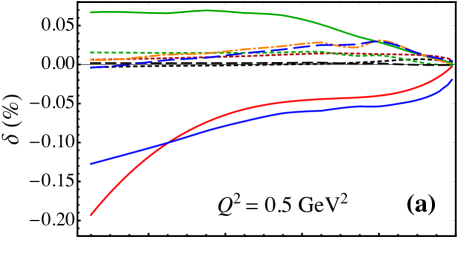
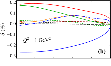
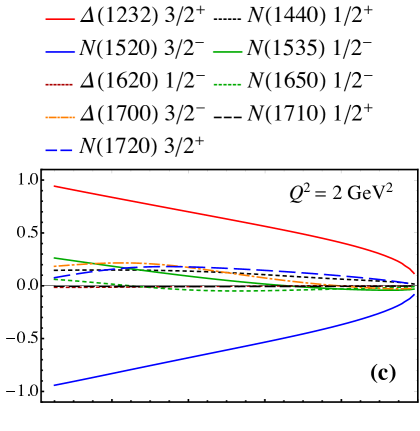
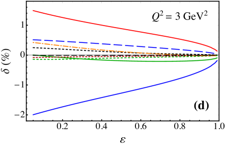
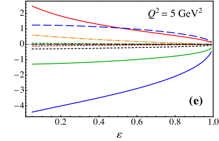
Figure 2: Relative contributions $\delta$ (in percent) to the TPE cross section for the nine spin-1/2 and spin-3/2 nucleon and $\Delta$ intermediate state resonances, as indicated in the legend, versus the virtual photon polarization $\varepsilon$ for fixed $Q^{2}$ values: (a) 0.5 GeV², (b) 1 GeV², (c) 2 GeV², (d) 3 GeV² and (e) 5 GeV². Note the vertical scale is different in each panel.

In the low-$Q^{2}$ region, for $Q^{2}$ up to $\sim 1$ GeV², the $N(1520)~{}\!3/2^{-}$ and $N(1535)~{}\!1/2^{-}$ resonances give the most significant contributions, aside from the $\Delta(1232)~{}\!3/2^{+}$ resonance, although the largest correction from the $\Delta(1232)~{}\!3/2^{+}$ ranges within only $0.2\%$ of the Born level cross section. We find an almost complete cancellation of the $N(1520)~{}\!3/2^{-}$ state contribution by that from the sum of other higher-mass resonances, leaving a net correction that is well approximated by that from the $\Delta(1232)~{}\!3/2^{+}$ alone. In this $Q^{2}$ range the $\Delta(1232)~{}\!3/2^{+}$ contribution flips in sign and suppresses the elastic nucleon intermediate state correction. At higher $Q^{2}$ values, $Q^{2}\gtrsim 2$ GeV², the $N(1520)~{}\!3/2^{-}$ overtakes the $\Delta(1232)~{}\!3/2^{+}$ contribution to $\delta$, but with opposite sign. Moreover, in the high-$Q^{2}$ region the $N(1535)~{}\!1/2^{-}$ contribution flips sign from positive to negative, however, this effect is somewhat negated by the growth of the $N(1720)~{}\!3/2^{+}$ and $\Delta(1700)~{}\!3/2^{-}$ corrections. The overall effect is that the suppression of the TPE cross section (relative to the nucleon elastic contribution) by the $\Delta(1232)~{}\!3/2^{+}$ is largely nullified by the $N(1520)~{}\!3/2^{-}$, leaving a small increase in the total TPE correction over that from the nucleon intermediate state alone.

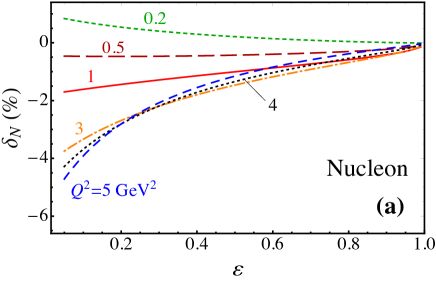
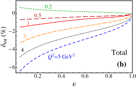
Figure 3: Contributions to the TPE correction $\delta$ (in %) versus the virtual photon polarization $\varepsilon$ for (a) nucleon only and (b) all spin-parity $1/2^{\pm}$ and $3/2^{\pm}$ states including the nucleon, at $Q^{2}=0.2$ GeV² (green dashed line), 0.5 GeV² (dark red long-dashed), 1 GeV² (red solid), 3 GeV² (orange dot-dashed), and 5 GeV² (blue dashed).

The combined effect on the TPE correction $\delta$ from all the spin-parity $1/2^{\pm}$ and $3/2^{\pm}$ resonances is illustrated in Fig. 3 as a function of virtual photon polarization, $\varepsilon$, for a range of fixed $Q^{2}$ values between 0.2 and 5 GeV². For contrast, the contribution from the nucleon elastic intermediate state alone is also shown at the same kinematics. At low $Q^{2}$ the excited state resonance contributions are found to be negligible, and the total correction is dominated by the nucleon elastic intermediate state. Note that the elastic contribution is positive at the lowest $Q^{2}$, $Q^{2}=0.2$ GeV², but rapidly changes sign and becomes increasingly more negative at higher $Q^{2}$. At $Q^{2}=5$ GeV² the nucleon contribution becomes as large as $4\%-5\%$ at low values of $\varepsilon\approx 0.1-0.2$. There is also a trend toward increasing nonlinearity at higher $Q^{2}$ values, $Q^{2}\gtrsim 3$ GeV², especially at low $\varepsilon$.

The net effect of the higher mass resonances is to increase the magnitude of the TPE correction at $Q^{2}\gtrsim 3$ GeV², due primarily to the growth of the (negative) odd-parity $N(1520)~{}\!3/2^{-}$ and $N(1535)~{}\!1/2^{-}$ resonances which overcompensates the (positive) contributions from the $\Delta(1232)~{}\!3/2^{+}$. At the highest $Q^{2}=5$ GeV² value shown in Fig. 3, the total TPE correction $\delta_{\rm tot}$ reaches $\approx$ 6-7% at low $\varepsilon$.

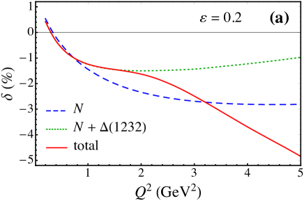
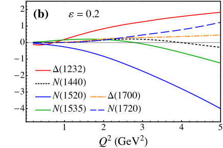
Figure 4: Contributions to the TPE correction $\delta$ (in %) versus $Q^{2}$ at backward scattering angles, $\varepsilon=0$, for (a) nucleon only (blue dashed), $N+\Delta(1232)$ (green dotted) and the sum of all resonances (red solid), and (b) the major individual contributors at the same kinematics, including the $\Delta(1232)$ (red solid), $N(1440)$ (black dashed), $N(1520)$ (blue solid), $N(1535)$ (green solid), $\Delta(1700)$ (orange dot-dashed), and $N(1720)$ (blue dashed).

To provide a more graphic illustration of the $Q^{2}$ dependence of the intermediate state resonance contributions to the cross section, we show in Fig. 4 the TPE corrections from the major individual contributors for $Q^{2}$ up to 5 GeV². We choose a nominal value for the virtual photon polarization of $\varepsilon=0.2$ in order to emphasize the largest effect on $\delta$ at backward angles. One of the prominent effects is the cancellation of part of the nucleon elastic contribution by the $\Delta(1232)~{}\!3/2^{+}$ resonance across the entire $Q^{2}$ range. On the other hand, the sum of the higher-mass resonances has a mixed impact on $\delta$. In the low-$Q^{2}$ region, $Q^{2}\lesssim 1.8$ GeV², the higher resonance state corrections largely cancel, leaving an approximately zero net contribution. As $Q^{2}$ increases, the role of the $\Delta(1232)~{}\!3/2^{+}$ is partially nullified by contributions from the higher mass resonances, and eventually is outweighed by the heavier states. An overall increase in the total TPE cross section over that from the nucleon alone is thus observed for $Q^{2}\gtrsim 3$ GeV².

In the low-$Q^{2}$ range, the odd parity $N(1520)~{}\!3/2^{-}$ resonance state gives a comparable cross section to that from the $\Delta(1232)~{}\!3/2^{+}$ state, but with opposite sign. The TPE correction from the $N(1520)~{}\!3/2^{-}$ state keeps rising with $Q^{2}$ and becomes the largest contributor at $Q^{2}\gtrsim 4$ GeV², outweighing even the elastic nucleon component. The other resonances largely cancel each other, leaving behind a negligible net contribution.

As noted previously, for the default numerical calculations presented here the resonance width has been taken to be the constant total decay width, $\Gamma_{R}$, for each resonance $R$. To explore the sensitivity of the TPE corrections to the assumptions about the width, in the next section we consider other cases, including the zero-width approximation and an energy-dependant dynamical-width.

IV.2 Nonzero resonance widths

As discussed in Sec. III.3 above, the discontinuity in the imaginary part of the TPE amplitude for the case of zero-width resonances gives rise to cusps in the real part of the amplitude from physical threshold effects at specific kinematics. In this section we consider the threshold effect on the TPE correction for the three representative resonance states $\Delta(1232)~{}\!3/2^{+}$, $N(1520)~{}\!3/2^{-}$ and $N(1720)~{}\!3/2^{+}$ discussed in Table 1.

The interplay between the resonance mass and the $Q^{2}$ and $\varepsilon$ values at which the threshold effect appears is illustrated in Fig. 5, where the TPE correction $\delta$ is shown as a function of $\varepsilon$ at several fixed values of $Q^{2}$. One observes that the higher the resonance mass, the higher the $Q^{2}$ value at which the cusp comes in. For the lowest-mass $\Delta(1232)$ excitation, the cusp at the lowest $Q^{2}=0.2$ GeV² value occurs at $\varepsilon\approx 0.06$, as indicated by the wiggle in Fig. 5(a). The effect of the constant, nonzero width, with a Breit-Wigner distribution centered at the resonance mass, is to smooth out the wiggles in the calculated $\delta$, although the effect overall is not dramatic here. At higher $Q^{2}$, above the kinematic threshold, both curves are smooth, and the finite width has little impact on the TPE correction [Fig. 5(b) and (c)].

For the intermediate-mass $N(1520)~{}\!3/2^{-}$ resonance, the effect of the kinematical threshold is more dramatic, with a prominent cusp visible for the zero-width result at $\varepsilon\approx 0.8$ for $Q^{2}=0.2$ GeV² [Fig. 5(d)], and a smaller cusp at $\varepsilon\approx 0.5$ for $Q^{2}=0.5$ GeV² [Fig. 5(e)]. In both cases the finite width of the resonance washes out the cusps, leaving a smooth function across the threshold. Above the threshold the contribution to $\delta$ is smooth [Fig. 5(f)], and the finite width has little impact. The most dramatic effect is seen for the heaviest $N(1720)~{}\!3/2^{+}$ resonance, where the kinematic threshold produces strong cusps at $\varepsilon\approx 0.9$ for $Q^{2}=0.2$ GeV² [Fig. 5(g)] and $\varepsilon\approx 0.4$ for $Q^{2}=1$ GeV² [Fig. 5(h)]. Once again the finite, constant width modulates the cusps and leads to considerably smoother results. At $Q^{2}=2$ GeV², above the kinematic threshold for this state, both the zero-width and finite-width results produce smooth curves, but the effect of the latter is still numerically significant [Fig. 5(i)].

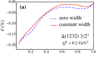
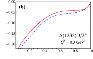
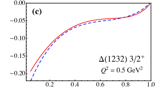
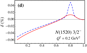
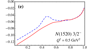
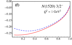
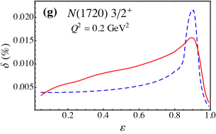
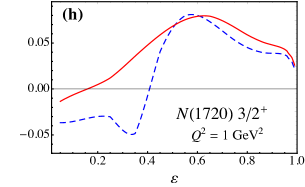
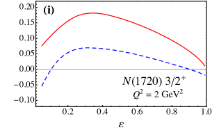
Figure 5: Effect of a finite resonance width on the TPE correction $\delta$ (in %) from three significant resonance intermediate states, $\Delta(1232)~{}\!3/2^{+}$ [(a)–(c)], $N(1520)~{}\!3/2^{-}$ [(d)–(f)], and $N(1720)~{}\!3/2^{+}$ [(g)–(i)], as a function of $\varepsilon$ at fixed $Q^{2}$ values. The kinematical kinks in the zero-width results (blue dashed lines) are smoothed out by the effect of the nonzero, constant width (red solid lines).

To test the model dependence of the TPE correction on the resonance width prescription, we also consider the effect of including an energy-dependent dynamic decay width, $\Gamma(W)$, of Eq. (50) for each resonant intermediate state. We consider the energy-dependant $\Gamma(W)$ to have contributions from three different decay channels for each resonances, namely, $\pi N$, $\pi\pi N$ and $\eta N$,

$$\Gamma(W)=\Gamma_{\pi N}(W)+\Gamma_{\pi\pi N}(W)+\Gamma_{\eta N}(W).$$ (52)

Following Ref. Hiller Blin et al. (2019), the partial decay widths $\Gamma_{\pi(\eta)N}(W)$ and $\Gamma_{\pi\pi N}(W)$ are parameterized as

$$\Gamma_{\pi(\eta)N}(W) = \Gamma_{R}\,\beta_{\pi(\eta)N}\left(\dfrac{p_{\pi(\eta)}(W)}{p_{\pi(\eta)}(W_{R})}\right)^{2L_{R}+1}\left(\dfrac{X^{2}+p_{\pi(\eta)}^{2}(W_{R})}{X^{2}+p_{\pi(\eta)}^{2}(W)}\right)^{L_{R}},$$ (53a)

$$\Gamma_{\pi\pi N}(W) = \Gamma_{R}\,\beta_{\pi\pi N}\left(\dfrac{p_{\pi\pi}(W)}{p_{\pi\pi}(W_{R})}\right)^{2L_{R}+4}\left(\dfrac{X^{2}+p_{\pi\pi}^{2}(W_{R})}{X^{2}+p_{\pi\pi}^{2}(W)}\right)^{L_{R}+2},$$ (53b)

where the constant total decay width $\Gamma_{R}$ of each resonance state is taken from Ref. Hiller Blin et al. (2019), and we have assumed the centrifugal barrier penetration factors to be the major contributors to the off-shell behavior of the resonances. Here the energy and momentum factors for the two-body channels are given by

$$p_{\pi(\eta)}(W) = \sqrt{E_{\pi(\eta)}^{2}(W)-m_{\pi(\eta)}^{2}},$$ (54a)

$$E_{\pi(\eta)}(W) = \dfrac{W^{2}+m_{\pi(\eta)}^{2}-M^{2}}{2W},$$ (54b)

and for the three-body channel is given by

$$p_{\pi\pi}(W) = \sqrt{E_{\pi\pi}^{2}(W)-4m_{\pi}^{2}},$$ (55a)

$$E_{\pi\pi}(W) = \dfrac{W^{2}+4m_{\pi}^{2}-M^{2}}{2W},$$ (55b)

where $m_{\pi(\eta)}$ is the mass of pion ($\eta$ meson). The branching fractions for the resonance decays into the $\pi N$, $\pi\pi N$ and $\eta N$ channels are given by $\beta_{\pi N}$, $\beta_{\pi\pi N}$ and $\beta_{\eta N}$, respectively, and satisfy the relation $\beta_{\pi N}+\beta_{\pi\pi N}+\beta_{\eta N}=1$. The values of the other parameters in Eqs. (53) — $X$, $L_{R}$, $\beta_{\pi N}$, $\beta_{\pi\pi N}$ and $\beta_{\eta N}$ — are taken from Ref. Hiller Blin et al. (2019).

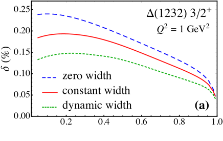
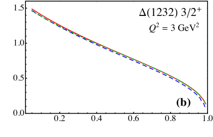
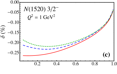
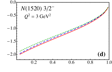
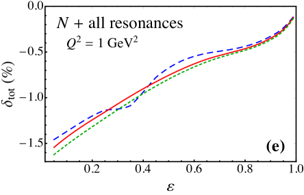
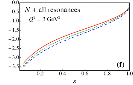
Figure 6: Comparison of the TPE correction $\delta$ (in %) computed for resonances with zero width (blue dashed lines), constant width (red solid lines) and a dynamical width (green dotted lines) for $Q^{2}=1$ GeV² (left panels) and 3 GeV² (right panels). Contributions from the $\Delta(1232)~{}\!3/2^{+}$ [(a), (b)] and $N(1520)~{}\!3/2^{-}$ [(c), (d)] states are shown separately, along with the sum of all resonance contributions [(e), (f)].

To illustrate the effect of the dynamical width, we select the two major resonance contributors to the total cross section, namely, the $\Delta(1232)~{}\!3/2^{+}$ and $N(1520)~{}\!3/2^{-}$ states. In Fig. 6(a)-(d) we compare the TPE correction $\delta$ using the dynamic, energy-dependent width with the results of the zero-width and constant-width calculations at fixed $Q^{2}=1$ and 3 GeV². At the higher $Q^{2}=3$ GeV² value, well above the kinematic thresholds, the dependence on the prescription for the width is negligibly small, with the dynamic- and constant-width results very similar to those for the zero-width case. On the other hand, at $Q^{2}=1$ GeV² the details of the treatment of the widths are more important. In particular, for the $\Delta(1232)~{}\!3/2^{+}$ the dynamical width leads to an $\approx 30\%$ reduction of the (positive) correction relative to the zero-width case across all $\varepsilon$, and a smaller but non-negligible increase in the (negative) $N(1520)~{}\!3/2^{-}$ contribution at backward angles.

For the higher-mass resonances, the contributions again enter with oscillating signs, producing a net effect of the width in the total TPE cross section ratio $\delta_{\rm tot}$, including nucleon elastic and all excited resonance states, that is very small across all $\varepsilon$ values for both $Q^{2}=1$ and 3 GeV² [Fig. 6(e)-(f)] for all three width prescriptions. The kink in the zero-width result at $\varepsilon\approx 0.4$ for $Q^{2}=1$ GeV² arises from threshold effects in the third resonance region [see Table 1 and Fig. 5(h)]. As for the $\Delta(1232)$ and $N(1520)$, the kink is eliminated by the tail effects of the resonances for either the constant-width or dynamical-width approximation, producing a smooth, monotonic result. At the higher $Q^{2}=3$ GeV² value the effects of the finite widths are negligible. Since the differences between the constant- and dynamical-width results are generally not large, for computational simplicity we employ the constant decay width approximation as the default throughout this work.

IV.3 Spin, isospin and parity dependence

To further investigate the systematics of the TPE corrections from various intermediate states resonances, we compare the relative contributions from resonances with similar spin $J$, isospin $I$ and parity $P$. In Fig. 7 we show the combined effects of the different groupings versus $Q^{2}$ for two representative values of $\varepsilon$, where the TPE effects are relatively large (backward angles, $\varepsilon=0.2$) and where they are relatively small (forward angles, $\varepsilon=0.9$). To contrast the impact of the exicted states, we show the resonance contributions separately from the nucleon elastic channel and the total (both of which are the same in the left and right columns).

For the resonance contributions with different spin, Fig. 7(a)-(b) shows qualitatively similar effects from excited states with spin $J=1/2$ and those with spin $J=3/2$. The sum of the resonances in both channels is significantly smaller than the nucleon elastic at low values of $Q^{2}$, and only starts to become non-negligible for larger $Q^{2}$, $Q^{2}\gtrsim(3-4)$ GeV², with the relative impact somewhat greater at high $\varepsilon$ than at low $\varepsilon$. The total TPE correction $\delta$ is therefore well approximated by the elastic term alone for $Q^{2}\lesssim 3$ GeV² at $\varepsilon=0.2$ and $Q^{2}\lesssim 2$ GeV² at $\varepsilon=0.9$.

The decomposition into contributions from different isospins in Fig. 7(c)-(d) is rather more dramatic. Large cancellations occur between the (negative) isospin $I=1/2$ intermediate states and the (positive) $I=3/2$ states. At lower $Q^{2}$, $Q^{2}\lesssim 2$ GeV², the $I=3/2$ transitions are dominant, while at larger $Q^{2}$ the $I=1/2$ intermediate states become more important, rendering the TPE effect more negative compared with the nucleon elastic term alone and contributing to the rapid increase in magnitude of the (negative) total TPE correction with $Q^{2}$. This qualitative behavior is similar at low and high $\varepsilon$.

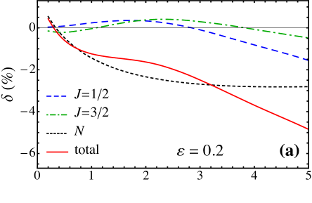
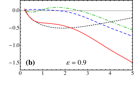
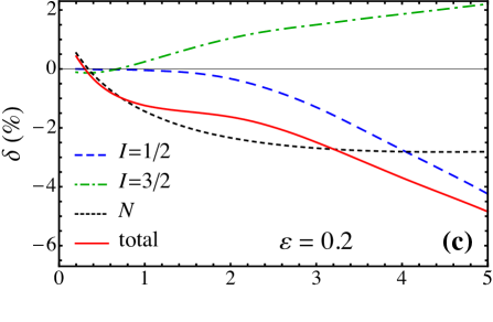
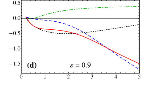
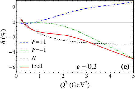
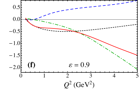
Figure 7: Comparison between the contributions to the TPE correction $\delta$ (in %) from intermediate state resonances with spin $J=1/2$ and $J=3/2$ [(a), (b)], isospin $I=1/2$ and $I=3/2$ [(c), (d)], and even parity $P=+1$ and odd parity $P=-1$ [(e), (f)], for $\varepsilon=0.2$ (left columns) and $\varepsilon=0.9$ (right columns). The nucleon-only contribution (black dotted lines), which is not included in the other curves, and the total (red solid lines) are shown for comparison in each panel.

Interestingly, a similar cancellation is found between the parity-even ($P=+1$) and parity-odd ($P=-1$) intermediate states in Fig. 7(e)-(f). In this case the $P=+1$ contributions to $\delta$ are positive while the $P=-1$ contributions are negative, with the latter becoming more important with increasing $Q^{2}$. The qualitative behavior of the curves for each of the spin, isospin and parity decompositions can be understood from the results illustrated in Fig. 2, where numerically the largest positive contribution is seen to be from the $\Delta(1232)~{}\!3/2^{+}$ and the negative of that from $N(1520)~{}\!3/2^{-}$ states. The former dominates the isospin 3/2 and even-parity channels, while the latter dominates the isospin 1/2 and odd-parity channels, but since both have spin 3/2 and enter with opposite signs, their combined contributions largely cancel, leaving the spin-1/2 channel as the relatively more important one phenomenologically.

IV.4 Generalized TPE form factors

Before proceeding to the quantitative comparison of the calculated full cross sections with experimental observables sensitive to TPE effects, in this section we present the TPE results in terms of the generalized TPE form factors introduced in Sec. III.3.1. In Fig. 8 we present the $\varepsilon$ dependence of the TPE form factors $F^{\prime}_{1}$, $F^{\prime}_{2}$ and $G^{\prime}_{a}$ at fixed values of $Q^{2}=1$ GeV² and 5 GeV², scaled by a dipole form factor $G_{D}$,

$$G_{D}(Q^{2}) = \bigg{(}\frac{\Lambda^{2}}{Q^{2}+\Lambda^{2}}\bigg{)}^{2}\ ,$$ (56)

with mass $\Lambda=0.84$ GeV. Illustrated are the individual contributions from the nucleon elastic intermediate state and the 3 most prominent resonance states, namely, the $\Delta(1232)~{}\!3/2^{+}$, $N(1520)~{}\!3/2^{-}$, and the $N(1720)~{}\!3/2^{+}$, as well as the total.

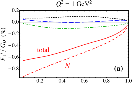
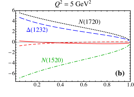
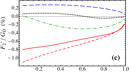
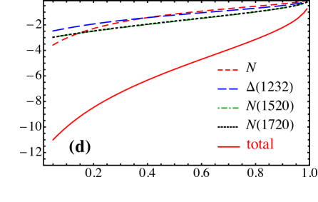
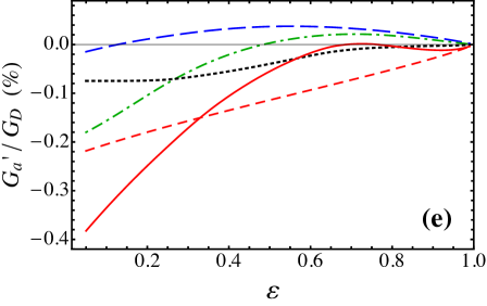
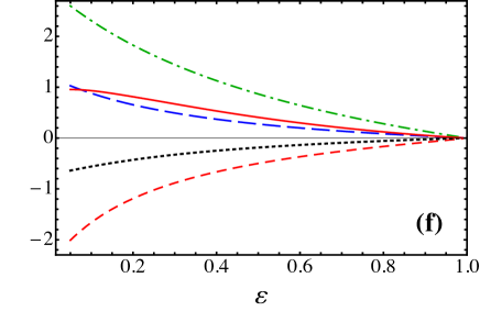
Figure 8: Generalized TPE form factors $F^{\prime}_{1}$ [(a), (b)], $F^{\prime}_{2}$ [(c), (d)], and $G^{\prime}_{a}$ [(e), (f)], scaled by the dipole form factor $G_{D}$, versus $\varepsilon$ at fixed $Q^{2}=1$ GeV² (left column) and 5 GeV² (right column) for the nucleon elastic (red dashed lines), $\Delta(1232)~{}\!3/2^{+}$ (blue long-dashed lines), $N(1520)~{}\!3/2^{-}$ (green dot-dashed lines), $N(1720)~{}\!3/2^{+}$ (black dotted lines), and total TPE (red solid lines) contributions.

Clearly evident for the $F_{1}^{\prime}$ TPE form factor is that at $Q^{2}=1$ GeV² this contribution is negative at all $\varepsilon$ values and is dominated by the nucleon elastic state. The higher-mass resonance contributions grow rapidly with increasing $Q^{2}$, but there is a strong cancellation between the (positive) $J^{P}=3/2^{+}$ and (negative) $J^{P}=3/2^{-}$ states, rendering the total effect to be very small and close to zero at $Q^{2}=5$ GeV².

For the Pauli $F_{2}^{\prime}$ TPE form factor, a similar pattern repeats as for the Dirac form factor, namely, at $Q^{2}=1$ GeV² the cancellations between the various resonance contributions leave the total TPE form factor to be negative and dominated by the nucleon elastic intermediate state. In contrast to the $F_{1}^{\prime}$ case, however, at larger $Q^{2}$ the main resonance contributions grow in magnitude but remain negative, so that the net effect is a coherent enhancement of the TPE form factor up to $\sim 10\%$ of the dipole at $Q^{2}=5$ GeV² for backward angles.

For the axial $G^{\prime}_{a}$ TPE form factor, the magnitude of the various resonance contributions is generally smaller than for the other two TPE form factors, with the nucleon elastic state giving negative contributions at both low and high $Q^{2}$. Once again a high degree of cancellation occurs between the (positive) $\Delta(1232)$ and $N(1520)$ states and the (negative) nucleon elastic and $N(1720)$ states, leaving an overall small positive total correction to $G^{\prime}_{a}$.

In fact, as observed by Borisyuk and Kobushkin Borisyuk and Kobushkin (2008), it is quite natural to combine the small $G^{\prime}_{a}$ contribution with the $F^{\prime}_{1}+F^{\prime}_{2}$ form factor combination into an effective “magnetic” TPE form factor ${\cal G}_{M}$ as in Eq. (43b). Observing that the TPE FFs in Fig. 8 do not in general show strong variation with $\varepsilon$, in Fig. 9 we display the $Q^{2}$ dependence of both the “electric” and “magnetic” TPE form factor ${\cal G}_{E}$ and ${\cal G}_{M}$, scaled by the dipole form factors, at a fixed value of $\varepsilon=0.2$, where the TPE effects are not suppressed.

For $Q^{2}\gtrsim 2$ GeV² one observes that the magnitude of both the generalized electric ${\cal G}_{E}$ and magnetic ${\cal G}_{M}$ TPE form factors rises linearly with $Q^{2}$. The positive sign of ${\cal G}_{E}$ and the negative sign of ${\cal G}_{M}$ result in corrections to the effective Born level form factors that render the $G_{E}/G_{M}$ ratio smaller than that naively extracted from cross section data without TPE corrections. This would make it more compatible with the $G_{E}/G_{M}$ ratio extracted from the polarization transfer data, which suggest a strong fall-off of the ratio with $Q^{2}$ above $Q^{2}\sim 1$ GeV², resolving the discrepancy with the Rosenbluth cross section results.

At low $Q^{2}$, $Q^{2}\lesssim 1$ GeV², the TPE form factors are dominated by the nucleon elastic contribution, as already indicated in the $Q^{2}$ dependence of the total TPE correction $\delta$ in Fig. 4. For higher $Q^{2}$ values, $Q^{2}\gtrsim 2$ GeV², the magnitudes of the various excited state contributions grow, with the $\Delta(1232)$ and $N(1720)$ contributions to both ${\cal G}_{E}$ and ${\cal G}_{M}$ remaining positive and the $N(1520)$ states negative.

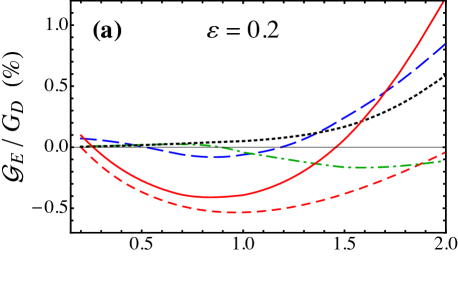
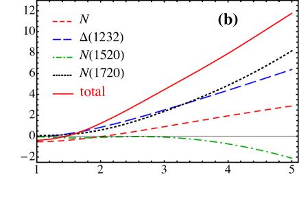
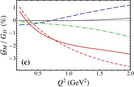
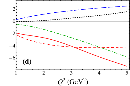
Figure 9: Generalized TPE form factors ${\cal G}_{E}$ [(a), (b)] and ${\cal G}_{M}$ [(c), (d)], scaled by the dipole form factor $G_{D}$, at fixed $\varepsilon=0.2$ for low $Q^{2}$ ($Q^{2}\leq 2$ GeV², left column) and high $Q^{2}$ ($1\leq Q^{2}\leq 5$ GeV², right column), for the nucleon elastic (red dashed lines), $\Delta(1232)~{}\!3/2^{+}$ (blue long-dashed lines), $N(1520)~{}\!3/2^{-}$ (green dot-dashed lines), $N(1720)~{}\!3/2^{+}$ (black dotted lines), and total TPE (red solid lines) contributions.

More specifically, while the $N(1520)$ resonance state gives rather small corrections to ${\cal G}_{E}$ at most values of $Q^{2}$, its contribution to ${\cal G}_{M}$ becomes even more important than the nucleon elastic for the largest $Q^{2}$, $Q^{2}\gtrsim 4$ GeV². Because of the $\tau$ factor in Eq. (44), the magnetic contribution to the total cross section dominates at high $Q^{2}$, so that the $N(1520)$ state plays the most significant role in the TPE cross section at high $Q^{2}$. At high $Q^{2}$ the negative sign of the ${\cal G}_{M}$ TPE form factor is driven by the nucleon elastic and $N(1520)$ states, while the positive sign of the ${\cal G}_{E}$ TPE form factor is due mostly to the $\Delta(1232)$ and $N(1720)$.

V TPE-sensitive observables

Having described the features of the TPE corrections from excited intermediate states to elastic $ep$ scattering cross sections in the previous sections, in the remainder of this paper we will discuss the impact of these corrections on observables sensitive to the TPE effects. In particular, we analyze the numerical effects of the calculated TPE corrections on the elastic $e^{+}p$ to $e^{-}p$ cross section ratio measured recently by the CLAS Rimal et al. (2017), VEPP-3 Rachek et al. (2015) and OLYMPUS Henderson et al. (2017) experiments, as well as with polarization transfer data from the GEp$2\gamma$ experiment Meziane et al. (2011) in Hall C at Jefferson Lab. In addition, we investigate the effect of the resonance contributions to the TPE on the proton $G_{E}/G_{M}$ form factor ratio discrepancy between the LT and PT data Blunden et al. (2003, 2005); Guichon and Vanderhaeghen (2003); Chen et al. (2004).

V.1 $e^{+}p$ to $e^{-}p$ elastic scattering ratio

Perhaps the most direct consequence of TPE in lepton scattering is the deviation from unity of the ratio of $e^{+}p$ to $e^{-}p$ elastic scattering cross sections. The interference of the Born amplitude and the TPE amplitude here depends on the sign of the lepton charge, so that the ratio

$$R_{2\gamma}\ =\ \frac{\sigma(e^{+}p)}{\sigma(e^{-}p)}\ \approx\ 1-2\,\delta_{\gamma\gamma},$$ (57)

where $\sigma(e^{\pm}p)\equiv d\sigma(e^{\pm}p\to e^{\pm}p)/d\Omega$, is a direct measure of the TPE correction $\delta_{\gamma\gamma}$. Early measurements of $R_{2\gamma}$ in the 1960s at SLAC Browman et al. (1965); Mar et al. (1968), Cornell Anderson et al. (1966), DESY Bartel et al. (1967) and Orsay Bouquet et al. (1968) obtained some hints of nonzero TPE effects, however, since the data were predominantly at low $Q^{2}$ and forward angles the deviations of $R_{2\gamma}$ from unity were small and within the experimental uncertainties. The more recent experiments at Jefferson Lab Rimal et al. (2017), Novosibirsk Rachek et al. (2015) and DESY Henderson et al. (2017) have attempted more precise determinations of $R_{2\gamma}$ over a larger range of $Q^{2}$ and $\varepsilon$ values than previously available.

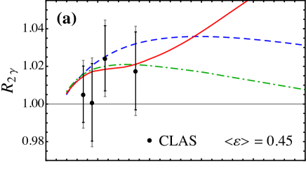
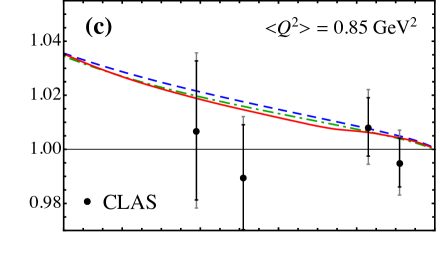
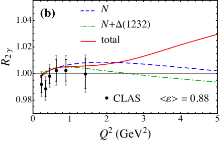
Figure 10: Ratio $R_{2\gamma}$ of $e^{+}p$ to $e^{-}p$ elastic cross sections from CLAS Rimal et al. (2017) (a) versus $Q^{2}$ for fixed averaged $\langle\varepsilon\rangle=0.45$ and (b) $\langle\varepsilon\rangle=0.88$, (c) versus $\varepsilon$ for fixed averaged $\langle Q^{2}\rangle=0.85$ GeV² and (d) $\langle Q^{2}\rangle=1.45$ GeV², compared with the nucleon only (blue dashed lines), sum of nucleon and $\Delta(1232)$ (green dot-dashed lines), and sum of all intermediate state contributions (red solid lines). The experimental statistical and systematic uncertainties are indicated by the (black) inner and (gray) outer error bars, respectively.

The $R_{2\gamma}$ ratio from the CLAS experiment Rimal et al. (2017) is shown in Fig. 10 versus $Q^{2}$ at fixed averaged $\varepsilon$ values, $\langle\varepsilon\rangle=0.45$ and 0.88 [Fig. 10(a), (b)], and versus $\varepsilon$ for fixed averaged $Q^{2}$, $\langle Q^{2}\rangle=0.85$ and 1.45 GeV² [Fig. 10(c), (d)]. The deviations from unity of the measured ratios are relatively small, with most of the data points consistent with no TPE effects within the relatively large experimental uncertainties. (Note that in Fig. 10 and in subsequent data comparisons, the statistical and systematic uncertainties are shown separately as inner and outer error bars, respectively.) The data are also consistent, however, with the calculated TPE corrections, which are $\lesssim 2\%$ in the measured region, but increase at lower $\varepsilon$ and higher $Q^{2}$. A significant contribution to the cross section ratio is observed from the nucleon elastic intermediate state, with the $\Delta(1232)~{}\!3/2^{+}$ resonance canceling some of the deviation from unity. The higher mass resonances have little impact in the experimentally measured regions of $\varepsilon$ and $Q^{2}$, but their contributions become more significant at higher $Q^{2}$ in particular, $Q^{2}\gtrsim 3$ GeV².

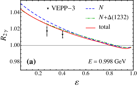
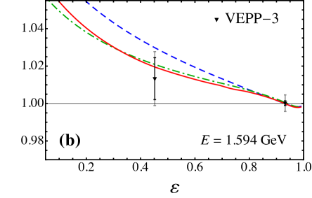
Figure 11: Ratio $R_{2\gamma}$ of $e^{+}p$ to $e^{-}p$ elastic cross sections versus $\varepsilon$ from the VEPP-3 experiment Rachek et al. (2015) for beam energy (a) $E=0.998$ GeV and (b) $E=1.594$ GeV, compared with the nucleon only (blue dashed lines), sum of nucleon and $\Delta(1232)$ (green dot-dashed lines), and sum of all intermediate state contributions (red solid lines). The experimental statistical and systematic uncertainties are indicated by the (black) inner and (gray) outer error bars, respectively.

A similar comparison of the calculated $R_{2\gamma}$ ratio with data from the VEPP-3 experiment at Novosibirsk Rachek et al. (2015) is shown in Fig. 11. The experiment scattered electrons at fixed beam energy $E=0.998$ GeV [Fig. 11(a)] and $E=1.594$ GeV [Fig. 11(b)], for $\varepsilon$ down to $\approx 0.3$. This corresponds to a $Q^{2}$ range between $\approx 0.3$ GeV² and 1.5 GeV². At these $Q^{2}$ values the nucleon elastic intermediate state gives the largest contribution, with again the $\Delta(1232)$ canceling some of the effect, and bringing the calculation with the TPE corrections in better agreement with the data. The contributions of the higher mass resonances at the kinematics of this experiment are negligible.

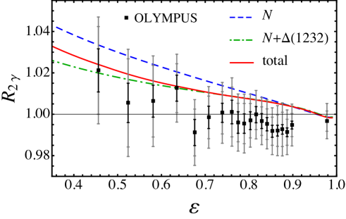
Figure 12: Ratio $R_{2\gamma}$ of $e^{+}p$ to $e^{-}p$ elastic cross sections versus $\varepsilon$ from the OLYMPUS experiment Henderson et al. (2017) with beam energy $E=2.01$ GeV, compared with the nucleon only (blue dashed lines), sum of nucleon and $\Delta(1232)$ (green dot-dashed lines), and sum of all intermediate state contributions (red solid lines). The experimental statistical and systematic uncertainties are indicated by the (black) inner and (gray) outer error bars, respectively.

The most recent OLYMPUS experiment at DESY Henderson et al. (2017) measured the ratio $R_{2\gamma}$ over a range of $\varepsilon$ from $\approx 0.46$ to 0.9 at an electron energy $E\approx 2$ GeV, with $Q^{2}$ ranging up to $\approx 2$ GeV². The results, illustrated in Fig. 12, indicate an enhancement of the ratio at $\varepsilon\lesssim 0.6$ and a dip below unity at $\varepsilon\gtrsim 0.7$, although still compatible with no deviation from 1 within the combined statistical and systematic uncertainties. The suppression of the ratio at large $\varepsilon$ is in slight tension from other measurements, but again the effect is consistent within the errors Blunden and Melnitchouk (2017). Inclusion of the $\Delta(1232)$ intermediate state reduces the effect of the nucleon elastic contribution away from the forward scattering region, but the effect of the higher mass resonances is very small for all $\varepsilon$ shown. The overall agreement between the TPE calculation and the OLYMPUS data is reasonable within the experimental uncertainties, although there is no indication in our model for a decrease of the ratio below unity at large $\varepsilon$.

V.2 Polarization observables

In addition to the unpolarized $e^{+}p$ to $e^{-}p$ cross section ratio, other observables that are directly sensitive to the presence of effects beyond the Born approximation involve elastic scattering of longitudinally polarized electrons from unpolarized protons, with polarization transferred to the final state proton, $\vec{e}\,p\to e\,\vec{p}$. The relevant observables are the transverse and longitudinal polarizations, $P_{T}$ and $P_{L}$, defined relative to the proton momentum in the scattering plane as

$$P_{T} = -\dfrac{\sqrt{2\tau\varepsilon(1-\varepsilon)}}{\sigma_{R}}\left[G_{E}G_{M}+G_{M}\operatorname{Re}{\cal G}_{E}+G_{E}\operatorname{Re}\Big{(}{\cal G}_{M}+\dfrac{\nu\varepsilon}{\tau}G_{a}^{\prime}\Big{)}\right],$$ (58a)

$$P_{L} = \dfrac{\tau\sqrt{1-\varepsilon^{2}}}{\sigma_{R}}\left[G_{M}^{2}+2G_{M}\operatorname{Re}\Big{(}{\cal G}_{M}+\dfrac{\nu\varepsilon^{2}}{\tau(1+\varepsilon)}G^{\prime}_{a}\Big{)}\right],$$ (58b)

where $\sigma_{R}=\sigma_{R}^{\rm Born}(1+\delta_{\gamma\gamma})$, and the reduced Born cross section $\sigma_{R}^{\rm Born}$ is given in Eq. (6). The ratio of the transverse to longitudinal polarizations is then given by

$$R_{TL}=-\mu_{p}\sqrt{\dfrac{\tau(1+\varepsilon)}{2\varepsilon}}\dfrac{P_{T}}{P_{L}}.$$ (59)

In the Born approximation, $R_{TL}$ reduces to the ratio of electric to magnetic form factors, $\mu_{p}G_{E}/G_{M}$, and becomes independent of $\varepsilon$. Any observed $\varepsilon$ dependence of $R_{TL}$ would therefore be an indication of TPE effects.

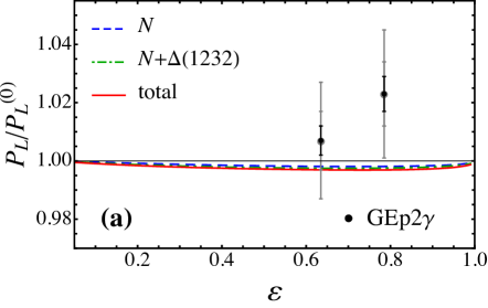
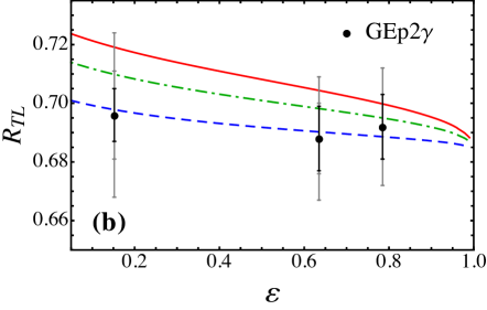
Figure 13: Effect of TPE corrections on polarization observables from the GEp2$\gamma$ experiment at Jefferson Lab Meziane et al. (2011) for (a) longitudinal polarization $P_{L}$ relative to the Born level result $P_{L}^{(0)}$, and (b) polarization transfer ratio $R_{TL}$ at $Q^{2}=2.49$ GeV², compared with calculations including nucleon only (blue dashed lines), sum of nucleon and $\Delta(1232)$ (green dot-dashed lines), and sum of all intermediate state contributions (red solid lines). The experimental statistical and systematic uncertainties are indicated by the (black) inner and (gray) outer error bars, respectively.

Data on the transverse and longitudinal polarizations were obtained from the GEp_2γ experiment at Jefferson Lab Meziane et al. (2011), and are shown in Fig. 13 for the ratio $P_{L}/P_{L}^{(0)}$, where $P_{L}^{(0)}$ is the Born level longitudinal polarization, and the ratio $R_{TL}$ versus $\varepsilon$ at an average value of $Q^{2}=2.49$ GeV². The calculated TPE effect in our model is almost negligible for the longitudinal polarization, giving very little additional $\varepsilon$ dependence in the ratio $P_{L}/P_{L}^{(0)}$ in Fig. 13(a), and consistent within 1$\sigma$ with the data. A larger TPE effect is found for the transverse polarization, where the nucleon alone gives a small slope in $\varepsilon$, with the effects of the $\Delta(1232)$ and higher mass intermediate states enhancing the TPE correction to $\approx 3\%$ effect at $\varepsilon\approx 0.2$. For the nucleon intermediate state this was already concluded in the earlier analysis in Ref. Blunden et al. (2005). The data do not show any clear evidence for an $\varepsilon$ dependence within the experimental uncertainties, although the calculated effect is also compatible with the data within 1$\sigma$ errors.

V.3 Electric to magnetic form factor ratio $\mu_{p}G_{E}/G_{M}$

Perhaps the most well-known consequence of TPE that has been identified in the last two decades is the ratio of the electric to magnetic form factors extracted from elastic scattering cross sections using the LT separation method Blunden et al. (2003). Longitudinal-transverse separation requires measurements of cross sections as a function of $\varepsilon$ (or scattering angle) at fixed values of $Q^{2}$. In the Born approximation, the reduced cross section $\sigma_{R}^{\rm Born}$ in Eq. (6) is a linear function of $\varepsilon$, which allows the form factors $G_{M}^{2}$ and $G_{E}^{2}$ to be extracted from a linear fit to the reduced cross section data.

As observed in the preceding sections, the TPE correction induces an additional shift in the $\varepsilon$ dependence, which alters the effective slope of the reduced cross section versus $\varepsilon$. Furthermore, since the $\varepsilon$ dependence of the TPE effect is not restricted to be linear, any nonlinearity introduced through radiative corrections could potentially complicate the form factor extraction via the LT analysis, especially at higher values of $Q^{2}$.

In Secs. V.1 and V.2 we compared the available data to calculations incorporating TPE effects. However, to extract $G_{E}$ and $G_{M}$ it is more appropriate to correct the data for TPE contributions at the same level as other radiative corrections in order to obtain the genuine Born contribution, $\sigma_{R}^{\rm Born}$. The measured and Born cross sections can be related by

$$\sigma_{R}^{\rm meas}\,=\,C_{\rm RC}^{\rm old}\,\left(\sigma_{R}^{\rm Born}\right)^{\rm old}\,=\,C_{\rm RC}^{\rm new}\,\left(\sigma_{R}^{\rm Born}\right)^{\rm new},$$ (60)

where $C_{\rm RC}^{\rm old}$ is the radiative correction (RC) factor applied in the original analyses Walker et al. (1994); Andivahis et al. (1994), and $C_{\rm RC}^{\rm new}$ incorporates any improvements, including the new TPE effects. For the RC factor $C_{\rm RC}$ we adopt the definition used by Gramolin and Nikolenko Gramolin and Nikolenko (2016),

$$C_{\rm RC} = C_{L}\exp\left(\delta_{\rm RC}+\delta\right),$$ (61a)

$$\delta_{\rm RC} = \delta({\rm MTj})+\delta_{\rm VP}+\delta_{\rm brems},$$ (61b)

where $C_{L}$ is the correction factor for ionization losses in the target, $\delta({\rm MTj})$ represents the standard RCs of Maximon and Tjon Maximon and Tjon (2000), $\delta_{\rm VP}$ are vacuum polarization corrections not included in $\delta({\rm MTj})$, $\delta_{\rm brems}$ are hard photon internal and external bremsstrahlung corrections not accounted for in $\delta({\rm MTj})$, and $\delta$ is the hard TPE correction $\delta=\delta_{\gamma\gamma}-\delta_{\rm IR}({\rm MTj})$ in Eq. (22). Although exponentiation is strictly only justified for the soft photon emission correction, it is conventionally applied to all RCs.

Gramolin and Nikolenko Gramolin and Nikolenko (2016) reanalyzed the SLAC data Walker et al. (1994); Andivahis et al. (1994), which used the standard RCs of Mo and Tsai Mo and Tsai (1969), to include improvements to $\delta_{\rm brems}$ as well as the use of the standard RCs of Maximon and Tjon Maximon and Tjon (2000). Their Born cross section can be written in terms of that given in Refs. Walker et al. (1994); Andivahis et al. (1994) as

$$\left(\sigma_{R}^{\rm Born}\right)^{\rm new}\,=\,\frac{C_{\rm RC}^{\rm old}}{C_{\rm RC}^{\rm new}}\left(\sigma_{R}^{\rm Born}\right)^{\rm old}.$$ (62)

The ratio $C_{\rm RC}^{\rm old}/C_{\rm RC}^{\rm new}$ is tabulated for the SLAC data in Ref. Gramolin and Nikolenko (2016), to which we add our calculated TPE contribution $\delta$. For the Super-Rosenbluth data Qattan et al. (2005) details of the RCs that were applied are not available, so the improvements made to $\delta_{\rm RC}$ are restricted to using $\delta_{\rm IR}({\rm MTj})$ instead of $\delta_{\rm IR}({\rm MTs})$.

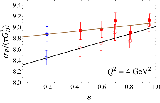
Figure 14: Reduced cross section $\sigma_{R}^{\rm Born}$ at $Q^{2}=4$ GeV², scaled by $\tau$ times the dipole form factor squared $G_{D}^{2}$. Open circles are the original data points from Ref. Andivahis et al. (1994). Filled circles (slightly offset for clarity) include improved standard RCs from Ref. Gramolin and Nikolenko (2016), together with the TPE corrections from the present work. The weighted least squares fits (solid lines) determine $G_{E}^{2}$ and $G_{M}^{2}$. Data points from the 8 GeV spectrometer are shown in red, while the data point from the 1.6 GeV spectrometer (which is separately normalized Andivahis et al. (1994)) is shown in blue.

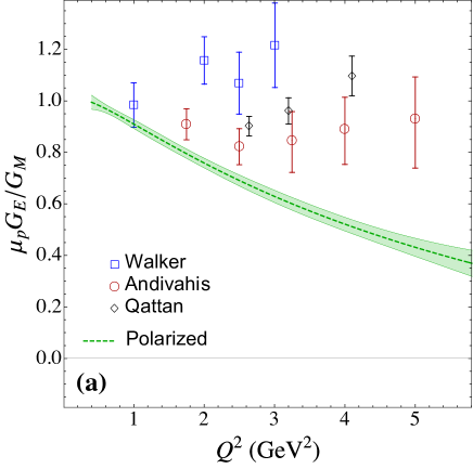
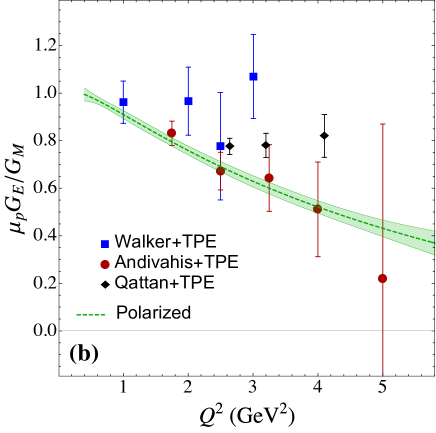
Figure 15: (a) Ratio of the proton electric to magnetic form factors, $\mu_{p}\,G_{E}/G_{M}$, versus $Q^{2}$, extracted using LT separation data Walker et al. (1994); Andivahis et al. (1994); Qattan et al. (2005). A nonlinear fit to the combined PT results Jones et al. (2000); Gayou et al. (2002); Punjabi et al. (2005); Puckett et al. (2010, 2012) at the 99% confidence limit is shown by the green band. (b) The ratio $\mu_{p}\,G_{E}/G_{M}$ extracted from a reanalysis of the LT data using improved standard RCs from Ref. Gramolin and Nikolenko (2016), together with the TPE effects from the present work.

A comparison of the original reduced cross sections and the results with the improved RCs of Ref. Gramolin and Nikolenko (2016) plus our TPE is shown in Fig. 14 for the $Q^{2}=4$ GeV² data from Ref. Andivahis et al. (1994). We note that the original and the TPE-corrected data are equally well described by a linear dependence on $\varepsilon$, and no nonlinearity effects are apparent.

In Fig. 15 we show the $G_{E}/G_{M}$ ratio extracted from our analysis for the SLAC Walker et al. (1994); Andivahis et al. (1994) and Jefferson Lab Super-Rosenbluth Qattan et al. (2005) experiments up to $Q^{2}=5$ GeV². To avoid clutter, the PT data from Refs. Jones et al. (2000); Gayou et al. (2002); Punjabi et al. (2005); Puckett et al. (2010, 2012) are shown as a band, which is a nonlinear fit at the 99% confidence limit. The original analysis, shown in Fig. 15(a), is consistent with $\mu_{p}G_{E}/G_{M}\approx 1$, while a progressively larger effect of TPE with increasing $Q^{2}$ for all LT data sets is seen in Fig. 15(b), with a commensurate increase in the uncertainty of $G_{E}$. In particular the LT data of Andivahis et al. Andivahis et al. (1994) are striking in their consistency with the PT band, with a near linear falloff of $G_{E}/G_{M}$ with $Q^{2}$. These results provide compelling evidence that there is no inconsistency between the LT and PT data once improvements in the RCs and TPE effects are made.

VI Conclusions

In this study we have applied the recently developed dispersive formalism of Ref. Blunden and Melnitchouk (2017) to compute the TPE corrections to elastic electron-proton cross sections, including for the first time contributions from all $J^{P}=1/2^{\pm}$ and $3/2^{\pm}$ excited intermediate state resonances with mass below 1.8 GeV. For the resonance electrocouplings at the hadronic vertices we employed newly extracted helicity amplitudes from the analysis of CLAS meson electroproduction data at $Q^{2}\lesssim 5$ GeV² Hiller Blin et al. (2019); Mokeev et al. (2012, 2009).

To assess the model dependence of the resonance calculations, we investigated the effects of finite Breit-Wigner resonance widths, comparing the TPE results for the pointlike, constant width and variable width approximations. We found that for the pointlike case kinematical thresholds produce artificial cusps at specific values of $Q^{2}$ and $\varepsilon$, however, these are effectively smoothed out across all kinematics when a nonzero width is introduced. The effect of using a constant or dynamical width was less dramatic, with the latter reducing somewhat the magnitude of some of the low-lying resonances, such as the $\Delta(1232)$, at low $Q^{2}\sim 1$ GeV² and at backward angles.

We also examined the spin, isospin and parity dependence of the resonance contributions to the TPE amplitudes, finding large cancellations between the (negative) isospin $I=1/2$ and the (positive) $I=3/2$ intermediate states, as well as between the parity-even and parity-odd contributions. This behavior is mostly driven by the dominance of the (positive) $\Delta(1232)~{}\!3/2^{+}$ and (negative) $N(1520)~{}\!3/2^{-}$ contributions to the TPE amplitudes, especially at larger $Q^{2}$ values.

More specifically for the individual hadronic intermediate states, at low $Q^{2}$, $Q^{2}\lesssim 1$ GeV², the nucleon elastic state dominates, with contributions from excited states there mostly negligible. For $Q^{2}\approx$ (1 – 2) GeV², the $\Delta(1232)$ resonance starts to play a more important role, and here the sum of $N+\Delta(1232)$ provides a good approximation to the total TPE amplitude. At still larger $Q^{2}$, the $N(1520)$ gives the largest contribution among the higher-mass resonances, exceeding even the nucleon component for $Q^{2}\gtrsim 4$ GeV². The higher-mass resonances each grow with increasing $Q^{2}$, but enter with different signs and largely cancel each other’s contributions. Compared to the nucleon elastic component alone, the resonance excitations give rise to an overall enhancement of the TPE cross section correction for $Q^{2}\gtrsim 3$ GeV².

The excited state resonance contributions generally provide some improvement of the phenomenological description of observables that are sensitive to TPE corrections, such as the ratios of $e^{+}p$ to $e^{-}p$ elastic cross sections measured recently in dedicated experiments at Jefferson Lab Rimal et al. (2017), Novosibirsk Rachek et al. (2015) and DESY Henderson et al. (2017). Unfortunately, most of these data are in kinematic regions where resonance contributions are not large, and in some cases the results are consistent with no TPE effect within the experimental uncertainty. On the other hand, the resolution of the $G_{E}/G_{M}$ ratio discrepancy with the inclusion of the TPE corrections, especially for the cross section data of Andivahis et al. Andivahis et al. (1994), compels a global reanalysis of the LT data with inclusion of all other radiative corrections and TPE at the same level.

Improvements on the theoretical front should involve exploration of the effects from spin-5/2 intermediate resonant states, as well as incorporation of nonresonant contributions Tomalak et al. (2017) at larger $Q^{2}$ values. Future precision measurements at higher $Q^{2}$ values and backward angles (small $\varepsilon$), where the TPE effects are expected to be most significant, would be helpful for better constraining the TPE calculations. This would provide a more complete understanding of the relevance of TPE in the resolution of the proton’s $G_{E}/G_{M}$ form factor ratio puzzle, and better elucidate the role of multi-photon effects in electron scattering in general.