A Velocity-Entropy Invariance theorem for the Chapman-Jouguet detonation

Abstract

The velocity and the specific entropy of the Chapman-Jouguet (CJ) equilibrium detonation in a homogeneous explosive are shown to be invariant under the same variation of the initial pressure and temperature. The CJ state, including its adiabatic exponent and isentrope, can then be calculated from the CJ velocity or, conversely, the CJ velocity from one CJ variable, without using an equation of state of detonation products. For gaseous explosives, the comparison to calculations with detailed chemical equilibrium shows agreement to within $\mathcal{O}(0.1)$%. However, the CJ pressures of four liquid carbon explosives are found about 20 % greater than the measurements. The CJ-equilibrium model appears not to be compatible with the velocities and the pressures measured in these explosives. A simple criterion for assessing the representativeness of this model is thus proposed, which, however, cannot indicate which of its assumptions would not be satisfied, such as chemical equilibrium or single-phase fluid. This invariance might illustrate a general feature of hyperbolic systems and their characteristic surfaces.

I Introduction

The Chapman-Jouguet (CJ) detonation [1] is a classic of the combustion theory, defined as the fully reactive, plane, and compressive discontinuity wave with a constant velocity supersonic relative to the initial state and sonic relative to the final burnt state at chemical equilibrium. The CJ state and velocity are thus calculated through the Rankine-Hugoniot (RH) relations and an equation of state of detonation products. However, detonation processes are unstable and very sensitive to losses, which the RH relations cannot describe. The CJ model only provides limiting reference velocities and reaction-end states independently of any condition for detonation existence and, as such, is the staple of detonation theory. It is the purpose of this study to bring out and investigate two supplemental CJ properties perhaps useful as a semi-empirical tool to interpret experiments and improve modelling.

The first one is that the CJ detonation velocity $D_{\text{CJ}}$ and the specific entropy $s_{\text{CJ}}$ of a homogeneous explosive substance are invariant under the same variations of the initial temperature $T_{0}$ and pressure $p_{0}$: if one is invariant, so is the other; different initial states producing the same $D_{\text{CJ}}$ produce different CJ states on the same isentrope. The second one is that a CJ state and its isentrope can then be easily calculated from the value of $D_{\text{CJ}}$ without equilibrium equation of state; conversely, $D_{\text{CJ}}$ can be obtained from one CJ variable. They apply only to explosives whose fresh and burnt states are single-phase inviscid fluids, with temperature $T$ and pressure $p$ as independent variables. Figure 1 depicts the CJ model and the Velocity-Entropy Invariance (DSI) theorem in the Pressure ($p$) - Volume ($v$) plane based on usual properties of detonation modelling (Sect. II).

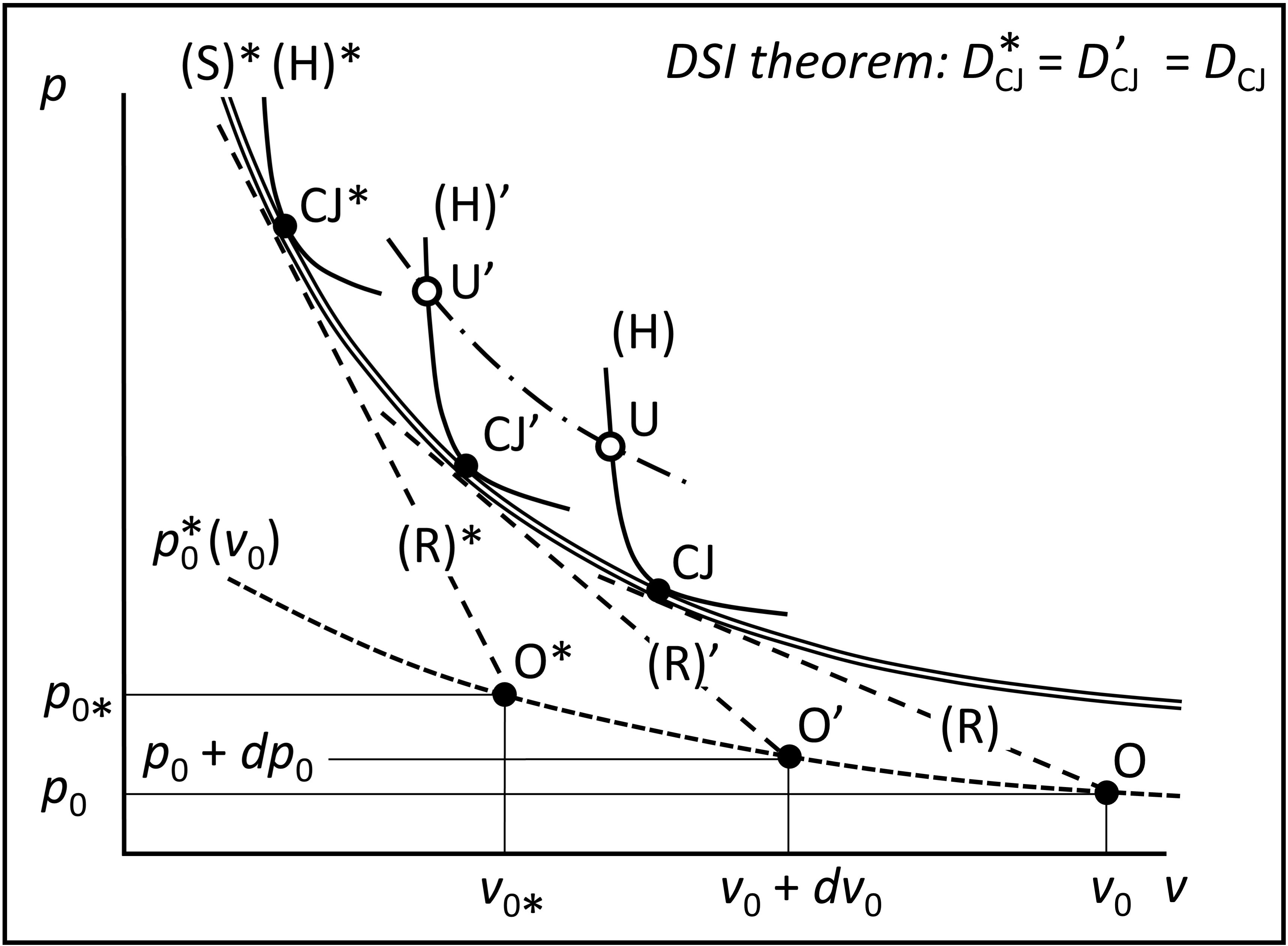
Figure 1: An equilibrium isentrope of detonation products (S)* can be the common envelope of equilibrium Hugoniot curves (H)*, (H)’ and (H) and Rayleigh-Michelson lines (R)*, (R)’ and (R) if their poles O*, O’ and O lie on a particular ${p}_{0}^{\ast}{\ (v}_{0}{)}$ line through a reference initial state O*${(p}_{0\ast}{,v}_{0\ast}{)}$ (the Hugoniot curvatures are accentuated). The slopes ${-(D}_{\text{CJ}}{\ /v}_{0}{)}^{2}$of these (R) lines increase with increasing initial volume $v_{0}$, but the DSI theorem ensures they have the same CJ velocity ${D}_{\text{CJ}}^{\ast}$. This determines the CJ*, CJ’ and CJ states, the ${p}_{0}^{\ast}{(v}_{0}{)}$ initial states, and the isentrope (S)*, given ${D}_{\text{CJ}}^{\ast}$ and the initial sound speeds and Gruneisen coefficients.

Efforts today focus less on the physical relevance of the CJ model than on the identification and the modelling of the processes in the reaction zone of detonation, namely chemical changes, losses, adiabatic or not, cellular instabilities in homogeneous explosives, the condensation of carbon or local heat exchanges between grains in heterogeneous explosives, nonlocal thermodynamics. Most of them can prevent reaching the CJ-equilibrium state. The CJ model is essentially an ideal thermodynamic limit useful for calibrating the equations of state of detonation products whether or not the reactive flow reaches chemical equilibrium.

Is the detonation regime identifiable from experimental detonation velocities and pressures? Models are generally rejected if they cannot represent the observations. However, the differences may be due to inaccurate measurements or nonphysical parameters, the assumptions may not be physically relevant to the experiments, and an agreement should not exclude fewer assumptions. Equations of state of detonation products are calibrated by fitting the calculated CJ properties to the experimental values, but no criteria ensure the latter are those of the CJ-equilibrium detonation. This study proposes they are not if they do not satisfy the supplemental properties.

To some degree, this work also extends the semi-empirical Inverse Method of Jones [2], Stanyukovich [3] and Manson [4]. The Inverse Method gives the CJ hydrodynamic variables from experimental values of $D_{\text{CJ}}$ and its derivatives with respect to two independent initial-state variables, such as $p_{0}$ and $T_{0}$ (Subsect. III-D, §2); this work shows that the only value of $D_{\text{CJ}}$ is sufficient.

Section II is a reminder on classical but necessary elements that also introduces the main notation, Section III sets out the DSI theorem and the supplemental CJ properties, Section IV is an analysis of their agreements or differences with calculations or measurements for gases and liquids, and Section V is a summary with some speculative conclusions.

II Reminders and notation

The CJ postulate is that the sonic and equilibrium constraints are satisfied at the same position in the flow. This is in fact more of an ideal mathematical limit than observable physical reality. The traditional introduction to this old issue is the Zel’dovich-von Neuman-Döring (ZND) detonation model, namely a leading shock supported by a subsonic laminar reaction zone [5]. In a self-sustained detonation, the interplay between flow dynamics and physicochemical processes is such that the sonic front of the rear expansion maintains a sufficient distance from the shock so that the chemical processes achieve enough progress. The main difficulty is that the ZND model uses the frozen sound speed, while the CJ model uses the equilibrium sound speed.

II.1 Where the Chapman-Jouguet model lies

Most explosive devices have finite transverse dimensions, so self-sustained detonations are nonideal, with diverging reaction zones that encompass a frozen sonic locus, hence curved leading shocks and lower velocities than the plane CJ one: the flow behind the sonic locus cannot sustain the shock. However, any reaction process cannot reach CJ equilibrium as the steady planar limit of a frozen-sonic curved ZND detonation [6]. Higgins [7] presented several examples of equilibrium-frozen issues and nonideal detonations.

At the sonic locus, the rates of reaction processes, possibly nonmonotonic, exothermic or endothermic [8, 9], have to offset those of losses, such as heat transfer, friction or transverse expansion of the reaction zone so that the flow derivatives can remain finite there. The dynamics of a self-sustained ZND detonation is thus described by an Eigen-constraint between the parameters of the reaction and loss rates [10] and those of the leading-shock, namely its normal velocity, acceleration and curvature [11, 12, 13, 14]. Achieving the CJ balance at least requires set-ups large enough so that losses are negligible and the detonation front is flat, and distances from the ignition position long enough so that the gradients of the expanding flow of products are small and the chemical equilibrium can shift continuously.

Reaction processes differ for gases and liquids. For gases, up to moderately large equivalence ratios (ER), the prevailing view is that the translation, rotation and vibration degrees of freedom re-equilibrate much faster than chemical kinetics. For liquids, molecular-bond breaking would make the deexcitation time of vibrations comparable to that of chemical relaxation [15]. Tarver [16] gave an introduction to the Non-Equilibrium ZND model. Local thermodynamic equilibrium would be reached before chemical transformation in such gases but perhaps not in the detonation products of liquids. For gases with very large ERs, several works, e.g. [17, 18, 19, 20], point out that the condensation of solid carbon decreases the detonation velocity with increasing ERs faster than predicted by calculations that model the detonation products as a homogeneous gas. Carbon condensation is inherent to detonation in many condensed explosives [21, 22, 23]. The DSI theorem is limited to detonation products described as a single-phase fluid at chemical equilibrium.

The main criticism of the ZND model for homogeneous explosives is the instability of their reaction zones. They are not laminar, and detonation fronts have a three-dimensional cellular structure. In gases, the flow advects unburnt pockets, and the experimental mean widths of detonation cells are 10 to 50 times greater than calculated characteristic thicknesses of steady planar ZND reaction zones [24, 25], even if defining such widths can be difficult. In liquids, instabilities have often been observed, but their relation to chemical kinetics and their similarities to those in gases are still being investigated [23, 26, 27, 28, 29]. The surface areas of the detonation front or the cross-section of the experimental device at least have to be large enough compared to those of the instabilities for the CJ properties can be representative averages.

The supplemental CJ properties in this work do not aim at indicating which of the CJ assumptions is not satisfied, namely sonic chemical equilibrium, single-phase fluid, or laminar flow. On this point, they provide a simple criterion for determining whether the CJ-equilibrium model can represent experimental and numerical data because they do not necessitate specifying the equation of state.

II.2 Thermodynamic and hydrodynamic relations

The two basic independent thermodynamic variables for single-phase inviscid fluids, inert or at chemical equilibrium, are temperature $T$ and pressure $p$. In hydrodynamics, the specific volume $v\left(T,p\right)$ is more convenient than $T$ because it appears explicitly in the balance equations. Specific enthalpy $h$ and entropy $s$ are the main state functions used in this work. Their differentials write

$$dh\left(s,p\right) =Tds+vdp,$$ (1)

$$dh\left(p,v\right) =\frac{G+1}{G}vdp+\frac{c^{2}}{G}\frac{dv}{v},$$ (2)

$$dh\left(T,p\right) =C_{p}dT+\left(1-\frac{T}{v}\left.\frac{\partial v}{\partial T}\right)_{p}\right)vdp,$$ (3)

$$Tds\left(p,v\right) =\frac{vdp}{G}+\frac{c^{2}}{G}\frac{dv}{v},$$ (4)

$$c^{2} =Gv\left.\frac{\partial h}{\partial v}\right)_{p}=-v^{2}\left.\frac{\partial p}{\partial v}\right)_{s},$$ (5)

$$G =\frac{v}{\left.\frac{\partial h}{\partial p}\right)_{v}-v}=-\frac{v}{T}\left.\frac{\partial T}{\partial v}\right)_{s},$$ (6)

where $G$ is the Gruneisen coefficient, $C_{p}$ is the heat capacity at constant pressure, and $c$ is the sound speed. In gases, the adiabatic exponent $\gamma$ conveniently defines $c$ by

$$c^{2}=\gamma pv,\quad\gamma=-\frac{v}{p}\left.\frac{\partial p}{\partial v}\right)_{s}.$$ (7)

In the $p$-$v$ plane, isentropes ($ds=0$) have negative slopes since $\gamma>0$. The fundamental derivative of hydrodynamics $\Gamma$ [30, 31, 32, 33] defines their convexity. Most fluids have uniformly convex isentropes, their slopes monotonically decrease with increasing volume ($\Gamma>0$),

$$\!\!\Gamma=\frac{1}{2}\frac{v^{3}}{c^{2}}\left.\frac{\partial^{2}p}{\partial v^{2}}\right)_{s}\!\!=\frac{-v}{2}\left.\frac{\partial^{2}p}{\partial v^{2}}\right)_{s}\!/\left.\frac{\partial p}{\partial v}\right)_{s}\!\!=1-\frac{v}{c}\left.\frac{\partial c}{\partial v}\right)_{s}.$$ (8)

The fresh (initial, subscript $0$) and the equilibrium (final, no subscript) states of a reactive medium have different chemical compositions, and thus different state functions and coefficients. Typically, $\gamma<\gamma_{0}$ and, if products are brought from a $\left(T,p\right)$ equilibrium state to the $\left(T_{0},p_{0}\right)$ initial state, $v\left(T_{0},p_{0}\right)>v_{0}=v_{0}\left(T_{0},p_{0}\right)$ and $h\left(T_{0},p_{0}\right)<h_{0}=h_{0}\left(T_{0},p_{0}\right)$. The difference of enthalpies $Q_{0}=h_{0}\left(T_{0},p_{0}\right)-h\left(T_{0},p_{0}\right)$ is the heat of reaction at constant pressure.

Conservation of mass, momentum and energy surface fluxes through hydrodynamic discontinuities is expressed by the Rankine-Hugoniot relations, which, along the normal to the discontinuity, write

$$\rho_{0}D =\rho\left(D-u\right),$$ (9)

$$p_{0}+\rho_{0}D^{2} =p+\rho\left(D-u\right)^{2},$$ (10)

$$h_{0}+\frac{1}{2}D^{2} =h+\frac{1}{2}\left(D-u\right)^{2},$$ (11)

where $\rho=1/v$ is the specific mass, and $u$ and $D$ are the material speed and the discontinuity velocity in a laboratory-fixed frame, with initial state at rest ($u_{0}=0$). These relations combined with an $h\left(p,v\right)$ equation of state are not a closed system since there are 4 equations for the 5 variables $v$, $p$, $h$, $u$ and $D$, given an initial state $\left(p_{0},v_{0}\right)$ and $h_{0}\left(p_{0},v_{0}\right)$, hence a one-variable solution, for example,

$$p,v,h,u,T,s,c,\gamma,\Gamma,G,\;...\equiv\eta\left(D;v_{0},p_{0}\right).$$ (12)

Its representation in the $p$-$v$ plane (Fig. 2) is an intersect of a Rayleigh-Michelson (R) line $p_{\text{R}}\left(v,D;v_{0},p_{0}\right)$ and the Hugoniot (H) curve $p_{\text{H}}\left(v;v_{0},p_{0}\right)$,

$$p_{\text{R}}: p =p_{0}+\left(\frac{D}{v_{0}}\right)^{2}\left(v_{0}-v\right),$$ (13)

$$p_{\text{H}}: h\left(p,v\right) =h_{0}\left(p_{0},v_{0}\right)+\frac{1}{2}\left(p-p_{0}\right)\left(v_{0}+v\right).$$ (14)

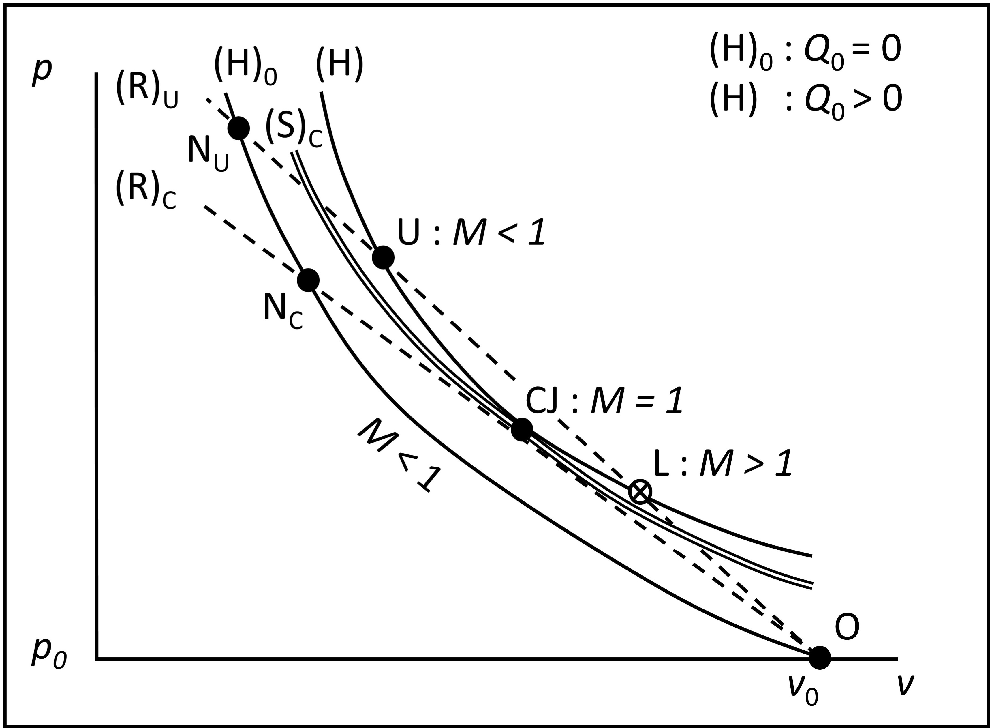
Figure 2: Unreacted (H)₀ and equilibrium (H) Hugoniot curves, and Rayleigh-Michelson lines (R)${}_{\text{U}}$ and (R)${}_{\text{C}}$ for discontinuity velocities greater than or equal to ${D}_{\text{CJ}}$. The physical intersects are points N, U and CJ ${(M\leqslant 1}$. The CJ isentrope (S)${}_{\text{C}}$ is positioned between the (R)${}_{\text{C}}$ line and the (H) curve.

A Hugoniot for a detonation ($Q_{0}>0$, $v\left(T_{0},p_{0}\right)>v_{0}$) lies above that for a shock ($Q_{0}=0$, $v\left(T_{0},p_{0}\right)=v_{0}$): most fluids have uniformly convex Hugoniots with 1 compressive intersect (N, $v/v_{0}<1$) if $Q_{0}=0$ regardless of $D$, and 2 (U and L) if $Q_{0}>0$ and $D$ is large enough. The observability of states on nonuniformly convex Hugoniots is an open debate on whether theoretical instability criteria are met in Nature, based on linear and nonlinear stability analyses of discontinuities [34, 35, 36, 37, 38]. At least physical admissibility (the discontinuity increases entropy, $s>s_{0}$) or equivalently mathematical determinacy (uniqueness and continuous dependency of (12) on the boundaries) have to be satisfied [39, 40, 41]. Denoting by $M_{0}$ and $M$ the discontinuity Mach numbers relative to the initial and the final states, this is expressed by the subsonic-supersonic evolution condition

$$u+c>D>c_{0}\ \Leftrightarrow\ \frac{D}{c_{0}}=M_{0}>1>M=\frac{D-u}{c}.$$ (15)

II.3 Chapman-Jouguet states and velocities,
and a remark

The tangency of a Rayleigh-Michelson line $p_{\text{R}}\left(v;D\right)$, an equilibrium Hugoniot $p_{\text{H}}\left(v\right)$ and an isentrope $p_{\text{S}}\left(v\right)$ defines CJ points and is equivalent to the sonic condition

$$M_{\text{CJ}}=\left(\frac{D-u}{c}\right)_{\text{CJ}}=1\text{ or }D_{\text{CJ}}=\left(u+c\right)_{\text{CJ}},$$ (16)

as shown by

$$\left.\frac{\partial p_{\text{R}}}{\partial v}\right)_{D,p_{0},v_{0}} =-\left(\frac{D}{v_{0}}\right)^{2}<0,$$ (17)

$$\left.\frac{\partial p_{\text{S}}}{\partial v}\right)_{s} =-\left(\frac{D}{v_{0}}\right)^{2}\times M^{-2}<0,$$ (18)

$$\left.\frac{\partial p_{\text{H}}}{\partial v}\right)_{p_{0},v_{0}} =-\left(\frac{D}{v_{0}}\right)^{2}\times\left(1+2\frac{M^{-2}-1}{F}\right),$$ (19)

$$F\left(G,v;v_{0}\right) =2-G\left(\frac{v_{0}}{v}-1\right).$$ (20)

There are 2 CJ points on uniformly convex Hugoniots (Fig. 3). The upper, compressive, one (CJc) is the CJ detonation, with velocity supersonic relative to the initial state ($v_{\text{CJ}}/v_{0}<1$, $p_{\text{CJ}}/p_{0}>1$, $D_{\text{CJc}}/c_{0}>1$). The lower, expansive, one (CJx) is the CJ deflagration, with velocity subsonic relative to the initial state ($v_{\text{CJ}}/v_{0}>1$, $p_{\text{CJ}}/p_{0}<1$, $D_{\text{CJx}}/c_{0}<1$).

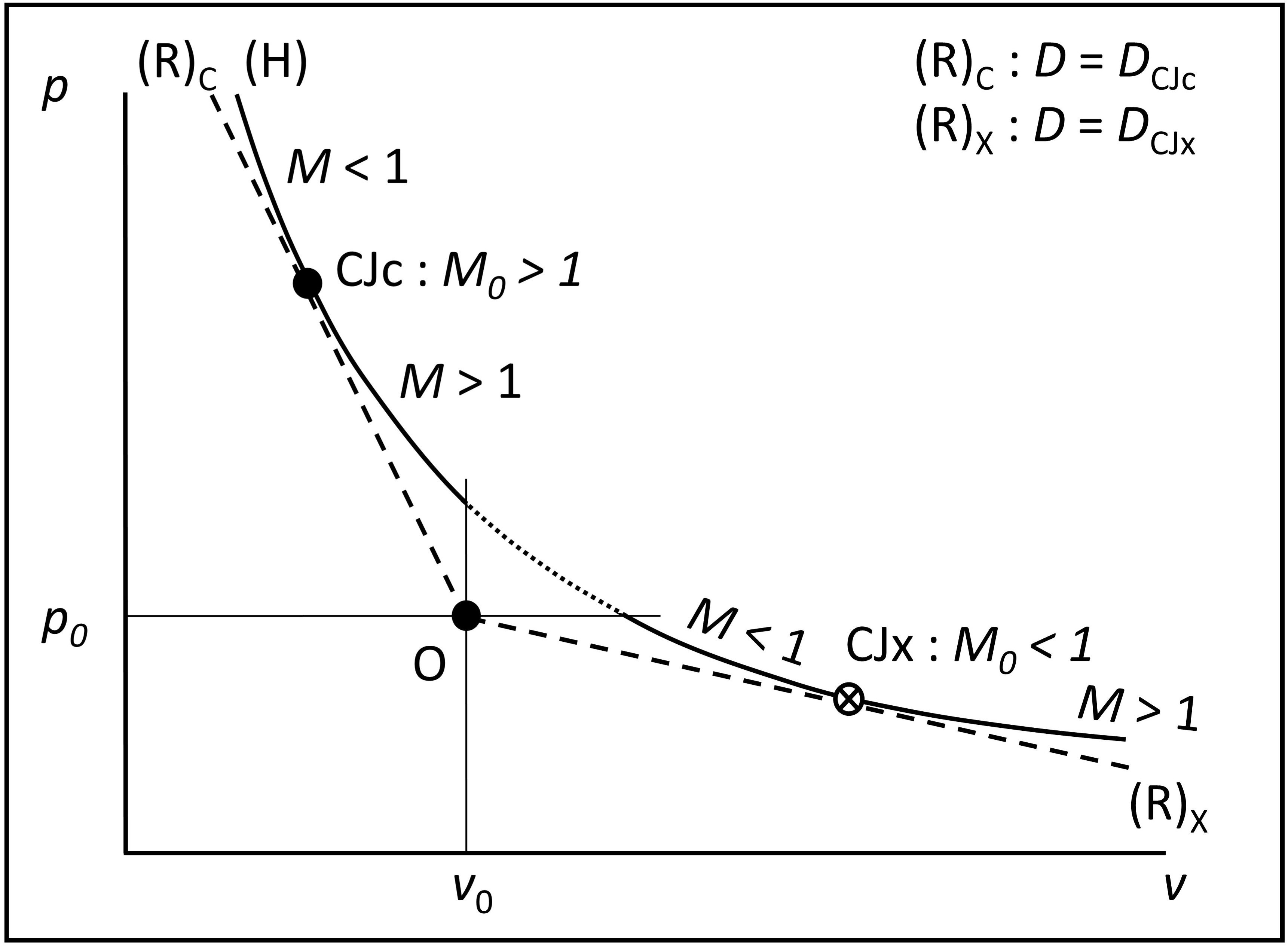
Figure 3: Detonation (upper) and deflagration (lower) Hugoniot arcs. The physical branch is above the compressive CJ point CJc.

The admissibility of the CJ detonation (App. B) requires $\Gamma_{\text{CJ}}>0$, so $F>0$ about and at a CJ point, the physical branch of an equilibrium Hugoniot arc is convex and above the CJ point as $M$ decreases from $1$ and $s$ increases with decreasing $v$, and $p_{\text{S}}\left(v\right)$ is positioned between $p_{\text{H}}\left(v\right)$ and $p_{\text{R}}\left(v\right)$ if $G>0$. The other properties useful here are $0\leqslant\left.\partial s_{\text{H}}/\partial D\right)_{p_{0},v_{0}}<\infty$ regardless of $M$, and, since $F_{\text{CJ}}\neq 0$, $\left.\partial s_{\text{H}}/\partial v\right)_{p_{0},v_{0}}^{\text{CJ}}=0$ and $\left.\partial D/\partial v\right)_{p_{0},v_{0}}^{\text{CJ}}=0$, as shown by

$$\frac{v_{0}T}{D^{2}}\left.\frac{\partial s_{\text{R}}}{\partial v}\right)_{D,p_{0},v_{0}} =\frac{v}{v_{0}}\frac{M^{-2}-1}{G},$$ (21)

$$\frac{v_{0}T}{D^{2}}\left.\frac{\partial s_{\text{H}}}{\partial v}\right)_{p_{0},v_{0}} =-\left(1-\frac{v}{v_{0}}\right)\frac{M^{-2}-1}{F},$$ (22)

$$\frac{T}{D}\left.\frac{\partial s_{\text{H}}}{\partial D}\right)_{p_{0},v_{0}} =\left(1-\frac{v}{v_{0}}\right)^{2}>0,$$ (23)

$$\frac{v_{0}}{D}\left.\frac{\partial D}{\partial v}\right)_{p_{0},v_{0}} =-\left(1-\frac{v}{v_{0}}\right)^{-1}\frac{M^{-2}-1}{F}.$$ (24)

The CJ condition (16) closes system (2), (9)-(11): the one-variable solution (12) and (16) give the CJ velocities $D_{\text{CJ}}$ and variables $\eta_{\text{CJ}}=\left(p,v,h,u,T,s,c,\gamma,\Gamma,G,\text{...}\right)_{\text{CJ}}$ as functions of the initial state,

$$D_{\text{CJ}}=D_{\text{CJ}}\left(v_{0},p_{0}\right),\quad\eta_{\text{CJ}}=\eta_{\text{CJ}}\left(v_{0},p_{0}\right).$$ (25)

The CJ detonation properties are calculated through thermochemical codes implementing physical equilibrium equations of state and thermodynamic properties at high pressures and temperatures. Simple $h\left(p,v\right)$ equations of state give explicit formulas (App. A).

The hydrodynamic variables $\left(p,v,u,c,h\right)$ at CJ points have a well-known two-variable representation as functions of $D_{\text{CJ}}$ and $\gamma_{\text{CJ}}$

$$\left(p,v,u,c,h\right)_{\text{CJ}}=y_{\text{CJ}}\left(D_{\text{CJ}},\gamma_{\text{CJ}};v_{0},p_{0}\right),$$ (26)

obtained by combining (7), the mass balance (9), the (R) relation (13) and the CJ condition (16),

$$\frac{v_{\text{CJ}}}{v_{0}} =\frac{c_{\text{CJ}}}{D_{\text{CJ}}}=\frac{\gamma_{\text{CJ}}}{\gamma_{\text{CJ}}+1}\left(1+\frac{p_{0}v_{0}}{D_{\text{CJ}}^{2}}\right),$$ (27)

$$\frac{v_{0}p_{\text{CJ}}}{D_{\text{CJ}}^{2}} =\frac{1+\frac{p_{0}v_{0}}{D_{\text{CJ}}^{2}}}{\gamma_{\text{CJ}}+1},\hskip 14.22636pt\frac{u_{\text{CJ}}}{D_{\text{CJ}}}=\frac{1-\gamma_{\text{CJ}}\frac{p_{0}v_{0}}{D_{\text{CJ}}^{2}}}{\gamma_{\text{CJ}}+1}.$$ (28)

The Hugoniot relation (14) then gives $h_{\text{CJ}}$.

The zero-variable representation (25) is obtained from a complete set that includes the energy balance and an explicit equation of state, hence the two-variable representation (26) since it does not use these two relations. The DSI theorem (Sect. III) supplements (26) with the energy balance, hence the primary consequence that the $y_{\text{CJ}}$’s above and $\gamma_{\text{CJ}}$ are explicit one-variable functions of $D_{\text{CJ}}$ (Subsect. III-D),

$$y_{\text{CJ}}=y_{\text{CJ}}\left(D_{\text{CJ}};v_{0},p_{0}\right),\;\gamma_{\text{CJ}}=\gamma_{\text{CJ}}\left(D_{\text{CJ}};v_{0},p_{0}\right).$$ (29)

Conversely, $D_{\text{CJ}}$ is a function of one CJ variable, for example, $D_{\text{CJ}}\left(\gamma_{\text{CJ}};v_{0},p_{0}\right)$. The NASA computer program CEA [42] for calculating chemical equilibria in ideal gases is used in subsection IV-A for investigating the theorem and generating CJ properties for comparison to the theoretical ones (29).

III The invariance theorem

Considering different initial states of the same homogeneous explosive, equivalent statements are:

1. the CJ detonation velocity $D_{\text{CJ}}$ and specific entropy $s_{\text{CJ}}$ are invariant under the same initial-state variation;

2. CJ detonations with the same $D_{\text{CJ}}$ have the same $s_{\text{CJ}}$, and conversely;

3. different initial states that produce the same $D_{\text{CJ}}$ determine different CJ states on the same isentrope;

4. an isentrope is the common envelope of Hugoniot curves and Rayleigh-Michelson lines of CJ detonations with the same velocity.

The CJ detonation state is a solution to the compatibility constraint on these initial variations. The subsections below detail the initial-variation problem, the Rankine-Hugoniot differentials, the theorem demonstration and its geometrical interpretation (Fig. 1), and the supplemental CJ properties.

III.1 The initial-variation problem

The simplest flow behind a plane discontinuity of velocity $D$ on a constant initial state $\left(v_{0},p_{0}\right)$ is that supported by a piston of constant speed $u_{\text{p}}$. The flow is constant-state regardless of $u_{\text{p}}$ behind a shock with the same initial and final composition, but only if $u_{\text{p}}$ is greater than the CJ speed $u_{\text{CJ}}$ in (28) behind a detonation with final burnt state at chemical equilibrium. Its speed relative to the discontinuity is subsonic ($D-u<c$). This defines the constant-velocity overdriven detonation. The final-state variables $\eta=\left(p,v,h,T,s,c,\gamma,\Gamma,G,\text{ ...}\right)$, with $u=u_{\text{p}}$, are one-variable functions (Subsect. II-B), such as $D\left(u;v_{0},p_{0}\right)$ and $\eta\left(u;v_{0},p_{0}\right)$, or $\eta\left(D;v_{0},p_{0}\right)$ (12), for example, (118).

If $u_{\text{p}}$ is smaller than $u_{\text{CJ}}$, the flow is expanding and supersonic relative to the detonation front ($D-u>c$) but sonic just at the front. The CJ-equilibrium condition is indeed a consequence of the Taylor-Zel’dovich-Döring (TZD) simple-wave solution $\eta\left(x/t\right)$ to the homentropic flow (uniform $s$) behind this constant-velocity plane front: $u+c=x/t\Rightarrow\left(u+c\right)_{\text{CJ}}=x_{\text{CJ}}\left(t\right)/t\equiv D_{\text{CJ}}$, with $t$ the time and $x$ the position in the flow [43, 44, 10]. In contrast to the overdriven detonation, no perturbation in the flow can reach the front: $x<x_{\text{CJ}}\Rightarrow x/t=u+c<x_{\text{CJ}}/t=\left(u+c\right)_{\text{CJ}}=D_{\text{CJ}}$. This defines the CJ self-sustained detonation (Subsect. II-C, App. B). The CJ velocity and state are then the functions $D_{\text{CJ}}\left(v_{0},p_{0}\right)$ and $\eta_{\text{CJ}}\left(v_{0},p_{0}\right)$ (25) of the only initial state, for example, (27), (28) and (114) .

If $u_{\text{p}}$ is exactly set to $u_{\text{CJ}}$, the flow is both constant-state and sonic regardless of $x$ and $t$: $u+c=\left(u+c\right)_{\text{CJ}}=x_{\text{CJ}}\left(t\right)/t=D_{\text{CJ}}$. The velocity $D$ is still equal to $D_{\text{CJ}}\left(v_{0},p_{0}\right)$, which, therefore, is also the smallest value reachable in a series of experiments, each carried out with constant values of $u_{p}$ greater than, but closer and closer to $u_{\text{CJ}}\left(v_{0},p_{0}\right)$ from one experiment to the other. This is also the limiting TZD flow for infinite run distances of a CJ detonation from ignition at a fixed wall ($u_{p}=0$): the slopes of the $\eta\left(x/t\right)$ profiles tend to zero with increasing $t$ at fixed position $x$.

An overdriven detonation can thus have the same velocity $D$ with different initial states $\left(v_{0},p_{0}\right)$ if $u_{\text{p}}$ is set to the value greater than $u_{\text{CJ}}\left(v_{0},p_{0}\right)$ that ensures $D\left(u_{\text{p}};v_{0},p_{0}\right)=$ const. There is no reason then why one of the final-state variables should also be invariant. For the CJ detonation, the same initial states turn out to ensure that both $D_{\text{CJ}}$ and $s_{\text{CJ}}$ are constant. The invariance of one ensures the other.

Specific entropy $s$ enters the problem only through the differentials of $h\left(s,p\right)$ (1) and $s\left(p,v\right)$ (4), so this initial-variation problem has to be formulated as $ds=0$ and $dD=0$, which entails differentiating the Rankine-Hugoniot relations (9)-(11).

III.2 Rankine-Hugoniot differentials

Using the dimensionless hydrodynamic variable

$$z=\;1-\frac{v}{v_{0}}=\frac{v_{0}\left(p-p_{0}\right)}{D^{2}}=\frac{u}{D},$$ (30)

the differentials of the Rayleigh-Michelson line (13), the Hugoniot relation (14) and the $h\left(p,v\right)$ equation of state (2) form the $3\times 3$ nonhomogeneous linear system for $dv$, $dp$ and $dh$

$$\frac{v_{0}dp}{D^{2}}+\frac{dv}{v_{0}}=2z\frac{dD}{D}-\left(2z-1\right)\frac{dv_{0}}{v_{0}}+\frac{v_{0}dp_{0}}{D^{2}},$$ (31)

$$2\frac{dh}{D^{2}}-\left(2-z\right)\frac{v_{0}dp}{D^{2}}-z\frac{dv}{v_{0}}=\;...$$

$$\quad\quad\quad...\;z\frac{dv_{0}}{v_{0}}-\left(2-z\right)\frac{v_{0}dp_{0}}{D^{2}}+2\frac{dh_{0}}{D^{2}},$$ (32)

$$\frac{G}{1-z}\frac{dh}{D^{2}}-\left(G+1\right)\frac{v_{0}dp}{D^{2}}-M^{-2}\frac{dv}{v_{0}}=0,$$ (33)

which thus are linear combinations of $dD$, $dv_{0}$, $dp_{0}$ and $dh_{0}\left(p_{0},v_{0}\right)$. For example, with the notation $F\left(G,z\right)$ (20),

$$\left(M^{-2}-1\right)\frac{v_{0}dp}{D^{2}}=z\left(F+2\left(M^{-2}-1\right)\right)\frac{dD}{D}\;...\\ ...\;-\left(1-F\left(1-z\right)+\left(M^{-2}-1\right)\left(2z-1\right)\right)\frac{dv_{0}}{v_{0}}\;...\quad\\ ...\;+\left(\frac{1+\left(1-F\right)\left(1-z\right)}{z}+M^{-2}-1\right)\frac{v_{0}dp_{0}}{D^{2}}\;...\quad\\ ...\;-\frac{2-F}{z}\frac{dh_{0}}{D^{2}},$$ (34)

$$\left(M^{-2}-1\right)\frac{dv}{v_{0}}=-zF\frac{dD}{D}\;...\\ ...\;+\left(1-F\left(1-z\right)\right)\frac{dv_{0}}{v_{0}}-\frac{2-z-F\left(1-z\right)}{z}\frac{v_{0}dp_{0}}{D^{2}}\;...\\ ...\;+\frac{2-F}{z}\frac{dh_{0}}{D^{2}}.$$ (35)

The differential $ds$ of the specific entropy,

$$\frac{Tds}{D^{2}}=\;...\\ ...\;z^{2}\frac{dD}{D}+\left(1-z\right)z\frac{dv_{0}}{v_{0}}-\left(1-z\right)\frac{v_{0}dp_{0}}{D^{2}}+\frac{dh_{0}}{D^{2}},$$ (36)

is obtained by using $dh\left(s,p\right)$ (1) instead of $dh\left(p,v\right)$ (33) in (32). The state functions $c$ and $G$ are not involved in $dh\left(s,p\right)$, so neither are $M$ and $F$ in $ds$ (36).

The determinant of system (31)-(33) is $M^{-2}-1$, and the right-hand sides of (35) and (34) have to be set to zero for CJ discontinuities ($M=1$) so that $dv$ and $dp$ can be finite, hence the Eigen-constraints for the differentials $dD_{\text{CJ}}$ and $ds_{\text{CJ}}$ of the CJ velocity and entropy

$$\frac{dD_{\text{CJ}}}{D_{\text{CJ}}} =\frac{2-F_{\text{CJ}}}{F_{\text{CJ}}z_{\text{CJ}}^{2}}\frac{dh_{0}}{D_{\text{CJ}}^{2}}+\frac{1-F_{\text{CJ}}\left(1-z_{\text{CJ}}\right)}{F_{\text{CJ}}z_{\text{CJ}}}\frac{dv_{0}}{v_{0}}\;...$$

$$...-\;\frac{2-z_{\text{CJ}}-F_{\text{CJ}}\left(1-z_{\text{CJ}}\right)}{F_{\text{CJ}}z_{\text{CJ}}^{2}}\frac{v_{0}dp_{0}}{D_{\text{CJ}}^{2}},$$ (37)

$$\frac{T_{\text{CJ}}ds_{\text{CJ}}}{D_{\text{CJ}}^{2}} =\frac{2}{F_{\text{CJ}}}\frac{dh_{0}}{D_{\text{CJ}}^{2}}+\frac{z_{\text{CJ}}}{F_{\text{CJ}}}\frac{dv_{0}}{v_{0}}-\frac{2-z_{\text{CJ}}}{F_{\text{CJ}}}\frac{v_{0}dp_{0}}{D_{\text{CJ}}^{2}}.$$ (38)

They can be directly obtained from (31) and (32) by using $dh\left(s,p\right)$ (1) and $ds\left(p,v\right)$ (4), the CJ condition $M=1$ in the form $c/v=D/v_{0}$ (9) and then eliminating the combination $v_{0}dp_{\text{CJ}}/D_{\text{CJ}}^{2}+dv_{\text{CJ}}/v_{0}$ [4, 45]. The intermediate differentials (35) and (36) are necessary to demonstrate the DSI theorem. The CJ differentials (37) and (38) show that $F_{\text{CJ}}\neq 0$ (20) is also the continuity condition that small initial variations produce small variations of $D_{\text{CJ}}$ and $s_{\text{CJ}}$ (Subsect. II-B, App. B). In the acoustic limit ($D\rightarrow c_{0}$, $v/v_{0}\rightarrow 1$, $z\rightarrow 0$, $F\rightarrow 2$), (36) and (38) coherently reduce to $dh_{0}\left(s_{0},p_{0}\right)$.

Replacing $dh_{0}$ by $dh_{0}\left(p_{0},v_{0}\right)$ (2) written as

$$\frac{dh_{0}}{D^{2}}=\frac{G_{0}+1}{G_{0}}\frac{v_{0}dp_{0}}{D^{2}}+\frac{M_{0}^{-2}}{G_{0}}\frac{dv_{0}}{v_{0}},$$ (39)

introducing

$$\varepsilon =M^{-2}-1,$$ (40)

$$A =z+\frac{2M_{0}^{-2}}{G_{0}},\!\!\! B =z+\frac{2}{G_{0}},$$ (41)

$$a =z\left(1-z\right)+\frac{M_{0}^{-2}}{G_{0}},\!\!\! b =z+\frac{1}{G_{0}},$$ (42)

and denoting by

$$v_{s}=v\left(s;v_{0},p_{0}\right)\quad\text{and}\quad v_{D}=v\left(D;v_{0},p_{0}\right)$$ (43)

the specific volume expressed in the sets of independent variables $\left(s,v_{0},p_{0}\right)$ and $\left(D,v_{0},p_{0}\right)$, the differentials of $dv$ (35) and $ds$ (36) condense to

$$\varepsilon z\frac{dv_{s}}{v_{0}} =A\frac{dv_{0}}{v_{0}}+B\frac{v_{0}dp_{0}}{D^{2}}-F\frac{Tds}{D^{2}},$$ (44)

$$\varepsilon z\frac{dv_{D}}{v_{0}} =\left(A-aF\right)\frac{dv_{0}}{v_{0}}+\left(B-bF\right)\frac{v_{0}dp_{0}}{D^{2}}-z^{2}F\frac{dD}{D},$$ (45)

$$\frac{Tds}{D^{2}} =z^{2}\frac{dD}{D}+a\frac{dv_{0}}{v_{0}}+b\frac{v_{0}dp_{0}}{D^{2}},$$ (46)

and $ds_{\text{CJ}}$ and $dD_{\text{CJ}}$ to

$$z_{\text{CJ}}^{2}F_{\text{CJ}}\frac{dD_{\text{CJ}}}{D_{\text{CJ}}} =\left(A_{\text{CJ}}-a_{\text{CJ}}F_{\text{CJ}}\right)\frac{dv_{0}}{v_{0}}\;...$$

$$...+\left(B_{\text{CJ}}-b_{\text{CJ}}F_{\text{CJ}}\right)\frac{v_{0}dp_{0}}{D^{2}},$$ (47)

$$F_{\text{CJ}}\frac{T_{\text{CJ}}ds_{\text{CJ}}}{D_{\text{CJ}}^{2}} =A_{\text{CJ}}\frac{dv_{0}}{v_{0}}+B_{\text{CJ}}\frac{v_{0}dp_{0}}{D_{\text{CJ}}^{2}}.$$ (48)

III.3 Demonstration and interpretation

The premise is that the variations of the initial state lead to finite variations of the final state. In particular, the slopes of admissible constant-$s$ and constant-$D$ arcs are finite since the physical values of $D_{\text{CJ}}$ and its variations are (Subsect. III-D).

The differentials of $v\left(s;v_{0},p_{0}\right)$ and $v\left(D;v_{0},p_{0}\right)$ write

$$\!\!dv_{s} =\left.\frac{\partial v_{s}}{\partial v_{0}}\right)_{p_{0},s}\!\!\!\!\!dv_{0}+\left.\frac{\partial v_{s}}{\partial p_{0}}\right)_{v_{0},s}\!\!\!\!\!dp_{0}+\left.\frac{\partial v_{s}}{\partial s}\right)_{p_{0},v_{0}}\!\!\!ds,$$ (49)

$$\!\!dv_{D} =\left.\frac{\partial v_{D}}{\partial v_{0}}\right)_{p_{0},D}\!\!\!\!\!dv_{0}+\left.\frac{\partial v_{D}}{\partial p_{0}}\right)_{v_{0},D}\!\!\!\!\!dp_{0}+\left.\frac{\partial v_{D}}{\partial D}\right)_{p_{0},v_{0}}\!\!\!\!\!dD,$$ (50)

where, from (44) and (45),

$$\varepsilon z\left.\frac{\partial v_{s}}{\partial v_{0}}\right)_{p_{0},s}=A,\quad\varepsilon z\left.\frac{\partial v_{D}}{\partial v_{0}}\right)_{p_{0},D}=A-aF,$$ (51)

$$\varepsilon z\left.\frac{\partial v_{s}}{\partial p_{0}}\right)_{v_{0},s}=B,\quad\varepsilon z\left.\frac{\partial v_{D}}{\partial p_{0}}\right)_{v_{0},D}=B-bF,$$ (52)

and

$$\varepsilon z\frac{D^{2}}{v_{0}T}\left.\frac{\partial v_{s}}{\partial s}\right)_{p_{0},v_{0}}=\varepsilon z^{-1}\frac{D}{v_{0}}\left.\frac{\partial v_{D}}{\partial D}\right)_{p_{0},v_{0}}=-F.$$ (53)

It is convenient to distribute the initial states $p_{0}$ and $v_{0}$ on arbitrary polar curves $p_{0}^{\ast}\left(v_{0}\right)$ through a reference point $v_{0\ast},p_{0\ast}=p_{0}^{\ast}\left(v_{0\ast}\right)$ (O^∗, Fig. 1). Their slopes $dp_{0}^{\ast}/dv_{0}$ determine the changes of the initial and the final properties. Initial states varying on a curve $p_{0}^{\ast}\left(v_{0}\right)$ generate a $\left(p\text{-}v\right)$ arc of final states between a point U on a Hugoniot H with pole O$\left(v_{0},p_{0}=p_{0}^{\ast}\left(v_{0}\right)\right)$ and a point U’ on another Hugoniot H’ with pole O’$\left(v_{0}+dv_{0},p_{0}+dp_{0}^{\ast}\right)$. Final states varying at constant initial state lie on the same Hugoniot as (22)-(24) or (53) express. The total derivatives of $v_{D}=v\left(D;v_{0},p_{0}\right)$ along an isentrope ($s=$ const.) and of $v_{s}=v\left(s;v_{0},p_{0}\right)$ along an iso-velocity arc ($D=$ const.) thus write

$$\left.\frac{dv_{D}}{dv_{0}}\right|_{s} =\left.\frac{\partial v_{D}}{\partial v_{0}}\right)_{s}+\left.\frac{\partial v_{D}}{\partial D}\right)_{p_{0},v_{0}}\left.\frac{dD}{dv_{0}}\right|_{s},$$ (54)

$$\left.\frac{dv_{s}}{dv_{0}}\right|_{D} =\left.\frac{\partial v_{s}}{\partial v_{0}}\right)_{D}+\left.\frac{\partial v_{s}}{\partial s}\right)_{p_{0},v_{0}}\left.\frac{ds}{dv_{0}}\right|_{D},$$ (55)

where

$$\left.\frac{\partial v_{D}}{\partial v_{0}}\right)_{s}=\left.\frac{\partial v_{D}}{\partial v_{0}}\right)_{p_{0},D}+\left.\frac{\partial v_{D}}{\partial p_{0}}\right)_{v_{0},D}\left.\frac{dp_{0}^{\ast}}{dv_{0}}\right|_{s}=\;...$$

$$...\; \left.\frac{\partial v_{s}}{\partial v_{0}}\right)_{D}=\left.\frac{\partial v_{s}}{\partial v_{0}}\right)_{p_{0},s}+\left.\frac{\partial v_{s}}{\partial p_{0}}\right)_{v_{0},s}\left.\frac{dp_{0}^{\ast}}{dv_{0}}\right|_{D}.$$ (56)

The derivatives $\left.d./dv_{0}\right|_{s}$ are the variations for which a piston achieves a constant $s$ (Subsect. III-A); $\left.d./dv_{0}\right|_{D}$ are those for constant $D$. The derivatives $dp_{0}^{\ast}/dv_{0}$ in (56) for constant $s$ or $D$ are not unique.

The derivatives of $D$ and $s$ in (54) and (55) are obtained from (53), and differential (46) links their sum to the difference of the derivatives of $p_{0}^{\ast}$,

$$\frac{v_{0}}{D}\left.\frac{dD}{dv_{0}}\right|_{s} =\varepsilon\left(\left.\frac{\partial v_{D}}{\partial v_{0}}\right)_{s}-\left.\frac{dv_{D}}{dv_{0}}\right|_{s}\right)/zF,$$ (57)

$$\frac{v_{0}T}{D^{2}}\left.\frac{ds}{dv_{0}}\right|_{D} =\varepsilon\left(\left.\frac{\partial v_{s}}{\partial v_{0}}\right)_{D}-\left.\frac{dv_{s}}{dv_{0}}\right|_{D}\right)z/F,$$ (58)

$$z^{2}\frac{v_{0}}{D}\left.\frac{dD}{dv_{0}}\right|_{s} +\frac{v_{0}T}{D^{2}}\left.\frac{ds}{dv_{0}}\right|_{D}=\;...$$

$$...\;b\left(\left.\frac{dp_{0}^{\ast}}{dv_{0}}\right|_{D}-\left.\frac{dp_{0}^{\ast}}{dv_{0}}\right|_{s}\right)\left(\frac{v_{0}}{D}\right)^{2}.$$ (59)

The boundedness of the derivatives of $v$ with respect to the initial-state variations thus implies that, in the sonic limit $\varepsilon=0$ ($M=1,z\neq 0$, Subsect. III-A),

$$\left.\frac{dD}{dv_{0}}\right|_{s}^{\left(M=1\right)}=0,\quad\left.\frac{ds}{dv_{0}}\right|_{D}^{\left(M=1\right)}=0,$$ (60)

that is, from (59), the DSI theorem

$$\left(ds\right)^{\left(M=1\right)}\equiv ds_{\text{CJ}}=0\Leftrightarrow\left(dD\right)^{\left(M=1\right)}\equiv dD_{\text{CJ}}=0,$$ (61)

expressing the invariance of $s_{\text{CJ}}$ and $D_{\text{CJ}}$ for the same initial variation $dp_{0}^{\ast}$. The determinant of the system (47)-(48) must be zero so that $dp_{0}\neq 0$ and $dv_{0}\neq 0$ if $dD_{\text{CJ}}=0$ and $ds_{\text{CJ}}=0$, so

$$\!\!\!-\left(\frac{v_{0}}{D}\right)^{2}\left.\frac{dp_{0}^{\ast}}{dv_{0}}\right|_{\text{DSI}}\!\!\!=\frac{A_{\text{CJ}}}{B_{\text{CJ}}}=\frac{\left(A_{\text{CJ}}-a_{\text{CJ}}F_{\text{CJ}}\right)}{\left(B_{\text{CJ}}-b_{\text{CJ}}F_{\text{CJ}}\right)}=\frac{a_{\text{CJ}}}{b_{\text{CJ}}},$$ (62)

hence, with (41) and (42), the constraint on the CJ state

$$G_{0}z_{\text{CJ}}^{2}+2z_{\text{CJ}}-\left(1-M_{0\text{CJ}}^{-2}\right)=0.$$ (63)

An interpretation in the $p$-$v$ plane (Fig. 1) considers the Hugoniot curves $p_{\text{H}}\left(v;p_{0},v_{0}\right)$ (14) as a one-parameter family $y_{\text{H}}^{\ast}\left(p,v;v_{0}\right)=0$ with parameter $v_{0}$ if their poles $\left(p_{0},v_{0}\right)$ are distributed on $p_{0}^{\ast}\left(v_{0}\right)$,

$$y_{\text{H}}^{\ast}\left(p,v;v_{0}\right)=\;...$$

$$...\;-h\left(p,v\right)+h_{0}\left(p_{0}^{\ast},v_{0}\right)+\frac{1}{2}\left(p-p_{0}^{\ast}\right)\left(v_{0}+v\right).$$ (64)

This family has an envelope if $p_{0}^{\ast}\left(v_{0}\right)$ satisfies the condition obtained by setting to zero the partial derivative of $y_{\text{H}}^{\ast}\left(p,v;v_{0}\right)$ with respect to $v_{0}$

$$\!\!\!\!\!\!\!\!\left.\frac{\partial y_{\text{H}}^{\ast}}{\partial v_{0}}\right)_{p,v}\!=0\Leftrightarrow-\left(\frac{v_{0}}{D}\right)^{2}\frac{dp_{0}^{\ast}}{dv_{0}}=\frac{z+\frac{2M_{0}^{-2}}{G_{0}}}{z+\frac{2}{G_{0}}}=\frac{A}{B}.$$ (65)

The CJ-entropy differential (48) shows that this envelope is an isentrope if it is made up of sonic points.

Similarly, the Rayleigh-Michelson lines (R) $p_{\text{R}}\left(v,D;p_{0},v_{0}\right)$ (14) form a two-parameter family $y_{\text{R}}^{\ast}\left(p,v;D,v_{0}\right)=0$, with parameters $v_{0}$ and $D$, if their poles $\left(p_{0},v_{0}\right)$ are distributed on $p_{0}^{\ast}\left(v_{0}\right)$,

$$y_{\text{R}}^{\ast}\left(p,v;D,v_{0}\right)=-p+p_{0}^{\ast}+\left(\frac{D}{v_{0}}\right)^{2}\left(v_{0}-v\right),$$ (66)

which reduces to a one-parameter ($v_{0}$) sub-family if $D$ is varied with $v_{0}$ and $p_{0}$. Setting to zero the partial derivative of $y_{\text{R}}^{\ast}\left(p,v;D\left(v_{0}\text{,}p_{0}^{\ast}\left(v_{0}\right)\right),v_{0}\right)$ with respect to $v_{0}$ thus gives the condition for the R lines to have an envelope

$$\!\!\!\!\!\!\!\!\left.\frac{\partial y_{\text{H}}^{\ast}}{\partial v_{0}}\right)_{p,v}\!=0\Leftrightarrow-\left(\frac{v_{0}}{D}\right)^{2}\frac{dp_{0}^{\ast}}{dv_{0}}=1-2z+2z\frac{v_{0}}{D}\frac{dD}{dv_{0}}.$$ (67)

which is an isentrope if it is made up of sonic points. This can be observed from

$$\frac{G}{1-z}\frac{Tds_{\text{R}}}{D^{2}}=\frac{v_{0}dp_{0}}{D^{2}}+\left(1-2z\right)\frac{dv_{0}}{v_{0}}\;...$$

$$...\;+2z\frac{dD}{D}+\left(M^{-2}-1\right)\frac{dv}{v_{0}},$$ (68)

obtained by combining the differentials of the R relation (31) and the $s\left(p,v\right)$ equation of state (4). If $D=D_{\text{CJ}}$, (68) and the DSI condition that $dD_{\text{CJ}}=0$ along an isentrope lead to

$$-\left(\frac{v_{0}}{D_{\text{CJ}}}\right)^{2}\frac{dp_{0}^{\ast}}{dv_{0}}=1-2z_{\text{CJ}}.$$ (69)

Identifying the envelope conditions (65) and (69) returns the constraint (63) on the CJ state. The identities (56)-(58) show that an isentrope and a constant-velocity arc have a second-order contact at CJ points ($z\neq 0$).

An isentrope is thus the common envelope (Fig. 1) of families of equilibrium Hugoniots and Rayleigh-Michelson lines with initial states such that CJ detonations have the same velocity. The relation with Davis’implementation of the Inverse Method for condensed explosives [46] is discussed in subsection III-D, §2 and 3.

III.4 Supplemental Chapman-Jouguet properties

D.1. CJ state and isentrope. The CJ detonation state is the compressive solution ($z_{\text{CJ}}>0$) of equation (63) ensuring nonzero variations $dp_{0}$ and $dv_{0}$ for the joint invariance of $D_{\text{CJ}}$ and $s_{\text{CJ}}$. Using (27), (28) and (30), this one-variable ($D_{\text{CJ}}$) representation (29) writes

$$v_{\text{CJ}}\left(D_{\text{CJ}};v_{0},p_{0}\right)=v_{0}\frac{1+G_{0}-\sqrt{1+G_{0}\left(1-M_{0\text{CJ}}^{-2}\right)}}{G_{0}},$$ (70)

$$p_{\text{CJ}}\left(D_{\text{CJ}};v_{0},p_{0}\right)=p_{0}+\frac{D_{\text{CJ}}^{2}}{v_{0}}\frac{\sqrt{1+G_{0}\left(1-M_{0\text{CJ}}^{-2}\right)}-1}{G_{0}},\quad$$ (71)

$$\gamma_{\text{CJ}}\left(D_{\text{CJ}};v_{0},p_{0}\right)=...$$

$$\;\;\;\;...\;\frac{1+G_{0}-\sqrt{1+G_{0}\left(1-M_{0\text{CJ}}^{-2}\right)}}{G_{0}\frac{p_{0}v_{0}}{c_{0}^{2}}M_{0\text{CJ}}^{-2}-1+\sqrt{1+G_{0}\left(1-M_{0\text{CJ}}^{-2}\right)}}.$$ (72)

Conversely, $D_{\text{CJ}}$ is a function of one CJ variable, for example, the dimensionless pressure jump $\pi_{\text{CJ}}=v_{0}\left(p_{\text{CJ}}-p_{0}\right)/c_{0}^{2}$ from (63) or (71)) or the adiabatic exponent $\gamma_{\text{CJ}}$ from (72). Hence,

$$\left(\frac{D_{\text{CJ}}}{c_{0}}\right)^{2}=\pi_{\text{CJ}}\left(1+\frac{1}{2\pi_{\text{CJ}}}\right)\left(1+\sqrt{1+\frac{G_{0}}{\left(1+\frac{1}{2\pi_{\text{CJ}}}\right)^{2}}}\right),$$ (73)

$$\left(\frac{D_{\text{CJ}}}{c_{0}}\right)^{2}=\frac{1}{2}\frac{\left(\gamma_{\text{CJ}}+1\right)^{2}}{\gamma_{\text{CJ}}^{2}-1-G_{0}}\times\left\{1-2\frac{1+\frac{G_{0}}{\gamma_{\text{CJ}}+1}}{\gamma_{\text{CJ}}+1}\frac{\gamma_{\text{CJ}}}{\widetilde{\gamma}_{0}}\right.\;...$$

$$\quad\quad\quad...\;+\left.\sqrt{1-4\frac{1+\frac{G_{0}-\left(1+G_{0}\right)\frac{\gamma_{\text{CJ}}}{\widetilde{\gamma}_{0}}}{\gamma_{\text{CJ}}+1}}{\gamma_{\text{CJ}}+1}\frac{\gamma_{\text{CJ}}}{\widetilde{\gamma}_{0}}}\right\},$$ (74)

where $\widetilde{\gamma}_{0}=c_{0}^{2}/p_{0}v_{0}$ and should not be confused with $\gamma_{0}$, except for gases (Subsect. II-A). Relation (74) shows a large sensitivity of $D_{\text{CJ}}$ to $\gamma_{\text{CJ}}$, as is more evident in the gas example below from (77). The identity

$$G_{0}=\frac{\alpha_{0}c_{0}^{2}}{C_{p_{0}}},\;\alpha_{0}=\frac{1}{v_{0}}\left.\frac{\partial v_{0}}{\partial T_{0}}\right)_{p_{0}},$$ (75)

indicates that the necessary initial data are $c_{0}$, $C_{p_{0}}$, and $v_{0}$ measured as a function of $T_{0}$ at constant $p_{0}$ so the coefficient of thermal expansion $\alpha_{0}$ can be determined.

For ideal gases, $c$, $C_{p}$, $\alpha$ and $\gamma$ are functions of $T=pv\left(W/R\right)$ only, $G=$ $\gamma-1$, $v=RT/pW$, $\alpha=1/T$. Thus, for initially ideal gases,

$$\gamma_{\text{CJ}}\left(D_{\text{CJ}},p_{0},T_{0}\right)=\sqrt{\frac{\gamma_{0}}{1-\frac{\gamma_{0}-1}{\gamma_{0}}M_{0\text{CJ}}^{-2}}}\;,$$ (76)

$$D_{\text{CJ}}^{2}\left(\gamma_{\text{CJ}},p_{0},T_{0}\right)=\frac{1-\gamma_{0}^{-1}}{1-\frac{\gamma_{0}}{\gamma_{\text{CJ}}^{2}}}\times c_{0}^{2}\;,$$ (77)

$$\frac{D_{\text{CJ}}^{2}\left(p_{\text{CJ}},p_{0},T_{0}\right)}{v_{0}p_{\text{CJ}}}=\left(1-\left(1-\frac{\gamma_{0}}{2}\right)\frac{p_{0}}{p_{\text{CJ}}}\right)\times\;...$$

$$\quad\quad\quad...\;\left\{1+\sqrt{1+\frac{\left(\gamma_{0}-1\right)\left(1-\frac{p_{0}}{p_{\text{CJ}}}\right)^{2}}{\left(1-\left(1-\frac{\gamma_{0}}{2}\right)\frac{p_{0}}{p_{\text{CJ}}}\right)^{2}}}\right\}.$$ (78)

The strong-shock limits ($M_{0\text{CJ}}^{-2}\ll 1$ or $p_{0}/p_{\text{CJ}}\ll 1$) of $\gamma_{\text{CJ}}$ and $D_{\text{CJ}}^{2}$ are $\sqrt{\gamma_{0}}$ and $\left(1+\sqrt{\gamma_{0}}\right)v_{0}p_{\text{CJ}}$, respectively (their acoustic limits are $\gamma_{0}$ and $c_{0}^{2}$). The typical values $\gamma_{0}=1.3$, $c_{0}=330$ m/s and $D_{\text{CJ}}=2000$ m/s give $\gamma_{\text{CJ}}=1.144$, $\sqrt{\gamma_{0}}=1.140$ and relative error $100\times\left(\gamma_{\text{CJ}}/\sqrt{\gamma_{0}}-1\right)=0.316$ %. Relations (76)-(78) apply only to initially ideal gases, but products can be nonideal if $p_{0}$ is large enough.

The polar curve $p_{0}^{\ast}\left(v_{0}\right)$ that generates the invariance of $D_{\text{CJ}}$ and $s_{\text{CJ}}$ is solution to the ordinary differential equation formed by substituting (70) for $v$ in (65) or (69). The initial condition is the reference initial state $\left(p_{0\ast},v_{0\ast}\right)$ with known CJ velocity $D_{\text{CJ}}^{\ast}$. Substitution for $p_{0}$ in $v_{\text{CJ}}$ (70) and $p_{\text{R}}$ (13) gives

$$v_{\text{CJ}}^{\ast}\left(v_{0}\right) =v_{\text{CJ}}\left(v_{0},p_{0}^{\ast}\left(v_{0}\right),D_{\text{CJ}}^{\ast}\right),$$ (79)

$$p_{\text{CJ}}^{\ast}\left(v_{0}\right) =p_{0}^{\ast}\left(v_{0}\right)+\frac{D_{\text{CJ}}^{\ast 2}}{v_{0}}\left(1-\frac{v_{\text{CJ}}^{\ast}\left(v_{0}\right)}{v_{0}}\right).$$ (80)

The isentrope $p_{\text{S}}^{\ast}\left(v\right)$ is generated by eliminating $v_{0}$ between $v_{\text{CJ}}^{\ast}\left(v_{0}\right)$ and $p_{\text{CJ}}^{\ast}\left(v_{0}\right)$, that is, by varying $v_{0}$ and representing $p_{\text{CJ}}^{\ast}\left(v_{0}\right)$ as a function of $v_{\text{CJ}}^{\ast}\left(v_{0}\right)$. Thus, $v_{0}$ can parametrize an isentrope of detonation products. This, however, necessitates determining $C_{p_{0}}$, $c_{0}$ and $v_{0}$ in a sufficiently large $\left(p_{0},T_{0}\right)$ domain.

The DSI theorem holds if the isentropes have finite slopes so the derivatives $\left.dz/dv_{0}\right|_{s}$ and $\left.dz/dv_{0}\right|_{D}$ can be finite and nonzero at sonic points (Subsect. III-C). This condition is obtained by differentiating $c\left(s,v\right)$ (5) and the mass balance (9-a) written as $v=v_{0}M\left(c/D\right)$,

$$\frac{dv}{v} =\frac{dv_{0}}{v_{0}}+\frac{dc}{c}+\frac{dM}{M}-\frac{dD}{D},$$ (81)

$$dc =\left.\frac{\partial c}{\partial s}\right)_{v}ds+\left.\frac{\partial c}{\partial v}\right)_{s}dv,$$ (82)

hence, restricting variations to an isentrope,

$$\Gamma\frac{v_{0}}{v}\left.\frac{dv}{dv_{0}}\right|_{s}=1-\frac{v_{0}}{D}\left.\frac{dD}{dv_{0}}\right|_{s}+\frac{v_{0}}{M}\left.\frac{dM}{dv_{0}}\right|_{s},$$ (83)

with $\Gamma$ the fundamental derivative of hydrodynamics (8). The CJ condition $M=$ const. $=1$, the DSI property $\left.dD/dv_{0}\right|_{s}^{\left(M=1\right)}=0$ (60), (7), (1) and (9), then give

$$\left.\frac{dv}{dv_{0}}\right|_{s}^{\left(M=1\right)}=-\left(\frac{v_{0}}{D_{\text{CJ}}}\right)^{2}\left.\frac{dp}{dv_{0}}\right|_{s}^{\left(M=1\right)}=\Gamma_{\text{CJ}}^{-1}\frac{v_{\text{CJ}}}{v_{0}},$$ (84)

$$\frac{v_{0}}{D_{\text{CJ}}^{2}}\left.\frac{dh}{dv_{0}}\right|_{s}^{\left(M=1\right)}=-\Gamma_{\text{CJ}}^{-1}\left(\frac{v_{\text{CJ}}}{v_{0}}\right)^{2},$$ (85)

$$\frac{v_{0}}{D_{\text{CJ}}}\left.\frac{du}{dv_{0}}\right|_{s}^{\left(M=1\right)}=\left(1-\Gamma_{\text{CJ}}^{-1}\right)\frac{v_{\text{CJ}}}{v_{0}}.$$ (86)

The derivatives of $v$, $p$ and $h$ at constant $s$ (or $D$ from (61)) are thus finite and nonzero at a CJ point except if $\Gamma_{\text{CJ}}=0$ and $\Gamma_{\text{CJ}}\rightarrow\infty$ respectively (the derivative of $u$ is zero for $\Gamma_{\text{CJ}}=1$). In contrast, their derivatives $\left.\partial./\partial D\right)_{v_{0},p_{0}}^{\left(M=1\right)}$ at constant initial state – along the same Hugoniot – are infinite, that is, $\left.\partial D/\partial.\right)_{v_{0},p_{0}}^{\left(M=1\right)}=0$ (24), (45). In the perfect-gas example (App. A), taking the partial derivative of $v\left(D;v_{0},p_{0}\right)$ (118) with respect to $D$ moves the square-root term to the denominator, so lim${}_{D\rightarrow D_{\text{CJ}}}\left.\partial v/\partial D\right)_{p_{0},v_{0}}=-\infty$, whereas its derivative with respect to $v_{0}$ at constant $D$, with $p_{0}=p_{0}^{\ast}\left(v_{0}\right)$, shows that lim${}_{D\rightarrow D_{\text{CJ}}}\left.dv/dv_{0}\right|_{D}\$is finite if $\left.dD/dv_{0}\right|_{s}=0$. An expression for $\Gamma_{\text{CJ}}=\left.d\ln v/dv_{0}\right|_{s}^{\left(M=1\right)}$ (84) that combines the partial derivatives of $\gamma_{0}$ and $G_{0}$ can be obtained by differentiating the DSI constraint (63) with respect to $v_{0}$ at constant $D_{\text{CJ}}$.

The ratio $dD_{\text{CJ}}/ds_{\text{CJ}}$ is obtained by eliminating $dp_{0}/dv_{0}$ between (47) and (48). The nonhomogeneous term is zero from (63), hence

$$\frac{D_{\text{CJ}}dD_{\text{CJ}}}{T_{\text{CJ}}ds_{\text{CJ}}}=z_{\text{CJ}}^{-2}\left(1-F_{\text{CJ}}\frac{1+G_{0}z_{\text{CJ}}}{2+G_{0}z_{\text{CJ}}}\right).$$ (87)

The partial derivatives of $D_{\text{CJ}}\left(v_{0},p_{0}\right)$ and $D_{\text{CJ}}\left(T_{0},p_{0}\right)$ are not independent since there are initial-state variations for which $D_{\text{CJ}}$ is constant. This follows from the triple product rule,

$$\left.\frac{\partial D_{\text{CJ}}}{\partial y_{0}}\right)_{p_{0}}=-\left.\frac{\partial p_{0}}{\partial y_{0}}\right)_{D_{\text{CJ}}}\left.\frac{\partial D_{\text{CJ}}}{\partial p_{0}}\right)_{y_{0}},$$ (88)

where $y_{0}$ denotes either $v_{0}$ or $T_{0}$. Hence, with $\left.\partial p_{0}/\partial v_{0}\right)_{D_{\text{CJ}}}$ given by (65) or (69),

$$\frac{v_{0}}{D_{\text{CJ}}} \left.\frac{\partial D_{\text{CJ}}}{\partial v_{0}}\right)_{p_{0}}=\frac{D_{\text{CJ}}}{v_{0}}\left.\frac{\partial D_{\text{CJ}}}{\partial p_{0}}\right)_{v_{0}}\times\left(1-2z_{\text{CJ}}\right),$$ (89)

$$\frac{D_{\text{CJ}}}{v_{0}} \left.\frac{\partial D_{\text{CJ}}}{\partial p_{0}}\right)_{T_{0}}=\frac{T_{0}}{D_{\text{CJ}}}\left.\frac{\partial D_{\text{CJ}}}{\partial T_{0}}\right)_{p_{0}}\times\;...$$

$$...\;\frac{1-\left(1+\alpha_{0}T_{0}G_{0}\right)\left(1-2z_{\text{CJ}}\right)M_{0\text{CJ}}^{2}}{\left(1-2z_{\text{CJ}}\right)\alpha_{0}T_{0}}.$$ (90)

The latter is obtained from the former and the identities

$$\frac{T_{0}}{D_{\text{CJ}}}\left.\frac{\partial D_{\text{CJ}}}{\partial T_{0}}\right)_{p_{0}}=\alpha_{0}T_{0}\frac{v_{0}}{D_{\text{CJ}}}\left.\frac{\partial D_{\text{CJ}}}{\partial v_{0}}\right)_{p_{0}},$$ (91)

$$\frac{D_{\text{CJ}}}{v_{0}}\left.\frac{\partial D_{\text{CJ}}}{\partial p_{0}}\right)_{T_{0}}=\frac{v_{0}}{D_{\text{CJ}}}\left.\frac{\partial D_{\text{CJ}}}{\partial p_{0}}\right)_{v_{0}}\;...$$

$$\;\;\;\;\;...\;-M_{0}^{2}\left(1+\alpha_{0}T_{0}G_{0}\right)\frac{v_{0}}{D_{\text{CJ}}}\left.\frac{\partial D_{\text{CJ}}}{\partial v_{0}}\right)_{p_{0}}.$$ (92)

The variations of $D_{\text{CJ}}$ with respect to $T_{0}$ at constant $p_{0}$ thus determine those with respect to $p_{0}$ at constant $T_{0}$, and conversely. The constraints (88)-(92) also apply to $s_{\text{CJ}}$ since $\left.\partial p_{0}/\partial y_{0}\right)_{D_{\text{CJ}}}=\left.\partial p_{0}/\partial y_{0}\right)_{s_{\text{CJ}}}$.

D.2. The Inverse Method (IM). This reminder is useful to discuss below the DSI theorem, and its application to liquid explosives in subsection IV-B. The IM gives the CJ state from $D_{\text{CJ}}$ and its derivatives with respect to two independent initial-state variables (Sect. I). Manson [4] and Wood and Fickett [45] examined several IM options depending on the pair of variables; the two used in this work derive from (37).

The first one uses the pair $\left(T_{0},p_{0}\right)$. Measurements of $D_{\text{CJ}}\left(T_{0},p_{0}\right)$ give its partial derivatives, substituting (39) for $dh_{0}\left(p_{0},v_{0}\right)$ reduces (37) to the differential (47) of $D_{\text{CJ}}\left(v_{0},p_{0}\right)$, and eliminating $F_{\text{CJ}}$ (or $G_{\text{CJ}}$) (20) between its coefficients then gives the CJ state as the solution $z_{\text{CJ}}<1$ of

$$G_{0}Lz_{\text{CJ}}^{2}+2Kz_{\text{CJ}}-\left(1-M_{0\text{CJ}}^{-2}\right)=0,$$ (93)

where $L$ and $K$ for $D_{\text{CJ}}\left(v_{0},p_{0}\right)$ and $D_{\text{CJ}}\left(T_{0},p_{0}\right)$ are

$$L =1+\frac{D_{\text{CJ}}}{v_{0}}\left.\frac{\partial D_{\text{CJ}}}{\partial p_{0}}\right)_{v_{0}}-\frac{v_{0}}{D_{\text{CJ}}}\left.\frac{\partial D_{\text{CJ}}}{\partial v_{0}}\right)_{p_{0}}$$

$$=\ 1+\frac{D_{\text{CJ}}}{v_{0}}\left.\frac{\partial D_{\text{CJ}}}{\partial p_{0}}\right)_{T_{0}}\;...$$

$$...\;+\frac{1-M_{0\text{CJ}}^{-2}+\alpha_{0}T_{0}G_{0}}{\alpha_{0}T_{0}M_{0\text{CJ}}^{-2}}\frac{T_{0}}{D_{\text{CJ}}}\left.\frac{\partial D_{\text{CJ}}}{\partial T_{0}}\right)_{p_{0}},$$ (94)

$$K =1+M_{0\text{CJ}}^{-2}\frac{D_{\text{CJ}}}{v_{0}}\left.\frac{\partial D_{\text{CJ}}}{\partial p_{0}}\right)_{v_{0}}-\frac{v_{0}}{D_{\text{CJ}}}\left.\frac{\partial D_{\text{CJ}}}{\partial v_{0}}\right)_{p_{0}}$$

$$= 1+M_{0\text{CJ}}^{-2}\frac{D_{\text{CJ}}}{v_{0}}\left.\frac{\partial D_{\text{CJ}}}{\partial p_{0}}\right)_{T_{0}}+\frac{G_{0}T_{0}}{D_{\text{CJ}}}\left.\frac{\partial D_{\text{CJ}}}{\partial T_{0}}\right)_{p_{0}},$$ (95)

through $dv_{0}\left(T_{0},p_{0}\right)$ and $dh_{0}\left(T_{0},p_{0}\right)$ (75). The IM relation (93) also writes

$$G_{0}z_{\text{CJ}}^{2}+2z_{\text{CJ}}-\left(1-M_{0\text{CJ}}^{-2}\right)-L^{-1}\left(1-M_{0\text{CJ}}^{-2}\right)\times\;...$$

$$...\;\left(\left(1-2z_{\text{CJ}}\right)\left.\frac{\partial D_{\text{CJ}}}{\partial p_{0}}\right)_{v_{0}}-\left.\frac{\partial D_{\text{CJ}}}{\partial v_{0}}\right)_{p_{0}}\right)=0,$$ (96)

which reduces to the DSI relation (63) by demanding that the partial derivatives of $D_{\text{CJ}}$ meet their DSI compatibility relation (89). It should be emphasized that any assumption on the derivatives of $D_{\text{CJ}}$ such that $L$ and $K$ are each equal to $1$ also reduces (93) to (63). Such assumptions are nonphysical because they select the acoustic-limit solution $M_{0\text{CJ}}=1$ – $D_{\text{CJ}}=c_{0}$, $z_{\text{CJ}}=0$ – of the DSI and IM relations (63) and (93), which the expressions of $L$ and $K$ above show. Manson [47] had noted the strong-shock limit $\sqrt{\gamma_{0}}$ of $\gamma_{\text{CJ}}$ for the ideal gas (76) by neglecting the dimensionless partial derivatives $\left.\partial\ln D_{\text{CJ}}/\partial\ln p_{0}\right)_{T_{0}}$ and $\left.\partial\ln D_{\text{CJ}}/\partial\ln T_{0}\right)_{p_{0}}$. This contradicts the distinguished limit required by the large values of $M_{0\text{CJ}}^{2}$ in their coefficients in (94): the determinants of the $2\times 2$ linear systems for the partial derivatives of $D_{\text{CJ}}\left(v_{0},p_{0}\right)$ and $D_{\text{CJ}}\left(T_{0},p_{0}\right)$, with $L-1$ and $K-1$ as nonhomogeneous terms, are proportional to $M_{0\text{CJ}}^{-2}-1$, which therefore must be zero regardless of the magnitudes of these derivatives, even very small.

The second option uses the pair $\left(v_{0},h_{0}\right)$ at constant $p_{0}$. Their variations can be obtained from a set of isometric mixtures [48], that is, with the same atomic composition, and hence the same equilibrium equation of state, for any value of a composition parameter, denoted below by $w_{0}$ after [45]. Typically, $w_{0}$ is the total volume- or mass-fraction of all compounds added to the reference composition. The initial and CJ properties of the reference explosive are then defined by $w_{0}=0$. Measurements of $v_{0}\left(T_{0},w_{0}\right)$, $h_{0}\left(T_{0},w_{0}\right)$ and $D_{\text{CJ}}\left(T_{0},w_{0}\right)$ at constant $p_{0}$ give their partial derivatives, setting $dp_{0}=0$ in (37) gives the differential of $D_{\text{CJ}}\left(v_{0},h_{0}\right)$, and eliminating $F_{\text{CJ}}$ between its coefficients then gives the CJ state as the solution $z_{\text{CJ}}<1$ of

$$Lz_{\text{CJ}}^{2}+2Kz_{\text{CJ}}-1=0,$$ (97)

where $L$ and $K$ for $D_{\text{CJ}}\left(v_{0},h_{0}\right)$ and $D_{\text{CJ}}\left(T_{0},w_{0}\right)$ are

$$L =\ D_{\text{CJ}}\left.\frac{\partial D_{\text{CJ}}}{\partial h_{0}}\right)_{v_{0},p_{0}}$$

$$=\;\frac{\frac{\omega_{0}T_{0}}{D_{\text{CJ}}}\left.\frac{\partial D_{\text{CJ}}}{\partial T_{0}}\right)_{w_{0},p_{0}}-\frac{\alpha_{0}T_{0}}{D_{\text{CJ}}}\left.\frac{\partial D_{\text{CJ}}}{\partial w_{0}}\right)_{T_{0},p_{0}}}{\omega_{0}\frac{C_{p_{0}}T_{0}}{D_{\text{CJ}}^{2}}-\alpha_{0}T_{0}\Omega_{0}},$$ (98)

$$K =\ 1-\frac{v_{0}}{D_{\text{CJ}}}\left.\frac{\partial D_{\text{CJ}}}{\partial v_{0}}\right)_{h_{0},p_{0}}$$

$$=1+\frac{\frac{\Omega_{0}D_{\text{CJ}}}{T_{0}}\left.\frac{\partial D_{\text{CJ}}}{\partial T_{0}}\right)_{w_{0},p_{0}}-\frac{C_{p_{0}}T_{0}}{D_{\text{CJ}}^{3}}\left.\frac{\partial D_{\text{CJ}}}{\partial w_{0}}\right)_{T_{0},p_{0}}}{\omega_{0}\frac{C_{p_{0}}T_{0}}{D_{\text{CJ}}^{2}}-\alpha_{0}T_{0}\Omega_{0}},$$ (99)

through the identities

$$\!\!\!\frac{dv_{0}}{v_{0}}=\alpha_{0}T_{0}\frac{dT_{0}}{T_{0}}+\omega_{0}dw_{0},\quad\;\omega_{0}=\frac{1}{v_{0}}\left.\frac{\partial v_{0}}{\partial w_{0}}\right)_{T_{0},p_{0}},$$ (100)

$$\!\!\!\frac{dh_{0}}{D^{2}}=\frac{C_{p_{0}}T_{0}}{D^{2}}\frac{dT_{0}}{T_{0}}+\Omega_{0}dw_{0},\ \Omega_{0}=\frac{1}{D^{2}}\left.\frac{\partial h_{0}}{\partial w_{0}}\right)_{T_{0},p_{0}}.$$ (101)

This option is more convenient than the first because it does not necessitate $c_{0}$ and generating sufficiently large variations of $p_{0}$ may be uneasy.

The main drawback of the IM is its limited accuracy because the partial derivatives of $D_{\text{CJ}}$ are measured independently of each other and cumulate their experimental uncertainties (Subsect. IV-B). The CJ state given by the DSI theorem requires only the value of $D_{\text{CJ}}$.

D.3. Remarks. The envelope conditions (Subsect. III-C) on $D$ and $h_{0}$ for the Rayleigh-Michelson (R) lines (13) and Hugoniot (H) curves (14) if $v_{0}$ and $h_{0}$ are independent at constant $p_{0}$ write, from (67) and (64),

$$\frac{v_{0}}{D}\frac{dD}{dv_{0}} =\;\frac{1}{2}\frac{1-2\frac{v}{v_{0}}}{1-\frac{v}{v_{0}}}=1-\left(2\frac{v_{0}\left(p-p_{0}\right)}{D^{2}}\right)^{-1},$$ (102)

$$\frac{v_{0}}{D^{2}}\frac{dh_{0}}{dv_{0}} =-\frac{1}{2}\left(1-\frac{v}{v_{0}}\right)=-\frac{1}{2}\frac{v_{0}\left(p-p_{0}\right)}{D^{2}},$$ (103)

respectively. From (68) and (102), a sonic envelope to the R lines is an isentrope, which combined with (36) indeed returns the envelope condition (103) for the H curves. The constraint $ds_{\text{CJ}}=0$ can be satisfied here, but not its DSI equivalence $dD_{\text{CJ}}=0$ because otherwise, from (102), $v_{\text{CJ}}/v_{0}=1/2$, that is, $\gamma_{\text{CJ}}=1$. The DSI theorem $ds_{\text{CJ}}=0\Leftrightarrow dD_{\text{CJ}}=0$ is physically valid only if $p_{0}$ is varied, even if $p_{0}/p$ or $v_{0}p_{0}/D^{2}$ are negligible, and for initial and final states described by two-variable equations of state $T\left(p,v\right)$.

Davis [46] implemented the IM for condensed explosives ($p_{0}/p\approx 10^{-5}$) with the specific energy $e_{0}$ and mass $\rho_{0}=1/v_{0}$ as independent initial-state variables, and negligible constant $p_{0}$. He built $D_{\text{CJ}}\left(e_{0},\rho_{0}\right)$ from Kamlet’s method, and calculated the poles $e_{0}^{\ast}\left(\rho_{0}\right)$ of Hugoniots with the same isentropic envelope, this isentrope and the CJ state. His relations (14) and (31) are equivalent to (102) and (103), respectively, because $e_{0}=h_{0}$ if $p_{0}$ is neglected. Nagayama and Kubota [49] derived an envelope constraint for the R lines from linear laws $D_{\text{CJ}}\left(\rho_{0}\right)$ with negligible dependency on $e_{0}$. Their relations (13) and (14) are equivalent to (102), that is, $z_{\text{CJ}}=1/2K$ from (97) and (98).

The differentials of the Rankine-Hugoniot relations and the equations of state form a $2\times 2$ homogeneous linear system for $dp_{0}$ and $dv_{0}$ – with $dh_{0}$ subject to (39) – for any invariant pair of final-state variables. Only the invariance of $D_{\text{CJ}}$ and $s_{\text{CJ}}$ produces nonzero and physical $dp_{0}$ and $dv_{0}$, that is, a non-trivially null determinant (63). Thus, no nonzero $dp_{0}$ and $dv_{0}$ permit a focal point in the $p$ - $v$ plane – $dp_{\text{CJ}}=0$ - $dv_{\text{CJ}}=0$ – because then $dh_{\text{CJ}}=0$ since $h=h\left(p,v\right)$, and $dD_{\text{CJ}}=0$ from (31), which represents the R line through $\left(p_{0},v_{0}\right)$.

Equilibrium compositions in homogeneous media are functions of $T$ and $p$, so the differentiations above implicitly take their variations into account with those of a $T\left(p,v\right)$ equation of state (Subsect. III-B). Further, there is no reason for different initial states to generate the same frozen final composition.

IV Application to
gaseous or liquid explosives

For gaseous explosives (Subsect. IV-A), the DSI theorem and some supplemental CJ properties were analysed through chemical equilibrium calculations. Only ideal detonation products were considered to avoid the uncertainties induced by equations of state calibrated from experiments that may not have achieved the strict CJ equilibrium, such as those of condensed explosives (Sect. I). The calculations were done with the NASA computer program CEA [42]. For liquid explosives (Subsect. IV-B), the analysis compares and discusses the theoretical CJ pressures from (71) and values from experiments and the Inverse Method (Subsect. III-D, §2).

IV.1 Gaseous explosives with ideal final states

Tables I show numerical values of $s_{\text{CJ}}$ and $D_{\text{CJ}}$ for the four stoichiometric mixtures $CH_{4}+2$ $O_{2}$, $C_{3}H_{8}+5$ $O_{2}$, $CH_{4}+2$ Air and $H_{2}+0.5$ Air. Five ($T_{0},p_{0}$) pairs with $T_{0}$ evenly spaced between $200$ and $400$ K were used to represent a largest physical range; the third – $T_{0}=298.15$ K, $p_{0}=1$ bar – was chosen as the reference initial state $\left(v_{0\ast},p_{0\ast}\right)$ (subscript $\ast$, Subsect. III-C). The values of $p_{0}$ were determined by dichotomy for each $T_{0}$ so all entropies have the reference value $s_{\text{CJ}}^{\ast}$. The results were analysed based on the mean velocities $\bar{D}_{\text{CJ}}$, the relative deviations $\Delta D_{\text{CJ}}/\bar{D}_{\text{CJ}}$ and their absolute means $m_{D_{\text{CJ}}}$ in percent, and the corrected standard deviations $\sigma_{D_{\text{CJ}}}$,

$$\bar{D}_{\text{CJ}}=\frac{1}{I}\sum_{i=1}^{I=5}D_{\text{CJ}i}\;,\ \left(\frac{\Delta D_{\text{CJ}}}{\bar{D}_{\text{CJ}}}\right)_{i}=100\times\frac{D_{\text{CJ}i}-\bar{D}_{\text{CJ}}}{\bar{D}_{\text{CJ}}},$$ (104)

$$\\ m_{D_{\text{CJ}}}=\frac{1}{I}\sum_{i=1}^{I=5}\left|\frac{\Delta D_{\text{CJ}}}{\bar{D}_{\text{CJ}}}\right|_{i}\;,\ \sigma_{D_{\text{CJ}}}=\sqrt{\sum_{i=1}^{I=5}\frac{\left(D_{\text{CJ}i}-\bar{D}_{\text{CJ}}\right)^{2}}{I-1}}.$$ (105)

All $m_{D_{\text{CJ}}}$’s and $\sigma_{D_{\text{CJ}}}$’s are very small. In particular, all $D_{\text{CJ}}$’s are close to their mean values $\bar{D}_{\text{CJ}}$ to $\mathcal{O}\left(0.1\right)$ % at most. The agreement is practically exact for $C_{3}H_{8}+5$ $O_{2}$. An iterative minimization of both $\Delta D_{\text{CJ}}/\bar{D}_{\text{CJ}}$ and $\Delta s_{\text{CJ}}/\bar{s}_{\text{CJ}}$ would probably return values of $p_{0}\left(T_{0}\right)$, $\bar{D}_{\text{CJ}}$ and $\bar{s}_{\text{CJ}}$ that even better satisfy the theorem and eliminate the slight decreasing trend of $D_{\text{CJ}}$ with increasing $T_{0}$ at constant $s_{\text{CJ}}^{\ast}$ observed here. The $p_{0}\left(T_{0}\right)$ values and the results in table I can be seen as zeroth-order iterates, so the $\left(v_{0}\left(T_{0}\right),p_{0}\right)$ pairs well approximate the polar curve $p_{0}^{\ast}\left(v_{0}\right)$ through $\left(v_{0\ast},p_{0\ast}\right)$ (Subsect. III-C). It is easy, albeit tedious, to check that another reference than $T_{0}^{\ast}=298.15$ K and $p_{0}^{\ast}=1$ bar returns values of $m_{D_{\text{CJ}}}$ and $\sigma_{D_{\text{CJ}}}$ similarly small.

Table 1: Joint invariances of the CJ entropy $s_{\text{CJ}}$ and velocity $D_{\text{CJ}}$ of 4 mixtures: mean value $\bar{D}_{\text{CJ}}$, relative deviation $\Delta D_{\text{CJ}}/\bar{D}_{\text{CJ}}$, mean relative deviation $m_{D_{\text{CJ}}}$, corrected standard deviation $\sigma_{D_{\text{CJ}}}$.

$CH_{4}+2\;O_{2}$		$m_{D_{\text{CJ}}}=\,0.08\text{ \%}$
$\bar{D}_{\text{CJ}}=\,2389.7\text{ m/s}$		$\sigma_{D_{\text{CJ}}}\;=\,2.47\text{ m/s}$
$T_{0}$	$p_{0}$	$s_{\text{CJ}}$	$D_{\text{CJ}}$	$\frac{\Delta D_{\text{CJ}}}{\bar{D}_{\text{CJ}}}$
(K)	(bar)	(kJ/kg/K)	(m/s)	(%)
$200.00$	$0.6284$	$id.$	$2392.9$	$0.13$
$250.00$	$0.8118$	$id.$	$2391.2$	$0.06$
$298.15^{\ast}$	$1.0000^{\ast}$	$12.6653^{\mathbf{\ast}}$	$2389.6$	$\sim 0.00$
$350.00$	$1.2165$	$id.$	$2388.0$	$-0.07$
$400.00$	$1.4410$	$id.$	$2386.7$	$-0.12$

$C_{3}H_{8}+5\;O_{2}$		$m_{D_{\text{CJ}}}=\,0.012\text{ \%}$
$\bar{D}_{\text{CJ}}=\,2356.7\text{ m/s}$		$\sigma_{D_{\text{CJ}}}\;=\,0.41\text{ m/s}$
$T_{0}$	$p_{0}$	$s_{\text{CJ}}$	$D_{\text{CJ}}$	$\frac{\Delta D_{\text{CJ}}}{\bar{D}_{\text{CJ}}}$
(K)	(bar)	(kJ/kg/K)	(m/s)	(%)
$200.00$	$0.6304$	$id.$	$2357.3$	$0.03$
$250.00$	$0.8127$	$id.$	$2356.7$	$\sim 0.00$
$298.15^{\mathbf{\ast}}$	$1.0000^{\mathbf{\ast}}$	$11.9293^{\mathbf{\ast}}$	$2356.3$	$-0.01_{5}$
$350.00$	$1.2165$	$id.$	$2356.3$	$-0.01_{5}$
$400.00$	$1.4419$	$id.$	$2356.7$	$\sim 0.00$

$CH_{4}+2\;\text{ Air}$		$m_{D_{\text{CJ}}}=\,0.05\text{ \%}$
$\bar{D}_{\text{CJ}}=\,1799.9\text{ m/s}$		$\sigma_{D_{\text{CJ}}}\;=\,1.23\text{ m/s}$
$T_{0}$	$p_{0}$	$s_{\text{CJ}}$	$D_{\text{CJ}}$	$\frac{\Delta D_{\text{CJ}}}{\bar{D}_{\text{CJ}}}$
(K)	(bar)	(kJ/kg/K)	(m/s)	(%)
$200.00$	$0.6044$	$id.$	$1801.4$	$0.08$
$250.00$	$0.7968$	$id.$	$1800.7$	$0.05$
$298.15^{\mathbf{\ast}}$	$1.0000^{\ast}$	$9.4218^{\ast}$	$1799.9$	$\sim 0.00$
$350.00$	$1.2401$	$id.$	$1799.1$	$-0.04$
$400.00$	$1.4949$	$id.$	$1798.3$	$-0.09$

$H_{2}+0.5\text{ Air}$		$m_{D_{\text{CJ}}}=\,0.1\text{ \%}$
$\bar{D}_{\text{CJ}}=\,1964.7\text{ m/s}$		$\sigma_{D_{\text{CJ}}}\;=\,2.55\text{ m/s}$
$T_{0}$	$p_{0}$	$s_{\text{CJ}}$	$D_{\text{CJ}}$	$\frac{\Delta D_{\text{CJ}}}{\bar{D}_{\text{CJ}}}$
(K)	(bar)	(kJ/kg/K)	(m/s)	(%)
$200.00$	$0.6004$	$id.$	$1967.9$	$0.16$
$250.00$	$0.7941$	$id.$	$1966.4$	$0.08$
$298.15^{\mathbf{\ast}}$	$1.0000^{\mathbf{\ast}}$	$10.5927^{\mathbf{\ast}}$	$1964.8$	$\sim 0.00$
$350.00$	$1.2444$	$id.$	$1963.1$	$-0.08$
$400.00$	$1.5042$	$id.$	$1961.5$	$-0.16$

Table 2: Joint invariances of the CJ entropy $s_{\text{CJ}}$ and velocity $D_{\text{CJ}}$: sensitivity to small changes of initial state of the $C_{3}H_{8}+5$ $O_{2}$ mixture.

$T_{0}$	$p_{0}$	$s_{\text{CJ}}$	$\frac{\Delta s_{\text{CJ}}}{s_{\text{CJ}}^{\ast}}$	$D_{\text{CJ}}$	$\frac{\Delta D_{\text{CJ}}}{D_{\text{CJ}}^{\ast}}$	$T_{\text{CJ}}$	$\frac{\Delta T_{\text{CJ}}}{T_{\text{CJ}}^{\ast}}$
(K)	(bar)	(kJ/kg/K)	(%)	(m/s)	(%)	(K)	(%)
$200.00^{\ast}$	$0.6304^{\ast}$	$11.9293^{\ast}$	$/$	$2357.3^{\ast}$	$/$	$3799.46^{\ast}$	$/$
210.00	0.6660	$\emph{11.9293}^{\ast}$	$\mathbf{/}$	2357.1	-0.01	3801.57	0.06
$200.00$	$0.6660$	$11.9093$	$-0.17$	$2359.7$	$0.10$	$3810.15$	$0.28$
$210.00$	$0.6304$	$11.9493$	$0.17$	$2354.7$	$-0.14$	$3790.91$	$-0.22$
$298.15^{\ast}$	$1.0000^{\ast}$	$11.9293^{\ast}$	$/$	$2356.3^{\ast}$	$/$	$3821.11^{\ast}$	$/$
313.06	1.0606	$\emph{11.9293}^{\ast}$	$\mathbf{/}$	2356.3	0.00	3824.64	0.09
$298.15$	$1.0606$	$11.9078$	$-0.18$	$2358.9$	$0.11$	$3832.68$	$0.30$
$313.06$	$1.0000$	$11.9508$	$0.18$	$2353.6$	$-0.11$	$3813.09$	$-0.21$
$400.00^{\ast}$	$1.4419^{\ast}$	$11.9293^{\ast}$	$/$	$2356.7^{\ast}$	$/$	$3846.74^{\ast}$	$/$
420.00	1.5371	$\emph{11.9293}^{\ast}$	$\mathbf{/}$	2356.9	0.01	3852.19	0.14
$400.00$	$1.5371$	$11.9059$	$-0.20$	$2359.6$	$0.12$	$3859.48$	$0.33$
$420.00$	$1.4419$	$11.9527$	$0.20$	$2354.0$	$-0.11$	$3839.46$	$-0.19$

Table 3: Initial data for calculating the theoretical CJ state from the CJ velocity $D_{\text{CJ}}$ for $C_{3}H_{8}/O_{2}$ mixtures with 3 equivalence ratios ER and 3 initial temperatures $T_{0}$ and pressures $p_{0}$ (Table IV, theo).

ER $=0.8$

ER $=1$

ER $=1.2$

$W_{0}=33.667$ (g/mol)

$W_{0}=34.015$ (g/mol)

$W_{0}=34.340$ (g/mol)

$T_{0}$

$p_{0}$

$\gamma_{0}$

$c_{0}$

$v_{0}$

$D_{\text{CJ}}$

$\gamma_{0}$

$c_{0}$

$v_{0}$

$D_{\text{CJ}}$

$\gamma_{0}$

$c_{0}$

$v_{0}$

$D_{\text{CJ}}$

(K)

(bar)

(m/s)

(m   3/kg)

(m/s)

(m/s)

(m   3/kg)

(m/s)

(m/s)

(m   3/kg)

(m/s)

$200.$

$0.2$ $1$ $5$

$id.$ $1.3390$ $id.$

$id.$ $257.2$ $id.$

$2.4696$ $0.4939$ $0.0988$

$2203.9$ $2269.8$ $2334.7$

$id.$ $1.3286$ $id.$

$id.$ $254.9$ $id.$

$2.4444$ $0.4889$ $0.0978$

$2306.7$ $2377.6$ $2447.5$

$id.$ $1.3194$ $id.$

$id.$ $252.8$ $id.$

$2.4212$ $0.4842$ $0.0968$

$2392.0$ $2466.1$ $2538.8$

$298.15$

$0.2$ $1$ $5$

$id.$ $1.3061$ $id.$

$id.$ $310.1$ $id.$

$3.6816$ $0.7363$ $0.1473$

$2182.5$ $2249.2$ $2315.4$

$id.$ $1.2924$ $id.$

$id.$ $306.9$ $id.$

$3.6439$ $0.7288$ $0.1458$

$2284.6$ $2356.3$ $2427.6$

$id.$ $1.2807$ $id.$

$id.$ $304.1$ $000.0$

$3.6094$ $0.7219$ $0.1444$

$2369.8$ $2444.7$ $2518.9$

$400.$

$0.2$ $1$ $5$

$id.$ $1.2716$ $id.$

$id.$ $354.4$ $id.$

$4.9393$ $0.9878$ $0.1976$

$2165.5$ $2233.2$ $2300.6$

$id.$ $1.2563$ $id.$

$id.$ $350.5$ $id.$

$4.8887$ $0.9777$ $0.1956$

$2267.6$ $2340.1$ $2412.6$

$id.$ $1.2434$ $id.$

$id.$ $347.0$ $id.$

$4.8425$ $0.9685$ $0.1937$

$2352.9$ $2428.6$ $2504.2$

Table 4: Comparison of numerical (num) and theoretical (theo) CJ properties ($r_{\text{CJ}}$) of $C_{3}H_{8}$/$O_{2}$ mixtures for 3 equivalence ratios ER and 3 initial temperatures $T_{0}$ and pressures $p_{0}$.

$T_{0}$	$p_{0}$	$r_{\text{CJ}}$	ER $=0.8$	ER $=1$	ER $=1.2$
(K)	(bar)		num    theo  $\epsilon_{r}$ (%)	num    theo  $\epsilon_{r}$ (%)	num    theo  $\epsilon_{r}$ (%)
	$0.2$	$\rho_{\text{CJ}}/\rho_{0}$ $p_{\text{CJ}}/p_{0}$ $\gamma_{\text{CJ}}$	$1.870$ $1.844$ 1.38 $46.746$ $46.010$ 1.58 $1.125$ $1.159$ -3.03	$1.870$ $1.849$ 1.14 $51.635$ $50.966$ 1.29 $1.127$ $1.154$ -2.41	$1.870$ $1.854$ 0.86 $55.950$ $55.402$ 0.98 $1.130$ $1.150$ -1.81
$200.$	$1$	$\rho_{\text{CJ}}/\rho_{0}$ $p_{\text{CJ}}/p_{0}$ $\gamma_{\text{CJ}}$	$1.864$ $1.845$ 1.02 $49.354$ $48.775$ 1.17 $1.134$ $1.159$ -2.23	$1.865$ $1.850$ 0.77 $54.602$ $54.121$ 0.88 $1.136$ $1.154$ -1.60	$1.863$ $1.855$ 0.47 $59.180$ $58.861$ 0.54 $1.139$ $1.150$ -0.96
	$5$	$\rho_{\text{CJ}}/\rho_{0}$ $p_{\text{CJ}}/p_{0}$ $\gamma_{\text{CJ}}$	$1.859$ $1.846$ 0.69 $51.990$ $51.580$ 0.79 $1.142$ $1.159$ -1.50	$1.859$ $1.851$ 0.43 $57.612$ $57.325$ 0.50 $1.144$ $1.154$ -0.86	$1.858$ $1.856$ 0.11 $62.436$ $62.357$ 0.13 $1.148$ $1.150$ -0.19
	$0.2$	$\rho_{\text{CJ}}/\rho_{0}$ $p_{\text{CJ}}/p_{0}$ $\gamma_{\text{CJ}}$	$1.861$ $1.844$ 0.92 $30.939$ $30.617$ 1.04 $1.123$ $1.146$ -1.98	$1.863$ $1.852$ 0.58 $34.170$ $33.947$ 0.65 $1.125$ $1.139$ -1.23	$1.863$ $1.858$ 0.27 $37.031$ $36.919$ 0.30 $1.128$ $1.134$ -0.53
$298.15$	$1$	$\rho_{\text{CJ}}/\rho_{0}$ $p_{\text{CJ}}/p_{0}$ $\gamma_{\text{CJ}}$	$1.856$ $1.846$ 0.55 $32.696$ $32.491$ 0.63 $1.132$ $1.145$ -1.18	$1.857$ $1.854$ 0.20 $36.165$ $36.084$ 0.23 $1.134$ $1.139$ -0.43	$1.857$ $1.860$ -0.12 $39.206$ $39.262$ -0.14 $1.137$ $1.134$ 0.32
	$5$	$\rho_{\text{CJ}}/\rho_{0}$ $p_{\text{CJ}}/p_{0}$ $\gamma_{\text{CJ}}$	$1.852$ $1.848$ 0.20 $34.486$ $34.406$ 0.23 $1.140$ $1.145$ -0.43	$1.852$ $1.855$ -0.16 $38.204$ $38.273$ -0.18 $1.143$ $1.139$ 0.34	$1.852$ $1.861$ -0.50 $41.418$ $41.654$ -0.57 $1.146$ $1.133$ 1.11
	$0.2$	$\rho_{\text{CJ}}/\rho_{0}$ $p_{\text{CJ}}/p_{0}$ $\gamma_{\text{CJ}}$	$1.852$ $1.845$ 0.38 $22.843$ $22.747$ 0.42 $1.122$ $1.131$ -0.79	$1.855$ $1.855$ -0.00 $25.232$ $25.233$ -0.00 $1.124$ $1.124^{-}$ -0.04	$1.855$ $1.862$ -0.39 $27.352$ $27.471$ -0.43 $1.126$ $1.117$ 0.79
$400.$	$1$	$\rho_{\text{CJ}}/\rho_{0}$ $p_{\text{CJ}}/p_{0}$ $\gamma_{\text{CJ}}$	$1.848$ $1.848$ -0.01 $24.162$ $24.164$ -0.01 $1.131$ $1.131$ -0.01	$1.850$ $1.857$ -0.39 $26.726$ $26.843$ -0.44 $1.133$ $1.123$ 0.85	$1.850$ $1.864$ -0.78 $28.982$ $29.238$ -0.88 $1.136$ $1.117$ 1.63
	$5$	$\rho_{\text{CJ}}/\rho_{0}$ $p_{\text{CJ}}/p_{0}$ $\gamma_{\text{CJ}}$	$1.843$ $1.850$ -0.36 $25.512$ $25.618$ -0.41 $1.139$ $1.131$ 0.77	$1.845$ $1.859$ -0.76 $28.262$ $28.505$ -0.86 $1.142$ $1.123$ 1.62	$1.845$ $1.866$ -1.17 $30.652$ $31.059$ -1.33 $1.145$ $1.117$ 2.43

The small values in tables I were validated through a sensitivity analysis based on initial states very close to a reference $\ast$, and CEA’s numerical accuracy as a criterion. Table II shows results for the $C_{3}H_{8}+5$ $O_{2}$ mixture with three groups of four $\left(T_{0},p_{0}\right)$ pairs. The first pairs (superscript $\ast$) are the firsts, thirds and fifths in table I-2, so they generate the same entropy $s_{\text{CJ}}^{\ast}$. Their CJ states were used as the references of their group. The seconds (italics) have $T_{0}$’s only $5$ % greater than the firsts and $p_{0}$’s determined by dichotomy so that $s_{\text{CJ}}=s_{\text{CJ}}^{\ast}$. The $\Delta D_{\text{CJ}}/D_{\text{CJ}}^{\ast}$’s are thus at most equal to the $\mathcal{O}\left(10^{-2}\right)$-% $m_{D_{\text{CJ}}}$’s in table I-2, and smaller $T_{0}$ variations would be nonsignificant. The thirds and fourths are variations at constant $T_{0}$ and constant $p_{0}$, respectively. In each group, the initial variations chosen to generate the same $s_{\text{CJ}}^{\ast}$ (the seconds) give the smaller variations of $T_{\text{CJ}}$, which are all greater than CEA’s $\mathcal{O}\left(10^{-3}\right)$-% accuracy $\tilde{d}T/T=\tilde{d}p/p=0.005$ % ([42], p.35, eqs.7.24, and p.40) by at least one order of magnitude. The initial variations chosen not to generate the same entropy $s_{\text{CJ}}^{\ast}$ (the thirds and fourths) give variations of $D_{\text{CJ}}$ 10 times greater than $m_{D_{\text{CJ}}}$ and the same $\mathcal{O}\left(10^{-1}\right)$-% magnitudes for those of $s_{\text{CJ}}$ and $T_{\text{CJ}}$. Therefore, the small $\mathcal{O}\left(10^{-2}\right)$-% variations of $D_{\text{CJ}}$ at constant $s_{\text{CJ}}$, and the greater ones of $s_{\text{CJ}}$ and $D_{\text{CJ}}$ at constant $T_{0}$ and $p_{0}$, are valid and not due to initial states chosen too close to each other. The variations of $s_{\text{CJ}}$ are slightly smaller than those of $T_{\text{CJ}}$: the combination of $dh\left(s,p\right)$ (1), $dh\left(T\right)=C_{p}dT$ (3), $pv=RT/W$ and $\gamma=C_{p}/C_{v}$, subject to $\tilde{d}T/T=\tilde{d}p/p$, gives

$$\frac{\tilde{d}s}{s}=\left(2-\gamma^{-1}\right)\frac{C_{p}}{s}\times\frac{\tilde{d}T}{T}=\mathcal{O}\left(10^{-1}-1\right)\times\frac{\tilde{d}T}{T},$$ (106)

since typical $\gamma$, $s$ and $C_{p}$ are $\mathcal{O}\left(1\right)$, $\mathcal{O}\left(10\right)$ kJ/K/kg and $\mathcal{O}\left(1\text{-}10\right)$ kJ/K/kg, respectively. At $p_{0}=1$ bar and $T_{0}=298.15$ K, CEA gives $\tilde{d}s_{\text{CJ}}/s_{\text{CJ}}=0.33\times\tilde{d}T_{\text{CJ}}/T_{\text{CJ}}$ for $CH_{4}+2$ Air, and $0.89\times\tilde{d}T_{\text{CJ}}/T_{\text{CJ}}$ for $CH_{4}+2$ $O_{2}$.

The theoretical (theo) ratios $\left(\rho_{\text{CJ}}/\rho_{0},p_{\text{CJ}}/p_{0},\gamma_{\text{CJ}}\right)\equiv r_{\text{CJ}}$ were calculated from (27), (28) and (76) using CEA values of $D_{\text{CJ}}$ and the initial-state variables, and compared to CEA numerical (num) values. Tables III and IV show initial data and results for $C_{3}H_{8}/O_{2}$ mixtures with equivalence ratios ER= $0.8$, $1$ and $2$, $T_{0}=200$, $298.15$ and $400$ K, and $p_{0}=0.2$, $1$ and $5$ bar. Numbers are rounded, hence nonsignificant discrepancies between the indicated relative differences $\epsilon_{r}$ and those calculated from rounded $r_{\text{CJ}}^{\text{(num)}}$ and $r_{\text{CJ}}^{\text{(theo)}}$,

$$\epsilon_{r}=100\times\frac{r_{\text{CJ}}^{\text{(num)}}-r_{\text{CJ}}^{\text{(theo)}}}{r_{\text{CJ}}^{\text{(num)}}}.$$ (107)

All $\epsilon_{r}$’s are small, ranging from $\mathcal{O}\left(10^{-1}\right)$ to $\mathcal{O}\left(1\right)$ %, but greater than the $\mathcal{O}\left(10^{-2}\text{ - }10^{-1}\right)$-% $m_{D_{\text{CJ}}}$’s, likely because of the sensitivity to the initial thermodynamic coefficients: the accuracy of $C_{p_{0}}$ determines the others.

The uncertainties of $s_{\text{CJ}}$, $\gamma_{\text{CJ}}$, $\rho_{\text{CJ}}$ and $p_{\text{CJ}}$ are obtained from $ds\left(p,v\right)$ (1), (27), (28), $pv=RT/W$, $\gamma_{\text{CJ}}^{2}\approx\gamma_{0}=C_{p_{0}}/C_{v_{0}}$ (76) and $C_{p_{0}}-C_{v_{0}}=R/W_{0}$. The typical values $M_{0\text{CJ}}^{-2}\ll 1$, $\gamma_{\text{CJ}}^{2}\approx\gamma_{0}\approx G_{\text{CJ}}+1\approx 1.2$, $s_{\text{CJ}}\approx 10^{4}$ J/kg, $R\approx 8$ J/kg/mole, $W_{\text{CJ}}\approx 2\times 10^{-2}$ kg/mole, and Newton’s approximation $\gamma_{\text{CJ}}\approx 1^{+}$, then give the estimates

$$\frac{\delta s_{\text{CJ}}}{s_{\text{CJ}}} =\frac{2}{s_{\text{CJ}}G_{\text{CJ}}}\frac{R}{W}\frac{1-M_{0\text{CJ}}^{-2}}{1+M_{0\text{CJ}}^{-2}/\gamma_{0}}\frac{\delta D_{\text{CJ}}}{D_{\text{CJ}}}\approx\frac{1}{10}\frac{\delta D_{\text{CJ}}}{D_{\text{CJ}}},$$ (108)

$$\frac{\delta\gamma_{\text{CJ}}}{\gamma_{\text{CJ}}} =\frac{1}{2}\left(1+\frac{M_{0\text{CJ}}^{-2}/\gamma_{0}}{1-\frac{\gamma_{0}-1}{\gamma_{0}}M_{0\text{CJ}}^{-2}}\right)\frac{\delta\gamma_{0}}{\gamma_{0}}\;...$$

$$...\;+\frac{\frac{\gamma_{0}-1}{\gamma_{0}}M_{0\text{CJ}}^{-2}}{1-\frac{\gamma_{0}-1}{\gamma_{0}}M_{0\text{CJ}}^{-2}}\frac{\delta D_{\text{CJ}}}{D_{\text{CJ}}}\approx\frac{1}{2}\frac{\delta\gamma_{0}}{\gamma_{0}}=\frac{\delta C_{p_{0}}}{C_{p_{0}}},$$ (109)

$$\frac{\delta\rho_{\text{CJ}}}{\rho_{\text{CJ}}} =\frac{-1}{\gamma_{\text{CJ}}+1}\frac{\delta\gamma_{\text{CJ}}}{\gamma_{\text{CJ}}}+\frac{2M_{0\text{CJ}}^{-2}/\gamma_{0}}{1+M_{0\text{CJ}}^{-2}/\gamma_{0}}\frac{\delta D_{\text{CJ}}}{D_{\text{CJ}}}$$

$$\approx\frac{-1}{4}\frac{\delta\gamma_{0}}{\gamma_{0}}=\frac{-1}{2}\frac{\delta C_{p_{0}}}{C_{p_{0}}},$$ (110)

$$\frac{\delta p_{\text{CJ}}}{p_{\text{CJ}}} =\frac{-\gamma_{\text{CJ}}}{\gamma_{\text{CJ}}+1}\frac{\delta\gamma_{\text{CJ}}}{\gamma_{\text{CJ}}}+\frac{2}{1+M_{0\text{CJ}}^{-2}/\gamma_{0}}\frac{\delta D_{\text{CJ}}}{D_{\text{CJ}}}$$

$$\approx\frac{-1}{4}\frac{\delta\gamma_{0}}{\gamma_{0}}=\frac{-1}{2}\frac{\delta C_{p_{0}}}{C_{p_{0}}}.$$ (111)

The first shows that $D_{\text{CJ}}$ is $10$ times more sensitive than $s_{\text{CJ}}$, which validates the choice above of analysing the DSI theorem with initial states generating the same $s_{\text{CJ}}$ rather than the same $D_{\text{CJ}}$. The last three show that $\gamma_{\text{CJ}}$ is twice more sensitive than $\rho_{\text{CJ}}$ and $p_{\text{CJ}}$, with $p_{\text{CJ}}$ slightly more so than $\rho_{\text{CJ}}$ (Table IV). The same is true for other mixtures: $\epsilon_{\gamma}=-3.4$ % and $m_{D_{\text{CJ}}}=0.08$ % for $CH_{4}+2$ $O_{2}$ at $T_{0}=298.15$ K and $p_{0}=1$ bar. The uncertainty of $\gamma_{\text{CJ}}$ is twice as small as that of $\gamma_{0}$, as (76) shows, and thus the same as that of $C_{p_{0}}$. The magnitude of $\delta C_{p_{0}}/C_{p_{0}}$ depends on $T_{0}$, $p_{0}$ and the components and proportions of the mixture; a sensitivity study to thermochemical databases should be carried out.

These calculations support physically and numerically the DSI theorem in a large range of initial conditions: the larger $\Delta D_{\text{CJ}}/\bar{D}_{\text{CJ}}$’s at constant $s_{\text{CJ}}$ are very small, smaller than at constant $p_{0}$ or $T_{0}$, and not numerical uncertainties. They also support the supplemental CJ properties: their differences with the numerical values is very small, and smaller than the physical uncertainty of thermochemical coefficients. Similar trends were obtained with $CH_{4}$, $C_{2}H_{2}$, $C_{2}H_{4}$, $C_{2}H_{6}$ and $H_{2}$.

IV.2 Liquid explosives

Four liquids were investigated, namely nitromethane (NM, $CH_{{\small 3}}NO_{{\small 2}}$), isopropyl nitrate (IPN, $C_{{\small 3}}H_{{\small 7}}NO_{{\small 3}}$), hot trinitrotoluene (TNT, $C_{7}H_{5}N_{3}O_{6}$), and niprona (NPNA3, $C_{{\small 3}}H_{{\small 10}}N_{{\small 4}}O_{{\small 11}}$), that is, the stoichiometric mixture made up of 1 volume of 2-nitropropane (NP, $C_{{\small 3}}H_{{\small 7}}NO_{{\small 2}}$) and 3 volumes of nitric acid (NA, $HNO_{{\small 3}}$). Table V compares their theoretical CJ detonation pressures and adiabatic exponents – calculated with (71), (72) (theo) and experimental detonation velocities – to measured values (exp) and those given by the Inverse Method (IM, Subsect. III-D, §2). Tables VI and VII show the sensitivity of the IM results to the uncertainties of the initial data and the velocity derivatives for NM and IPN. The IM results (Tab. V) were obtained with the average derivatives of $D_{\text{CJ}}^{\left(\text{exp}\right)}$ (second lines and columns, respectively, Tabs. VI and VII).

All theoretical pressures (Tab. V) are significantly the greatest – the low theoretical $\gamma_{\text{CJ}}$’s are consistent with the large $p_{\text{CJ}}$’s – but the theoretical and the IM values can agree with each other (Tabs. VI and VII). The analysis of these disparate trends is a speculative disentanglement of uncertainties and physics.

The initial-state data are ancient, but reliable and still referred to, e.g. [50] and [51] for IPN. However, they can vary slowly over time, so the detonation properties too. No references here ensure that measurements were carried out with the same batches of explosives over short enough periods. For NM, four data sets – $I$, $II$, $III$, $IV$ – at $T_{0}=4$ C and $p_{0}=1$ bar were thus used to assess the sensitivity of the calculations to small variations of the initial state. For NM $I$, they were taken in Brochet and Fisson [52], and for NM $II$ in Davis, Craig and Ramsay [53] except for $c_{0}$ taken in [52]. For NM $III$, the initial properties are those in Lysne and Hardesty [54] except for $C_{p_{0}}$ calculated with the fit $C_{p_{0}}$(J/kg/K) $=1720.9+0.54724\times T_{0}$(C) of Jones and Giauque’s measurements [55] between the melting ($245$ K) and ambient ($298$ K) temperatures; the CJ properties are those in [52]. For NM $IV$, $\rho_{0}$ and $\alpha_{0}$ were calculated with the fit $\rho_{0}{\small(}$kg/m${}^{{\small 3}}{\small)}=1152.0-1.1395\times T_{0}{\small(}$C${\small)}-1.665\times 10^{-3}\times T_{0}^{2}{\small(}$C${\small)}$ in Berman and West [56]. For IPN, the data were taken in [52], for NPNA3 in Bernard, Brossard, Claude and Manson [57], and for TNT in [53] and [58] except for $c_{0}$ identified to the constant $a$ of the linear asymptote $D=a+bu$ to Garn’s shock Hugoniot measurements [59]. The derivatives of $D_{\text{CJ}}^{\left(\text{exp}\right)}$ necessary to implement the Inverse Method could be found only for NM and IPN. Tables VI and VII-right show those of $D_{\text{CJ}}^{\left(\text{exp}\right)}\left(T_{0},p_{0}\right)$ for NM and IPN, respectively, from [52]. Table VII-left shows those of $D_{\text{CJ}}^{\left(\text{exp}\right)}\left(T_{0},w_{0}\right)$ for NM from [53], obtained from isometric mixtures of NM and acenina at mass fractions $w_{0}$. Acenina was introduced in [53] as the equimolar mixture of methyl cyanide ($CH_{3}CN$), nitric acid ($HNO_{3}$) and water, so its atomic composition is proportional to that of NM ($CH_{3}NO_{2}$).

For NM, the theoretical pressures are insensitive to the uncertainties of the initial state (Tab. V), unlike the $\left(T_{0},p_{0}\right)$-IM pressures (Tab. VI), which can agree with the former: the same $p_{\text{CJ}}=17.9$ GPa is obtained with the values $\rho_{0}=1149$ kg/m³ and $\alpha_{0}=1.023$ K^-1 between those of NM $III$ and $IV$, and with the values of derivatives $\partial D_{\text{CJ}}^{\left(\text{exp}\right)}/\partial T_{0}=-3.96$ m/s/K and $\partial D_{\text{CJ}}^{\left(\text{exp}\right)}/\partial p_{0}=0.191\times 10^{-5}$ m/s/bar contained in their confidence intervals. In contrast, the $\left(T_{0},w_{0}\right)$-IM pressures (Tab. VII-left) are insensitive to the uncertainties of the initial state (not shown for concision). Therefore, the differences are more likely due to uncertain measurements conditions or physical assumptions, at least one of which may not be satisfied. This includes equilibrium reaction-end states, single-phase fluid, front adiabaticity, and local thermodynamic equilibrium (Sect. I).

Davis, Craig and Ramsay [53], [29] refuted the CJ-equilibrium hypothesis for condensed explosives because their $\left(T_{0},w_{0}\right)$-IM implementation for NM and TNT returned smaller pressures than measurements. But Petrone [60] considered they used overestimated experimental pressures: for NM at $4$ C, they retained $14.8$ GPa (Tab. V, NM $II$) instead of $12-14$ GPa given by most measurements and both the $\left(T_{0},p_{0}\right)$- and $\left(T_{0},w_{0}\right)$-IM implementations with their average velocity derivatives (Tabs. VI, excl. NM $IV$, and VII-left). However, the $\left(T_{0},p_{0}\right)$-IM implementation for NM $III$ also gives $14.8$ GPa with values of velocity derivatives within their confidence intervals (Tab. VI), that is, $\partial D_{\text{CJ}}^{\left(\text{exp}\right)}/\partial T_{0}=-4.12$ m/s/K and $\partial D_{\text{CJ}}^{\left(\text{exp}\right)}/\partial p_{0}=0.2\times 10^{-5}$ m/s/bar. Also important, the theoretical and the $\left(T_{0},p_{0}\right)$-IM pressures can be equal to each other: for NM $III$, the theoretical pressure $17.4$ GPa is obtained with the values $\partial D_{\text{CJ}}^{\left(\text{exp}\right)}/\partial T_{0}=-4.12$ m/s/K and $\partial D_{\text{CJ}}^{\left(\text{exp}\right)}/\partial p_{0}=0.1902\times 10^{-5}$ m/s/bar within their confidence intervals and satisfying their DSI compatibility relationship (90). In contrast, the $\left(T_{0},w_{0}\right)$-IM pressures are smaller than the theoretical values, and not very sensitive to the derivatives of $D_{\text{CJ}}^{\left(\text{exp}\right)}\left(T_{0},w_{0}\right)$ (Tab. VII-left). Overall, the available data on velocity derivatives are too few and imprecise to soundly discuss the CJ hypothesis from the IM pressures, and the theoretical CJ pressures are greater than the measured values and most IM estimates, with differences greater than the typical experimental uncertainty $\pm 10$ kbar, and small sensitivity to the initial data.

Table 5: Comparison of CJ detonation pressures and adiabatic exponents (exp: experiments, IM: Inverse Method, theo: supplemental CJ properties) at $p_{0}=1$ bar for nitromethane (NM), isopropyl nitrate (IPN), niprona (NPNA3), and trinitrotoluene (TNT). Symbol $\emptyset$: no data.

	$T_{0}$	$\rho_{0}$	$\alpha_{0}\times 10^{3}$	$C_{p_{0}}$	$c_{0}$	$G_{0}$	$D_{\text{CJ}}^{\left(\text{exp}\right)}$	$p_{\text{CJ}}$ (GPa)	$\gamma_{\text{CJ}}$
	(C)	(kg/m3)	(1/K)	(J/kg/K)	(m/s)		(m/s)	exp IM theo	exp IM theo
$I$	$4$	$1156$	$1.19$	$1747$	$1423$	$1.38$	$6330$	$12.7$ $12.9$ $17.5$	$2.65$ $2.58$ $1.65$
NM $II$	$4$	$1159$	$1.16$	$1733$	$1423$	$1.36$	$6334$	$14.8$ $12.6$ $17.6$	$2.14$ $2.69$ $1.65$
$III$	$4$	$1151$	$1.22$	$1723$	$1400$	$1.39$	$6330$	$12.7$ $13.6$ $17.4$	$2.63$ $2.39$ $1.65$
$IV$	$4$	$1147$	$1.00$	$1723$	$1400$	$1.14$	$6330$	$12.7$ $15.8$ $17.9$	$2.62$ $1.90$ $1.57$
IPN	$40$	$1017$	$1.23$	$1867$	$1049$	$0.72$	$5330$	$08.7$ $13.1$ $12.1$	$2.32$ $1.21$ $1.40$
NPNA3	$25$	$1275$	$1.11$	$1512$	$1184$	$1.03$	$6670$	$\emptyset$ $14.1$ $22.8$	$\emptyset$ $3.02$ $1.49$
TNT	$93$	$1450$	$0.70$	$1573$	$2140$	$2.04$	$6590$	$18.2$ $\emptyset$ $21.1$	$2.46$ $\emptyset$ $2.00$

Table 6: Sensitivity of the Inverse-Method pressures $p_{\text{CJ}}^{\text{IM}}$ (GPa) and adiabatic exponents $\gamma_{\text{CJ}}^{\text{IM}}$ to the uncertainties of derivatives of measured detonation velocities $D_{\text{CJ}}^{\left(\text{exp}\right)}(T_{0},p_{0})$ and the initial data (Table V) for nitromethane (NM) at $T_{0}=277$ K and $p_{0}=1$ bar.

$\left.\partial D_{\text{CJ}}^{\left(\text{exp}\right)}/\partial p_{0}\right)_{T_{0}}$		$\left.\partial D_{\text{CJ}}^{\left(\text{exp}\right)}/\partial T_{0}\right)_{p_{0}}\pm 0.18\;\text{ (m/s/K)}$
$\pm 0.01$ (m/s/bar)		$\,\,-4.14\,\,$	$\,\,-3.96\,\,$	$\,\,-3.78\,\,$
$0.19$	$p_{\text{CJ}}^{\text{IM}}$ $\gamma_{\text{CJ}}^{\text{IM}}$	$I$ $II$ $III$ $IV$ $\,\,16.1\,\,$ $\,\,16.5\,\,$ $\,\,17.8\,\,$ $\,\,\,\,\,\,/\,\,\,\,\,\,$ $\,\,1.87\,\,$ $\,\,1.81\,\,$ $\,\,1.59\,\,$ $\,\,\,\,\,\,/\,\,\,\,\,\,$	$I$ $II$ $III$ $IV$ $\,\,14.4\,\,$ $\,\,14.7\,\,$ $\,\,15.4\,\,$ $\,\,19.0\,\,$ $\,\,2.22\,\,$ $\,\,2.17\,\,$ $\,\,2.00\,\,$ $\,\,1.40\,\,$	$I$ $II$ $III$ $IV$ $\,\,13.2\,\,$ $\,\,13.4\,\,$ $\,\,13.9\,\,$ $\,\,16.1\,\,$ $\,\,2.50\,\,$ $\,\,2.46\,\,$ $\,\,2.32\,\,$ $\,\,1.85\,\,$
$\,0.20$	$p_{\text{CJ}}^{\text{IM}}$ $\gamma_{\text{CJ}}^{\text{IM}}$	$\,\,14.0\,\,$ $\,\,14.3\,\,$ $\,\,15.0\,\,$ $\,\,18.5\,\,$ $\,\,2.30\,\,$ $\,\,2.25\,\,$ $\,\,2.08\,\,$ $\,\,1.48\,\,$	$\,\,12.9\,\,$ $\,\,13.2\,\,$ $\,\,13.6\,\,$ $\,\,15.8\,\,$ $\,\,2.58\,\,$ $\,\,2.53\,\,$ $\,\,2.39\,\,$ $\,\,1.90\,\,$	$\,\,12.1\,\,$ $\,\,12.3\,\,$ $\,\,12.6\,\,$ $\,\,14.3\,\,$ $\,\,2.83\,\,$ $\,\,2.79\,\,$ $\,\,2.66\,\,$ $\,\,2.22\,\,$
$\,0.21$	$p_{\text{CJ}}^{\text{IM}}$ $\gamma_{\text{CJ}}^{\text{IM}}$	$\,\,12.7\,\,$ $\,\,12.9\,\,$ $\,\,13.3\,\,$ $\,\,15.5\,\,$ $\,\,2.65\,\,$ $\,\,2.61\,\,$ $\,\,2.46\,\,$ $\,\,1.96\,\,$	$\,\,11.9\,\,$ $\,\,12.1\,\,$ $\,\,12.4\,\,$ $\,\,14.0\,\,$ $\,\,2.89\,\,$ $\,\,2.85\,\,$ $\,\,2.72\,\,$ $\,\,2.28\,\,$	$\,\,11.3\,\,$ $\,\,11.4\,\,$ $\,\,11.6\,\,$ $\,\,13.0\,\,$ $\,\,3.12\,\,$ $\,\,3.08\,\,$ $\,\,2.96\,\,$ $\,\,2.54\,\,$

Table 7: Sensitivity of the Inverse-Method pressures $p_{\text{CJ}}^{\text{IM}}$ (GPa) and adiabatic exponents $\gamma_{\text{CJ}}^{\text{IM}}$ to the uncertainties of derivatives of measured detonation velocities. Left: $D_{\text{CJ}}^{\left(\text{exp}\right)}(T_{0},w_{0})$ for nitromethane (NM $II$) at $T_{0}=277$ K and $p_{0}=1$ bar, acenina mass fraction $w_{0}=0$, $\left.\partial h_{0}/\partial w_{0}\right)_{T_{0},p_{0}}=$ $\left(-2.021\pm 0.17\right)\times 10^{6}$ (J/kg), $\left.\partial v_{0}/\partial w_{0}\right)_{T_{0},p_{0}}=\left(1.5\pm 0.2\right)\times 10^{-3}$ (m³/kg). Right: $D_{\text{CJ}}^{\left(\text{exp}\right)}(T_{0},p_{0})$ for isopropyl nitrate (IPN) at $T_{0}=313$ K and $p_{0}=1$ bar. Symbol /: no solution to (93).

$\left.\partial D_{\text{CJ}}^{2\,\left(\text{exp}\right)}/\partial w_{0}\right)_{T_{0},p_{0}}$  $\left.\partial D_{\text{CJ}}^{\left(\text{exp}\right)}/\partial T_{0}\right)_{w_{0},p_{0}}\pm 0.18\text{ (m/s/K)}$ $\pm 0.18\times 10^{6}$ (m2/s2)    $-4.14$ $-3.96$ $-3.78$ $-8.16$ $p_{\text{CJ}}^{\text{IM}}$ $\gamma_{\text{CJ}}^{\text{IM}}$     $12.4$ $2.74$ $12.6$ $2.70$ $12.7$ $2.66$ $-7.98$ $p_{\text{CJ}}^{\text{IM}}$ $\gamma_{\text{CJ}}^{\text{IM}}$     $12.5$ $2.73$ $12.6$ $2.69$ $12.7$ $2.65$ $-7.80$ $p_{\text{CJ}}^{\text{IM}}$ $\gamma_{\text{CJ}}^{\text{IM}}$        $12.5$    $2.72$ $12.7$ $2.67$ $12.8$ $2.63$

$\left.\partial D_{\text{CJ}}^{\left(\text{exp}\right)}/\partial p_{0}\right)_{T_{0}}$   $\left.\partial D_{\text{CJ}}^{\left(\text{exp}\right)}/\partial T_{0}\right)_{p_{0}}\pm 0.10\text{ (m/s/K)}$ $\pm 0.10\text{ (m/s/bar)}$     $-4.13$ $-4.03$ $-3.93$ $0.2$ $p_{\text{CJ}}^{\text{IM}}$ $\gamma_{\text{CJ}}^{\text{IM}}$               $/$          $/$          $/$          $/$          $/$          $/$ $0.3$ $p_{\text{CJ}}^{\text{IM}}$ $\gamma_{\text{CJ}}^{\text{IM}}$      15.9 $<\emph{1}$ $13.1$ $1.21$ $11.8$ $1.45$ $0.4$ $p_{\text{CJ}}^{\text{IM}}$ $\gamma_{\text{CJ}}^{\text{IM}}$      $7.3$ $2.94$ $7.2$ $3.03$ $7.0$ $3.12$

The velocities are measured in finite-diameter cylindrical tubes that generate sonic-frozen regimes of curved detonation (Subsect. II-A). Their linear extrapolations $D_{\text{CJ}}^{\left(\text{exp}\right)}$ to infinite diameters may underestimate the equilibrium $D_{\text{CJ}}$ because of the possible convexity of the velocity dependence at large diameters. There are many analyses of the diameter effect in detonating condensed explosives. Their flows are diverging because of their very large pressures, $\mathcal{O}\left(10\right)$ GPa, so the detonation leading shock is always curved at the cylinder edge. In particular, characteristics originating from the explosive-tube interface can intersect the frozen sonic surface on its side opposite to the curved shock, as analyzed by Bdzil [61] and Chiquete and Short [62]. The planar limit described by the TZD equilibrium expansion (Subsect. III-A) at the end of the ZND reaction zone can thus be difficult to achieve, so the CJ equilibrium too. This is consistent with Sharpe’s numerical simulations of ignition by an overdriven detonation [6]: in the long-time limit, a stable reaction zone attains either the CJ equilibrium or a sonic-frozen state depending on the system geometry being initially planar or diverging. Yet even if planar, rapid or large pressure drops at the reaction-zone end or short run distances certainly freeze chemical equilibrium.

In systems of hyperbolic differential equations, the derivatives are discontinuous through sonic loci. In a reactive flow governed by the Euler equations, a sonic-frozen interface thus separates an expansion and an incomplete reaction zone. A slope discontinuity, for example, on a measured pressure evolution, may not be the CJ-equilibrium locus separating the ZND and TZD flows and may be difficult to extract from the signal noise. The tubes at least should be wide and long enough so that the reactions can achieve chemical equilibrium. However, the longer they are, the less detectable the derivative jumps are: the TZD derivatives tend to zero with increasing detonation run distance, as do physical ZND derivatives with decreasing distance to the reaction-zone end.

The two-step decomposition of the $NO_{2}$ grouping is another possibility. In the compact semi-developed form, NM writes: $CH_{3}(NO_{2})$, IPN: $(CH_{3})_{2}(H)CO(NO_{2})$, TNT: $C_{6}H_{2}(CH_{3})(NO_{2})_{3}$, NP: $C(CH_{3})_{2}(H)(NO_{2})$, and NA: $O(H)(NO_{2})$, so NPNA3 comprises 4 $NO_{2}$ groupings per volume of NP. In gases, $NO_{2}$ first decomposes into $NO$ which then decomposes into $N_{2}$ (cf. refs. in [25]). Branch et al [63] observed a two-front laminar flame in $CH_{4}/NO_{2}/O_{2}$ and $CH_{2}O/NO_{2}/O_{2}$ mixtures on a flat burner. Presles et al [64] evidenced a double cellular structure of detonation in gaseous NM, the transverse waves of the smaller cells propagating on the fronts of the larger ones. The first step gives the lower flame front and the smaller detonation cells. Whether the same process applies to liquids is uncertain, but the divergence of the detonation zone may slow reaction sufficiently for the expansion head to enter the reaction zone and position at the intermediate decomposition step (Sect. II). Nonideal detonation regimes resulting from multi-step heat releases, possibly low-velocity, with pressures below CJ values are well-known in detonation physics.

The condensation of solid carbon may also be invoked, e.g. [17, 18, 19, 21, 22, 20]. NM, TNT and IPN have negative oxygen balances, hence a large yield of carbon ($\approx 15\%$ in mass for NM). However, NPNA3 is stoichiometric, and yet all four liquids have theoretical CJ pressures greater than measured values. The condensation can select CJ-frozen states with smaller pressure than the CJ-equilibrium value (Sect. I), and the condensates can have speeds slower than the gas flow due to drag effects. This process likely begins before the chemical processes achieve sonic equilibrium. A $\left(T,p\right)$ equilibrium equation of state and a single material speed might thus not be valid assumptions for these carbon explosives.

These possibilities are neither the only ones nor mutually exclusive. They suggest experiments in cylinders wider and longer than usual and modelling based on multi-phase balance laws and constitutive relations with thermal and mechanical nonequilibria.

V Discussion and conclusions

This work brought out two new features of the CJ-equilibrium model of detonation. They are valid if the initial and burnt states are single-phase fluids at local and chemical equilibrium, with temperature $T$ and pressure $p$ as the independent state variables. The first one is that the CJ velocity and specific entropy are invariant under the same variation of the initial temperature and pressure (Subsect. III-C). The second one is mainly a set of relations for calculating the CJ state, including its adiabatic exponent and isentrope, from the value of the CJ velocity, or the CJ velocity from one CJ variable (Subsect. III-D), that do not involve an equation state of detonation products. Therefore, they are no substitute for detailed thermochemical calculations (Sect. I) that give the CJ state, velocity and composition using explicit $(T,p)$ equilibrium equations of state, such as BKW and JCZ3 and their developments or reparametrizations, for condensed explosives [65, 66]. This justifies the question as to what has been gained in comparison to the usual methodology of measuring a pair of variables, such as pressure and velocity, to calibrate equations of state through numerical CJ calculations. If anything, a semi-empirical criterion is proposed for discussing whether a given pair can represent the CJ-equilibrium state, and thus for improving the measurement conditions or the modelling assumptions.

They compare accurately to calculations with detailed chemical equilibrium for detonation products described as ideal gases (Subsect. IV-A). However, they produce pressures larger than measured values for four liquid carbon explosives (Subsect. IV-B). Thus, the detonation velocities and pressures measured in these explosives do not seem compatible with the CJ equilibrium model, which supports the former conclusion by Davis, Craig and Ramsay [53], [29], although for the opposite reason. This suggests investigating further whether the usual experimental conditions or the chemical processes in these explosives can achieve hydrodynamic chemical equilibrium and whether their detonation products and reaction zones are single-phase fluids. To varying degrees, this might apply to other condensed carbon explosives and rich enough gaseous mixtures [17, 18, 19, 20]. Initial and detonation data for carbonless liquid explosives would benefit future analyses. A possibility is ammonium nitrate $NH_{4}NO_{3}$ above its melting temperature ($443$ K), but its meta-stability at elevated temperatures raises a safety issue.

These features derive fairly easily from basic laws of hydrodynamics, namely the Rankine-Hugoniot relations contained in the single-phase adiabatic Euler equations. However, thermal and mechanical nonequilibria at elevated pressures and temperatures have long been a theoretical and numerical challenge. Averaged balance laws and constitutive relations built from various mixture rules are workarounds to fit in with this single-phase paradigm. The supplemental CJ properties can be used as go-betweens for experiments and models, in particular for discussing this homogenization approach.

The Euler equations combined with equations of state form a hyperbolic closed system for which a data distribution on a non-characteristic side of a discontinuity defines a well-posed Cauchy problem without using entropy. The sonic side of the CJ front is a particular case of characteristic distribution. This analysis used entropy to obtain the new features without an equation of state. Thus, the velocity of the surface and the initial state give this distribution, or the initial state and one characteristic-state variable give the surface velocity. This feature might illustrate a general property of horizons in hyperbolic systems, such as the surface of a Schwarzschild black hole. The CJ-equilibrium locus is the horizon of events in the TZD expansion for an observer in the ZND reaction zone.

Appendix A
Chapman-Jouguet relations for the perfect gas

The perfect gas is the ideal gas with constant heat capacities $\bar{C}_{v}=\left(R/W\right)/\left(\bar{\gamma}-1\right)$ and $\bar{C}_{p}=\left(R/W\right)\bar{\gamma}/\left(\bar{\gamma}-1\right)$, with $W$ the molecular weight and $R=8.31451$ J/mol.K the gas constant. The adiabatic exponent $\gamma$ reduces to the constant ratio $\bar{\gamma}=\bar{C}_{p}/\bar{C}_{v}$, the Gruneisen coefficient $G$ to $\bar{\gamma}-1$, the fundamental derivative $\Gamma$ to $\left(\bar{\gamma}+1\right)/2$, and an isentrope to $pv^{\bar{\gamma}}=$ const. Using $T\left(p,v\right)=\left(W/R\right)pv$, $dh$ (3) reduces to $dh\left(T\right)=C_{p}\left(T\right)dT$ whose integrals give the difference (112) of enthalpies of the products at $\left(T,p\right)$ and the fresh gas at $\left(T_{0},p_{0}\right)$ (neglecting the differences of their $W$ and $\bar{\gamma}$); (14) then gives the Hugoniot (H) curve (113):

$$h\left(p,v\right)-h_{0}\left(p_{0},v_{0}\right) =\frac{\bar{\gamma}\left(pv-p_{0}v_{0}\right)}{\bar{\gamma}-1}-Q_{0},$$ (112)

$$p_{\text{H}}\left(v;v_{0},p_{0}\right) =p_{0}\times\frac{1-\frac{\bar{\gamma}-1}{\bar{\gamma}+1}\left(\frac{v}{v_{0}}-\frac{2Q_{0}}{p_{0}v_{0}}\right)}{\frac{v}{v_{0}}-\frac{\bar{\gamma}-1}{\bar{\gamma}+1}}.$$ (113)

A CJ state is given by (27)-(28) with $\bar{\gamma}$ substituted for $\gamma_{\text{CJ}}$. A CJ velocity $D_{\text{CJ}}$ is then a solution to the 2^nd degree equation obtained by substituting $v_{\text{CJ}}$ (27) and $p_{\text{CJ}}$ (28) for $p$ and $v$ in (113). The supersonic compressive solution (subscript CJc, Subsect. II-C) is the CJ-detonation velocity $D_{\text{CJc}}\left(v_{0},p_{0}\right)$,

$$D_{\text{CJc}} =\widetilde{D}_{\text{CJ}}\left(\frac{1}{2}+\widetilde{M}_{0\text{CJ}}^{-2}+\frac{1}{2}\sqrt{1+4\widetilde{M}_{0\text{CJ}}^{-2}}\right)^{\frac{1}{2}},$$ (114)

$$\widetilde{D}_{\text{CJ}}^{2} =2\left(\bar{\gamma}^{2}-1\right)Q_{0},\quad\widetilde{M}_{0\text{CJ}}=\widetilde{D}_{\text{CJ}}/c_{0},$$ (115)

with dominant value $\widetilde{D}_{\text{CJ}}$ if $\widetilde{M}_{0\text{CJ}}^{-2}<<1$ and acoustic (nonreactive) limit $c_{0}$ ($Q_{0}=0$). The subsonic expansive solution (subscript CJx) is the CJ-deflagration velocity $D_{\text{CJx}}$, deduced from $D_{\text{CJc}}$ by changing the sign before the square root in (114), hence

$$D_{\text{CJc}}D_{\text{CJx}}=c_{0}^{2}\quad\text{or}\quad M_{0\text{CJc}}M_{0\text{CJx}}=1,$$ (116)

which had not been pointed out before and shows that $D_{\text{CJx}}$ has dominant value $\widetilde{D}_{\text{CJ}}/\widetilde{M}_{0\text{CJ}}^{2}\equiv c_{0}/\widetilde{M}_{0\text{CJ}}$. One CJ state can be expressed with the other,

$$\frac{p_{\text{CJx}}}{p_{\text{CJc}}}=\frac{M_{0\text{CJc}}^{-2}}{\bar{\gamma}}\frac{1+\bar{\gamma}M_{0\text{CJc}}^{-2}}{1+\bar{\gamma}^{-1}M_{0\text{CJc}}^{-2}},\frac{v_{\text{CJx}}}{v_{\text{CJc}}}=M_{0\text{CJc}}^{4}\frac{p_{\text{CJx}}}{p_{\text{CJc}}}.$$ (117)

There are two overdriven detonation solutions ($Q_{0}>0$, $D\geqslant D_{\text{CJc}}$, Fig. 2). Only the upper (U) is a physical intersect of a R line (13) and the H curve (113) (subsonic, $M<1$, Subsect. II-B). It writes

$$\frac{v_{0}\left(p-p_{0}\right)}{D^{2}} =1-\frac{v}{v_{0}}=\frac{1-M_{0}^{-2}-\sqrt{\Delta_{D}}}{\bar{\gamma}+1},$$ (118)

$$\Delta_{D} =\left(1-\left(\frac{D_{\text{CJc}}}{D}\right)^{2}\right)\left(1-\left(\frac{D_{\text{CJx}}}{D}\right)^{2}\right)$$

$$=\left(1-M_{0}^{-2}\right)^{2}-\left(\frac{\widetilde{D}_{\text{CJ}}}{D}\right)^{4}.$$ (119)

The lower (L) is nonphysical (supersonic, $M>1$). It is obtained by changing the sign before $\sqrt{\Delta_{D}}$ above. Both reduce to the shock solution (N) by setting $Q_{0}=0$, so $\sqrt{\Delta_{D}}=1-M_{0}^{-2}$. The theoretical CJ deflagration viewed as an adiabatic discontinuity with same initial state as the CJ detonation is not admissible (subsonic, $M_{0\text{CJx}}<1$): (15) is not satisfied (Subsect. II-B, App. B). It was useful here for completeness and a simpler writing of relations (118)-(119) which return more obviously the CJ relations (27)-(28) if $\Delta_{D}=0$, that is, $v_{\text{CJc}}$ and $p_{\text{CJc}}$ if $D=D_{\text{CJc}}$, and $v_{\text{CJx}}$ and $p_{\text{CJx}}$ if $D=D_{\text{CJx}}$. From (116), $\left(D_{\text{CJx}}/D\right)^{2}=\left(c_{0}^{2}/DD_{\text{CJc}}\right)^{2}\leqslant M_{0\text{CJc}}^{-4}\ll 1$ that negligibly contributes to $\Delta_{D}$ compared to $\left(D_{\text{CJc}}/D\right)^{2}$. The typical values $c_{0}=300$ m/s and $D_{\text{CJc}}=2000$ m/s give $D_{\text{CJx}}=45$ m/s.

Appendix B Chapman-Jouguet admissibility

The equilibrium expansion behind a CJ detonation front is homentropic and self-similar (Subsect. III-A). The backward-facing Riemann invariant is thus uniform, that is, $du-\left(v/c\right)dp=0$, and, since $u_{\text{p}}<u_{\text{CJ}}$, the material speed $u$ (as well as $p$ and $v^{-1}$) and the frontward-facing perturbation velocity $u+c=x/t$ have to decrease from the CJ front so expansion can spread out. Differentiating $u+c$ and expressing $p$ and $c$ as functions of $s$ and $v$ thus give $\Gamma^{-1}d\left(u+c\right)=du=vdp/c=-cdv/v$ [33], hence $\Gamma>0$. Similarly, $T$ decreases if $G>0$ (6).

Relations (17)-(19), (21)-(24), and (81)-(82) give

$$\left.\frac{\partial^{2}p_{\text{H}}}{\partial v^{2}}\right)_{\text{CJ}}\!\!\!=\frac{2}{F_{\text{CJ}}}\left.\frac{\partial^{2}p_{\text{S}}}{\partial v^{2}}\right)_{\text{CJ}}\!\!\!=\frac{4\Gamma_{\text{CJ}}}{F_{\text{CJ}}}\frac{D_{\text{CJ}}^{2}}{v_{0}^{3}}\frac{v_{0}}{v_{\text{CJ}}},$$ (120)

$$\!\!\!-G_{\text{CJ}}\left.\frac{\partial^{2}s_{\text{R}}}{\partial v^{2}}\right)_{\text{CJ}}\!\!\!=\frac{F_{\text{CJ}}}{\frac{v_{0}}{v_{\text{CJ}}}-1}\left.\frac{\partial^{2}s_{\text{H}}}{\partial v^{2}}\right)_{\text{CJ}}\!\!\!=2\Gamma_{\text{CJ}}\frac{D_{\text{CJ}}^{2}}{v_{0}^{2}T_{\text{CJ}}},$$ (121)

$$\left.\frac{\partial M_{\text{H}}}{\partial v}\right)_{\text{CJ}}\!\!\!=\frac{\Gamma_{\text{CJ}}}{v_{\text{CJ}}}.$$ (122)

The curvatures of a Hugoniot and an isentrope thus have the same sign if $F_{\text{CJ}}>0$, that is, if $G_{\text{CJ}}<2/\left(v_{0}/v_{\text{CJ}}-1\right)$, that of the Hugoniot then being the larger if $G_{\text{CJ}}>0$, which is the case for most fluids. Also, $F_{\text{CJ}}\neq 0$ (Subsect. III-B) is the condition for finite Hugoniot curvature and entropy variations at a CJ point for physical isentropes ($\Gamma\neq 0$, Subsect. III-D). The derivative (122) of $M$ with respect to $v$ along a Hugoniot at a CJ point shows, since $\Gamma_{\text{CJ}}>0$, that $M<1$ above, and $M>1$ below, a CJ point, hence $F_{\text{CJ}}>0$, $\left.\partial^{2}p_{\text{H}}/\partial v^{2}\right)_{\text{CJ}}>0$ and $\left.\partial^{2}s_{\text{H}}/\partial v^{2}\right)_{\text{CJ}}>0$ from (120) and (121). Therefore, a CJ detonation point is admissible only on a convex Hugoniot arc. Its physical branch is above the CJ point since $s$ increases and $M$ decreases with decreasing $v$. Other approaches use concavity of entropy $s\left(e,v\right)$ or convexity of energy $e\left(s,v\right)$.

References

- Jouguet [1901] E. Jouguet, Sur la propagation des discontinuités dans les fluides, C. R. Acad. Sci. Paris 132, 673 (1901).
- Jones [1949] H. Jones, The properties of gases at high pressures that can be deduced from explosion experiments, in 3rd Symp. on Combustion, Flame and Explosion Phenomena (Williams and Wilkins, Baltimore, 1949) pp. 590–594.
- Stanyukovich [1960] K. P. Stanyukovich, Non-stationary flows in continuous media (Pergamon Press, London (transl. State Publishers of Technical and Theoretical Literature, Moscow, 1955), 1960).
- Manson [1958a] N. Manson, Une nouvelle relation de la théorie hydrodynamique des ondes de détonation, C. R. Acad. Sci. Paris 246, 2860 (1958a).
- Vieille [1900] P. Vieille, Rôle des discontinuités dans la propagation des phénomènes explosifs, C. R. Acad. Sci. Paris 130, 413 (1900).
- Sharpe [2000] G. J. Sharpe, The structure of planar and curved detonation waves with reversible reactions, Phys. Fluids 12(11), 3007 (2000).
- Higgins [2012] A. Higgins, Steady one-dimensional detonation, in Shock Waves Sciences and Technology Reference Library, Vol.6: Detonation dynamics (Springer-Verlag, Berlin, Heidelberg, 2012) pp. 33–105.
- Tarver [2003] C. M. Tarver, On the existence of pathological detonation waves, in 13th APS Topical Conf. on Shock Compression of Condensed Matter (2003).
- Tarver [2010] C. M. Tarver, Chemical energy release in several recently discovered detonation and deflagration flows, Journal of Energetic Materials 28:sup1., 1 (2010).
- Zel’dovich and Kompaneets [1960] Y. B. Zel’dovich and A. S. Kompaneets, Theory of detonation (Academic Press, New York (transl. Gostekhizdat, Moscow, 1955), 1960).
- Wood and Kirkwood [1954] W. W. Wood and J. G. Kirkwood, Diameter effect in condensed explosives. the relation between velocity and radius of curvature of the detonation wave, J. Chem. Phys. 2(11), 1920 (1954).
- He and Clavin [1994] L. He and P. Clavin, On the direct initiation of gaseous detonations by an energy source, J. Fluid Mech. 277, 227 (1994).
- Kasimov and Stewart [2004] A. R. Kasimov and D. S. Stewart, On the dynamics of self-sustained one-dimensional detonations: a numerical study in the shock-attached frame, Phys. Fluids 16(10), 3566 (2004).
- Short et al. [2020] M. Short, S. J. Voelkel, and C. Chiquete, Steady detonation propagation in thin channels with strong confinement, J. Fluid Mech. 889, A3 (2020).
- Dremin [1999] A. N. Dremin, Towards detonation theory (Springer, New York, 1999).
- Tarver [2012] C. M. Tarver, Condensed matter detonation: theory and practice, in Shock Waves Sciences and Technology Reference Library, Vol.6: Detonation dynamics (Springer-Verlag, Berlin, Heidelberg, 2012) pp. 339–372.
- Kistiakovski et al. [1952] G. B. Kistiakovski, H. T. Knight, and M. E. Malin, Gaseous detonations. IV. The acetylene-oxygen mixtures, J. Chem. Phys. 20, 884 (1952).
- Kistiakovski and Zinman [1955] G. B. Kistiakovski and W. G. Zinman, Gaseous detonations. VII. A study of thermodynamic equilibrium in acetylene-oxygen waves, J. Chem. Phys. 23, 1889 (1955).
- Kistiakovski and Mangelsdorf [1952] G. B. Kistiakovski and P. C. J. Mangelsdorf, Gaseous detonations. VIII. Two-stage detonations in acetylene-oxygen mixtures, J. Chem. Phys. 25, 516 (1952).
- Batraev et al. [2018] I. S. Batraev, A. A. Vasil’ev, V. Y. Ul’yanitskii, A. A. Shtertser, and D. K. Rybin, Investigation of gas detonation in over-rich mixtures of hydrocarbons with oxygen, Combustion, Explosion, and Shock Waves 54, 207 (2018).
- Berger and Viard [1962] J. Berger and J. Viard, Physique des explosifs solides (p.186-190) (Dunod, Paris, 1962).
- Bastea [2017] S. Bastea, Nanocarbon condensation in detonation, Nature Scientific Reports 7, 42151 (2017).
- Edwards and Short [2019] L. Edwards and M. Short, Modeling of the cellular structure of detonation in liquid explosives, in abstract H05.008, APS Division of Fluid Dynamics (2019).
- Denisov and Troshin [1959] Y. N. Denisov and Y. K. Troshin, Pulsating and spinning detonation of gaseous detonation in tubes, Dokl. Akad. Nauk. SSSR 125, 110 (1959).
- Desbordes and Presles [2012] D. Desbordes and H.-N. Presles, Multi-scaled cellular detonation, in Shock Waves Sciences and Technology Reference Library, Vol.6: Detonation dynamics (Springer-Verlag, Berlin, Heidelberg, 2012) pp. 281–338.
- Urtiew and Kusubov [1970] P. A. Urtiew and A. S. Kusubov, Wall traces of detonation in nitromethane-acetone mixtures, in 5th Symp. (Int.) Detonation (ONR, 1970) pp. 105–114.
- Persson and Bjarnholt [1970] P. A. Persson and G. Bjarnholt, A photographic technique for mapping failure waves and other instability phenomena in liquid explosives detonation, in 5th Symp. (Int.) Detonation (ONR, 1970) pp. 115–118.
- Tarver and Urtiew [2010] C. M. Tarver and P. A. Urtiew, Theory and modeling of liquid explosive detonation, Journal of Energetic Materials 28(4), 299 (2010).
- Fickett and Davis [2000] W. Fickett and W. C. Davis, Detonation: theory and experiment (Dover Publications, Inc., 2000).
- Duhem [1909] P. Duhem, Sur la propagation des ondes de choc au sein des fluides, Z. Phys. Chem. 69, 160 (1909).
- Bethe [1942] H. A. Bethe, The theory of shock waves for an arbitrary equation of state, Report 545 (OSRD, 1942).
- Weyl [1949] H. Weyl, Shock waves in arbitrary fluids, Comm. Pure Appl. Math. 2, 103 (1949).
- Thomson [1971] P. A. Thomson, A fundamental derivative in gasdynamics, Phys. Fluids 14(9), 1843 (1971).
- D’yakov [1954] S. P. D’yakov, On the stability of shock waves, Zh. Eksp. Teor. Fiz. 27, 288 (1954).
- Kontorovich [1957] V. M. Kontorovich, Concerning the stability of shock waves, JETP 6(6), 1179 (1957).
- Bates and Montgomery [2000] J. W. Bates and D. C. Montgomery, The D’yakov-Kontorovich instability of shock waves in real gases, Phys. Rev. Letters 84(6), 1180 (2000).
- Brun [2013] L. Brun, The spontaneous acoustic emission of the shock front in a perfect fluid: solving a riddle (Ref. report CEA-R-6337, Tech. Rep. (CEA, 2013).
- Clavin and Searby [2016] P. Clavin and G. Searby, Combustion waves and fronts in flows: flames, shocks, detonations, ablation fronts and explosion of stars (Cambridge University Press, 2016).
- Landau [1944] L. Landau, cit. in Landau L. & Lifchitz E., Fluid mechanics, Chapt. IX, §88 (Pergamon, Oxford (1958), 1944).
- Lax [1957] P. D. Lax, Hyperbolic systems of conservation laws, II, Comm. Pure and Appl. Math. 10, 537 (1957).
- Fowles [1975] G. R. Fowles, Subsonic-supersonic condition for shocks, Phys. Fluids 18(7), 776 (1975).
- Gordon and McBride [1994] S. Gordon and B. McBride, Computer program for calculation of complex chemical equilibrium compositions and applications, I. Analysis (Ref. 1311), Tech. Rep. (NASA, 1994).
- Taylor [1941] G. I. Taylor, The dynamics of the combustion products behind plane and spherical detonation fronts in explosives, Proc. Roy. Soc. A 200, 235 (1950 (1941)).
- Döring and Burkhardt [1944] W. Döring and G. Burkhardt, Beiträge zur Theorie der Detonation (Ref. Bericht n∘1939), Tech. Rep. (Deutsche Luftfahrtforschung, 1944).
- Wood and Fickett [1963] W. W. Wood and W. Fickett, Investigation of the CJ hypothesis by the ”Inverse Method”, Phys. Fluids 6(5), 648 (1963).
- Davis [1981] W. C. Davis, Equation of state from detonation velocity measurements, Comb. and Flame 41, 171 (1981).
- Manson [1958b] N. Manson, Semi-empirical determination of gas characteristics in the Chapman-Jouguet state, Comb. and Flame 2(2), 226 (1958b).
- Wecken [1959] F. Wecken, Note Technique n∘459 (avril), Tech. Rep. (Institut Franco-Allemand de Saint-Louis, 1959).
- Nagayama and Kubota [2004] K. Nagayama and S. Kubota, Approximate method for predicting the Chapman-Jouguet state of condensed explosives, Propellants, Explosives, Pyrotechnics 29(2), 118 (2004).
- Sheffield et al. [2001] S. A. Sheffield, L. L. Davis, R. Engelke, R. R. Alcon, M. R. Baer, and A. M. Renlund, Hugoniot and shock initiation studies of isopropyl nitrate, in 12th APS Topical Conf. on Shock Compression of Condensed Matter (2001).
- Zhang et al. [2002] F. Zhang, S. B. Murray, A. Yoshinaka, and A. Higgins, Shock initiation and detonability of isopropyl nitrate, in 12th Symp. (Int.) Detonation, San Diego, CA (ONR, 2002) pp. 781–790.
- Brochet and Fisson [1970] C. Brochet and F. Fisson, Détermination de la pression de détonation dans un explosif condensé homogène, Explosifs n∘4, pp. 113-120 (1969), and Monopropellant detonation: isopropyl nitrate, Astronaut. Acta 15, 419 (1970).
- Davis et al. [1965] W. C. Davis, B. G. Craig, and J. B. Ramsay, Failure of the Chapman-Jouguet theory for liquid and solid explosives, Phys. Fluids 8(12), 2169 (1965).
- Lysne and Hardesty [1973] P. C. Lysne and D. R. Hardesty, Fundamental equation of state of liquid nitromethane to 100 kbar, J. Chem. Phys. 59(12), 6512 (1973).
- Jones and Giauque [1947] W. M. Jones and W. F. Giauque, The entropy of nitromethane. Heat capacity of solid and liquid. Vapor pressure, heats of fusion and vaporization, J. Am. Chem. Soc. 69(5), 983 (1947).
- Berman and West [1967] H. A. Berman and E. D. West, Density and vapor pressure of nitromethane 26∘ to 200∘C,, J. Chem. and Eng. Data 12(2), 197 (1967).
- Bernard et al. [1966] Y. Bernard, J. Brossard, P. Claude, and N. Manson, Caractéristiques des détonations dans les mélanges liquides de nitropropane II avec l’acide nitrique, C. R. Acad. Sci. Paris 263, 1097 (1966).
- Garn [1960] W. B. Garn, Detonation pressure of liquid TNT, J. Chem. Phys. 32(3), 653 (1960).
- Garn [1959] W. B. Garn, Determination of the unreacted Hugoniot for liquid TNT, J. Chem. Phys. 30(3), 819 (1959).
- Petrone [1968] F. J. Petrone, Validity of the classical detonation wave structure for condensed explosives, Phys. Fluids 11(7), 1473 (1968).
- Bdzil [1981] J. B. Bdzil, Steady-state two-dimensional detonation, J. Fluid Mech. 108, 195–226 (1981).
- Chiquete and Short [2019] M. Chiquete and M. Short, Characteristic path analysis of confinement influence on steady two-dimensional detonation propagation, J. Fluid Mech. 863, 789 (2019).
- Branch et al. [1991] M. C. Branch, M. E. Sadequ, A. A. Alfarayedhi, and P. J. Van Tiggelen, Measurements of the structure of laminar, premixed flames of and mixtures, Combustion and Flame 83, 228 (1991).
- Presles et al. [1996] H. Presles, D. Desbordes, M. Guirard, and C. Guerraud, Gaseous nitromethane and nitromethane–oxygen mixtures: a new detonation structure, Shock Wave 6, 111–114 (1996).
- Fried and Souers [1996] L. E. Fried and P. C. Souers, BKWC: An empirical BKW parametrization based on cylinder test data, Propellants, Explosives, Pyrotechnics 21, 215 (1996).
- Cowperthwaite and Zwisler [1976] M. Cowperthwaite and W. H. Zwisler, The JCZ equation of state for detonation products and their incorporation into the Tiger code, in 6th Symp. (Int.) on Detonation (ONR, 1976) pp. 162–172.