A Proximal-Gradient algorithm for crystal surface evolution

Abstract

As a counterpoint to recent numerical methods for crystal surface evolution, which agree well with microscopic dynamics but suffer from significant stiffness that prevents simulation on fine spatial grids, we develop a new numerical method based on the macroscopic partial differential equation, leveraging its formal structure as the gradient flow of the total variation energy, with respect to a weighted $H^{-1}$ norm. This gradient flow structure relates to several metric space gradient flows of recent interest, including 2-Wasserstein flows and their generalizations to nonlinear mobilities. We develop a novel semi-implicit time discretization of the gradient flow, inspired by the classical minimizing movements scheme (known as the JKO scheme in the 2-Wasserstein case). We then use a primal dual hybrid gradient (PDHG) method to compute each element of the semi-implicit scheme. In one dimension, we prove convergence of the PDHG method to the semi-implicit scheme, under general integrability assumptions on the mobility and its reciprocal. Finally, by taking finite difference approximations of our PDHG method, we arrive at a fully discrete numerical algorithm, with iterations that converge at a rate independent of the spatial discretization: in particular, the convergence properties do not deteriorate as we refine our spatial grid. We close with several numerical examples illustrating the properties of our method, including facet formation at local maxima, pinning at local minima, and convergence as the spatial and temporal discretizations are refined.

35A15, 47J25, 47J35 ,49J45, 49M29, 65K10, 82B21, 82B05

1 Introduction

The evolution of a crystal surface near a fixed crystallographic plane of symmetry is determined by the desire to minimize the surface free energy [17, 35]. In terms of the height $h(x,t)$ of the surface, $x\in\Omega\subseteq\mathbb{R}^{d}$, $d\geq 1$, $t\geq 0$, the free energy is given by the well-known total variation energy

(1) $$\mathcal{E}(h)=\int_{\Omega}|\nabla h(x)|\,{\rm d}x.$$

Facets on the crystal surface are identified with the regions $\{x:\nabla h(x,t)=0\}$.

To formally obtain a PDE describing the surface dynamics, we briefly recall some tools from hydrodynamic flows in statistical mechanics. Setting the atomic volume equal to one, the step chemical potential is given by first variation of the energy [42]

$$\mu_{s}=\frac{\delta E}{\delta h}=-\Delta_{1}h,\qquad\text{with}\ \Delta_{1}h:=\nabla\cdot\left(\frac{\nabla h}{|\nabla h|}\right).$$

By the Gibbs-Thomson relation [39, 24, 33, 25] (which is related to an ideal gas law approximation), the corresponding local-equilibrium density of adatoms is formally $\varrho_{s}=\varrho^{0}\exp[\mu_{s}/(k_{B}T)]$, where $\varrho^{0}$ is a constant reference density [44, 19], $T$ is a temperature, and $k_{B}$ is the Boltzmann constant. An application of Fick’s law then predicts that the flux is

$$\mathbf{J}=-D_{s}\,\nabla\varrho_{s}=-D_{s}\varrho^{0}\nabla e^{\mu_{s}/(k_{B}T)}~{},$$

where $D_{s}$ is the surface diffusion constant [33]. In this way, we obtain the hydrodynamic equation

$$\partial_{t}h+\nabla\cdot\mathbf{J}=0.$$

Normalizing all constants to be one by rescaling in space and time, we formally arrive at the following PDE for the evolution of the crystal surface height:

(2) $$\partial_{t}h=\Delta e^{-\Delta_{1}h}\,.$$

A thorough derivation of (2) from microscopic dynamics can be found in [29].

Away from facets, this equation is consistent with the continuum limit of the Burton-Cabrera-Frank (BCF) theory for moving steps in 2+1 dimensions [4, 33]. See also [3] for a numerical study of $1d$ facet dynamics. This equation also relates to a family of Kinetic Monte Carlo models of crystal surface relaxation, including both the solid-on-solid (SOS) and discrete Gaussian models, in which the 1-Laplacian is replaced by a $p$-Laplacian, $p\geq 1$ [25, 34, 12].

Note that, even in one dimension and for $h(x,t)$ is smooth, the 1-Laplacian $\Delta_{1}h$ is a linear combination of positive and negative Dirac masses, so $e^{-\Delta_{1}h}$ is not well-defined. Consequently, equation (2) must be interpreted in a generalized sense. One avenue considered in previous work is to take a first order approximation of the exponential in the Gibbs-Thomson relation, replacing $e^{x}$ with $1+x$, which leads to the $H^{-1}$ total variation flow studied by Giga, et. al., [22, 13, 14, 15, 37]

(3) $$\partial_{t}h=\Delta(-\Delta_{1}h)~{}\,.$$

A limitation of this approach is that it treats local maxima and minima of $h$ symmetrically, in contrast to the original equation (2), which causes local maxima to form expanding facets, while local minima remain stationary. Ultimately, determining an appropriate notion of weak solution for equation (2) and proving existence of solutions remains a challenging open problem.

In spite of these gaps in the underlying theory of the crystal surface evolution equation, we seek to develop a computationally efficient numerical method for accurate simulation of its solutions, while respecting the inherent asymmetry between facet formation at local maxima and pinning at local minima. Recent work by the middle three authors and Margetis[29] and the fourth author and Weare [34], numerically explored the crystal surface evolution equation, using various regularizations. On one hand, these simulations compared well with existing microscopic models and respected the different dynamics at local maxima and minima. On the other hand, they were not motivated by a strong notion of convergence to the macrosopic PDE dynamics, and due to the inherent stiffness of the model, were only effective on coarse spatial grids, with serious numerical convergence issues arising on fine grids, even in one dimension.

In contrast, we construct our numerical method for crystal surface evolution by starting with the macroscopic PDE (2) and leveraging the formal gradient flow structure of the equation, with respect to weighted $H^{-1}$ norms. To see this structure, note that equation (2) may be rewritten in the following conservative form,

(4) $$\partial_{t}h+\nabla\cdot\left(M(h)\nabla\frac{\partial\mathcal{E}}{\partial h}\right)=0,$$

where $\mathcal{E}$ is the total variation energy (1) and $M(h)$ is the exponential mobility

(5) $$M(h) :=e^{-\Delta_{1}h}.$$

For simplicity in what follows, we suppose that our underlying domain is the $d$-dimensional torus $\mathbb{T}^{d}$ and equation (4) is posed with periodic boundary conditions. We normalize the initial data $h(x,0)=h_{0}(x)$ to have mean zero, $\int h_{0}=0$, a property that is then propagated along the flow (4).

Equations of this form (4) have a formal gradient flow structure with respect to an $H^{-1}$ norm weighted by the mobility $M(h)$, which we describe in detail in section 2. For example, choosing the constant mobility $M(h)\equiv 1$, one recovers classical $H^{-1}$ gradient flows, and in the case of the linear mobility $M(h)=h+1$, one recovers 2-Wasserstein gradient flows on the space of probability measures [38, 2]. (Since $h$ has mean zero, $h+1$ is a probability density as long as $h\geq-1$.). There has also been significant work on equations of this form in the context of reaction diffusion equations [27] and Cahn-Hilliard equations [28], among many others.

Again, the problem of exponentiating $-\Delta_{1}h$ arises in the definition of the mobility (5). In order to circumvent this difficulty and thereby ensure that the weighted $H^{-1}$ gradient flow structure is well-defined, we introduce the following novel approximation: given $\varphi\in C_{c}^{\infty}(\mathbb{T}^{d})$, $\varphi\geq 0$, $\int_{\mathbb{T}^{d}}\varphi=1$, $\varphi_{\epsilon}(x):=\varphi(x/\epsilon)/\epsilon^{d}$, we consider

(6) $$M_{\epsilon}(h):=e^{-\varphi_{\epsilon}*\Delta_{1}h}.$$

Unlike previous approximations of $e^{-\Delta_{1}h}$ via $1-\Delta_{1}h$, our approximation respects the inherent asymmetry near local maxima and minima of $h$, becoming large when $-\Delta_{1}h\gg 0$ and vanishing when $-\Delta_{1}h\ll 0$.

With this approximation in hand, we are able to precisely define the weighted $H^{-1}$ gradient flow of the total variation energy $\mathcal{E}$ with mobility $M_{\epsilon}$. Then, with the goal of computing this flow numerically, we discretize the gradient flow in time, with a fixed time step $\tau>0$, via the following semi-implicit method:

(7) $$h^{n+1}\in\operatorname*{arg\,min}_{h}\,\mathcal{E}(h)+\frac{1}{2\tau}\|h-h^{n}\|^{2}_{H^{-1}_{h^{n}}}.$$

This approach is inspired by the classical minimizing movements scheme for gradient flows, known as the JKO scheme in the 2-Wasserstein context [2, 21]. In this way, our numerical method can be seen as an extension of recent literature using minimizing movement schemes to simulate nonlinear PDEs as gradient flows on metric spaces; see [7, 26, 5, 6] and the references therein. More generally, it builds on the well-known literature using implicit Euler time discretizations to simulate Hilbertian gradient flows, including the $H^{-1}$ total variation flow mentioned in equation (3) above [23].

We show that the Euler-Lagrange equation characterizing solutions of the semi-implicit scheme is a discrete time version of the conservative PDE (4):

(8) $$\frac{h^{n+1}-h^{n}}{\tau}=-\nabla\cdot\left(M(h^{n})\nabla\frac{\partial\mathcal{E}\ \ \ \ }{\partial h^{n+1}}\right).$$

(See equations (13) and (16) below.) Consequently, interpolating in time,

$$h^{\tau}(x,t)=h^{n},\quad\mbox{ if }t\in[n\tau,(n+1)\tau)~{},$$

and sending our regularization $\epsilon$ and time step $\tau$ to zero, one formally expects that $h^{\tau}(x,t)$ approaches a solution of the crystal surface evolution equation (2). We leave analysis of this convergence to future work, since it directly relates to the challenging open problem of proving existence of solutions to the crystal surface equation. Still, we believe that the success of our numerical method, which is based on this semi-implicit scheme, provides empirical evidence that the gradient flow framework is the appropriate setting for studying generalized solutions to this equation.

In order to translate the semi-implicit scheme (7) into a fully discrete numerical method, we use a primal dual hybrid gradient (PDHG) [9] approach, which we describe in detail in section 3. This approach allows us to handle the presence of the 1-Laplacian, as well as preserve the energy decreasing property at the discrete level. Given the a step of the semi-implicit scheme $h^{n}$, our PDHG method iteratively defines a new sequence $h^{(m)}$ that is initialized at $h^{n}$ and converges to $h^{n+1}$. A key point in the definition of our PDHG method is that we use different norms to penalize the primal and dual variables. As discovered by Jacobs, Léger, Li, and Osher [20], appropriate selection of the norms is essential to obtaining a scheme that is convergent at the spatially continuous level and leads to a fully discrete numerical method with a rate of convergence that does not deteriorate as the spatial discretization is refined; see Remark 3.2. Our PDHG method is well-defined for the total variation energy $\mathcal{E}$ (1) and any integrable mobility $M(h)$, including the regularized exponential mobility (6). Provided that the mobility and its reciprocal remain integrable along the sequence $h^{n}$, which holds for the regularized exponential mobility, our main convergence result Theorem 3.4 proves that the inner PDHG interates $h^{(m)}$ converge to a solution of the outer scheme $h^{n+1}$. We prove this result in one spatial dimension, which coincides with the context of our numerical simulations. Furthermore, if our initialization $h^{n}$ has the regularity $(h^{n})^{\prime}\in BV(\mathbb{T})$, our theorem provides a rate of convergence for the PDHG method. We remark that existing convergence results for PDHG algorithms do not apply in our context, since our initialization of the primal variable $h^{n}$ is, in general, infinite $\dot{H}^{1}$ distance from the optimizer $h^{n+1}$ [9, 41]. We instead build upon the approach introduced by Jacobs, Léger, Li, and Osher for the Rudin-Osher-Fatemi image denoising model [20, 40].

Finally, in section 4, we use this time discretization of the weighted $H^{-1}$ gradient flow as the basis for a fully discrete numerical scheme, replacing the spatially continuous operators in our PDHG method with their finite difference counterparts. In Remark 4.1, we describe how the convergence of this fully discrete scheme, with a rate independent of the spatial discretization, follows from similar arguments as given in Theorem 3.4. The importance of achieving convergence rates, uniform in the spatial discretization, was illustrated in several examples by Jacobs, Léger, Li, and Osher [20]. In the context of our problem, this is even more essential. Convexity properties of $\|\cdot\|_{H^{-1}_{h^{n}}}^{2}$ depend on lower bounds on the eigenvalues of the weighted Laplacian $\Delta_{h^{n}}^{-1}$ (see equation 11), which may deteriorate along the flow. We are able to cope with this numerically by choosing our inner primal time step in the PDHG method to be relatively large, in agreement with our estimates for the optimal choice in Theorem 3.4. This would be impossible with a more classical PDHG method, in which the inner time steps are required to become arbitrarily small as the spatial discretization is refined.

We conclude, in section 5, with several numerical examples that illustrate properties of our method. Our scheme accurately captures facet formation at local maxima and pinning at local minima. Unlike previous numerical methods, which required a coarse spatial discretization, we observe near first order convergence in both space and time as the spatial discretization and time step $\tau$ are refined. Finally, we also illustrate the importance of norm selection in our PDHG method, showing that selecting norms following the classical $L^{2}$ approach can cause the number of iterations required for convergence to increase dramatically as the spatial discretization is refined.

There are several directions for future work. As mentioned above, we believe that the strength of our numerical method gives hope that the weighted gradient flow setting is the appropriate context in which to define and prove existence of generalized solutions to the crystal surface evolution equation, by analyzing the convergence of the semi-implicit method as $\tau\to 0$ and $\epsilon\to 0$. Our semi-implicit time discretization and PDHG algorithm can also be naturally extended to related crystal evolution PDEs: see Remark 3.3, where we describe how the 1-Laplacian in equation (2) can be replaced by the standard Laplacian. Finally, our convergence result for the PDHG scheme holds for general, integrable mobilities $M(h)$. Consequently, it would be natural to extend our approach to simulate related gradient flows for other choices of nonlinear mobilities, such as $M(h)=(1+h)(1-h)$ [28, 10, 8].

2 Crystal height evolution as a weighted $H^{-1}$ gradient flow

We now describe the weighted $H^{-1}$ gradient flow structure of the crystal height evolution PDE (2). In section 2.1, we define the weighted $H^{-1}$ spaces and the corresponding notions of gradient flow. In section 2.2, we introduce the semi-implicit time discretization of the gradient flow, which is the basis of our numerical scheme. In section 2.3, we discuss how to apply this framework to the crystal height evolution equation.

2.1 Weighted $H^{-1}$ gradient flow

For any $h:\mathbb{T}^{d}\to\mathbb{R}$, let $M(h)\in L^{1}(\mathbb{T}^{d})$ denote a nonnegative mobility. Using this mobility, we define the weighted Hilbert space $H^{1}_{h}(\mathbb{T}^{d})$ as the completion of $C^{\infty}(\mathbb{T}^{d})$ functions with mean zero, under the weighted norm or inner product

(9) $$\|v\|^{2}_{H^{1}_{h}}=\int_{\mathbb{T}^{d}}M(h)|\nabla v|^{2}\,{\rm d}x~{},$$

(10) $$(u,v)_{1}=\int_{\mathbb{T}^{d}}M(h)\nabla u\cdot\nabla v\,{\rm d}x~{}.$$

We define $H^{-1}_{h}(\mathbb{T}^{d}):=\left(H^{1}_{h}(\mathbb{T}^{d})\right)^{*}$ to be the dual space of $H^{1}_{h}$ and let $\langle\cdot,\cdot\rangle$ denote the duality pairing.

By the Riesz-Fréchet representation theorem, the duality mapping $J:H^{1}_{h}\to H^{-1}_{h}$ given by

$$\langle J(v),u\rangle=(v,u)_{1},\quad\forall u\in H^{1}_{h}\,$$

is surjective. Now, consider the weighted Laplacian operator

$$\Delta_{h}u=\nabla\cdot(M(h)\nabla u)\,,$$

which is well defined for $u\in C^{\infty}(\mathbb{T}^{d})$, in the sense of distributions. For $u,v\in C^{\infty}(\mathbb{T}^{d})$ with mean zero, by definition of $(\cdot,\cdot)_{1}$ and integration by parts, we have

$$\langle J(v),u\rangle=(v,u)_{1}=-\int_{\mathbb{T}^{d}}u\Delta_{h}v\,{\rm d}x~{}.$$

Hence, we identify $J(v)=-\Delta_{h}v$.

The inverse map $J^{-1}:H^{-1}_{h}\to H^{1}_{h},\phi\mapsto J^{-1}(\phi)$ is then given by

$$\langle\psi,J^{-1}(\phi)\rangle=(\psi,\phi)_{-1}=-\int_{\mathbb{T}^{d}}\psi(\Delta_{h}^{-1}\phi)\,{\rm d}x~{},\quad\forall\psi\in H^{-1}_{h}\,,$$

where $(\cdot,\cdot)_{-1}$ denotes the inner product for $H^{-1}_{h}$ and $\Delta_{h}^{-1}$ denotes the inverse operator of $\Delta_{h}$ with mean zero. Consequently, we obtain,

(11) $$\|\psi\|^{2}_{H^{-1}_{h}}=-\int_{\mathbb{T}^{d}}\psi\Delta_{h}^{-1}\psi\,{\rm d}x~{}.$$

We now turn to the differential structure induced by the $H^{-1}_{h}$ norm. Given a convex functional $\mathcal{E}:H^{-1}_{h}\to\mathbb{R}\cup\{+\infty\}$, its subdifferential is

$$\partial_{H^{-1}_{h}}\mathcal{E}(\psi)=\left\{\xi\in H^{-1}_{h}(\mathbb{T}^{d}):\mathcal{E}(\varphi)\geq\mathcal{E}(\psi)+(\varphi-\psi,\xi)_{-1}\quad\forall\varphi\in H^{-1}_{h}\right\}~{}.$$

For example, the identity mapping $\psi\mapsto\{\psi\}$ is the subdifferential of the convex functional $\mathcal{E}(\psi)=\tfrac{1}{2}\|\psi\|^{2}_{H^{-1}_{h}}$.

Using this notion of subdifferential, we may define $H^{-1}_{h}$ gradient flows. In order for our construction of the weighted Hilbert spaces to remain valid, we require that $M(h)$ remains nonnegative and integrable along the flow, that is, the flow remains in the space

$$L_{M}^{1}=\left\{h:\mathbb{T}^{d}\to\mathbb{R}:M(h)\in L^{1}\text{ and }M(h)\geq 0\right\}.$$

Next, we introduce a notion of time derivative for a flow $h(t)$ evolving through the Hilbert spaces $H^{-1}_{h(t)}$.

Definition 2.1.

Given $h:[0,T]\to L^{1}_{M}$ such that $h(t)\in H^{-1}_{h(t)}$ for all $t\in[0,T]$, we say that $h(t)$ is differentiable with respect to $\|\cdot\|_{H^{-1}_{h(t)}}$ in case, for all $t\in[0,T]$, there exists $\epsilon>0$ so that, for all $s\in(t-\epsilon,t+\epsilon)\cap[0,T]$, $h(s)\in H^{-1}_{h(t)}$ and $h(s)$ is Fréchet differentiable with respect to $\|\cdot\|_{H^{-1}_{h(t)}}$ .

With this, we can now define an $H^{-1}_{h(t)}$ gradient flow.

Definition 2.2.

Given $h:[0,T]\to L_{M}^{1}$ such that $h(t)\in H^{-1}_{h(t)}$ is differentiable, we say $h$ is an $H^{-1}_{h(t)}$ gradient flow of an energy $\mathcal{E}:H^{-1}_{h(t)}\to\mathbb{R}\cup\{+\infty\}$ with initial condition $h_{0}$ in case

(12) $$\begin{cases}\partial_{t}h(t)\in-\partial_{H^{-1}_{h(t)}}\mathcal{E}(h(t))\text{ for all }t\in[0,T],\\ h(0)=h_{0}.\end{cases}$$

In particular, given an energy $\mathcal{E}:H^{-1}_{h}\to\mathbb{R}\cup\{+\infty\}$, we formally obtain the following expression for its gradient with respect to $H^{-1}_{h}(\mathbb{T}^{d})$,

$$\lim_{\epsilon\to 0}\frac{\mathcal{E}(\psi+\varepsilon\xi)-\mathcal{E}(\psi)}{\varepsilon} =\int_{\mathbb{T}^{d}}\frac{\partial E}{\partial\psi}\xi=\int_{\mathbb{T}^{d}}\Delta_{h}^{-1}\Delta_{h}\frac{\partial E}{\partial\psi}\xi=\left(\Delta_{h}\frac{\partial E}{\partial\psi},\xi\right)_{-1}$$

Therefore,

$$\nabla_{H^{-1}_{h}}\mathcal{E}(\psi)=\Delta_{h}\frac{\partial E}{\partial\psi}.$$

Consequently, under sufficient regularity of the energy functional $\mathcal{E}$ and under the assumption that the mobility remains integrable and nonnegative along the flow, $H^{-1}_{h}(\mathbb{T}^{d})$ gradient flows correspond to solutions of the conservative PDE (4),

(13) $$\partial_{t}h=-\nabla_{H^{-1}_{h}}\mathcal{E}(h)\iff\partial_{t}h+\Delta_{h}\frac{\partial E}{\partial h}=0\iff\partial_{t}h+\nabla\cdot\left(M(h)\nabla\frac{\partial E}{\partial h}\right)=0.$$

2.2 Semi-implicit scheme for $H_{h}^{-1}$ gradient flows

We now describe a semi-implicit analogue of the classical minimizing movement scheme to discretize our $H_{h}^{-1}$ gradient flows in time: given $h^{n}\in L^{1}_{M}\cap H^{-1}_{h^{n}}$, solve

(14) $$h^{n+1}\in\operatorname*{arg\,min}_{h\in H^{-1}_{h^{n}}}\,\mathcal{E}(h)+\frac{1}{2\tau}\|h-h^{n}\|^{2}_{H^{-1}_{h^{n}}}.$$

In the particular case $M(h)=h+1$, $h\geq-1$, $H^{-1}_{h}$ gradient flows are 2-Wasserstein gradient flows, and the above method can be interpreted as a semi-implicit variant of the Jordan Kinderlehrer Otto (JKO) scheme [21], in which the Wasserstein distance is approximated by the corresponding weighted $H^{-1}$ norm at the previous time step [5].

We begin by showing that, as long as the energy $\mathcal{E}$ is convex, lower semicontinuous, and has compact sublevels with respect to an appropriate topology and $\mathcal{E}(h^{n})<+\infty$, then there exists a unique solution to this semi-implicit scheme.

Proposition 2.3.

Fix $h^{n}\in L^{1}_{M}\cap H^{-1}_{h^{n}}$ and consider an energy $\mathcal{E}:H^{-1}_{h^{n}}\to\mathbb{R}\cup\{+\infty\}$. Suppose $\mathcal{E}$ is convex and that there exists a topology $\sigma$ so that $\mathcal{E}$ and $H^{-1}_{h^{n}}$ are both lower semicontinuous with respect to $\sigma$ and the sublevel sets of $\mathcal{E}$ are relatively $\sigma$-compact in $H^{-1}_{h^{n}}$. Then, if $\mathcal{E}(h^{n})<+\infty$, there exists a unique $h^{n+1}$ so that

(15) $$h^{n+1}\in\operatorname*{arg\,min}_{h\in H^{-1}_{h^{n}}}\,\Phi(h),\quad\text{ for }\quad\Phi(h):=\mathcal{E}(h)+\frac{1}{2\tau}\|h-h^{n}\|^{2}_{H^{-1}_{h^{n}}}.$$

Remark 2.4.

Our assumption that $h^{n}\in L^{1}_{M}$, or equivalently, that the mobility $M(h^{n})$ is integrable and nonnegative, is necessary for the weighted Hilbert spaces to be well-defined. Analogous requirements on the mobility have arisen in recent work by Cancés, Gallouët, and Todeschi [5], in which they consider a fully-implicit time discretization, in the special case that $M(h)=h+1$ and $h>-1$.

Remark 2.5.

We choose to introduce the additional topology $\sigma$ in Proposition 2.3 due to the fact that, in general, the topology induced by $H^{-1}_{h_{n}}$ may not be strong enough to ensure lower semicontinuity of the energy. In particular, this is the case for the exponential mobility and total variation energy we consider in the next section.

Proof 2.6 (Proof of Proposition 2.3).

First, we consider existence. Since $\Phi(h^{n})=\mathcal{E}(h^{n})<+\infty$,

$$\inf_{h\in H^{-1}_{h^{n}}(\mathbb{T})}\Phi(h)<+\infty,$$

and we may choose a minimizing sequence $h^{k}\in H^{-1}_{h^{n}}(\mathbb{T})$ so that $\lim_{k\to+\infty}\Phi(h^{k})=\inf_{h}\Phi(h)$. Since $\Phi(h)\geq\mathcal{E}(h)$, $\{h^{k}\}$ belongs to a sublevel set of $\mathcal{E}$, so up to a subsequence, there exists $\bar{h}$ so that $h^{k}\xrightarrow{\sigma}\bar{h}\in H^{-1}_{h}$. By lower semicontinuity of $\mathcal{E}$ and $\|\cdot\|_{H^{-1}_{h^{n}}(\mathbb{T})}$ with respect to $\sigma$, $\liminf_{k\to+\infty}\Phi(h^{k})=\Phi(\bar{h})$. Thus, $\bar{h}$ is a solution of (14), so a solution exists.

It remains to show uniqueness. Suppose $h^{n+1}$ and $\bar{h}$ are distinct solutions of (14). Define $h_{\alpha}=(1-\alpha)h^{n+1}+\alpha\bar{h}$. Then, by the convexity of $\mathcal{E}$ and the strict convexity of $h\mapsto\|h-h^{n}\|^{2}_{H^{-1}_{h^{n}}}$,

$$\Phi(h_{\alpha})<(1-\alpha)\Phi(h^{n+1})+\alpha\Phi(\bar{h})=\inf_{h\in H^{-1}_{h}(\mathbb{T}^{d})}\Phi(h),$$

which is a contradiction. Therefore $h^{n+1}=\bar{h}$, so solutions of (14) are unique.

Given a discrete sequence $\{h^{n}\}$ defined by our semi-implicit scheme (14), the convexity of $\Phi$ and the fact that $h^{n+1}$ is a global minimum implies that we have the following Euler-Lagrange equation characterizing $h^{n+1}$,

(16) $$0\in\partial_{H^{-1}_{h^{n}}}\Phi(h^{n+1})\iff\frac{h^{n+1}-h^{n}}{\tau}\in-\partial_{H^{-1}_{h^{n}}}\mathcal{E}(h^{n+1}).$$

Consequently, interpolating in time, $h^{\tau}(x,t)=h^{n}$, if $t\in[n\tau,(n+1)\tau)$, one formally expects that, under sufficiently regularity of $\mathcal{E}$ and $h^{n}$, as $\tau\to 0$, $h^{\tau}(x,t)$ approaches a solution of the $H^{-1}_{h^{n}}$ gradient flow, in the sense of Definition 2.2. A key difficulty in the analysis of this limit is proving that the discrete time solutions $h^{n}$ remain in the space $L_{M}^{1}$, so that the weighted dual Sobolev spaces $H^{-1}_{h^{n}}$ remain well-defined. This depends strongly on the choice of energy $\mathcal{E}$. We leave the rigorous study of this limit to future work. Our hope is that the framework developed in the present paper will provide the first steps toward the rigorous study of this limit and, ultimately, a proof of existence for solutions to the crystal height evolution equation.

2.3 $H^{-1}_{h}$ gradient flow for crystal surface evolution

We now describe how our crystal surface evolution equation fits into this gradient flow framework. As discussed in the introduction, the crystal surface evolution PDE may be formally rewritten in conservative form (4) for an exponential mobility (5) and the total variation energy. However, in order for this formal description to coincide with a well-defined $H^{-1}_{h}$ gradient flow, we must extend the energy to a functional defined on all of $H^{-1}_{h}$, satisfying the hypotheses of Proposition 2.3, and the mobility must remain nonnegative and integrable along the flow. We now consider each of these issues.

2.3.1 Total variation energy on $H^{-1}_{h}$

Since $H^{1}_{h}$ is defined as the completion of $C^{\infty}$ functions with mean zero under the $H^{1}_{h}$ norm, any element $\psi\in H^{-1}_{h}$ is uniquely defined by its action on such smooth functions. In particular, if there exists $f\in L^{1}$ with mean zero so that $\langle\psi,v\rangle=\int_{\mathbb{T}^{d}}fv\,{\rm d}x$ for all $v\in C^{\infty}$ with mean zero, we will identify $\psi$ with $f$ and say $\psi\in L^{1}$. (We restrict to $f$ with mean zero, since such an $f$ is only determined up to a constant.)

In this way, we extend the definition of the total variation energy to $H^{-1}_{h}$,

(17) $$\mathcal{E}(\psi):=\begin{cases}\|\psi\|_{TV}&\text{ if }\psi\in L^{1}(\mathbb{T}^{d})\text{ and }\int\psi=0,\\ +\infty&\text{ otherwise,}\end{cases}$$

where, for any $\psi\in L^{1}(\mathbb{T}^{d})$,

(18) $$\|\psi\|_{TV}:=\sup_{\phi}\left\{-\int_{\mathbb{T}^{d}}\psi\nabla\cdot\phi:\phi\in C^{\infty}(\mathbb{T}^{d}),\ \|\phi\|_{\infty}\leq 1\right\}.$$

Furthermore, if $\|\psi\|_{TV}<+\infty$, then the distributional derivative $\nabla\psi$ is a signed measure and

(19) $$\|\psi\|_{TV}=\sup_{\phi}\left\{\int_{\mathbb{T}^{d}}\nabla\psi\cdot\phi:\phi\in L^{\infty}(\mathbb{T}^{d}),\ \|\phi\|_{\infty}\leq 1\right\}.$$

We now show that $\mathcal{E}$ satisfies the hypotheses of Proposition 2.3, so that the semi-implicit scheme is well defined.

Proposition 2.7.

Consider $h\in L_{M}^{1}$, so that $M(h)$ is nonnegative and integrable, and consider the total variation energy $\mathcal{E}:H^{-1}_{h}\to\mathbb{R}\cup\{+\infty\}$ defined in equation (17). Then $\mathcal{E}$ is convex, and, letting $\sigma$ denote the topology of convergence in distribution, $\mathcal{E}$ and $H^{-1}_{h}$ are both lower semicontinuous with respect to $\sigma$ and the sublevel sets of $\mathcal{E}$ are relatively $\sigma$-compact in $H^{-1}_{h}$.

Proof 2.8.

The convexity of $\mathcal{E}$ follows immediately from the fact that $L^{1}\cap H^{-1}_{h}$ is convex and $\|\cdot\|_{TV}$ is a convex functional on $L^{1}$.

Next, we show that $\mathcal{E}$ and $\|\cdot\|_{H^{-1}_{h}}$ are lower semicontinuous with respect to convergence in distribution. We begin with $\|\cdot\|_{H^{-1}_{h}}$. Suppose $\psi^{k}\in H^{-1}_{h}$ converges to $\psi\in H^{-1}_{h}$ in distribution. Then,

$$\liminf_{k\to\infty}\|\psi^{k}\|_{H^{-1}_{h}} =\liminf_{k\to\infty}\sup_{\phi\in C^{\infty},\|\phi\|_{H^{1}_{h}}\leq 1}\langle\psi^{k},\phi\rangle\geq\sup_{\phi\in C^{\infty},\|\phi\|_{H^{1}_{h}}\leq 1}\liminf_{k\to+\infty}\langle\psi^{k},\phi\rangle$$

$$=\sup_{\phi\in C^{\infty},\|\phi\|_{H^{1}_{h}}\leq 1}\langle\psi,\phi\rangle=\|\psi\|_{H^{-1}_{h}}$$

We now show lower semicontinuity of $\mathcal{E}$ with respect to a sequence $\psi^{k}\in H^{-1}_{h}$ converging to $\psi\in H^{-1}$ in distribution. Without loss of generality, we may assume that $\liminf_{k\to\infty}\mathcal{E}(\psi^{k})<+\infty$, or the result is trivially true. Consider a subsequence, $\psi^{k^{l}}$ that attains the limit, i.e. $\liminf_{k\to\infty}\mathcal{E}(\psi^{k})=\lim_{l\to_{\infty}}\mathcal{E}(\psi^{k^{l}})$ and for which $\mathcal{E}(\psi^{k^{l}})<+\infty$. For simplicity of notation, we identify this subsequence with the original sequence $\psi^{k}$. Since $\mathcal{E}(\psi^{k})<+\infty$ for all $k$, along this sequence, the energy coincides with $\|\cdot\|_{TV}$. Thus,

$$\lim_{k\to\infty}\mathcal{E}(\psi^{k})=\lim_{k\to\infty}\|\psi_{k}\|_{TV}=\lim_{k\to+\infty}\sup_{\phi\in C^{\infty},\|\phi\|_{\infty}\leq 1}-\int\psi^{k}\nabla\cdot\phi\\ \geq\sup_{\phi\in C^{\infty},\|\phi\|_{\infty}\leq 1}\lim_{k\to+\infty}-\int\psi^{k}\nabla\cdot\phi=\sup_{\phi\in C^{\infty},\|\phi\|_{\infty}\leq 1}-\int\psi\nabla\cdot\phi=\|\psi\|_{TV}=\mathcal{E}(\psi).$$

We now show relative compactness of the sublevel sets of $\mathcal{E}$. Suppose $\sup_{k}\mathcal{E}(\psi^{k})\leq C$ for some $C\in\mathbb{R}$. By classical results, there exists $\psi\in L^{1}(\mathbb{T}^{d})$ such that $\mathcal{E}(\psi)=\|\psi\|_{TV}\leq C$ and $\psi^{k}\to\psi$ in $L^{1}(\mathbb{T}^{d})$ [45, Corollary 5.3.4]. Since convergence in $L^{1}(\Omega)$ implies convergence in distribution and $\|\cdot\|_{H^{-1}_{h}}$ is lower semicontinuous in distribution, we conclude $\psi\in H^{-1}_{h}$, which gives the result.

2.3.2 Regularization of mobility

While we require that the mobility remain nonnegative and integrable along the flow, in order for the spaces $H^{-1}_{h}$ to remain well defined, this fails for the exponential mobility (5), even for smooth functions in one dimension. For example, for any $h\in C^{\infty}(\mathbb{T})$, the function $h^{\prime}/|h^{\prime}|:\mathbb{T}\to\{-1,0,1\}$ is piecewise constant, and $-\Delta_{1}h=-(h^{\prime}/|h^{\prime}|)^{\prime}$ is signed measure, consisting of a linear combination of positive and negative Dirac masses, corresponding to local maxima and minima of $h$. Thus, $e^{-\Delta_{1}h}$ is not well-defined.

Consequently, we instead approximate the mobility by convolving $-\Delta_{1}h$ with a mollifier. Given $\varphi\in C_{c}^{\infty}(\mathbb{T}^{d})$, $\varphi\geq 0$, $\int_{\mathbb{T}^{d}}\varphi=1$, define the mollifier $\varphi_{\epsilon}(x)=\varphi(x/\epsilon)/\epsilon$. We then consider the mobility

(20) $$M_{\epsilon}(h):=e^{-\varphi_{\epsilon}*\Delta_{1}h},$$

which well defined for $h\in C^{1}(\mathbb{T}^{d})$, since $\varphi_{\epsilon}*\Delta_{1}h=\nabla\varphi_{\epsilon}*(\nabla h/|\nabla h|)\in C^{\infty}(\mathbb{T}^{d})$ for all $\epsilon>0$. In one dimension, this regularization replaces each Dirac mass in $\Delta_{1}h$ with an appropriately weighted mollifier $\varphi_{\epsilon}$. Since $\varphi_{\epsilon}*\Delta_{1}h\to\Delta_{1}h$ in the narrow topology as $\epsilon\to 0$, we formally expect that this approximation of the crystal height dynamics converges as $\epsilon\to 0$, but we leave the rigorous analysis of this limit to future work.

3 A PDHG method for computing the semi-implicit scheme

In the previous section, we defined the following semi-implicit scheme for approximating $H^{-1}_{h}$ gradient flows,

(21) $$h^{n+1}\in\operatorname*{arg\,min}_{h\in H^{-1}_{h^{n}}}\,\Phi(h),\quad\text{ for }\quad\Phi(h):=\mathcal{E}(h)+\frac{1}{2\tau}\|h-h^{n}\|^{2}_{H^{-1}_{h^{n}}}.$$

In order to use this scheme as a numerical method for simulating solutions of the crystal growth equation, we need an approach to compute the minimizer $h^{n+1}$ of $\Phi$.

In this section, we reformulate the above minimization problem as a saddle-point problem, so that solutions can be computed via operator splitting methods. In particular, given an element of the discrete time sequence $h^{n}$ we apply a primal dual hybrid gradient (PDHG) method [9] to compute the next element in the sequence $h^{n+1}$. The PDHG method is essentially composed of alternating implicit Euler steps in the primal and dual variables, subject to appropriate averaging; see Remark 3.1. An important aspect of our method is that the implicit Euler step in the primal variables is taken with respect to an $\dot{H}^{1}$ norm, while the implicit Euler step in the dual variables is with respect to an $L^{2}$ norm. Appropriate selection of the norms is essential to proving convergence of the scheme; see Remark 3.2. This also leads to a fully discrete numerical method that converges with a rate independent of the spatial discretization; see Remark 4.1.

We begin, in section 3.1, by defining our PDHG scheme. In section 3.2, we state our main theorem: in one dimension, provided that the reciprocal of the mobility remains integrable, the PDHG scheme converges in the ergodic sense to the solution $h^{n+1}$. We prove this result in section 3.3. Our results apply to the total variation energy (17) and any nonnegative, integrable mobility $M(h)$.

3.1 Definition of PDHG scheme

To place our problem in the framework of the PDHG method, note that, by definition of the total variation energy (17-19), minimizing $\Phi$ is equivalent to solving the following saddle point problem

(22) $$\inf_{h\in L^{1},\int h=0}\Phi(h) \ =\inf_{h\in L^{1},\int h=0}\ \sup_{\phi\in L^{\infty}}\mathcal{L}(h,\phi),$$

(23) $$\mathcal{L}(h,\phi) :=\int\nabla h\cdot\phi+\frac{1}{2\tau}\|h-h^{n}\|_{H^{-1}_{h^{n}}}^{2}-F^{*}(\phi),$$

(24) $$F^{*}(\phi) :=\begin{cases}0&\text{ if }\|\phi\|_{\infty}\leq 1,\\ +\infty&\text{ otherwise.}\end{cases}$$

To numerically compute a minimizer of this problem, we apply PDHG, initializing the inner iterations, denoted by $h^{(m)}$, with the value of the semi-implicit sequence at the previous step $h^{(0)}:=h^{n}$ and initializing the dual variables to be zero, $\phi^{(0)}=0$. The PDHG algorithm [9, equation 11] is then given as follows:

(25) $$h^{(m+1)} =\operatorname*{arg\,min}_{h\in L^{1},\int h=0}\frac{1}{2\tau}\|h-h^{(0)}\|_{H^{-1}_{h^{(0)}}}^{2}+\int\nabla h\cdot\phi^{(m)}+\frac{1}{2\lambda}\|h-h^{(m)}\|_{\dot{H}^{1}}^{2}$$

(26) $$\bar{h}^{(m+1)} =2h^{(m+1)}-h^{(m)}$$

(27) $$\phi^{(m+1)} =\operatorname*{arg\,max}_{\phi\in L^{\infty}}-F^{*}(\phi)+\int\nabla\bar{h}^{(m+1)}\cdot\phi-\frac{1}{2\sigma}\|\phi-\phi^{(m)}\|_{2}^{2},$$

where $\lambda,\sigma>0$ are given parameters. We note that the second step is an extrapolation, while the other two steps are optimization sub-problems in $h$ and $\phi$, respectively.

The PDHG iterations are easier to compute than our original minimization problem (21), since their optimizers are characterized by the Euler-Lagrange equations:

(28) $$h^{(m+1)} =\left(-\Delta-\frac{\lambda}{\tau}\Delta_{h^{n}}^{-1}(\cdot-h^{n})\right)^{-1}\left(-\Delta h^{(m)}+\lambda\nabla\cdot\phi^{(m)}\right)$$

(29) $$\bar{h}^{(m+1)} =2h^{(m+1)}-h^{(m)}$$

(30) $$\phi^{(m+1)} =(\operatorname*{id}+\sigma\partial F^{*})^{-1}(\phi^{(m)}+\sigma\nabla\bar{h}^{(m+1)})\ ,$$

where

$$(\operatorname*{id}+\sigma\partial F^{*})^{-1}(u(x))=\min(|u(x)|,1)\operatorname*{sgn}(u(x)).$$

These have several benefits over the Euler-Lagrange equation for the semi-implicit scheme (8), which in the case of the total variation energy is given by

$$h^{n+1}=(\Delta_{h^{n}}^{-1}+\tau\Delta_{1})^{-1}\left(\Delta_{h^{n}}^{-1}h^{n}\right).$$

First, our method allows us to avoid inverting the 1-Laplacian, which would require further regularizations. Second, our approach preserves the decrease of the TV energy at the discrete time level: see Remark 3.1 and Figure 4 below. Third, as predicted in our main convergence theorem, Theorem 3.4, we are able to choose $\lambda$ large to ease inversion of $\Delta_{h}$: see Figure 6 below.

Remark 3.1 (interpretation as proximal point algorithm).

In the special case that $\lambda=\sigma$, the PDHG method can be characterized as a proximal point algorithm on the product space $\dot{H}^{1}(\mathbb{T})\times L^{2}(\mathbb{T})^{d}$, endowed with the norm $\|\cdot\|_{\mathsf{L}}:=\|\mathsf{L}^{1/2}\cdot\|_{2}$ for

$$\mathsf{L}=\begin{bmatrix}-\Delta&\lambda\nabla\cdot\\ -\sigma\nabla&\operatorname*{id}\end{bmatrix}.$$

For further details in a slightly simpler case see, for example, He and Yuan [18].

Remark 3.2 (choice of norms).

It is essential to the convergence of the PDHG algorithm that we use a $\dot{H}^{1}$ norm penalization in our definition of $h^{(m+1)}$, instead of an $L^{2}$ penalization, as in our definition of $\phi^{(m+1)}$. As observed by Jacobs, Léger, Li, and Osher [20], this choice of norms ensures that the gradient operator $\nabla:\dot{H}^{1}\to(L^{2})^{d}$ is bounded, so Chambolle and Pock’s estimate of the partial primal dual gap applies: see equations (47) and (48) in the proof of our main theorem.

Remark 3.3 (extension to the standard Laplacian).

It is possible to extend the above algorithm to the case of crystal evolution equations with alternative surface energy interactions. In particular, when $\Delta_{1}$ is replaced by $\Delta=\Delta_{2}$ (see e.g. [31, 32, 16, 30, 1, 12, 11]), one would replace $F^{*}(\phi)$ with $F^{*}(\phi)=\chi_{\|\phi\|_{2}\leq 1}$. In this case, $(\mathsf{I}+\sigma\partial F^{*})^{-1}(u)=u/\|u\|_{2}.$ On the other hand, for general $\Delta_{p}$, $p\neq 1,2$, there is no explicit formula for this operator (the proximal map).

3.2 Convergence of PDHG to semi-implicit scheme

We now prove that, in one dimension, if the reciprocal of the mobility is integrable, we have

$$\lim_{M\to+\infty}\Phi(h^{(M)})=\inf_{h\in L^{1}(\mathbb{T}^{d}),\int h=0}\Phi(h)=\Phi(h^{n+1}),$$

where $(h^{(M)},\phi^{(M)})$ are the ergodic sequences, defined by

(31) $$\left(h^{(M)},\phi^{(M)}\right)=\left(\frac{1}{M}\sum_{m=1}^{M}h^{(m)},\frac{1}{M}\sum_{m=1}^{M}\phi^{(m)}\right).$$

Furthermore, if the initial condition for our PDHG scheme $h^{(0)}:=h^{n}$ is sufficiently regular, we obtain quantitative estimates on the rate of convergence.

Our main result is the following:

Theorem 3.4.

Suppose the PDHG algorithm is initialized with

1. $h^{(0)}:=h^{n}\in L^{1}_{M}(\mathbb{T})\cap H^{-1}_{h^{n}}(\mathbb{T})$ with $\mathcal{E}(h^{n})<+\infty$ and $1/M(h^{n})\in L^{1}(\mathbb{T})$;

2. $\phi^{(0)}\in L^{\infty}(\mathbb{T})$ with $\|\phi^{(0)}\|_{\infty}\leq 1$ .

Then, for all $\epsilon>0$, there exist $M_{*}$, $\lambda_{*}$, $\sigma_{*}$ so that an $\epsilon$-approximate solution may be obtained using the step sizes $\lambda_{*}$ and $\sigma_{*}$ in at most $M_{*}$ iterations of our scheme, i.e.

$$\Phi(h^{(M)})-\Phi(h^{n+1})\leq\epsilon\ ,\quad\forall M\geq M_{*},$$

where $h^{(M)}$ is the ergodic sequence and $h^{n+1}$ is the unique minimizer of $\Phi$. The constants $M_{*},\lambda_{*},$ $\sigma_{*}$ depend on $\epsilon$, $\|h^{n}\|_{TV}$, $\|M(h^{n})\|_{1}$, $\|1/M(h^{n})\|_{1}$, and the rate at which the function $\delta\mapsto\|h^{n}*\varphi_{\delta}-h^{n}\|_{TV}$ converges to zero, where $\varphi_{\delta}(x)=\varphi(x/\delta)/\delta$ is a compactly supported mollifier.

If, in addition, the initialization $h^{(0)}:=h^{n}$ satisfies $\nabla h^{n}\in BV(\mathbb{T}),$ then

$$\|h^{n}*\varphi_{\delta}-h^{n}\|_{TV}\leq\delta\|\nabla h^{n}\|_{TV}M_{1}(\varphi)\ ,$$

so there exists a computable constant $c$ depending on $\|h^{n}\|_{TV}$, $\|\nabla h^{n}\|_{TV}$, $\|M(h^{n})\|_{1}$, $\|1/M(h^{n})\|_{1}$ and $\varphi$, so that for

$$M_{*}:=2\pi\frac{16c}{\epsilon^{2}},\quad\lambda_{*}=\frac{c}{\epsilon},\quad\sigma_{*}=\frac{\epsilon}{c},$$

we have that $(h^{(M)},\phi^{(M)})$ is an $\epsilon$-approximate solution for all $M\geq M_{*}$.

Remark 3.5.

The assumption $h^{n}\in L^{1}_{M}\cap H^{-1}_{h^{n}}$, $\mathcal{E}(h^{n})<+\infty$ ensures sufficient regularity so that the subsequent step of the scheme $h^{n+1}$ is well-defined; see Propositions 2.3 and 2.7.

Remark 3.6.

Our assumption that the reciprocal of the mobility is integrable is similar to analogous assumptions in recent work on weighted Hilbert space discretizations for 2-Wasserstein gradient flows. In particular, Cancés, Gallouët, and Todeschi [5] consider a fully implicit scheme for $M(h)=h+1>0$ on a compact domain, which ensures $1/M(h)\in L^{\infty}$, hence the reciprocal of the mobility is integrable.

In the particular case of the regularized exponential mobility (20), the constraint that $h^{n}\in L^{1}_{M}$ and $1/M(h^{n})\in L^{1}$ is equivalent to requiring $M(h^{n})$ and $1/M(h^{n})$ be integrable. In fact, they are both in $L^{\infty}(\mathbb{T})$ for all $\epsilon>0$, due to the estimate

$$|\nabla\varphi_{\epsilon}*\operatorname*{sgn}(h^{n}(x))|\leq\frac{1}{\epsilon}\|\nabla\varphi\|_{1}.$$

The key step in our proof of Theorem 3.4, is to estimate

(32) $$\min_{\|h^{(0)}-h\|_{\dot{H}^{1}}\leq R}\Phi(h)-\Phi(h^{n+1}),\quad h^{(0)}:=h^{n},$$

by a quantitative bound that goes to zero as $R\to+\infty$. This is the content of Proposition 3.14 below. This estimate shows that, even though the initialization of our PDHG scheme $h^{(0)}=h^{n}$ will, in general, be an infinite $\dot{H}^{1}(\mathbb{T})$ distance from the optimizer $h^{n+1}$, we can still make the objective function $\Phi$ arbitrarily close to the optimum while remaining finite $\dot{H}^{1}(\mathbb{T})$ distance from the initialization.

3.3 Proof of Convergence of PDHG

We begin by collecting a few basic estimates for the outer semi-implicit time discretization, which are immediate consequences of the definition of the sequence in equation (14), since $\Phi(h^{n+1})\leq\Phi(h^{n})$.

Lemma 3.7 (basic estimates for semi-implicit scheme).

Let $\mathcal{E}$ be the total variation energy (17-18), and suppose $h^{n}\in L^{1}_{M}(\mathbb{T})\cap H^{-1}_{h^{n}}(\mathbb{T})$ $\forall\ n\in\mathbb{N}$ and $\mathcal{E}(h^{0})<+\infty$. Then,

1. $\|h^{n+1}\|_{TV}\leq\|h^{n}\|_{TV}\leq\dots\leq\|h^{0}\|_{TV}<+\infty$,

2. $\|h^{n+1}-h^{n}\|_{H^{-1}_{h^{n}}}\leq 2\tau\|h^{n}\|_{TV}\leq 2\tau\|h^{0}\|_{TV}$ .

Next, we collect a few elementary properties of the space $H^{-1}_{h}(\mathbb{T})$.

Lemma 3.8.

Suppose $h\in L^{1}_{M}(\mathbb{T})$ and $\psi\in H^{-1}_{h}(\mathbb{T})$. Then there exists $\eta_{\psi}\in L^{1}(\mathbb{T})$ so that $\|\eta_{\psi}\|_{1}\leq\|\psi\|_{H^{-1}_{h}}\|M(h)\|_{1}$ satisfying

$$\langle\psi,f\rangle=\int_{\mathbb{T}}\eta_{\psi}\cdot\nabla f\text{ for all }f\in C^{\infty}(\mathbb{T})\quad\text{ and }\quad\|\psi\|_{H^{-1}_{h}}^{2}=\int_{\mathbb{T}}\frac{|\eta_{\psi}|^{2}}{M(h)}.$$

Proof 3.9.

By the definition of $H^{-1}_{h}$ as the dual of $H^{1}_{h}$ and the Riesz-Fréchet Representation theorem, there exists $\xi_{\psi}\in H^{1}_{h}$ so that

(33) $$\langle\psi,f\rangle=\int_{\mathbb{T}}M(h(x))\nabla f(x)\cdot\nabla\xi_{\psi}(x)dx\text{ for all $f\in C^{\infty}(\mathbb{T})$ with mean zero }$$

and

(34) $$\|\psi\|_{H^{-1}_{h}}^{2}=\|\xi_{\psi}\|_{H^{1}_{h}}^{2}=\int_{\mathbb{T}}M(h(x))|\nabla\xi_{\psi}(x)|^{2}dx.$$

Note that, due to the fact that we may add or subtract a constant from $f$ without modifying $\nabla f$, equation (33) holds for all $f\in C^{\infty}(\mathbb{T})$.

Define $\eta_{\psi}(x)=\nabla\xi_{\psi}(x)M(h(x))$. Since $\xi_{\psi}\in H^{1}_{h}$ and $M(h)\in L^{1}$, by Hölder’s inequality,

$$\|\eta_{\psi}\|_{1}\leq\|\nabla\xi_{\psi}\sqrt{M(h)}\|_{2}\|\sqrt{M(h)}\|_{2}\leq\|\xi_{\psi}\|_{H^{1}_{h}}\|M(h)\|_{1}^{1/2}=\|\psi\|_{H^{-1}_{h}}\|M(h)\|_{1}^{1/2}.$$

Finally, substituting $\eta_{\psi}$ in equations (33) and (34) above gives the result.

We will also use the following elementary estimate relating the $L^{\infty}$ and TV norms.

Lemma 3.10.

If $g\in L^{1}(\mathbb{T})$, $\int g=0$, and $\|g\|_{TV}<+\infty$, then $\|g\|_{\infty}\leq\|g\|_{TV}$.

Proof 3.11.

Since $g\in BV(\mathbb{T})$ with $\int_{\mathbb{T}}g=0$, there exist $x_{0},x_{1}\in\mathbb{T}$ such that $g(x_{0})\geq 0$ and $g(x_{1})\leq 0$. By the characterization of the total variation norm in terms of variations of $g$ over partitions of $\mathbb{T}$, for any such $x_{0}$ and $x_{1}$, we have

$$|g(x_{0})|+|g(x_{1})|=g(x_{0})-g(x_{1})=|g(x_{0})-g(x_{1})|\leq\|g\|_{TV}.$$

Hence $\|g\|_{\infty}\leq\|g\|_{TV}$.

In order to quantify the decay of (32), we construct a competitor $h_{\delta}$ that satisfies the constraint $\|h^{n}-h_{\delta}\|_{\dot{H}^{1}}\leq R$ and for which we can estimate $\Phi(h_{\delta})-\Phi(h^{n+1})$ by considering the total variation energy $\mathcal{E}$ and the norm $h\mapsto\|h-h^{n}\|_{H^{-1}_{h^{n}}}$ separately.

Lemma 3.12 (construction of competitor).

Let $h^{n+1}$ denote the minimizer of $\Phi$. Then, there exists $h_{\delta}\in BV(\mathbb{T})$ so that

1. $\|h_{\delta}-h^{n}\|_{\dot{H}^{1}}\leq\frac{2\sqrt{2\pi}}{\delta}\|\varphi\|_{\infty}\|h^{n}\|_{TV}$

2. $\|h_{\delta}-h^{n}\|_{H^{-1}_{h^{n}}}^{2}-\|h^{n+1}-h^{n}\|_{H^{-1}_{h^{n}}}^{2}\leq 16\pi\delta M_{1}(\varphi)\|h^{n}\|_{TV}^{2}\left\|1/M(h^{n})\right\|_{1}$;

3. $\|h_{\delta}\|_{TV}-\|h^{n+1}\|_{TV}\leq\|h^{n}*\varphi_{\delta}-h^{n}\|_{TV}$.

Proof 3.13.

In order to construct our approximating sequence $h_{\delta}$, we first prove some basic properties of $h^{n+1}-h^{n}$. By Lemma 3.7 (1), we have $\|h^{n+1}\|_{TV}\leq\|h^{n}\|_{TV}<+\infty$, so $\|h^{n+1}-h^{n}\|_{TV}\leq 2\|h^{n}\|_{TV}$. Furthermore, since $h^{n+1}$ and $h^{n}$ have mean zero, so does $h^{n+1}-h^{n}$. Thus, by Lemma 3.10, we conclude

(35) $$\|h^{n+1}-h^{n}\|_{\infty}\leq\|h^{n+1}-h^{n}\|_{TV}\leq 2\|h^{n}\|_{TV}.$$

By Lemma 3.7 (2), we also have

(36) $$\|h^{n+1}-h^{n}\|_{H^{-1}_{h^{n}}}\leq 2\tau\|h^{n}\|_{TV}.$$

Therefore, by Lemma 3.8, for $\psi=h^{n+1}-h^{n}$, there exists $\eta\in L^{1}(\mathbb{T})$ so that

(37) $$\|\eta\|_{1} \leq\|h^{n+1}-h^{n}\|_{H^{-1}_{h^{n}}}\|M(h^{n})\|_{1},$$

(38) $$\langle h^{n+1}-h^{n},f\rangle =\int\eta f^{\prime}\text{ for all }f\in C^{\infty}(\mathbb{T}),$$

(39) $$\|h^{n+1}-h^{n}\|_{H^{-1}_{h^{n}}(\mathbb{T})}^{2} =\int\frac{|\eta|^{2}}{M(h^{n})}.$$

Since $h^{n+1}-h^{n}\in L^{\infty}(\mathbb{T})$, equation (38) implies that the distributional gradient $\eta^{\prime}\in L^{\infty}(\mathbb{T})$, so by Poincaré’s inequality, $\eta\in W^{1,\infty}(\mathbb{T})$ with

(40) $$\|\eta\|_{\infty}\leq 2\pi\|\eta^{\prime}\|_{\infty}=2\pi\|h^{n+1}-h^{n}\|_{\infty}\leq 4\pi\|h^{n}\|_{TV}$$

We now use $\eta$ to construct our approximation $h_{\delta}$. Fix a compactly supported mollifier $\varphi:\mathbb{R}\to[0,+\infty)$, $\operatorname{supp}\varphi\subseteq B_{2\pi}(0)$, and let $\varphi_{\delta}(x)=\varphi(x/\delta)/\delta$. (This mollifier does not need to coincide with that used to regularize the mobility.) Define

(41) $$\eta_{\delta}:=\eta*\varphi_{\delta}.$$

so $(h^{n+1}-h^{n})*\varphi_{\delta}=\eta_{\delta}^{\prime}$. We then choose our approximation $h_{\delta}$ to be

(42) $$h_{\delta}=h^{n}+(h^{n+1}-h^{n})*\varphi_{\delta}$$

With this definition of $h_{\delta}$ in hand, we turn to the proof of item (1) above. By inequality (35), we have for all $f\in C^{\infty}(\mathbb{T})$,

$$\left|\int f^{\prime}(h^{n}-h_{\delta})\right| =\left|\int f^{\prime}(h^{n+1}-h^{n})*\varphi_{\delta}\right|=\left|\int(\varphi_{\delta}*f)^{\prime}(h^{n+1}-h^{n})\right|$$

$$\leq\|\varphi_{\delta}*f\|_{\infty}\|h^{n+1}-h^{n}\|_{TV}\leq\frac{2\sqrt{2\pi}}{\delta}\|\varphi\|_{\infty}\|h^{n}\|_{TV}\|f\|_{2}.$$

This ensures $h^{n}-h_{\delta}\in H^{1}(\mathbb{T})$ and implies the bound in item (1).

Now, we turn to item (2). First, we estimate the rate at which $\eta_{\delta}$ converges to $\eta$. By definition of $\eta_{\delta}$, the fact $\|\eta^{\prime}\|_{\infty}=\|h^{n+1}-h^{n}\|_{\infty}\leq 2\|h^{n}\|_{TV}$, and inequality (35),

$$\left|\eta_{\delta}(x)-\eta(x)\right| =\left|\int_{\mathbb{T}}\varphi_{\delta}(x-y)(\eta(y)-\eta(x))dy\right|\leq\|\eta^{\prime}\|_{\infty}\int_{\mathbb{T}}\varphi_{\delta}(x-y)|x-y|dy$$

(43) $$\leq 2\delta M_{1}(\varphi)\|h^{n}\|_{TV}$$

where $M_{1}(\varphi)$ is the first moment of $\varphi$.

Next, we estimate $\|h_{\delta}-h^{n}\|_{H^{-1}_{h^{n}}}$ in term of $\eta_{\delta}$. By definition,

$$\|h_{\delta}-h^{n}\|_{H^{-1}_{h^{n}}} =\|(h^{n+1}-h^{n})*\varphi_{\delta}\|_{H^{-1}_{h^{n}}}=\sup_{f\in C^{\infty}(\mathbb{T})\text{ s.t.}\int f=0}\frac{\int(h^{n+1}-h^{n})*\varphi_{\delta}f}{\|f\|_{H^{1}_{h^{n}}}}$$

$$=\sup_{f\in C^{\infty}(\mathbb{T})}\frac{\int(h^{n+1}-h^{n})*\varphi_{\delta}f}{\|f\|_{H^{1}_{h^{n}}}},$$

where in the last equality, we use that $\int h^{n+1}-h^{n}=\int(h^{n+1}-h^{n})*\varphi_{\delta}=0$. Using that $(h^{n+1}-h^{n})*\varphi_{\delta}=(\eta_{\delta})^{\prime}$, integrating by parts, and applying Hölder’s inequality, we obtain that, for any $f\in C^{\infty}(\mathbb{T})$,

$$\frac{\int(h^{n+1}-h^{n})*\varphi_{\delta}f}{\|f\|_{H^{1}_{h^{n}}}} =-\frac{\int\eta_{\delta}f^{\prime}}{\|f\|_{H^{1}_{h^{n}}}}=-\frac{\int\eta_{\delta}M(h^{n})^{-1/2}M(h^{n})^{1/2}f^{\prime}}{\left(\int M(h^{n})|f^{\prime}|^{2}\right)^{1/2}}$$

$$\leq\left(\int\frac{|\eta_{\delta}|^{2}}{M(h^{n})}\right)^{1/2},$$

Thus, $\|h_{\delta}-h^{n}\|_{H^{-1}_{h^{n}}}\leq\left(\int|\eta_{\delta}|^{2}/M(h)\right)^{1/2}$.

We apply this to prove item (2). By equation (39),

$$\|h_{\delta}-h^{n}\|_{H^{-1}_{h^{n}}}^{2}-\|h^{n+1}-h^{n}\|_{H^{-1}_{h^{n}}}^{2} =\|(h^{n+1}-h^{n})*\varphi_{\delta}\|^{2}_{H^{-1}_{h^{n}}}-\|h^{n+1}-h^{n}\|^{2}_{H^{-1}_{h^{n}}}$$

$$\leq\int\frac{|\eta_{\delta}|^{2}}{M(h^{n})}-\int\frac{|\eta|^{2}}{M(h^{n})}$$

$$=\int\frac{1}{M(h^{n})}\left(\eta_{\delta}-\eta\right)\left(\eta_{\delta}+\eta\right)$$

$$\leq\|\eta_{\delta}-\eta\|_{\infty}\left(\|\eta_{\delta}\|_{\infty}+\|\eta\|_{\infty}\right)\|1/M(h^{n})\|_{1}$$

$$\leq 16\pi\delta M_{1}(\varphi)\|h^{n}\|_{TV}^{2}\left\|1/M(h^{n})\right\|_{1},$$

where, in the last inequality, we apply our uniform bound on $\eta$, inequality (40), and our uniform estimate on the convergence of $\eta_{\delta}$ to $\eta$, inequality (3.13). This completes the proof of (2).

We conclude by showing item (3). By the triangle inequality,

(44) $$\|h_{\delta}\|_{TV}-\|h^{n+1}\|_{TV} =\|h^{n}+(h^{n+1}-h^{n})*\varphi_{\delta}\|_{TV}-\|h^{n+1}\|_{TV}$$

$$\leq\|h^{n}*\varphi_{\delta}-h^{n}\|_{TV}+\|h^{n+1}*\varphi_{\delta}\|_{TV}-\|h^{n+1}\|_{TV}.$$

Furthermore, for any $f\in C^{\infty}(\mathbb{T})$,

$$-\int f^{\prime}(h^{n+1}*\varphi_{\delta})=-\int(\varphi_{\delta}*f)^{\prime}h^{n+1}\leq\|\varphi_{\delta}*f\|_{\infty}\|h^{n+1}\|_{TV}\leq\|f\|_{\infty}\|h^{n+1}\|_{TV}.$$

Therefore $\|h^{n+1}*\varphi_{\delta}\|_{TV}\leq\|h^{n+1}\|_{TV}$, which combined with (44) gives item (3).

We now apply this lemma to prove our key estimate, quantifying the rate of convergence of functions $h$ that are a finite distance from the initialization $h^{n}$ in the $\dot{H}^{1}$ norm to the optimizer of $\Phi$.

Proposition 3.14.

For any compactly supported mollifier $\varphi_{\delta}$, there exists an explicit constant $C>0$ depending on $\|h^{n}\|_{TV}$, $\|M(h^{n})\|_{1}$, and $\|1/M(h^{n})\|_{1}$, so that

(45) $$\min_{\|h^{n}-h\|_{\dot{H}^{1}}\leq R}\Phi(h)-\Phi(h^{n+1})\leq\frac{C}{R}+\|h^{n}*\varphi_{\delta}-h^{n}\|_{TV}$$

where $\delta=\frac{2\sqrt{2\pi}}{R}\|\varphi\|_{\infty}\|h^{n}\|_{TV}^{2}$.

Proof 3.15.

Let $h_{\delta}$ be as in Lemma 3.12 and choose $\delta>0$ so that

(46) $$\frac{2\sqrt{2\pi}}{\delta}\|\varphi\|_{\infty}\|h^{n}\|_{TV}=R.$$

Then Lemma 3.12 (1) guarantees that $\|h_{\delta}-h^{n}\|_{\dot{H}^{1}}\leq R$, so $h_{\delta}$ is a candidate for the minimization problem (45). Therefore, it suffices to bound the objective functional when $h=h_{\delta}$. By Lemma 3.12 (2) and (3), we have

$$\left(\frac{1}{2\tau}\|h_{\delta}-h^{n}\|_{H^{-1}_{h^{n}}}^{2}+\|h_{\delta}\|_{TV}\right)-\left(\frac{1}{2\tau}\|h^{n+1}-h^{n}\|_{H^{-1}_{h^{n}}}^{2}+\|h^{n+1}\|_{TV}\right)\\ \leq 16\pi\delta M_{1}(\varphi)\|h^{n}\|_{TV}^{2}\|1/M(h^{n})\|_{1}+\|h^{n}*\varphi_{\delta}-h^{n}\|_{TV}$$

which, combined with equation (46), gives the result.

We now turn to the proof of our main result, Theorem 3.4, which shows that the PDGH algorithm converges to the optimizer in the ergodic sense: that is, if $h^{(M)}$ is the ergodic sequence (31), then $\lim_{M\to+\infty}\Phi(h^{(M)})=\Phi(h^{n+1})$.

Proof 3.16 (Proof of Theorem 3.4).

Following Chambolle and Pock [9, equation 17] and Jacobs, Léger, Li, and Osher [20], we consider the partial primal-dual gap

(47) $$\mathcal{G}_{R_{1},R_{2}}(h,\phi) :=\sup_{\hat{\phi}:\left\|\hat{\phi}-\phi^{(0)}\right\|_{2}\leq R_{1}}\mathcal{L}(h,\hat{\phi})-\inf_{\hat{h}:\left\|\hat{h}-h^{0}\right\|_{\dot{H}^{1}}\leq R_{2}}\mathcal{L}(\hat{h},\phi)$$

where $\mathcal{L}(h,\phi)$ is the Lagrangian defined in equation (23). Since the gradient operator $\partial_{x}:\dot{H}^{1}(\mathbb{T})\to L^{2}(\mathbb{T})$ satisfies

$$\|h^{\prime}\|_{2}=\|h\|_{\dot{H}^{1}},\quad\forall h\in\dot{H}^{1},$$

the operator norm of the gradient is one. Consequently, by Chambolle and Pock [9, Theorem 1], if $\lambda\sigma\leq 1$, then along the ergodic sequences (31),

(48) $$\mathcal{G}_{R_{1},R_{2}}(h^{(M)},\phi^{(M)})\leq\frac{1}{M}\left(\frac{R_{1}^{2}}{\sigma}+\frac{R_{2}^{2}}{\lambda}\right).$$

We seek to bound each term in the partial primal-dual gap separately. Since $\|\phi^{(0)}\|_{\infty}\leq 1$ (in fact, in practice we take $\phi^{(0)}=0$) we have

(49) $$\{\hat{\phi}:\|\hat{\phi}\|_{\infty}\leq 1\}\subseteq\{\hat{\phi}:\|\hat{\phi}-\phi^{(0)}\|_{2}\leq 2\sqrt{2\pi}\}.$$

Since $\hat{\phi}\mapsto\mathcal{L}(h^{(M)},\hat{\phi})\neq-\infty$ only if $\|\hat{\phi}\|_{\infty}\leq 1$, this implies

(50) $$\sup_{\hat{\phi}:\left\|\hat{\phi}-\phi^{(0)}\right\|_{2}\leq 2\sqrt{2\pi}}\mathcal{L}(h^{(M)},\hat{\phi})=\sup_{\hat{\phi}:\|\hat{\phi}\|_{\infty}\leq 1}\mathcal{L}(h^{(M)},\hat{\phi})=\Phi(h^{(M)}).$$

By definition of $\phi^{(m+1)}$ in equation (27), $F^{*}(\phi^{(m+1)})<+\infty$, so $\|\phi^{(m+1)}\|_{\infty}\leq 1$ for all $m\in\mathbb{N}$ and the ergodic sequence also satisfies $\|\phi^{(M)}\|_{\infty}\leq 1$ for all $M\in\mathbb{N}$. Thus, for any $R>0$,

(51) $$\inf_{\hat{h}:\left\|\hat{h}-h^{n}\right\|_{\dot{H}^{1}}\leq R}\mathcal{L}(\hat{h},\phi^{(M)})\leq\inf_{\hat{h}:\left\|\hat{h}-h^{n}\right\|_{\dot{H}^{1}}\leq R}\sup_{\phi:\|\phi\|_{\infty}\leq 1}\mathcal{L}(\hat{h},\phi)=\inf_{\hat{h}:\left\|\hat{h}-h^{n}\right\|_{\dot{H}^{1}}\leq R}\Phi(\hat{h}).$$

Combining these estimates, we conclude that for any $R>0$,

$$\Phi(h^{(M)})-\Phi(h^{n+1}) \stackrel{{\scriptstyle\eqref{supLbound}}}{{=}}\sup_{\hat{\phi}:\left\|\hat{\phi}-\phi^{n}\right\|_{2}\leq 2\sqrt{2\pi}}\mathcal{L}(h^{(M)},\hat{\phi})-\Phi(h^{n+1})$$

$$\stackrel{{\scriptstyle\eqref{ppdgdef}}}{{=}}\mathcal{G}_{2\sqrt{2\pi},R}(h^{(M)},\phi^{(M)})+\inf_{\hat{h}:\left\|\hat{h}-h^{n}\right\|_{\dot{H}^{1}}\leq R}\mathcal{L}(\hat{h},\phi^{(M)})-\Phi(h^{n+1})$$

$$\stackrel{{\scriptstyle\eqref{infLbound}}}{{\leq}}\mathcal{G}_{2\sqrt{2\pi},R}(h^{(M)},\phi^{(M)})+\inf_{\hat{h}:\left\|\hat{h}-h^{n}\right\|_{\dot{H}^{1}}\leq R}\Phi(\hat{h})-\Phi(h^{n+1})$$

$$\stackrel{{\scriptstyle\eqref{CPineq}}}{{\leq}}\frac{1}{M}\left(\frac{8\pi}{\sigma}+\frac{R^{2}}{\lambda}\right)+\inf_{\hat{h}:\left\|\hat{h}-h^{n}\right\|_{\dot{H}^{1}}\leq R}\Phi(\hat{h})-\Phi(h^{n+1})$$

$$\stackrel{{\scriptstyle\eqref{deltarmin2}}}{{\leq}}\frac{1}{M}\left(\frac{8\pi}{\sigma}+\frac{R^{2}}{\lambda}\right)+\frac{C}{R}+\|h^{n}*\varphi_{\delta}-h^{n}\|_{TV}\,,$$

where $\delta=\frac{2\sqrt{2\pi}}{R}\|\varphi\|_{\infty}\|h^{n}\|_{TV}$ and $C>0$ depends on $\|h^{n}\|_{TV}$, $\|M(h^{n})\|_{1}$, and $\|1/M(h^{n})\|_{1}$. We may optimize the first term on the right hand side by choosing

$$\sigma=2\sqrt{2\pi}/R,\quad\lambda=R/2\sqrt{2\pi},$$

in which case we obtain

(52) $$\Phi(h^{(M)})-\Phi(h^{n+1})\leq\frac{4\sqrt{2\pi}R}{M}+\frac{C}{R}+\|h^{n}*\varphi_{\delta}-h^{n}\|_{TV}.$$

We claim that, since $\|h^{n}\|_{TV}<+\infty$,

(53) $$\lim_{R\to+\infty}\|h^{n}*\varphi_{\delta}-h^{n}\|_{TV}=0.$$

Thus, we conclude the existence of $M_{*},\lambda_{*},\sigma_{*}$ such that for all $M\geq M_{*}$, we have an $\epsilon$-approximate solution.

It remains to prove the claim (53). Note that if $\phi\in C^{\infty}$ satisfies $\|\phi\|_{\infty}\leq 1$, then $\|\varphi_{\delta}*\phi\|_{\infty}\leq 1$ for all $\delta>0$. Hence,

$$\|h^{n}*\varphi_{\delta}\|_{TV} =\sup_{\|\phi\|_{\infty}\leq 1}\int-(h^{n}*\varphi_{\delta})\phi^{\prime}=\sup_{\|\phi\|_{\infty}\leq 1}\int-h^{n}(\phi*\varphi_{\delta})^{\prime}$$

$$\leq\sup_{\|\phi\|_{\infty}\leq 1}\int-h^{n}\phi^{\prime}=\|h^{n}\|_{TV}<+\infty$$

This shows $\|h^{n}*\varphi_{\delta}-h^{n}\|_{TV}<+\infty$. Hence, for all $\epsilon>0$, there exists $\phi\in C^{\infty}$ so

(54) $$\|h^{n}*\varphi_{\delta}-h^{n}\|_{TV}\leq-\int(h^{n}*\varphi_{\delta}-h^{n})\phi^{\prime}+\epsilon=-\int h^{n}(\phi*\varphi_{\delta}-\phi)^{\prime}+\epsilon.$$

Since $\phi$ is a smooth function on a compact set, sending $\delta\to 0$, we conclude that $\limsup_{\delta\to 0}\|h^{n}*\varphi_{\delta}-h^{n}\|_{TV}\leq\epsilon$. Since $\epsilon>0$ was arbitrary, this proves our claim, again using equation (46), relating $\delta$ and $R$.

Now, suppose the function $h^{n}$ satisfies a higher regularity assumption: $(h^{n})^{\prime}\in BV(\mathbb{T})$. Following the same argument as in equation (54), we have

$$\|h^{n}*\varphi_{\delta}-h^{n}\|_{TV}=\sup_{\|\phi\|_{\infty}\leq 1}\int(h^{n})^{\prime}\cdot(\phi*\varphi_{\delta}-\phi).$$

Furthermore,

$$\int(h^{n})^{\prime}\cdot(\phi*\varphi_{\delta}-\phi) =\iint(h^{n})^{\prime}(x)\cdot(\phi(x-y)-\phi(x))\varphi_{\delta}(y)dydx$$

$$=-\delta\iint_{\mathbb{T}\times\mathbb{T}}\int_{0}^{1}((h^{n})^{\prime}(x))^{t}D\phi(x-sy)y\varphi(y)dsdydx$$

$$\leq\delta\|(h^{n})^{\prime}\|_{TV}M_{1}(\varphi)\|\phi\|_{\infty}$$

As a consequence, equation (52) becomes

$$\Phi(h^{(M)})-\Phi(h^{n+1})\leq\frac{4\sqrt{2\pi}R}{M}+\frac{C}{R}+\delta\|(h^{n})^{\prime}\|_{TV}M_{1}(\varphi),$$

where $\delta=C^{\prime}/R$, for $C^{\prime}=2\sqrt{2\pi}\|\varphi\|_{\infty}\|h^{n}\|_{TV}$. Thus, to obtain an $\epsilon>0$ accurate solution, we require

$$M\geq 4\sqrt{2\pi}R\left(\epsilon-\frac{C^{\prime\prime}}{R}\right)^{-1},\quad\text{ for }C^{\prime\prime}=C+C^{\prime}\|(h^{n})^{\prime}\|_{TV}M_{1}(\varphi).$$

Optimizing in $R\geq 0$, we obtain that for $R=2C^{\prime\prime}/\epsilon$, the choices

$$M_{*}:=\frac{16\sqrt{2\pi}C^{\prime\prime}}{\epsilon^{2}},\quad\lambda_{*}=\frac{C^{\prime\prime}}{\sqrt{2\pi}\epsilon},\quad\sigma_{*}=\frac{\sqrt{2\pi}\epsilon}{C^{\prime\prime}},$$

ensure that $(h^{(M)},\phi^{(M)})$ is an $\epsilon$-approximate solution for all $M\geq M_{*}$.

4 Fully discrete numerical method

In this section, we describe how the discrete time, spatially continuous PDHG algorithm introduced in section 3.1 can be implemented as a fully discrete numerical method for simulating crystal surface evolution. In one spatial dimension, let $[0,2\pi]$ be the computational domain with periodic boundary conditions and $\Delta x$ and $\tau$ be the spatial grid spacing and outer time step, respectively. Choose $0=x_{1}<\cdots<x_{N_{x}}=2\pi-\Delta x$, where $x_{j}=(j-1)\Delta x$, $\Delta x=\frac{2\pi}{N_{x}}$. For notational simplicity, let $h$ and $\phi$ denote the discrete vector approximations in $\mathbb{R}^{N_{x}}$ of the corresponding functions,

$$h=(h_{1},\cdots,h_{N_{x}})^{t},\quad\phi=(\phi_{1},\cdots\phi_{N_{x}})^{t}.$$

Let $\mathsf{D}$ and $\mathsf{A}$ be the matrix approximations of the operators $\nabla$ and $-\Delta_{h}$, where $\mathsf{D}$ is given by a centered difference method and $\mathsf{A}:=\mathsf{D}^{t}\operatorname{diag}(M(h)_{1},\dots,M(h)_{N_{x}})\mathsf{D}$.

Input: ${h}^{0}$, $T$, $\tau$, $\lambda,\sigma$

$n=0$

while  $n\tau\leq T$ do

       Let $h^{(0)}=h^{n}$, $\phi^{(0)}=0$, and $m=0$;

       repeat

               $h^{(m+1)}=(\mathsf{D}^{t}\mathsf{D}+\frac{\lambda}{\tau}\mathsf{A}^{-1}(\cdot-h^{n}))^{-1}\left(\mathsf{D}^{t}\mathsf{D}h^{(m)}-\lambda\mathsf{D}^{t}\phi^{(m)}\right)$,

             $\bar{h}^{(m+1)}=2h^{(m+1)}-h^{(m)}$,

             $\phi^{(m+1)}=(\mathsf{I}+\sigma\partial F^{*})^{-1}(\phi^{(m)}+\sigma D\bar{h}^{(m+1)})$ ,

             $m=m+1$,

      until stopping criteria are achieved;

       ${h}^{n+1}=\bar{h}^{(m+1)}$ and $n=n+1$,

end while

Algorithm 1 PDHG for crystal surface evolution

We discretize our PDHG method (28)-(30) via a finite difference scheme, replacing the spatially continuous operators with their discrete counterparts. This leads to Algorithm 1. Finally, we construct our numerical solution $h(x,t)$ for the crystal surface evolution equation by linearly interpolating between the spatial gridpoints and taking a piecewise constant interpolation between the outer discrete time sequence $h^{n}$.

Remark 4.1 (Convergence of fully discrete algorithm).

Using standard estimates relating finite difference operators to their continuum counterparts, one could adapt our main convergence result, Theorem 3.4, to be a convergence result for the fully discrete PDHG method, which comprise the inner iterations of Algorithm 1. See, for example, work by Wang and Lucier [43], which considers related estimates for the Rudin-Osher-Fatemi image denoising model.

In practice, to avoid inverting a near-singular matrix in our computation of $h^{(m+1)}$, we compute the inverse operator in the definition of $h^{(m+1)}$ via

(55) $$\left(\mathsf{D}^{t}\mathsf{D}+\frac{\lambda}{\tau}\mathsf{A}^{-1}(\cdot-h^{n})\right)^{-1}u=\left(\frac{\tau}{\lambda}\mathsf{A}\mathsf{D}^{t}\mathsf{D}+\mathsf{I}\right)^{-1}\left(\frac{\tau}{\lambda}\mathsf{A}u+h^{n}\right).$$

On the other hand, in order to compute $\phi^{(m+1)}$, we use the explicit formula

$$(\mathsf{I}+\sigma\partial F^{*})^{-1}(u) =\left[\min(|u_{i}|,1)\operatorname*{sgn}(u_{i})\right],$$

where $u_{i}$ denotes the $i$th component of the vector $u$. Note that, while other initializations of the dual variable $\phi^{(0)}$ are possible (for example, initializing $\phi^{(0)}$ to coincide with the last value of $\phi^{(m+1)}$ at the previous outer time step), we observe slightly better performance always initializing $\phi^{(0)}=0$.

We discretize our regularized mobility as follows:

(56) $$M(h):=e^{-\nabla\varphi_{\epsilon}*\operatorname*{sgn}(f)},\quad f={\rm minmod}\{D_{+}{h},D_{-}{h}\},$$

where $D_{\pm}$ denotes the forward/backward finite difference operators. The minimum modulus limiter of the gradient allows us to respect shock-like objects in the facet formation; see, e.g., [36]. Heuristically, this enforces the property of the original, unregularized mobility (5) that once a region of the crystal surface becomes flat at a location $x_{0}$, i.e. $\frac{d}{dx}h(x_{0},t)=0$, the surface remains flat at $x_{0}$. We compute the convolution in (56) via a fast Fourier transform.

$\operatorname*{sgn}(x)$                                                  $\tan(10x)$                         

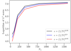
Figure 1: Choosing the function $\operatorname*{sgn}(x)$ or $\tanh(x)$ in the mobility (56) leads to different behavior as $\epsilon\to 0$, $N_{x}\to+\infty$. Above, we consider the spatially discrete mobility for height profile $h(x)=\sin(x)$. Left: For the original mobility, with $\operatorname*{sgn}(x)$, even when $\epsilon\to 0$ slowly as $N_{x}\to+\infty$, the $L^{1}$ norm of the mobility diverges. Right: Approximating with $\tanh(10x)$ allows us to send $\epsilon\to 0$ rapidly as $N_{x}\to+\infty$, while preserving a uniform bound on the $L^{1}$ norm of the mobility.

Finally, in our simulations, we sometimes approximate $\operatorname*{sgn}(x)$ in the definition of the mobility with $\tanh(10x)$. In order to achieve accurate facet formation, we must strike a balance between choosing the spatial discretization $N_{x}$ large and the mobility regularization parameter $\epsilon>0$ small. As illustrated in Figure 1, the original $\operatorname*{sgn}(x)$ function is extremely sensitive to small choices of $\epsilon$, which quickly cause the $L^{1}$ norm of the mobility to become unbounded as $\epsilon\to 0,N_{x}\to+\infty$, going against the assumption in our convergence result for the PDHG method, Theorem 3.4, which was proved for fixed $\epsilon>0$. On the other hand, the $\tanh(10x)$ approximation allows us to refine $\epsilon$ and $N_{x}$ simultaneously, while keeping the $L^{1}$ norm of the mobility bounded. A thorough analysis of these limits is related to the question of existence of solutions to the crystal surface evolution equation, and we leave a detailed study to future work.

5 Numerical Results

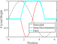
$h_{\text{sine}}(x)\ =\ \ \ \sin(x)$

$h_{\text{jump}}(x)=\begin{cases}\sin(2x)&x\in(\pi/2,3\pi/2)\\ 0&\text{otherwise}\end{cases}$

$h_{\text{facet}}(x)=\begin{cases}\sin(2(x-\pi/2))&x\in\left(\frac{\pi}{2},\frac{3\pi}{4}\right)\\ 1&x\in(3\pi/4,5\pi/4)\\ \cos(2(x-5\pi/4))&x\in(5\pi/4,3\pi/2)\\ 0&\text{otherwise}\end{cases}$

Figure 2: Choices of initial data.

In this section, we present a range of numerical examples illustrating the performance of the proposed algorithm. In each test, we consider the stopping criteria $\|(h^{(m+1)}-h^{(m)},\phi^{(m+1)}-\phi^{(m)})\|<\delta$, where we take the threshold $\delta=5\times 10^{-6}$. Unless otherwise specified, the outer time step for the semi-implicit scheme $h^{n}$ is chosen to be $\tau=T/10$, where $T$ is the final computational time, so that $N_{t}=10$. In order to ensure that the matrix inverse in the definition of $h^{(m+1)}$, equation (55), is well defined, we choose $\lambda$ sufficiently large so that $\frac{\tau}{\lambda}\|\mathsf{A}\mathsf{D}^{t}\mathsf{D}\|<1$. In the following examples, we choose $\sigma=5\times 10^{-4},\lambda=500$ for all $N_{x}$. We consider three choices of initial data, as shown in Figure 2.

Sinuoidal                        Jump Discontinuities                          Facet

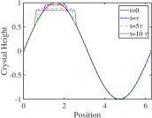
Figure 3: Dynamics of crystal surface evolution equation for different choices of initial data. Near maxima, flat facets form and expand outward, while minima remain stationary.

In Figure 3, we display the dynamics of the crystal surface evolution equation for each choice of initial data. We chose $\epsilon=0.04$, $N_{x}=200$ in each of these calculations, letting $T=10^{-2}$ in the case of the Sinusoidal and the Facet dynamics and $T=10^{-3}$ for the Jump dynamics. Near the maxima, flat facets expand outward like a free boundary type solution, while the minimum is stationary, as predicted in [29].

Sinuoidal                        Jump Discontinuities                          Facet
 

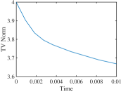
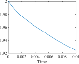
Figure 4: Top row: The total variation energy decreases in time along numerical solutions, reflecting the underlying gradient flow structure. Bottom row: The $L^{1}$ norms of the mobility $M(h)$ and the reciprocal of the mobility $1/M(h)$ are large, but remain bounded along the flow.

In Figure 4, we analyze properties of the numerical method, under the same choices of parameters as in Figure 3. In the top row, we show the decrease in the discrete TV norm $\|\mathsf{D}h\|_{1}$ in time along solutions of the equation, reflecting the gradient flow structure of the equation. In the bottom row, we plot the $L^{1}$ norms of the mobility $M(h)$ and its reciprocal $1/M(h)$. A key assumption in our convergence result for the PDHG method, Theorem 3.4, is that both remain bounded, uniformly in the spatial discretization. We can see in the above simulations that, while these norms are very large, they indeed remain bounded along the flow.

$\operatorname*{sgn}(x)$                               $\tanh(10x)$                                $\tanh(10x)$

Figure 5: We compare the dynamics of the mobility given by equation (56) with a modified mobility, in which $\operatorname*{sgn}(x)$ is replaced by $\tanh(10x)$. While the original mobility more accurately prevents facet formation at the local minimum, the modified mobility leads has smaller $L^{1}$ norm and requires fewer iterations to converge.

In Figure 5, we compare two different choices of mobility: equation (56) and a modified mobility, replacing $\operatorname*{sgn}(x)$ with $\tanh(10x)$. In both cases, we take $\epsilon=.04$. On one hand, the modified mobility has the benefit of drastically decreasing the $L^{1}$ norm of the mobility and its reciprocal: compare the plot on the right to the bottom left plot of Figure 4. The method also requires fewer iterations to meet the stopping criteria. On the other hand, the modified mobility allows for slightly more movement and facet formation at the minimum, which goes against the predicted dynamics of the original equation: compare the plot on the left with the plot in the middle.

Figure 6: Left: Log-Log plot of relative $L^{1}$ error vs. spatial grid size. Middle: Log-Log plot of relative $L^{1}$ error vs. external time step. Right: Comparison of number of time steps required to meet stopping criteria for either $\dot{H}^{1}$ or $L^{2}$ penalization. We observe superior performance for the $\dot{H}^{1}$ penalization, especially as the spatial grid is refined.

Finally, in Figure 6, we analyze the rate of convergence of our method. We consider sinusoidal initial data with the modified mobility, replacing $\operatorname*{sgn}(x)$ with $\tan(10x)$, $\epsilon=.05$ and $T=10^{-4}$. On the left, we examine how the relative $L^{1}$ error depends on the number of spatial gridpoints $N_{x}$ for a fixed temporal discretization, $N_{t}=10$. For $N_{x}=16,32,64,128,256,512$, we plot $\|h(N_{x})-h(2N_{x})\|_{L^{1}}$. We observe slightly sublinear convergence, in line with the low spatial regularity of our solutions.

In the middle plot, we examine how the relative $L^{1}$ error scales with the external time step, used to define the semi-implicit scheme $h^{n}$ via $\tau=T/N_{t}$, for a fixed spatial discretization $N_{x}=256$. For $N_{t}=5,10,20,40,80$, we plot $\|h(N_{t})-h(2N_{t})\|_{L^{1}}$. We observe approximately first order convergence, in agreement with the interpretation of our scheme as a semi-implicit version of the minimizing movements scheme, which can be thought of as a generalized Euler method.

In the right plot, we illustrate the importance of the choice of norms in our PDHG algorithm, as explained in Remark 3.2. At the fully discrete level, existing work [9] ensures that the PDHG algorithm would converge, even if the norm penalization in the definition of $h^{(m+1)}$ was changed from a $\dot{H}^{1}$ norm to a $L^{2}$ norm. At the level of Algorithm 1, this would amount to modifying the computation of $h^{(m+1)}$ as follows:

(57) $$h^{(m+1)}=\left(\mathsf{I}+\frac{\lambda}{\tau}\mathsf{A}^{-1}(\cdot-h^{n})\right)^{-1}\left(h^{(m)}-\lambda\mathsf{D}^{t}\phi^{(m)}\right).$$

On one hand, to invert the matrix in the above formula, we need $\frac{\tau}{\lambda}\|\mathsf{A}\|<1$. On the other hand, existing convergence results on PDHG require $\lambda\sigma\|\mathsf{D}^{t}\mathsf{D}\|<1$, where $\|\mathsf{D}^{t}\mathsf{D}\|\to+\infty$ as the spatial grid is refined. These requirements lead to significant tension regarding the size of $\lambda$. In contrast, when choosing the $\dot{H}^{1}$ norm to penalize the primal variables in our PDHG algorithm, the analogue of the constraint $\lambda\sigma\|\mathsf{D}^{t}\mathsf{D}\|<1$ is simply $\lambda\sigma<1$, since the gradient is a bounded operator on $\dot{H}^{1}$. Thus, our method avoids this source of tension in the definition of the inner time steps $\lambda,\sigma$.

This discussion is born out numerically in the right plot above, in which we compare the number of iterations required for each method as the spatial grid is refined, $N_{x}=32,64,124,250,500,750$. We consider $T=10^{-6}$ external time steps, setting $\sigma=5\times 10^{-5}$, $\lambda=5\times 10^{-5}$ for the $L^{2}$ algorithm (the largest we could take to allow convergence for the $L^{2}$ Algorithm to still converge at all scales) and $\sigma=5\times 10^{-4}$, $\lambda=500$ for our $\dot{H}^{1}$ algorithm, Algorithm 1.

References

• [1] D. M. Ambrose. The radius of analyticity for solutions to a problem in epitaxial growth on the torus. Bulletin of the London Mathematical Society, 51(5):877–886, 2019.
• [2] L. Ambrosio, N. Gigli, and G. Savaré. Gradient flows in metric spaces and in the space of probability measures. Lectures in Mathematics ETH Zürich. Birkhäuser Verlag, Basel, second edition, 2008.
• [3] H. Bonzel and E. Preuss. Morphology of periodic surface profiles below the roughening temperature: aspects of continuum theory. Surface science, 336(1-2):209–224, 1995.
• [4] W.-K. Burton, N. Cabrera, and F. Frank. The growth of crystals and the equilibrium structure of their surfaces. Philosophical Transactions of the Royal Society of London. Series A, Mathematical and Physical Sciences, 243(866):299–358, 1951.
• [5] C. Cancès, T. O. Gallouët, and G. Todeschi. A variational finite volume scheme for Wasserstein gradient flows. arXiv preprint arXiv:1907.08305, 2019.
• [6] G. Carlier, V. Duval, G. Peyré, and B. Schmitzer. Convergence of entropic schemes for optimal transport and gradient flows. SIAM Journal on Mathematical Analysis, 49(2):1385–1418, 2017.
• [7] J. A. Carrillo, K. Craig, L. Wang, and C. Wei. Primal dual methods for Wasserstein gradient flows. arXiv preprint arXiv:1901.08081, 2019.
• [8] J. A. Carrillo, P. Laurençot, and J. Rosado. Fermi–Dirac–Fokker–Planck equation: Well-posedness & long-time asymptotics. Journal of Differential Equations, 247(8):2209–2234, 2009.
• [9] A. Chambolle and T. Pock. On the ergodic convergence rates of a first-order primal–dual algorithm. Mathematical Programming, 159(1-2):253–287, 2016.
• [10] C. M. Elliott and H. Garcke. On the Cahn–Hilliard equation with degenerate mobility. Siam journal on mathematical analysis, 27(2):404–423, 1996.
• [11] Y. Gao, A. E. Katsevich, J.-G. Liu, J. Lu, and J. L. Marzuola. Analysis of a fourth order exponential pde arising from a crystal surface jump process with Metropolis-type transition rates. arXiv preprint arXiv:2003.07236, 2020.
• [12] Y. Gao, J.-G. Liu, J. Lu, and J. L. Marzuola. Analysis of a continuum theory for broken bond crystal surface models with evaporation and deposition effects. Nonlinearity, 33:3816–3845, 2020.
• [13] M.-H. Giga and Y. Giga. Very singular diffusion equations: second and fourth order problems. Japan journal of industrial and applied mathematics, 27(3):323–345, 2010.
• [14] Y. Giga and R. V. Kohn. Scale-invariant extinction time estimates for some singular diffusion equations. Discrete Contin. Dyn. Syst, 30(2):509–535, 2011.
• [15] Y. Giga, H. Kuroda, and H. Matsuoka. Fourth-order total variation flow with Dirichlet condition: characterization of evolution and extinction time estimates. Hokkaido University Preprint Series in Mathematics, 1064:1–36, 2015.
• [16] R. Granero-Belinchón and M. Magliocca. Global existence and decay to equilibrium for some crystal surface models. arXiv preprint arXiv:1804.09645, 2018.
• [17] E. Gruber and W. Mullins. On the theory of anisotropy of crystalline surface tension. Journal of Physics and Chemistry of Solids, 28(5):875–887, 1967.
• [18] B. He and X. Yuan. Convergence analysis of primal-dual algorithms for a saddle-point problem: from contraction perspective. SIAM Journal on Imaging Sciences, 5(1):119–149, 2012.
• [19] T. Ihle, C. Misbah, and O. Pierre-Louis. Equilibrium step dynamics on vicinal surfaces revisited. Physical Review B, 58(4):2289, 1998.
• [20] M. Jacobs, F. Léger, W. Li, and S. Osher. Solving large-scale optimization problems with a convergence rate independent of grid size. SIAM Journal on Numerical Analysis, 57(3):1100–1123, 2019.
• [21] R. Jordan, D. Kinderlehrer, and F. Otto. The variational formulation of the Fokker-Planck equation. SIAM J. Math. Anal., 29(1):1–17, 1998.
• [22] R. Kobayashi and Y. Giga. Equations with singular diffusivity. Journal of statistical physics, 95(5-6):1187–1220, 1999.
• [23] R. V. Kohn and H. M. Versieux. Numerical analysis of a steepest-descent pde model for surface relaxation below the roughening temperature. SIAM journal on numerical analysis, 48(5):1781–1800, 2010.
• [24] B. Krishnamachari, J. McLean, B. Cooper, and J. Sethna. Gibbs-Thomson formula for small island sizes: Corrections for high vapor densities. Physical Review B, 54(12):8899, 1996.
• [25] J. Krug, H. Dobbs, and S. Majaniemi. Adatom mobility for the solid-on-solid model. Zeitschrift für Physik B Condensed Matter, 97(2):281–291, 1995.
• [26] W. Li, J. Lu, and L. Wang. Fisher information regularization schemes for Wasserstein gradient flows. Journal of Computational Physics, page 109449, 2020.
• [27] M. Liero and A. Mielke. Gradient structures and geodesic convexity for reaction–diffusion systems. Philosophical Transactions of the Royal Society A: Mathematical, Physical and Engineering Sciences, 371(2005):20120346, 2013.
• [28] S. Lisini, D. Matthes, and G. Savaré. Cahn–Hilliard and thin film equations with nonlinear mobility as gradient flows in weighted-Wasserstein metrics. Journal of Differential Equations, 253(2):814–850, 2012.
• [29] J.-G. Liu, J. Lu, D. Margetis, and J. L. Marzuola. Asymmetry in crystal facet dynamics of homoepitaxy by a continuum model. Physica D: Nonlinear Phenomena, 393:54–67, 2019.
• [30] J.-G. Liu and R. M. Strain. Global stability for solutions to the exponential pde describing epitaxial growth. Interfaces and Free Boundaries, 21:51–86, 2019.
• [31] J.-G. Liu and X. Xu. Existence theorems for a multidimensional crystal surface model. SIAM Journal on Mathematical Analysis, 48(6):3667–3687, 2016.
• [32] J.-G. Liu and X. Xu. Analytical validation of a continuum model for the evolution of a crystal surface in multiple space dimensions. SIAM Journal on Mathematical Analysis, 49(3):2220–2245, 2017.
• [33] D. Margetis and R. V. Kohn. Continuum relaxation of interacting steps on crystal surfaces in 2+1 dimensions. Multiscale Modeling & Simulation, 5(3):729–758, 2006.
• [34] J. L. Marzuola and J. Weare. Relaxation of a family of broken-bond crystal-surface models. Physical Review E, 88(3):032403, 2013.
• [35] R. Najafabadi and D. J. Srolovitz. Elastic step interactions on vicinal surfaces of fcc metals. 1994.
• [36] H. Nessyahu and E. Tadmor. Non-oscillatory central differencing for hyperbolic conservation laws. J. Comput. Phys., 87:408–463, 1990.
• [37] I. V. Odisharia. Simulation and analysis of the relaxation of a crystalline surface. New York University, 2006.
• [38] F. Otto. The geometry of dissipative evolution equations: the porous medium equation. Comm. Partial Differential Equations, 26(1-2):101–174, 2001.
• [39] J. S. Rowlinson and B. Widom. Molecular theory of capillarity. Courier Corporation, 2013.
• [40] L. I. Rudin, S. Osher, and E. Fatemi. Nonlinear total variation based noise removal algorithms. Physica D: nonlinear phenomena, 60(1-4):259–268, 1992.
• [41] R. Shefi and M. Teboulle. Rate of convergence analysis of decomposition methods based on the proximal method of multipliers for convex minimization. SIAM Journal on Optimization, 24(1):269–297, 2014.
• [42] V. Shenoy and L. Freund. A continuum description of the energetics and evolution of stepped surfaces in strained nanostructures. Journal of the Mechanics and Physics of Solids, 50(9):1817–1841, 2002.
• [43] J. Wang and B. J. Lucier. Error bounds for finite-difference methods for Rudin–Osher–Fatemi image smoothing. SIAM Journal on Numerical Analysis, 49(2):845–868, 2011.
• [44] A. Zangwill, C. Luse, D. Vvedensky, and M. Wilby. Equations of motion for epitaxial growth. Surface science, 274(2):L529–L534, 1992.
• [45] W. P. Ziemer. Weakly differentiable functions: Sobolev spaces and functions of bounded variation, volume 120. Springer Science & Business Media, 2012.