Cosmological Forecast for non-Gaussian Statistics in large-scale weak Lensing Surveys

Abstract

Cosmic shear data contains a large amount of cosmological information encapsulated in the non-Gaussian features of the weak lensing mass maps. Weak lensing studies mostly rely on two-point statistics to constrain cosmology from cosmic shear data, that do not capture all of this information. Additional non-Gaussian information can be extracted using non-Gaussian statistics. We compare the constraining power in the $\Omega_{\mathrm{m}}-\sigma_{8}$ plane of three map-based non-Gaussian statistics with the angular power spectrum, namely; peak counts, minimum counts and Minkowski functionals. We further analyze the impact of tomography and systematic effects originating from galaxy intrinsic alignments, multiplicative shear bias and photometric redshift systematics. We forecast the performance of the statistics for a stage-3-like weak lensing survey, spanning an area of 5000 deg² and restrict ourselves to scales $\geq$ 10 arcmin to avoid baryonic effects. The study follows a forward modelling scheme to predict the statistics at different cosmologies based on N-Body simulations. We find, that in our setup, the considered non-Gaussian statistics provide tighter constraints than the angular power spectrum. The peak counts show the greatest potential, increasing the Figure-of-Merit (FoM) in the $\Omega_{\mathrm{m}}-\sigma_{8}$ plane by a factor of about 4, while the minimum counts and the Minkowski functionals yield an increase by a factor of about 2. A combined analysis using all non-Gaussian statistics in addition to the power spectrum increases the FoM by a factor of 5 and reduces the error on $S_{8}$ by $\approx$ 25%. We find that the importance of tomography is diminished when combining non-Gaussian statistics with the angular power spectrum. The non-Gaussian statistics indeed profit less from tomography and the minimum counts and Minkowski functionals add some robustness against galaxy intrinsic alignment in a non-tomographic setting. We further find that a combination of the angular power spectrum and the non-Gaussian statistics allows us to apply conservative scale cuts in the analysis, thus helping to minimize the impact of baryonic and relativistic effects, while conserving the cosmological constraining power. We make the code that was used to conduct this analysis publicly available to simplify performing such analyses in the future.

1 Introduction

The $\Lambda$CDM model succeeds to explain and predict the main observables of the Universe, including the Big Bang nucleosynthesis (see e.g. [1]), the anisotropies of the cosmic microwave background (CMB) (see e.g. [2]) and the Hubble diagram of Type Ia supernovae (see e.g. [3]). Although recent results point towards a disagreement in the value of the Hubble parameter as inferred from local measurements [4, 5, 6, 7] and from CMB studies [8, 9], the $\Lambda$CDM model remains the most successful cosmological model to date. It is based on general relativity and mainly characterized by a flat geometry, a cosmological constant $\Lambda$ and a cold dark matter (CDM) component, driving the formation of structures. To further deepen our understanding of the Universe, it is essential to provide novel measurements that are able to challenge the model and potentially discover deviations from it, that might lead to the discovery of new physics.

One way to provide such tests is given by the investigation of the cosmic shear, which is the coherent distortion of the apparent ellipticities of galaxies, caused by weak gravitational lensing (WL) by the foreground large-scale structure of the Universe [10]. These distortions are typically at the percent level. However, by measuring millions of galaxy shapes on the sky, as it is achieved by modern large scale imaging surveys, the statistical potential of the method is large. The simple theoretical description of WL, as well as its independence on galaxy biasing, are further advantages of the method [11].

The feasibility and potential of cosmic shear studies was successfully demonstrated by past surveys, such as the Canada France Hawaii Telescope Lensing Survey (CFHTLens) [12] or the Sloan Digital Sky Survey (SDSS) [13]. Putting new constraints on the cosmological model using WL is not only one of the main science goals of currently ongoing stage 3 surveys, such as the Dark Energy Survey (DES) [14], Kilo-Degree Survey (KIDS) [15] or the Hyper Suprime-Cam (HSC) [16], but also served as one of the major motivations for future stage 4 surveys such as the Large Synoptic Survey Telescope (LSST) [17] or Euclid [18].

Cosmic shear measurements are affected by a variety of systematic effects. The accessibility of small scales in cosmic shear experiments is limited due to biases arising from baryonic physics, such as radiative cooling (see e.g. [19]) or feedback effects caused by the active galactic nucleus (AGN), stellar winds or supernovae [20]. These baryonic effects are generally difficult to treat in a dark-matter-only framework, as it is commonly used in cosmic shear studies (see e.g. [20]). Galaxy intrinsic alignment, describing the gravitational interaction of galaxies with the large-scale structure, can lead to correlations of the intrinsic ellipticities of the source galaxies and a contamination of the cosmic shear signal (see e.g. [21]). This effect is similarly difficult to account for as baryonic effects. In addition to systematic effects arising from unaccounted physics, biases can arise due to imperfections in the measurement and data reduction process. Some of these effects can be taken into account by introducing a multiplicative shear bias (see e.g. [22]). In particular, inaccuracies in the measurement of the redshift distribution of the source galaxies can bias cosmic shear measurements. These photometric redshift errors cannot be modelled as a multiplicative bias component and are therefore treated separately (see e.g. [23]). Further higher-order systematic effects include magnification bias, source-lens clustering or reduced shear bias, for example.

As the number of measured galaxy shapes increases with the observed cosmological volume, the statistical error in the measurements decreases and the correct understanding and treatment of these systematic effects becomes more pressing. Also, with the advent of tensions between the inferred values of cosmological parameters from different cosmological probes, finding new ways to improve the robustness of WL measurements against these systematic effects becomes essential. An important example is the disagreement in the value of the amplitude of density fluctuations $\sigma_{8}$, between WL surveys and the results from CMB experiments like Planck [9], with the WL studies yielding consistently lower values [24].

Up to now, the shear two-point correlation function and its Fourier counterpart, the angular power spectrum, served as the main WL observables. While ongoing surveys like KIDS, DES and HSC make major contributions to the understanding of how systematics affect those two-point statistics, we are taking a complementary route by investigating the robustness of alternative, non-Gaussian WL observables to the major effects driving the systematic uncertainty.

In the case of a homogeneous, isotropic Gaussian random field two-point statistics are sufficient summary statistics. However, due to the non-linear nature of gravitational collapse, this assumption is not valid on small scales and at late times, as the density field becomes non-Gaussian. Therefore, two-point statistics are insufficient to fully describe the matter density field and additional statistics ought to be considered (see e.g. [25]). Additionally, each statistic is affected differently by systematic effects. Hence, a combination of multiple statistics can allow for a better calibration and understanding of the different systematics and ultimately improve the robustness of the measurement.

A variety of statistics optimized to capture the non-Gaussian information of the cosmic shear signal was previously developed and tested. A natural extension after the study of two-point statistics is to consider higher-order statistics, such as three-point correlation functions [26] or the bispectrum [27], which has been shown to capture complementary information and significantly improve parameter constraints [28]. A computationally less demanding way to access the additional information of the cosmic shear signal is provided by the moments of WL mass maps. This method was first studied by [29] and a recent study demonstrates its potential for the Year 3 data of the DES [30]. Other non-Gaussian statistics include for example, higher moments (see e.g. [31]) or the PDF of the convergence field [32]. In this work, we forecast the performance of peak counts (PC) (see Section 2.2), minimum counts (MC) (see Section 2.3) and Minkowski Functionals (MFs) (see Section 2.4).

It was shown, by [33] that the count of peaks on mass maps can be used to constrain cosmology. The method was applied to CFHTLens data by [34] and to the DES Science Verification data by [35]. The potential of using the lensing signal around local minima of WL mass maps was demonstrated by [36] and [37], using the DES Science Verification data. The counts of such local minima of the mass maps can also serve as a mean to constrain cosmology [38]. While the PC and MC focus on extracting information from local features of the lensing signal, it was shown, that MFs can probe cosmology using the global topology of mass maps [39]. The method was applied to CFHTLens data by [40].

The primary goal of this work is to forecast and compare the resulting constraining power on the total matter density $\Omega_{\mathrm{m}}$ and the fluctuation amplitude $\sigma_{8}$ when using the PC, MC, MFs, as well as the angular power spectrum and different combinations of these statistics. We forecast the performance, using a simulated stage-3-like WL survey.

Additionally, we investigate the robustness of the statistics against the three major WL systematics; galaxy intrinsic alignment, multiplicative shear bias and photometric redshift error (see Section 3.6). The two-point statistics are affected by these effects. In particular, galaxy intrinsic alignment has been shown to potentially bias the cosmological constraints and increase systematic uncertainty, with the two-point statistics being unable to constrain galaxy intrinsic alignment in a non-tomographic setup (see e.g. [41]). While the use of tomography improves the constraints on galaxy intrinsic alignment considerably and helps to reclaim a large part of the otherwise lost constraining power, it requires knowledge of the redshift distribution of the source galaxy population, obtained through photometric redshift estimates [12]. With photometric redshift estimation being a source of systematic biases and uncertainty itself, we investigate the possibility of non-Gaussian statistics being able to constrain galaxy intrinsic alignment in a non-tomographic analysis.

While a lot of information about the large-scale structure can be obtained from very large- and small-scale features of the cosmic shear field, additional systematic effects become relevant on these scales (e.g. relativistic corrections on large scales [42] or baryonic corrections on small scales [20]). This limits the range of scales that can be safely considered in cosmic shear analyses. We study, whether the addition of non-Gaussian statistics to the analysis can provide an alternative route to using such scales by providing additional constraining power.

Contrarily to the two-point statistics, non-Gaussian statistics have the disadvantage that making analytical predictions from theory for different cosmologies is often difficult, complicating the inference of cosmological constraints. One approach is to rely on analytical approximations to predict the statistics at different cosmologies, as it is done for peak counts in [43] or for Minkowski functionals in [44], for example. We take a different route and circumvent this problem in our analysis by relying on a forward modelling approach, predicting the statistics for different cosmologies based on a suite of N-Body simulations and therefore avoiding the necessity of analytical predictions of the statistics. However, this approach has the disadvantage that it comes with a higher computational cost and requires to setup a simulation pipeline. Hence, we develop and distribute a code framework aimed at simplifying this kind of WL analysis.

We start with a summary of the most important properties of WL and an introduction of the studied statistics in Section 2. In Section 3, we guide the reader through our analysis and introduce the ingredients and codes used in this work. We present the simulated, non-tomographic statistics and their cosmology-dependence in Section 4 and follow up with an investigation on their cosmological constraining power and robustness to the studied systematics in Section 5. The work concludes with the main findings and a short outlook on possible extensions in Section 6.

2 Weak Lensing Statistics

The phenomenon of gravitational lensing refers to the deflection of photons, traveling from a distant source towards an observer. The deflection is caused by the foreground density fluctuations along the line of sight. In the context of gravitational lensing the foreground density fluctuations act like a medium with variable refractive index for the propagating photons, causing their deflection. Gravitational lensing can cause the appearance of an extended background object to be distorted. In the regime of WL, where the distortions are small, the change of the shape of a lensed object can be broken down into two parts; the convergence $\kappa$, describing an isotropic magnification of the object and the shear $\gamma=(\gamma_{1},\gamma_{2})$ denoting an anisotropic stretching (see e.g. [45, 10]).

In cosmic shear studies one observes the percent level distortions of the ellipticities of distant galaxies, caused by the lensing due to the foreground large-scale structure of the Universe. Therefore, by measuring the fields $\gamma$ and $\kappa$ on the sky, which are related to the gravitational potential $\Phi$ that is induced by the large-scale structure, one can learn about the distribution of matter in the local Universe. Due to this connection, cosmic shear is mostly sensitive to the cosmological parameters describing the matter distribution of the local Universe, namely; the matter density $\Omega_{\mathrm{m}}$, the fluctuation amplitude $\sigma_{8}$, the dark energy density $\Omega_{\Lambda}$ and the dark energy equation-of-state parameter $w$ (see e.g. [46]).

The two fields $\kappa$ and $\gamma$ are not independent of each other, but they are linked via the gravitational potential $\Phi$ [47]. This connection can be used to derive $\kappa$ from $\gamma$ and vice versa. The most widely used method to do so is the Kaiser-Squires mass-mapping method [48]. This approach relies on approximating part of the celestial sphere as a plane. While this assumption is valid for small scale surveys like CFHTLens, it is not applicable for ongoing stage 3 surveys like DES [14] or stage 4 surveys like LSST [17]. Therefore, we rely on a spherical extension of this method introduced in [47].

Being defined as fields on the sphere, $\kappa$ and $\gamma$ can be decomposed in the basis of spherical harmonics as

$$\kappa(\theta,\phi) =\sum_{\ell=0}^{\infty}\sum_{m=-\ell}^{\ell}\tensor[_{0}]{\hat{\kappa}}{{}_{\ell m}}\cdot\tensor[_{0}]{Y}{{}_{\ell m}}(\theta,\phi),$$ (2.1)

$$\gamma(\theta,\phi) =\sum_{\ell=0}^{\infty}\sum_{m=-\ell}^{\ell}\tensor[_{2}]{\hat{\gamma}}{{}_{\ell m}}\cdot\tensor[_{2}]{Y}{{}_{\ell m}}(\theta,\phi),$$ (2.2)

where $\tensor[_{0}]{Y}{{}_{\ell m}}(\theta,\phi)$ are the spin-0 and $\tensor[_{2}]{Y}{{}_{\ell m}}(\theta,\phi)$ the spin-2 spherical harmonics, respectively. The coefficients $\tensor[_{0}]{\hat{\kappa}}{{}_{\ell m}}$ can be calculated from the ${}_{2}\hat{\gamma}_{\ell m}$ coefficients via the relation

$${}_{0}\hat{\kappa}_{\ell m}=D_{\ell}^{-1}\cdot\tensor[_{2}]{\hat{\gamma}}{{}_{\ell m}},$$ (2.3)

using the kernel

$$D_{\ell}=\frac{-1}{\ell(\ell+1)}\sqrt{\frac{(\ell+2)!}{(\ell-2)!}}.$$ (2.4)

This relation can be obtained by relating the coefficients via the gravitational potential $\Phi$ [47]. The inverse relation can also be used to reconstruct the $\gamma$ field from the $\kappa$ field in the same fashion. This approach was already used successfully in [49] and [31], for example.

2.1 Angular Power Spectrum (CLs)

The angular two-point correlation function and its Fourier analogue, the angular power spectrum (CLs), served as the main statistics for the extraction of information from cosmic shear data in past WL surveys (see e.g. [15, 12]). The angular two-point correlation function

$$\xi(|\vec{x}_{1}-\vec{x}_{2}|=\theta)=\left\langle F(\vec{x}_{1}),F(\vec{x}_{2})\right\rangle$$ (2.5)

describes the expected value of a random field $F$ at a fixed angular distance $\theta$ from a random point $\vec{x}_{1}$, given that a certain value of the field was measured at that point [50]. Given a decomposition of the field $F$ in the basis of spherical harmonics as

$$F=\sum_{\ell=0}^{\infty}\sum_{m=-\ell}^{\ell}a_{lm}\tensor[]{Y}{{}_{\ell m}}(\theta,\phi),$$ (2.6)

one can define the angular power spectrum $C_{\ell}$ of the field $F$ as

$$C_{\ell}=\frac{1}{2\ell+1}\sum_{m=-\ell}^{\ell}|a_{lm}|^{2}.$$ (2.7)

The convergence field $\kappa$ is commonly decomposed into a curl-free component $\kappa_{\mathrm{E}}$ and a divergence-free component $\kappa_{\mathrm{B}}$ as

$$\kappa(\theta,\phi)=\kappa_{\mathrm{E}}+i\kappa_{\mathrm{B}}=\sum_{\ell=0}^{\infty}\sum_{m=-\ell}^{\ell}(\tensor[_{0}]{\hat{\kappa}}{{}_{\mathrm{E},\ell m}}+i\tensor[_{0}]{\hat{\kappa}}{{}_{\mathrm{B},\ell m}})\enspace\tensor[_{0}]{Y}{{}_{\ell m}}(\theta,\phi),$$ (2.8)

allowing the decomposition of the angular power spectrum into three separate terms

$$C_{\ell}^{\mathrm{EB}} =\frac{1}{2\ell+1}\sum_{m=-\ell}^{\ell}\tensor[_{0}]{\hat{\kappa}}{{}_{\mathrm{E},\ell m}}\tensor[_{0}]{\hat{\kappa}}{{}_{\mathrm{B},\ell m}^{*}},$$ (2.9)

$$C_{\ell}^{\mathrm{EE}} =\frac{1}{2\ell+1}\sum_{m=-\ell}^{\ell}|\tensor[_{0}]{\hat{\kappa}}{{}_{\mathrm{E},\ell m}}|^{2},$$ (2.10)

$$C_{\ell}^{\mathrm{BB}} =\frac{1}{2\ell+1}\sum_{m=-\ell}^{\ell}|\tensor[_{0}]{\hat{\kappa}}{{}_{\mathrm{B},\ell m}}|^{2}.$$ (2.11)

The vast majority of the cosmological signal is carried by the E-modes ($C_{\ell}^{EE}$), while B-modes ($C_{\ell}^{\mathrm{BB}}$) mostly arise from systematics in the shear-calibration process or object selection biases. EB-modes ($C_{\ell}^{\mathrm{EB}}$) are generated via mode mixing due to masking effects. Given that most of the cosmological signal is captured by the E-modes, we neglect EB-, and B-modes in this study. The angular power spectrum can also be related to an integral over the matter power spectrum of the Universe [51]. Using the Limber and small-angle approximations, the computation can be sped up significantly and allows to obtain approximative predictions for the CLs for different cosmologies (see e.g. [45, 52]). We note that we do not require to denoise the measurement CL signal in this work, as it is commonly done in analyses where the CL signal needs to be compared to a theory prediction. In a simulation-based approach, as it is used in this work, the measurement and the predictions of the signal at different cosmologies both contain a statistically equivalent noise component (see Section 3).

2.2 Peak Counts (PC)

The idea that massive dark matter halos could imprint themselves onto mass maps as local maxima, so called peaks, was pioneered by the works of [48, 53, 54]. While peaks were first studied mainly as a mean to detect massive clusters from mass maps (see e.g. [55]), it was found later that they can also serve directly as a cosmological probe (see e.g. [56, 57]). We detect peaks from the pixelized mass maps by comparing each pixel to its direct neighbors. A pixel is regarded as a peak if its value is higher than all of the values of its neighboring pixels. We bin the found peaks as a function of their convergence value. In addition to counting peaks, the consideration of further peak statistics, such as peak-profiles or peak-correlation functions can help to improve cosmological constraints [58]. In this work we only study peak counts (PC) and we leave the exploration of peak-profiles and peak-correlation functions to further studies. While using peaks instead of CLs has the advantage of becoming more sensitive to the non-Gaussian features of the maps [59], it comes at the cost of a complicated and at most approximative analytical prediction of the PC for different cosmologies (see e.g. [43]). We avoid having to rely on such approximative predictions by using a forward modelling approach and predict the PC for different cosmologies using simulations, as described in Section 3.

2.3 Minimum Counts (MC)

While the idea of using peaks as a cosmological probe became popular in recent years, using counts of local minima of the mass maps to infer cosmology received less attention, although the lensing signal around such under-dense regions was already proposed as a way to provide insight into interesting physics, such as modified gravity (see e.g. [60, 61]). While peaks are sensitive to over-densities of the matter distribution, local minima probe its under-densities. Hence, they can potentially probe complementary information. Another aspect that makes local minima an interesting probe, is that they target regions with small amounts of baryonic matter. It was shown, that local minima suffer less from effects related to baryonic physics than other statistics [38]. The identification of local minima of the projected WL signal, as compared to finding under-dense regions from the three dimensional matter distribution, has the advantage that one does not require a complicated void identification scheme nor a void tracer, such as halos [38]. Our detection of local minima is similar to the detection of peaks. We record a pixel as a minimum, if the recorded value is smaller than the values recorded for all of its direct neighbors. The same kinds of summary statistics as for peaks can be used for minima as well; minimum counts (MC), the profiles around minima and the correlation function of minima. We only study the MC and leave the investigation of the other statistics to future studies.

2.4 Minkowki Functionals (MFs)

Minkowski Functionals (MFs) are mathematical descriptors of the global topology of continuous, stochastic fields. They capture information contained in the n-point correlators of the field of any order n, which makes them natural probes of non-Gaussianity [62]. For a two-dimensional field, such as a mass map, there exist only three MFs, dubbed $V_{0}$, $V_{1}$ and $V_{2}$. As the MFs are scale-dependent, they are calculated for a number of different excursion sets $Q_{t}$ of the field. The excursion set $Q_{t}$ is formed by the region of the field where the field value exceeds the threshold $t$. Hence, the MFs are functions of $t$. The three MFs for a two-dimensional field are defined as

$$V_{0}(t) =\int_{Q_{t}}\mathrm{d}a,$$ (2.13)

$$V_{1}(t) =\frac{1}{4}\int_{\partial Q_{t}}\mathrm{d}l,$$ (2.14)

$$V_{2}(t) =\frac{1}{2\pi}\int_{\partial Q_{t}}\mathcal{K}\thinspace\mathrm{d}l,$$ (2.15)

where $\mathrm{d}a$ and $\mathrm{d}l$ are the surface and line elements of the excursion sets $Q_{t}$ and $\mathcal{K}$ is the local geodesic curvature. Geometrically speaking, $V_{0}$ describes the area, $V_{1}$ the perimeter and $V_{2}$ the Euler characteristic of the excursion sets [63]. Since the MFs can be analytically computed for a Gaussian random field, they are commonly used to quantify the deviation from Gaussianity of a field [64]. On the other hand, no exact, analytical prediction can be made for non-Gaussian fields. Commonly, the non-Gaussian part of the MFs is treated as a perturbation of the Gaussian part and expanded in a perturbation series (see e.g. [63, 44, 65]). If the non-Gaussianity of the field is weak, the series converges and can be truncated to obtain an approximative prediction for the MFs. In the presence of strong non-Gaussianity though, as it is typically the case for mass maps, the series does not converge [65]. In our forward modelling approach, we are not affected by this problem, since we do not require to make analytical predictions for the MFs at different cosmologies. Following [65], we measure the MFs from the mass maps directly as

$$V_{0}(t) =\frac{1}{Q_{t}}\int_{Q_{t}}\Theta(\kappa(\vec{x})-t)\thinspace\mathrm{d}x\thinspace\mathrm{d}y,$$ (2.16)

$$V_{1}(t) =\frac{1}{4Q_{t}}\int_{Q_{t}}\delta(\kappa(\vec{x})-t)\sqrt{(\partial_{x}\kappa)^{2}+(\partial_{y}\kappa)^{2}}\thinspace\mathrm{d}x\thinspace\mathrm{d}y,$$ (2.17)

$$V_{2}(t) =\frac{1}{2\pi Q_{t}}\int_{Q_{t}}\delta(\kappa(\vec{x})-t)\frac{2\partial_{x}\kappa\partial_{y}\kappa\partial_{x}\partial_{y}\kappa-(\partial_{x}\kappa)^{2}\partial_{y}^{2}\kappa-(\partial_{y}\kappa)^{2}\partial_{x}^{2}\kappa}{(\partial_{x}\kappa)^{2}+(\partial_{y}\kappa)^{2}}\thinspace\mathrm{d}x\thinspace\mathrm{d}y,$$ (2.18)

where $\Theta$ and $\delta$ denote the Heaviside step function and the Dirac delta function, respectively. The gradients are calculated numerically on a pixel level.

3 Method

In this work, we are forecasting the constraining power of different map-based statistics for a stage-3-like WL survey and we investigate their robustness to systematic effects. In the forward modelling framework that we have chosen to conduct this study we require a stage-3-like mock survey and a suite of N-Body simulations spanning a range of different cosmologies. Using these two ingredients we simulate mass maps with the same survey properties as the mock survey but with different cosmological signals, by drawing the noise signal from the mock survey and adding it to the simulated cosmological signal. These maps allow us to predict the statistics and calculate the likelihood at different cosmologies enabling us to use Bayesian inference to find the parameter constraints.
In the following we describe the different steps involved in this process in greater detail. Our analysis is built on the work of [49], where a similar approach was used to investigate the constraining power of the peak abundance function for a 2000 deg² survey.

3.1 Mock Survey

We generate a stage-3-like mock survey by randomly drawing galaxy positions on the sky. The positions are drawn within a square patch (in a cylindrical projection) of 5000 deg² until the target galaxy density of 5 arcmin^-2 is reached. For each galaxy, we randomly draw its ellipticity $e$ from a probability density given as

$$\mathrm{Prob}(|e|)\propto(|e|+0.01)^{-4}[1-\exp(-23|e|^{4})].$$ (3.1)

This function was chosen to fit the distribution of the galaxy ellipticities recorded in [66] (hereafter T18). The functional form was proposed by [67] and used successfully in [49]. The individual ellipticity components $e_{1}$ and $e_{2}$ are obtained by random rotation of the ellipticity as

$$e_{1} =\Re{[|e|\exp(i\phi)]},$$

$$e_{2} =\Im{[|e|\exp(i\phi)]},$$ (3.2)

where the angle $\phi$ is drawn uniformly from the interval $[0,2\pi[$. We truncate the ellipticity distribution at a value of 1.5 in order to avoid extreme outlier events. Note that the mock survey does not need to contain a cosmological signal, since it is only used as a source for the noise component (see Section 3.3).

The redshift $z$ of the galaxies is drawn from a Smail distribution [68] parameterized as

$$\mathrm{Prob}(z)\propto z^{1.5}\exp\left(-\left[\frac{z}{0.31}\right]^{1.1}\right),$$ (3.3)

where we fitted the parameters, such that the global redshift distribution $n(z)$ of the simulated galaxies resembles the redshift distribution found in T18. Since we also aim to compare parameter constraints in a tomographic setup, we additionally require to assign each galaxy to a tomographic bin. We perform this division, such that each tomographic bin contains the same number of galaxies, according to the scheme used in [69]. Following the analysis of T18 we use 4 tomographic bins for the tomographic setup. The global redshift distribution $n(z)$ of the simulated galaxies, as well as the distributions of the 4 tomographic bins is shown in Figure 1.

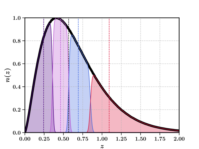
Figure 1: Global redshift distribution $n(z)$ of the simulated galaxies in the mock survey as well as the distributions of the 4 tomographic bins. The global redshift distribution as indicated by the black curve was fitted to the redshift distribution found by T18. The dashed, vertical lines indicate the median redshift of the global and tomographic distributions, respectively. The distributions are normalized.

3.2 N-Body Simulations

We use the publicly available N-Body code PKDGRAV3 [70] to sample a grid of cosmologies in the $\Omega_{\mathrm{m}}-\sigma_{8}$ plane. PKDGRAV3 is a dark-matter-only, full-tree code that uses a fast multipole expansion to calculate the gravitational force, achieving a linearly increasing run time in the number of particles. The code also features GPU-acceleration.

The simulations used in this work were performed using $768^{3}$ particles, a box with a side-length of 900 Mpc/h and periodic boundary conditions. Depending on cosmology, we replicate the box up to 14 times along each dimension ($14^{3}$ replications in total), in order to sample a large enough cosmological volume, such that we can cover the necessary redshift range (up to $z=3.0$). Note that such a replication under-predicts the variance of the simulations on large scales. However, since we use a lower scale cut of $\ell=100$ the results are not affected by the replication (see Section 4.1). The initial conditions for the simulations are generated at $z=99.0$. The resulting particle positions are returned in 87 shells taken from redshift $z=3.0$ up to redshift $z=0.0$ using the lightcone mode of PKDGRAV3. We note, that due to the inner workings of PKDGRAV3, the shells are not spaced equally in redshift and their location is also slightly varying with cosmology. The default precision settings of PKDGRAV3 were used.

We adopt a flat $\Lambda$CDM cosmology and we fix all cosmological parameters except for $\Omega_{\mathrm{m}}$ and $\sigma_{8}$ to the ($\Lambda$CDM,TT,TE,EE+lowE+lensing) results from Planck 2018 [9] for all simulations. This corresponds to a dimensionless Hubble parameter $h=0.6736$, dark energy equation-of-state parameter $w=-1$, baryon density $\Omega_{\mathrm{b}}=0.0493$ and a scalar spectral index $n_{\mathrm{s}}=0.9649$. The dark energy density $\Omega_{\Lambda}$ was chosen depending on the value of $\Omega_{\mathrm{m}}$ such that a flat geometry is realized. We include massive neutrinos in our simulations, adapting a degenerate mass hierarchy with a minimal neutrino mass of $m_{\nu}=0.02$ eV per neutrino in all simulations. The neutrinos are treated as a relativistic fluid, according to the scheme outlined in [71]. This results in a neutrino energy density of $\Omega_{\nu}\approx 0.0014$ at present time. We note, that we have subtracted $\Omega_{\nu}$ from the initial dark matter energy density $\Omega_{\mathrm{CDM}}$. Therefore, all the values of $\Omega_{\mathrm{m}}$ reported in this work should be interpreted as a sum of the three contributions from $\Omega_{\mathrm{CDM}}$, $\Omega_{\nu}$ and $\Omega_{\mathrm{b}}$.

Following [72], we chose to distribute the sampled cosmologies in the $\Omega_{\mathrm{m}}-\sigma_{8}$ plane along lines of approximately constant $S_{8}$, centered at the DES Y1 cosmic shear results. We run 50 simulations with different initial conditions for the fiducial cosmology ($\Omega_{\mathrm{m}}=0.26$, $\sigma_{8}=0.84$) and 5 simulations for each other cosmology. The simulation grid is shown in Figure 2.

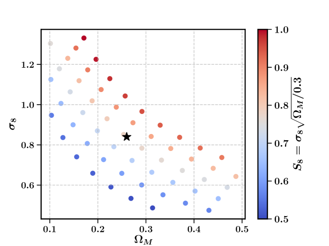
Figure 2: Distribution of the cosmologies in the $\Omega_{\mathrm{m}}-\sigma_{8}$ plane sampled with PKDGRAV3 dark-matter-only N-Body simulations. The color corresponds to the value of the $S_{8}$ parameter at each point and the star denotes the location of the fiducial cosmology. For the fiducial cosmology 50 simulations were generated, whereas 5 simulations were ran for all the other cosmologies.

3.3 Mass Map Creation

We obtain projected WL mass maps from the N-Body simulations using the UFalcon package. A detailed description of UFalcon is given in [73]. We use UFalcon to build a mass map from the discrete particle density shells of the simulations using a method developed in [74, 75, 76]. The contribution to the mass map by a single source at redshift $z_{s}$ is calculated as

$$\kappa(\hat{n})=\frac{3\Omega_{\mathrm{m}}}{2}\int_{0}^{z_{s}}\frac{dz}{E(z)a(z)}\frac{\mathcal{D}(0,z)\mathcal{D}(z,z_{s})}{\mathcal{D}(0,z_{s})}\delta\left(\frac{\mathrm{c}}{\mathrm{H}_{0}}\mathcal{D}(0,z)\thinspace\hat{n},z\right),$$ (3.4)

where $\delta$ denotes the density contrast at redshift $z$ projected onto the sphere along the line-of-sight $\hat{n}$. We introduced the dimensionless comoving distance $\mathcal{D}(z_{1},z_{2})$ between two redshifts $z_{1}$ and $z_{2}$. The function $E(z)$ is defined as

$$d\mathcal{D}=\frac{dz}{E(z)}.$$ (3.5)

Note that UFalcon avoids a full ray-tracing treatment by utilizing the Born approximation. By approximating the integral in Equation 3.4 as a discrete sum over shells of finite thickness in redshift space one can write

$$\kappa(\hat{n})\approx\frac{3\Omega_{\mathrm{m}}}{2}\sum_{b}W_{\mathrm{b}}\int_{\Delta_{z_{\mathrm{b}}}}\frac{dz}{E(z)}\delta\left(\frac{\mathrm{c}}{\mathrm{H}_{0}}\mathcal{D}(z)\thinspace\hat{n},z\right),$$ (3.6)

where the weighted contribution $W_{\mathrm{b}}$ of each shell is given by

$$W_{\mathrm{b}}=\frac{\int_{\Delta_{z_{\mathrm{b}}}}\frac{dz}{E(z)a(z)}\frac{\mathcal{D}(0,z)\mathcal{D}(z,z_{\mathrm{s}})}{\mathcal{D}(0,z_{\mathrm{s}})}}{\left(\int_{\Delta_{z_{\mathrm{b}}}}\frac{dz}{E(z)}\right)}.$$ (3.7)

To consider a continuous distribution of sources in redshift space, described by $n(z)$, the shell weights need to be modified to

$$W_{\mathrm{b}}^{n(z)}=\frac{\int_{\Delta_{z_{\mathrm{b}}}}dz\int_{z}^{z_{\mathrm{f}}}dz^{\prime}\frac{n(z^{\prime})}{a(z)E(z)}\frac{\mathcal{D}(0,z)\mathcal{D}(z,z^{\prime})}{\mathcal{D}(0,z^{\prime})}}{\left(\int_{0}^{z_{\mathrm{f}}}dz\thinspace n(z)\right)\left(\int_{\Delta_{z_{\mathrm{b}}}}\frac{dz}{E(z)}\right)},$$ (3.8)

where $z_{\mathrm{f}}=3.0$ in our setup. By pixelizing the sphere into $N_{\mathrm{pix}}$ pixels of equal area and using that the density contrast $\delta$ can be related to the pixel-averaged particle density $n_{\mathrm{p}}(\hat{n}_{\mathrm{pix}},z)$ at redshift $z$, measured within the pixel in direction $\hat{n}_{\mathrm{pix}}$, one can write down a pixelized version of the projected density contrast $\delta\left(\frac{\mathrm{\mathrm{c}}}{\mathrm{H}_{0}}\mathcal{D}(z)\thinspace\hat{n},z\right)$ as

$$\delta\left(\frac{\mathrm{c}}{\mathrm{H}_{0}}\mathcal{D}(z)\thinspace\hat{n}_{\mathrm{pix}},z\right)=\left(\frac{\mathrm{H}_{0}}{c}\right)^{3}\frac{V_{\mathrm{sim}}N_{\mathrm{pix}}}{4\pi N_{\mathrm{part}}}\frac{n_{\mathrm{p}}(\hat{n}_{\mathrm{pix}},z)}{\mathcal{D}^{2}(0,z)},$$ (3.9)

as outlined in [73]. In our work, we adapt $(900\thinspace\mathrm{Mpc}/h)^{3}$ for the simulation volume $V_{\mathrm{sim}}$ and $768^{3}$ for the number of simulated particles $N_{\mathrm{part}}$. To pixelize the sphere, the HEALPIX package [77] is used with a pixel resolution of $\texttt{NSIDE}=1024$ leading to $N_{\mathrm{pix}}=12\cdot\texttt{NSIDE}^{2}$. Please refer to [73] for a more detailed description of this procedure.

The mass maps created from the N-Body simulations using UFalcon span the full sky, containing the cosmological signal only. To produce mass maps with the same survey properties as the mock, we need to cut out patches from the simulated full-sky mass maps that have the same shape and size as the mask of the mock survey. To do so, we rotate the galaxy positions on the sky, which allows us to produce 8 simulated surveys from a single PKDGRAV3 simulation. We checked that the rotation does not introduce any artifacts, by comparing the angular power spectra of the masks of the rotated surveys. The distribution of the 8 survey masks on the sky is shown in Figure 3.

At this point, the mass maps only contain the cosmological signal. We need to add a noise component to optimally reconstruct the survey properties of the mock survey . To do so we first convert the simulated mass map $\kappa_{\mathrm{sim}}$ to a shear field $\gamma_{\mathrm{sim}}$, using the spherical Kaiser-Squires mass-mapping method (see Equation 2.3). The noise signal is drawn from the mock survey by randomly rotating the ellipticities of the galaxies in place (according to Equation 3.2) and added to the cosmological shear signal $\gamma_{\mathrm{sim}}$ on the pixel level according to

$$\gamma_{\mathrm{pix}}=\gamma_{\mathrm{noise}}+\gamma_{\mathrm{sim}}=\frac{1}{N}\sum_{j=1}^{N}\gamma_{j,\mathrm{mock}}\exp(i\phi_{j})+\gamma_{\mathrm{sim}},$$ (3.10)

with the sum running over all $N$ galaxies in the mock survey that are located in the corresponding pixel. The angles $\phi_{j}$ are drawn uniformly from the interval $[0,2\pi[$. We repeat this procedure 10 times for each PKDGRAV3 simulation, which provides us with $8\cdot 10=80$ realizations per simulation. Lastly, we convert the shear field back to a mass map, using the spherical Kaiser-Squires mass-mapping method once again.

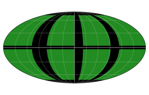
Figure 3: The 8 survey masks of the rotated mock surveys. Each one of the 8 rotated surveys spans an angular area of 5000 deg².

3.4 Cosmological Parameter Inference

We infer the constraining power in the $\Omega_{\mathrm{m}}-\sigma_{8}$ plane of the studied statistics on the basis of a stage-3-like WL survey. The measurement data-vector $\vec{X}$ is drawn from the simulations at the fiducial cosmology setting. As suggested by [49], we calculate the Figure-of-Merit (FoM) according to Equation 5.1 for all our fiducial realizations $\vec{X}_{\mathrm{i}}$ of the data-vector and we choose the realization which yields the FoM closest to the mean of the distribution of the FoMs as the measurement $\vec{X}$.

We asses the constraining power in the $\Omega_{\mathrm{m}}-\sigma_{8}$ plane for the different statistics using Bayesian inference and under the assumption that the data-vector $\vec{X}$ is drawn from a multivariate Gaussian distribution, characterized by a mean data-vector $\vec{X}_{\mathrm{M}}$ and a covariance matrix $\Sigma$. We estimate the covariance matrix $\Sigma$ from the simulated data-vectors $\vec{X}_{\mathrm{i}}$ at the fiducial cosmology as

$$\hat{\Sigma}=\frac{1}{N_{\mathrm{f}}-1}\sum_{i=1}^{N_{\mathrm{f}}}(\vec{X}_{\mathrm{i}}-\hat{\vec{X}}_{\mathrm{M}})(\vec{X}_{\mathrm{i}}-\hat{\vec{X}}_{\mathrm{M}})^{T},$$ (3.11)

where $\hat{\vec{X}}_{\mathrm{M}}$ denotes the estimate of the mean data-vector $\vec{X}_{\mathrm{M}}$ at the fiducial cosmology and $N_{\mathrm{f}}=4000$ the number of fiducial realizations.

Since we do not analytically predict the covariance matrix, nor the data-vectors, but we estimate them from simulations, the likelihood is not most accurately modelled by a Gaussian likelihood. As pointed out by [78], the use of an estimated covariance matrix requires a modification of the likelihood in order to stay unbiased. The estimation of the data-vectors from a finite number of simulations instead of using an exact prediction requires a further correction, that takes into account the additional variance [79]. Our final likelihood reads

$$L(\vec{X}|\Omega_{\mathrm{m}},\sigma_{8})\propto\left(1+\frac{N_{\mathrm{g}}}{(N_{\mathrm{g}}+1)(N_{\mathrm{f}}-1)}(\vec{X}-\hat{\vec{X}}_{\Omega_{\mathrm{m}},\sigma_{8}})^{T}\hat{\Sigma}^{-1}(\vec{X}-\hat{\vec{X}}_{\Omega_{\mathrm{m}},\sigma_{8}})\right)^{-N_{\mathrm{f}}/2},$$ (3.12)

where $N_{\mathrm{g}}=400$ indicates the number of realizations used to estimate the data vector $\hat{\vec{X}}_{\Omega_{\mathrm{m}},\sigma_{8}}$ at the cosmology in question and $N_{\mathrm{f}}=4000$ denotes the number of realizations used to estimate the covariance matrix $\Sigma$ at the fiducial cosmology.

We use the Markov Chain Monte Carlo (MCMC) ensemble sampler emcee [80] to efficiently sample the parameter space. We use flat priors ranging from 0.1 to 0.5 for $\Omega_{\mathrm{m}}$ and from 0.3 to 1.4 for $\sigma_{8}$. We use the scipy.interpolate.SmoothBivariateSpline interpolator [81], to evaluate the likelihood function at cosmologies that are not on the grid of simulated cosmologies. Each element of the data-vector is interpolated individually. We have confirmed, that the interpolator succeeds in recovering the data-vectors at cosmologies that are not on the sampled grid with the necessary precision that we require in our analysis (see Section A).

3.5 Data-Vector Compression

The evaluation of the likelihood requires the inversion of the covariance matrix. In some of our setups, especially when investigating combinations of different statistics, the concatenation of the data-vectors for different scales, tomographic bins and statistics can lead to long data-vectors and large covariance matrices. The inversion of such large matrices can be numerically unstable. In addition, we found that many of the elements of the data vectors are highly correlated. Therefore, we used a singular value decomposition (SVD) to reduce the dimensionality, along with the correlations, using the numpy.linalg.svd routine [82]. The dimensionality of the resulting data-vectors was not fixed to a pre-decided value, but was chosen for each combination of statistics individually by keeping as many SVD components as necessary to capture 99.99999% of the variance of the different realizations of the data-vector.

3.6 Systematics

One of the challenges in cosmic shear studies are systematic effects. We decided to include the three dominant effects affecting WL into our analysis, namely; galaxy intrinsic alignment (IA), multiplicative shear bias (m) and photometric redshift error ($\Delta_{z}$). In the following, we describe these systematics and how they were considered in the analysis in more detail.

Galaxy intrinsic Alignment

One of the main assumptions in WL studies is that the intrinsic ellipticities of the source galaxies are uncorrelated. It is known that this assumption does not hold true in real data due to the intrinsic correlation of the ellipticities of the galaxies with the large-scale structure and with each other. This effect is referred to as galaxy intrinsic alignment (IA) and can lead to biases in the inferred values of the cosmological parameters [21]. IA can be broken down into two different components; intrinsic-intrinsic (II) and gravitational-intrinsic (GI) alignment. The II component describes the correlations between galaxy ellipticities and the large-scale structure and the GI term refers to the correlations between the ellipticities of foreground and the sheared background galaxies in a particular region of the sky [21].

The effect of IA cannot be easily modelled with N-Body simulations. Instead, we use an approach developed by [83, 41, 84] based on the non-linear intrinsic alignment model (NLA) to calculate an IA-signal, that can be treated as an additive component to the cosmological signal as

$$\kappa_{\mathrm{tot}}=\kappa+A_{\mathrm{IA}}\thinspace\kappa_{A_{\mathrm{IA}}=1},\\$$ (3.13)

with $A_{\mathrm{IA}}$ denoting the galaxy intrinsic alignment amplitude introduced below. The IA-signal $\kappa_{A_{\mathrm{IA}}}$ can be obtained from the particle shells of the simulations in a similar fashion as the cosmological convergence signal $\kappa$ itself. To do so, the same procedure as used in UFalcon is utilized, but the weights $W_{\mathrm{b}}^{n(z)}$, given in Equation 3.8, are adapted to describe the IA-signal instead of the lensing signal

$$W_{\mathrm{b},\mathrm{IA}}^{n(z)}(A_{\mathrm{IA}})=\frac{2}{3\Omega_{\mathrm{m}}}\frac{\int_{\Delta_{z_{\mathrm{b}}}}dzF(z,A_{\mathrm{IA}})\thinspace n(z)}{\left(\int_{\Delta_{z_{\mathrm{b}}}}\frac{dz}{E(z)}\right)\left(\int_{0}^{z_{\mathrm{f}}}dz\thinspace n(z)\right)},$$ (3.14)

where $F(z,A_{\mathrm{IA}})$ is given by

$$F(z,A_{\mathrm{IA}})=-A_{\mathrm{IA}}C_{1}\rho_{\mathrm{crit}}\frac{\Omega_{\mathrm{m}}}{D_{+}(z)}\left(\frac{1+z}{1+z_{0}}\right)^{\eta}\left(\frac{\bar{L}}{L_{0}}\right)^{\beta},$$ (3.15)

with $C_{1}=5\cdot 10^{-14}h^{-2}M_{\odot}^{-1}\mathrm{Mpc}^{3}$ being a normalization constant, $D_{+}(z)$ denoting the normalized, linear growth factor and $\rho_{\mathrm{crit}}$ the critical energy density of the Universe today. The parameters $\eta$ and $\beta$ allow to model the redshift and luminosity dependence, while $A_{\mathrm{IA}}$ takes the role of an amplitude describing the overall strength of the effect. The redshift and luminosity dependence is modelled around the arbitrary pivot parameters $z_{0}$ and $L_{0}$. $\bar{L}$ denotes the average luminosity of the source galaxy population. As in [72] and [85], we do not consider the redshift and luminosity dependence, which corresponds to fixing $\eta=\beta=0$. We leave $A_{\mathrm{IA}}$ as a free parameter, that we constrain in our analysis, using a flat prior ranging from -5 to 5 for $A_{\mathrm{IA}}$, as in T18.

Multiplicative shear bias

Multiplicative shear bias (m) is another systematic effect that is expected to potentially bias the inferred values of the cosmological parameters. It can originate from multiple sources in the data reduction process, such as noise bias (see e.g. [86]), model bias (see e.g. [87]) or imperfect PSF corrections (see e.g. [88]). We incorporate the effect of multiplicative shear bias in our convergence signal by modifying the overall scale of the fluctuations as

$$\kappa_{m}=(1+m)\kappa_{m=0}.$$ (3.16)

We keep m as a nuisance parameter in our analysis and infer its value along with cosmology. We use a normal prior centered at 0.0 with a standard deviation of 0.02. The scale of the prior was chosen based on T18, assuming an improvement of $\approx 20\%$ for a stage 3 WL survey. In the tomographic setup, we adapt one multiplicative shear bias parameter $\mathrm{m}_{\mathrm{i}}$ for each tomographic bin.

Photometric redshift error

Since WL surveys need to target a large number of galaxies, it is not feasible to determine their redshift spectroscopically but only photometrically. This can lead to a biased redshift distribution of the source galaxy population. As shown in previous studies, such as [89], errors in the redshift distribution can bias the inferred values of cosmological parameters. We take this effect into account by introducing the nuisance parameter $\Delta_{z}$, which describes a global shift of the redshift distribution $n(z)$ as

$$n^{\prime}(z)=n(z-\Delta_{z}),$$ (3.17)

where $n^{\prime}(z)$ denotes the shifted redshift distribution of the source galaxies. We infer the value of $\Delta_{z}$ in our analysis, using a normal prior centered at 0.0 with a standard deviation of 0.015, which is motivated based on the priors used in T18 and assuming an $\approx 20\%$ improvement for a stage 3 WL survey. In the tomographic setup we use one parameter $\Delta_{z,\mathrm{i}}$ for each tomographic bin.

Systematics emulator

Including the nuisance parameters, we require to sample a 5 (or 11 for a tomographic setup) dimensional parameter space in the MCMC procedure. In order to make accurate predictions with the interpolator described in Section 3.4, a sufficiently dense sampling of the parameter space is needed. This requires us to run simulations for a number of parameter configurations that is exponentially increasing with the dimension of the sampled hypercube. We use an emulator approach to reduce the number of required simulations.
The idea is to only simulate a sub-sample of the full simulation grid and use these simulations to fit a parametric model for each element of the data-vector, emulating the effect of the systematics on the statistics level directly as

$$\vec{d}(\Omega_{\mathrm{m}},\sigma_{8},A_{\mathrm{IA}},m,\Delta_{z}) =\sum_{i}d_{i}(\Omega_{\mathrm{m}},\sigma_{8},A_{\mathrm{IA}},m,\Delta_{z})\hat{\vec{e}}_{i}$$

$$=\sum_{i}a^{i}(\Omega_{\mathrm{m}},\sigma_{8},A_{\mathrm{IA}},m,\Delta_{z})\cdot d_{i}(\Omega_{\mathrm{m}},\sigma_{8})\hat{\vec{e}}_{i},$$ (3.18)

where $d_{i}(\Omega_{\mathrm{m}},\sigma_{8})$ denotes the value of the $i$th element of the systematics-free data-vector as obtained by using the interpolator described in Section 3.4 and $a^{i}(\Omega_{\mathrm{m}},\sigma_{8},A_{\mathrm{IA}},m,\Delta_{z})$ the parametric scale factor, which modifies the interpolated data-vector element to emulate the effect of the systematics. We note, that the separation in Equation 3.18 is not physically motivated in general. We checked that this approach does not introduce significant biases in our results (see Section B). Following the Occam’s razor, we started with a simplistic model for $a^{i}(\Omega_{\mathrm{m}},\sigma_{8},A_{\mathrm{IA}},m,\Delta_{z})$ and continuously increased its complexity until the accuracy of the predictions fulfilled our requirements, ending up with a model containing 16 parameters that we fit individually for each element of the data vector. We describe the emulator as well as the tests that we performed on it, in more detail in Section B.

3.7 Codebase

To allow the reader to reproduce and further understand the methodology of this work, we publish the repository NGSF, containing the pipeline used to run the analysis. In addition to the main pipeline, we developed three independent packages as part of this project that are used in the analysis. We made an effort to organize our codebase in a user-friendly manner, in order to simplify running such analyses in the future and to make them more accessible and easily extendable. In particular, we tried to make it easy to implement user-specific, map-based WL statistics, that can be used in estats and the NGSF pipeline. The developed packages are estats, esub-epipe and ekit. All packages are also publicly available on the Python package index PyPi . The links to the source code and the documentation pages of the packages can be found in the NGSF repository. The estats package contains the major building blocks of the pipeline. The usage of the different estats modules in this analysis is illustrated in Figure 4.

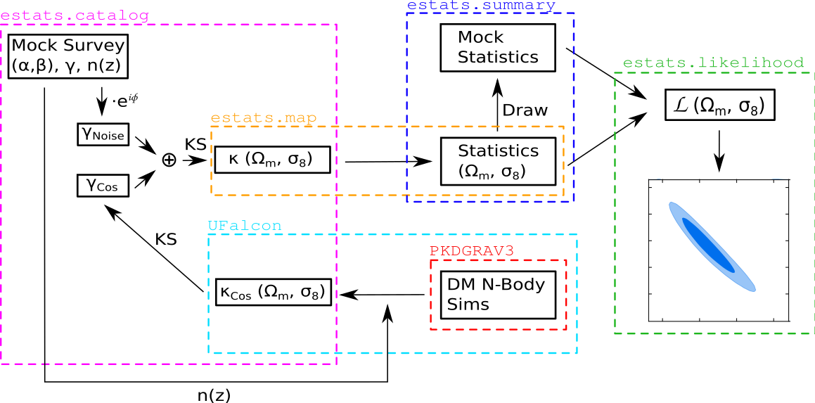
Figure 4: A schematic illustration of the analysis performed in this work. We indicate which parts of the code, described in Section 3.7, are used in which steps of the analysis using the dashed boxes. The label KS indicates where the Kaiser-Squires map making procedure was used. The details of the steps are described in detail in Section 3.

4 Simulated non-tomographic Statistics

We present our findings for the cosmology dependence of the studied non-tomographic statistics; i.e. we study their dependency on the $S_{8}$ parameter in Figure 5. The colored curves in each panel of Figure 5 show how the statistics change with $S_{8}$. The black data points are centered at the fiducial cosmology, with the error bars indicating the measurement error expected for a stage-3-like WL survey. The error bars are estimated from the realizations of the statistics at the fiducial cosmology. For brevity, we decided to only present the results for one of the 9 considered scales, for the non-Gaussian statistics (see Section 4.2). We further present the correlation matrix for the non-tomographic combination of all studied statistics, namely CLs+PC+MC+MFs, in Figure 6. We refrain from showing the results for the tomographic statistics, since we believe that their presentation does not provide any additional insights to the reader. However, we do present the cosmological constraints, that we find in the non-tomographic, as well as the tomographic setup, in Section 5. We also summarize and explain the configuration choices, that we made for the different statistics and their most important features in this section.

4.1 Angular Power Spectrum (CLs)

The angular power spectrum (CLs) is calculated directly from the simulated mass maps using the anafast routine implemented in healpy [77] without performing any prior smoothing of the maps. Each pixel is weighted by the number of galaxies that fall into its regime. We consider an angular mutlipole range from $\ell=100$ to $\ell=1000$ using 20 linearly spaced bins. The number of bins was chosen, such that a further division into more bins does not increase the constraining power any further. The lower limit of the multipole range ($\ell=100$) was chosen in order to avoid large-scale regimes, where relativistic corrections become significant [42]. We note that PKDGRAV3 actually includes relativistic corrections and would therefore be suitable to include scales larger than $\ell=100$, but as one of the goals of this work is to demonstrate that the addition of non-Gaussian statistics allows to apply conservative scale cuts, we have decided to not include these scales. To optimally extract the non-Gaussian features of the maps, we apply a set of smoothing kernels to the maps in order to select features of different sizes. We found, that when applying a Gaussian smoothing kernel with a full-width-at-half-maximum (FWHM) of 10.5 arcmin, which corresponds to the smallest scale considered for the non-Gaussian statistics (see Section 4.2), the measured CLs drop to $\approx 20\%$ compared to the CLs extracted from the unsmoothed maps at a multipole of $\ell\approx 1000$. Hence, we chose $\ell=1000$ as the upper limit for the multipole range, in order to make the constraints obtained from the CLs more comparable to the ones from the non-Gaussian statistics. The dependency of the non-tomographic CLs on $S_{8}$ is shown in the right, bottom panel of Figure 5. In the tomographic setup, we additionally include the cross-power-spectra between the 4 tomographic bins in the inference process. Note that the CLs measured in this analysis are not corrected for masking effects and therefore should not be compared directly to the CLs predicted analytically from a theory code, as these predictions are typically done for a full-sky map. The parameter constraints in this work are not biased due to the missing correction for masking effects, since the predictions for the CLs at different cosmologies are extracted from the simulations using the same survey mask as it is used for the mock measurement. The contribution from the survey noise (indicated by the black, dashed line in Figure 5) increases on small scales and therefore we obtain the most cosmological constraining power from the data bins at large scales, below $\ell\approx 500$. We can learn from Figure 6 that the different data bins of the CLs are highly correlated.

4.2 Peak and Minimum Counts (PC/MC)

For the non-Gaussian statistics we adapt a multiscale scheme as it was previously done by [49]. Each mass map is smoothed using 9 different Gaussian smoothing kernels with a FWHM of [31.6, 29.0, 26.4, 23.7, 21.1, 18.5, 15.8, 13.2, 10.5] arcmin, respectively. The statistics are then calculated from each smoothed version of the mass map. The total data-vector for each statistic is obtained by concatenation of the 9 single scale data-vectors. The application of different smoothing kernels to the mass maps allows the selection of map features of different sizes. It was shown, in [49], that the consideration of even smaller scales leads to a further increase of the constraining power. However, on scales smaller than $\approx$ 8 arcmin baryonic effects cannot be neglected for the PC [90]. Hence, we decided to consider only scales larger than 10 arcmin for all non-Gaussian statistics.

The application of a smoothing kernel to the mass maps washes out the small-scale fluctuations of the maps and therefore changes the significant range of $\kappa$ for the PC/MC. Hence, we adapted the range of $\kappa$ used to record peaks and minima on the mass maps depending on the applied smoothing kernel, to optimally resolve the distribution of the peaks and minima on all scales. This complex binning scheme could be avoided by binning the map features in bins of signal-to-noise ratio (SNR) instead of $\kappa$, as it is was mostly done in previous studies. However, we found that by doing so the cosmological constraining power of the PC/MC is diminished. Recording the map features as a function of SNR instead of $\kappa$, requires to rescale the $\kappa$ values of the extracted features by the mean standard deviation $<\sigma_{\kappa}>$ of the mass map, estimated on a pixel level (since the SNR is defined by SNR = $\kappa/<\sigma_{\kappa}>$). As $<\sigma_{\kappa}>$ itself carries a strong dependency on cosmology, the PC/MC become more self-similar and cosmological information is lost. In the case of a combined analysis, using PC/MC and CLs, the lost constraining power is regained since the cosmology dependence of $<\sigma_{\kappa}>$ is captured by the CLs. In total we use 15 equally spaced bins per scale. This number has been chosen, such that increasing the number of bins does not improve the cosmological constraints anymore. To suppress the shot noise contribution, we chose the edges of the outermost bins, such that for each cosmological setup at least 30 peaks/minima are registered in each bin. The remaining $\kappa$ range is divided into equally spaced bins. We present the simulated PC/MC for a selected smoothing scale of FWHM=21.1 arcmin in the top row of Figure 5. The most information about $S_{8}$ is obtained from the highest/lowest $\kappa$ bins of the PC/MC, respectively. The reason being, that such features of the map are generated by very dense halos and very under-dense voids, respectively and it is unlikely that such events are produced by random noise. While the number of less extreme features, as they are recorded in the other data bins, is certainly larger, the noise contribution (indicated by the black, dashed line) is dominating in this regime, suppressing the cosmological signal. With the increase in galaxy density in future surveys, the contribution from these data bins is expected to grow. From the correlation matrix in Figure 6, we find that there is some correlation present between the map features found on different scales for both the PC and MC. This is not unexpected, as the applied smoothing scales do not differ enough to wash out the features registered on other scales completely. We find that there is some correlation between the PC/MC and the CLs, indicating that they partly record similar information of the mass maps.

4.3 Minkowski Functionals (MFs)

We use 16 different excursion sets $Q_{t}$, spaced linearly in SNR from -2 to +2 for each scale. We chose the number of considered excursion sets such that including more does not lead to an increase in the constraining power. The thresholds $t$ of the sets are chosen in terms of the signal-to-noise ratio (SNR), i.e. the set $Q_{t}$ contains only pixels with values $\kappa\geq\nu\cdot<\sigma_{\kappa}>$, where the average standard deviation of the mass map $<\sigma_{\kappa}>$ is estimated on a pixel level. As for the PC/MC, we present the MFs for only one selected scale, namely FWHM=21.1 arcmin, in Figure 5. In contrast to the other statistics, we do not show the noise contribution for the MFs, since the noise cannot be understood as an additive component on the statistics level, as it is the case for the CLs (and approximately for the PC/MC). Contrarily to the PC/MC we find less correlation between the MFs and the CLs, indicating that the MFs probe a different kind of information than the CLs, PC and MC (see Figure 6).

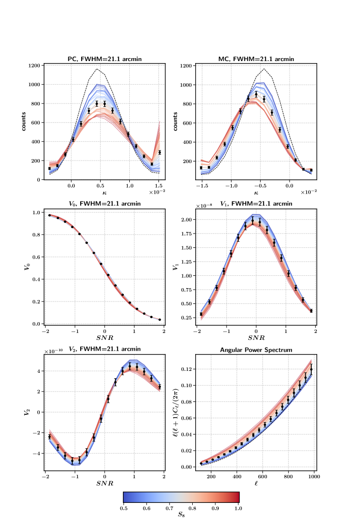
Figure 5: The simulated statistics recorded in a non-tomographic setup for varying $S_{8}$. The two panels at the top illustrate the $S_{8}$ dependency of the peak counts (PC) and minimum counts (MC), binned as a function of the convergence value $\kappa$ of the detected peaks/minima. The second row and the left, bottom panel show the simulated Minkowski functionals (MFs), binned as a function of signal-to-noise ratio (SNR). For brevity, we decided to only show the results for one selected scale for the non-Gaussian statistics, namely FWHM=21.1 arcmin. In the bottom, right panel the angular power spectrum (CLs) is presented. The black data points shown in each panel are centered at the fiducial cosmology. The error bars indicate the errors estimated for a stage-3-like WL survey. For the statistics for which the noise contribution can be understood as an (approximately) additive component to the cosmological signal, it is indicated by the black, dashed line.

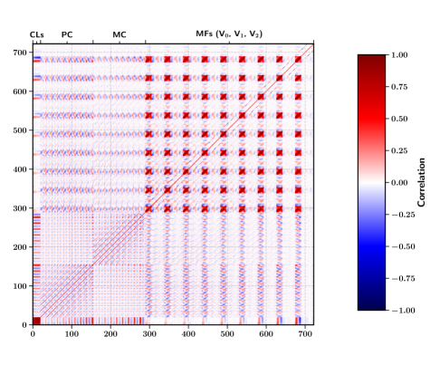
Figure 6: The full non-tomographic correlation matrix at the fiducial cosmology, including all studied statistics, before applying the singular value decomposition. The statistics are ordered from left to right as Angular Power Spectrum (CLs), peak counts (PC), minimum counts (MC) and Minkowski functionals (MFs) (in order V₀, V₁ and V₂). For the PC, MC and MFs all 9 scales are concatenated from largest to smallest.

5 Cosmological Constraints

We compare the constraints in the $\Omega_{\mathrm{m}}-\sigma_{8}$ and $A_{\mathrm{IA}}-S_{8}$ plane for the different statistics. We summarize our findings in Table 1 and Table 2, where we present the constraints on $\Omega_{\mathrm{m}}$, $\sigma_{8}$, $S_{8}$ and $A_{\mathrm{IA}}$ for all statistics and we note the FoM (Figure-of-Merit) in the $\Omega_{\mathrm{m}}-\sigma_{8}$ plane, computed as

$$\mathrm{FoM}=\frac{1}{\sqrt{|\hat{\Sigma}(\Omega_{\mathrm{m}},\sigma_{8})|}},$$ (5.1)

according to T18. The covariance matrix $\hat{\Sigma}$ is estimated from the MCMC chains. The FoM is anti-proportional to the area of the constraints in the $\Omega_{\mathrm{m}}-\sigma_{8}$ plane, with a larger value of the FoM indicating stronger constraints on $\Omega_{\mathrm{m}}$ and $\sigma_{8}$.

As a reference, we compare our constraints to the results found by the Planck 2018 survey [9] and the DES cosmic shear analysis from the Year 1 data sample [T18]. We note that a direct comparison of the constraints found in this work with the results found by T18 is not straightforward, as we have made some different design choices in our analysis. The main differences include; 1. We use the angular power spectrum, whereas T18 uses 2-point real space correlators, 2. We do not infer the redshift dependence of galaxy intrinsic alignment, 3. We use more conservative scale cuts in our analysis ($\ell\in[100,1000]$ as opposed to $\theta\in[2.5,250]$ arcmin in T18). Given these differences, we suggest the reader to consider the results found by T18 as a reference for the scale of our constraints only.

All presented constraints were obtained using an MCMC sampling routine of the parameter space, running 30 chains with an individual length of 50’000 samples.

5.1 Non-tomographic Constraints

The non-tomographic constraints in the $\Omega_{\mathrm{m}}-\sigma_{8}$ plane are shown in Figure 7. We recover the typical $\Omega_{\mathrm{m}}-\sigma_{8}$ degeneracy for the CL analysis (red contour, upper left panel in Figure 7). For the non-Gaussian statistics, a similar degeneracy is found, although it is weaker when compared to the CLs. This also reflects itself in the FoM (see Table 1), yielding a relative improvement by a factor of $\approx$11, $\approx$3 and $\approx$5 over the CL analysis, for the PC, MC and MFs, respectively. While for the PC and MC, the direction of the degeneracy is only slightly different as for the CLs, we record a different degeneracy direction for the MFs, indicating that the MFs might help to break the degeneracy of the other statistics in a combined setup (see Section 5.3 below). Overall, we find that all non-Gaussian statistics are less affected by the $\Omega_{\mathrm{m}}-\sigma_{8}$ degeneracy and yield stronger constraints than the CL analysis in a non-tomographic setup and without the consideration of systematic effects.

None of the statistics considered is able to put constraints on multiplicative shear bias, nor photometric redshift error, leading to the constraints on $m$ and $\Delta_{z}$ being prior dominated for all studied statistics. The uncertainty on $m$ and $\Delta_{z}$ contributes to the broadening of the contours in the $S_{8}$ direction, as seen in Figure 7 (blue contours). However, the major contribution to the broadening in $S_{8}$ direction originates from the degeneracy with the galaxy intrinsic alignment amplitude $A_{\mathrm{IA}}$. All statistics suffer from a loss of constraining power when systematic effects are included, yielding a deterioration of the FoM by a factor of $\approx$3, $\approx$3, $\approx$1.8 and $\approx$1.8 for the CLs, PC, MC and MFs, respectively. We further discuss the non-tomographic constraints on galaxy intrinsic alignment in Section 5.4 below.

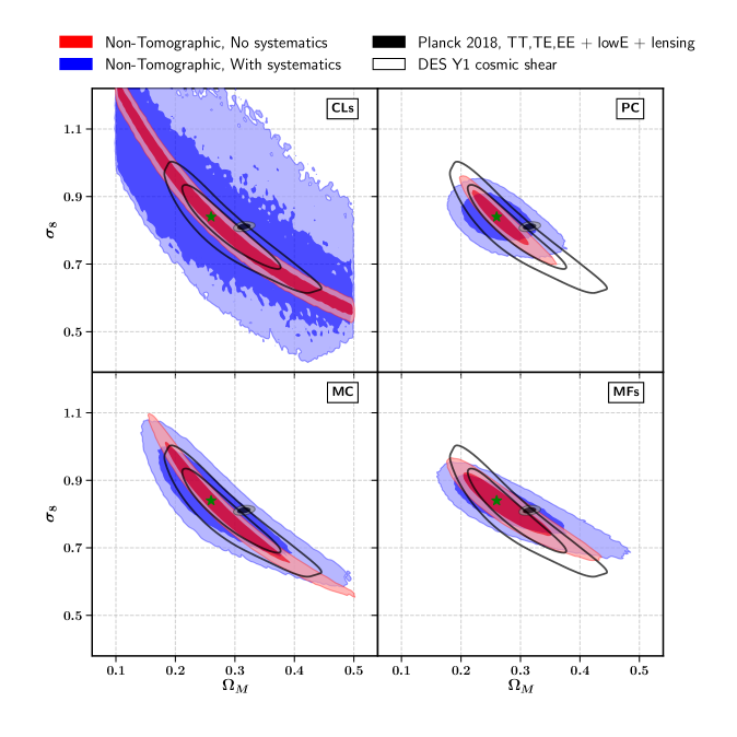
Figure 7: Constraints in the $\Omega_{\mathrm{m}}-\sigma_{8}$ plane found in the non-tomographic setup. While we have fixed the nuisance parameters to $A_{\mathrm{IA}}=0,m=0,\Delta_{z}=0$, when obtaining the red contours, we find the blue contours when inferring the values of the nuisance parameters simultaneously with the cosmological parameters. For reference, we have added the contours found by the Planck 2018 [9] and DES Y1 cosmic shear [66] surveys. Note that since we drew the mock measurement in this study from the fiducial simulations, the contours are centered at the fiducial cosmology, indicated by the green star. Therefore, the location of our contours should not be compared to the location of the contours found by DES Y1 and Planck 2018. Only their relative sizes should be compared. All contours show the 68% and 95 % percentiles of the marginalized 2D-distributions.

5.2 Tomographic Constraints

Since tomography is known to help to improve the robustness of the CL analysis to galaxy intrinsic alignment, we further study how much the statistics profit from a tomographic setup. We present the tomographic constraints in Figure 8. While we find that tomography increases the constraining power of all studied statistics, there is a large difference in the improvement between the CLs and the non-Gaussian statistics, with the non-Gaussian statistics profiting less (see Table 1). From a comparison of the FoM between the non-tomographic and tomographic setups (without the consideration of systematics), we find a relative increase of the FoM, upon introducing tomography, by a factor of $\approx$4, $\approx$1.2, $\approx$2, $\approx$1.1 for the CLs, PC, MC and MFs, respectively. One possible reason for this difference is the fact that the non-Gaussian statistics are specifically designed to pick up the features of the projected matter field. Those features become more prominent as one integrates further over the matter field and sums up the lensing effects from structures along the line of sight. Therefore, an integration over a larger redshift range leads to more pronounced over/under-densities on the mass maps. We also attribute this result to the fact that we include cross-power-spectra between different tomographic bins in the CL analysis, while we do not consider such cross-correlations for the non-Gaussian statistics.

While tomography can increase the cosmological constraining power by providing more information about the three-dimensional structure of the matter field, its main impact is to constrain galaxy intrinsic alignment, leading to a more pronounced gain in constraining power over the non-tomographic setup when systematic effects are taken into account. Again, the CLs profit the most from tomography with a relative increase of the FoM by a factor of $\approx$10, while the non-Gaussian statistics gain by a factor of $\approx$3.4, $\approx$3.8 and $\approx$2 for the PC, MC and MFs, respectively (see magenta contours in Figure 8). Although the non-Gaussian statistics do not profit from tomography as much as the CLs do, their cosmological constraining power remains better since they can extract more cosmological information in the first place. Note that the non-Gaussian statistics achieve FoM values without tomography that are similar to those for the CL analysis with tomography (comparing the blue to the red entries in Table 1). The PC show the most potential by yielding constraints in the $\Omega_{\mathrm{m}}-\sigma_{8}$ plane that are about double in FoM compared to those for the CLs. However, we note that in the $S_{8}$ direction the constraints are broader, which is related to the slightly different direction of the degeneracy and the larger uncertainty on $A_{\mathrm{IA}}$.

We further discuss the tomographic constraints on galaxy intrinsic alignment in Section 5.4 below.

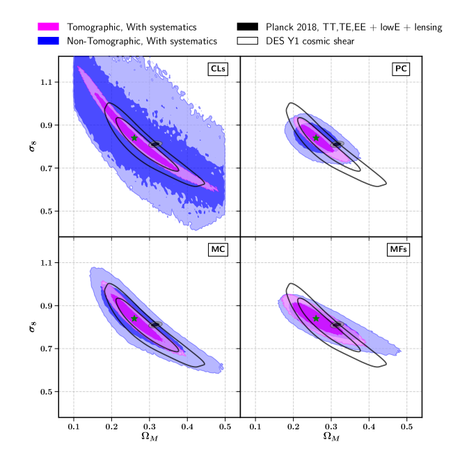
Figure 8: We compare the constraining power of the different statistics in the $\Omega_{\mathrm{m}}-\sigma_{8}$ plane when inferring cosmology and the nuisance parameters simultaneously. While we used a non-tomographic configuration to obtain the blue constraints, a tomographic setup was used to find the magenta contours. For reference, we have added the contours found by the Planck 2018 [9] and DES Y1 cosmic shear [66] surveys. Note that since we drew the mock measurement in this study from the fiducial simulations, the contours are centered at the fiducial cosmology, indicated by the green star. Therefore, the location of our contours should not be compared to the location of the contours found by DES Y1 and Planck 2018. Only their relative sizes should be compared. All contours show the 68% and 95 % percentiles of the marginalized 2D-distributions.

Table 1: A comparison of the constraints on all parameters (except for $m$ and $\Delta_{z}$), inferred using the individual statistics. The constraints are presented as the median including the 95% confidence intervals in both directions. The fiducial value for each parameter is indicated in brackets, on the first line. We also denote the ranges of the flat priors that we used in the MCMC procedure for each parameter, on the second line. The Figure-of-Merit (FoM) was calculated according to T18.

	tomo	sys	$\Omega_{\mathrm{m}}$ (0.26)	$\sigma_{8}$ (0.84)	$S_{8}$ (0.79)	FoM	$A_{\mathrm{IA}}$ (0.0)
Prior	-	-	0.1 – 0.5	0.3 – 1.4	-	-	-5 – 5
CLs	N	N	$0.29^{+0.20}_{-0.18}$	$0.83^{+0.35}_{-0.28}$	$0.760^{+0.052}_{-0.059}$	207	–
	N	Y	$0.28^{+0.20}_{-0.18}$	$0.87^{+0.39}_{-0.38}$	$0.80^{+0.33}_{-0.26}$	58	$0.2^{+4.1}_{-4.6}$
	Y	N	$0.26^{+0.13}_{-0.12}$	$0.85^{+0.22}_{-0.20}$	$0.776^{+0.027}_{-0.028}$	659	–
	Y	Y	$0.26^{+0.15}_{-0.14}$	$0.85^{+0.23}_{-0.22}$	$0.774^{+0.035}_{-0.035}$	485	$-0.01^{+0.42}_{-0.44}$
PC	N	N	$0.268^{+0.066}_{-0.060}$	$0.83^{+0.10}_{-0.11}$	$0.781^{+0.030}_{-0.031}$	1780	–
		Y	$0.265^{+0.080}_{-0.075}$	$0.831^{+0.094}_{-0.10}$	$0.777^{+0.096}_{-0.10}$	586	$-0.1^{+1.9}_{-2.2}$
	Y	N	$0.267^{+0.067}_{-0.061}$	$0.833^{+0.087}_{-0.096}$	$0.782^{+0.028}_{-0.029}$	2074	–
		Y	$0.265^{+0.060}_{-0.057}$	$0.834^{+0.079}_{-0.089}$	$0.780^{+0.033}_{-0.034}$	1964	$0.14^{+0.90}_{-0.84}$
MC	N	N	$0.28^{+0.15}_{-0.12}$	$0.81^{+0.21}_{-0.23}$	$0.774^{+0.041}_{-0.046}$	509	–
		Y	$0.28^{+0.15}_{-0.12}$	$0.82^{+0.20}_{-0.20}$	$0.773^{+0.089}_{-0.094}$	273	$-0.1^{+1.6}_{-2.0}$
	Y	N	$0.268^{+0.099}_{-0.090}$	$0.84^{+0.15}_{-0.14}$	$0.780^{+0.029}_{-0.029}$	1097	–
		Y	$0.266^{+0.092}_{-0.084}$	$0.84^{+0.14}_{-0.14}$	$0.779^{+0.036}_{-0.036}$	1031	$0.1^{+1.1}_{-1.0}$
MFs	N	N	$0.282^{+0.11}_{-0.094}$	$0.82^{+0.12}_{-0.13}$	$0.785^{+0.049}_{-0.053}$	828	–
		Y	$0.29^{+0.14}_{-0.11}$	$0.82^{+0.11}_{-0.12}$	$0.788^{+0.098}_{-0.10}$	457	$0.1^{+1.8}_{-1.9}$
	Y	N	$0.271^{+0.092}_{-0.085}$	$0.830^{+0.094}_{-0.10}$	$0.783^{+0.063}_{-0.067}$	875	–
		Y	$0.267^{+0.090}_{-0.084}$	$0.832^{+0.095}_{-0.097}$	$0.779^{+0.065}_{-0.070}$	895	$0.1^{+1.1}_{-1.0}$
Planck 2018 TT,TE,EE + lowE + lensing	–	–	$0.315^{+0.015}_{-0.014}$	$0.811^{+0.012}_{-0.012}$	$0.832^{+0.025}_{-0.025}$	23170	–
DES Y1, cosmic shear	Y	Y	$0.290^{+0.11}_{-0.094}$	$0.80^{+0.15}_{-0.16}$	$0.778^{+0.055}_{-0.057}$	578	$0.8^{+1.3}_{-1.3}$

5.3 Combined Constraints

With the non-Gaussian statistics probing a different kind of information of the mass maps than the CLs, we demonstrate that a combination of the different statistics yields stronger constraints on cosmology, than using the individual statistics alone. The constraints obtained when using different combinations of statistics are presented in Figure 9, for both the non-tomographic and tomographic setups. For comparison, we added the constraints that we find with the tomographic CL analysis (in yellow). A quantitative comparison of the constraints is presented in Table 2.

Non-tomographic Results

With the CLs and PC carrying the strongest cosmological signal, we find that combining the two yields tight constraints on the cosmological parameters in the tomographic and non-tomographic setup (CLs+PC). However, we observe that the PC capture nearly all the cosmological information that is recorded by the CLs, making the contribution of the CLs subdominant in this setup. The addition of MFs does not increase the constraining power significantly (CLs+PC+MFs) and neither do the MC (CLs+PC+MC+MFs). We note however, that a combination of CLs+MC+MFs yields a similar FoM than CLs+PC. The different direction of the $\Omega_{\mathrm{m}}-\sigma_{8}$ degeneracy of the MFs helps to tighten the constraints of the CLs and MC (CLs+MFs and CLs+MC+MFs), but when the PC are included, yielding constraints that are much smaller than the ones found with the MFs, the effect becomes negligible (CLs+PC+MC+MFs). In the described non-tomographic setup, without the consideration of systematic effects, the addition of the PC / all non-Gaussian statistics to the CLs increases the FoM by a factor of $\approx$4.1 and $\approx$4.2, respectively.

With the inclusion of systematic effects into the analysis, the contributions of the MC and MFs become more important, as they are more robust to galaxy intrinsic alignment. We find that in a non-tomographic setup, the addition of MC and MFs to the CLs and PC helps to reduce the broadening of the contours in the $S_{8}$ direction, that is caused mostly by the uncertainty on $A_{\mathrm{IA}}$ (CLs+PC+MC+MFs). As already noted for the individual non-Gaussian statistics, we find that a combination of CLs and non-Gaussian statistics yields tighter constraints in the $\Omega_{\mathrm{m}}-\sigma_{8}$ plane, without using tomography, than using the CL analysis with tomography (comparing the blue to the red entries in Table 2).

Tomographic Results

While the non-tomographic combination of all statistics yields competitive results, the addition of tomography further increases the cosmological constraining power. When neglecting systematic effects, we find the same trend as in the non-tomographic case, with the PC contributing most of the cosmological constraining power, a small contribution by the CLs and neither the MC nor the MFs contributing significantly for a combination of all statistics.

When including systematic effects we observe an increase of the FoM by a factor of $\approx$5.5 as compared to the tomographic CL analysis and by a factor of $\approx$2.3 over the non-tomographic setup when all statistics are considered. The gain is mainly achieved by the heightened constraints on $A_{\mathrm{IA}}$, thanks to the cross-spectra considered in the tomographic CL analysis. With the tomographic CLs constraining $A_{\mathrm{IA}}$, the role of the MC and MFs in the tomographic setup is negligible, as their main contribution in the non-tomographic case was to add robustness to galaxy intrinsic alignment. Again, we leave it to further studies to investigate if the inclusion of cross-correlations between different tomographic bins for the non-Gaussian statistics yields similar constraints on $A_{\mathrm{IA}}$.

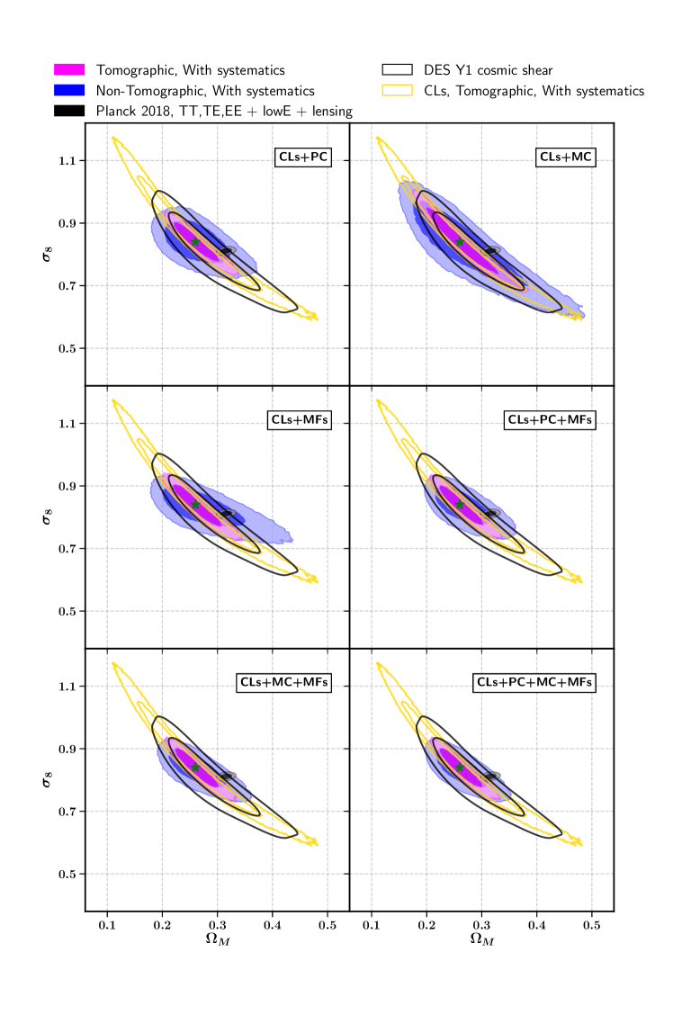
Figure 9: We compare the constraining power of different combinations of statistics in the $\Omega_{\mathrm{m}}-\sigma_{8}$ plane when inferring cosmology and nuisance parameters simultaneously. While we used a non-tomographic configuration to find the blue constraints, we find the magenta contours using a tomographic setup. For reference, we have added the contours found by the Planck 2018 [9] and DES Y1 cosmic shear [66] surveys. Note that since we drew the mock measurement in this study from the fiducial simulations, the contours are centered at the fiducial cosmology, indicated by the green star. Therefore, the location of our contours should not be compared to the location of the contours found by DES Y1 and Planck 2018. Only their relative sizes should be compared. All contours show the 68% and 95 % percentiles of the marginalized 2D-distributions.

Table 2: Same as Table 1, but comparing the parameter constraints using different combinations of the studied statistics.

	tomo	sys	$\Omega_{\mathrm{m}}$ (0.26)	$\sigma_{8}$ (0.84)	$S_{8}$ (0.79)	FoM	$A_{\mathrm{IA}}$ (0.0)
Prior	-	-	0.1 – 0.5	0.3 – 1.4	-	-	-5 – 5
CLs	Y	Y	$0.26^{+0.15}_{-0.14}$	$0.85^{+0.23}_{-0.22}$	$0.774^{+0.035}_{-0.035}$	485	$-0.01^{+0.42}_{-0.44}$
CLs + PC	N	N	$0.267^{+0.066}_{-0.060}$	$0.83^{+0.10}_{-0.11}$	$0.781^{+0.030}_{-0.031}$	1809	–
		Y	$0.265^{+0.078}_{-0.073}$	$0.835^{+0.091}_{-0.096}$	$0.780^{+0.090}_{-0.092}$	648	$0.0^{+1.8}_{-2.1}$
	Y	N	$0.265^{+0.061}_{-0.057}$	$0.835^{+0.085}_{-0.092}$	$0.781^{+0.023}_{-0.024}$	2624	–
		Y	$0.263^{+0.056}_{-0.051}$	$0.836^{+0.077}_{-0.085}$	$0.780^{+0.028}_{-0.028}$	2444	$0.02^{+0.36}_{-0.37}$
CLs + MFs	N	N	$0.272^{+0.076}_{-0.070}$	$0.827^{+0.099}_{-0.10}$	$0.782^{+0.045}_{-0.046}$	1179	–
		Y	$0.279^{+0.11}_{-0.092}$	$0.825^{+0.087}_{-0.090}$	$0.789^{+0.10}_{-0.097}$	597	$0.1^{+1.7}_{-1.9}$
	Y	N	$0.265^{+0.059}_{-0.056}$	$0.834^{+0.086}_{-0.094}$	$0.780^{+0.030}_{-0.031}$	2054	–
		Y	$0.264^{+0.059}_{-0.055}$	$0.835^{+0.085}_{-0.088}$	$0.780^{+0.032}_{-0.032}$	2040	$0.01^{+0.42}_{-0.45}$
CLs + MC	N	N	$0.28^{+0.13}_{-0.11}$	$0.81^{+0.19}_{-0.21}$	$0.774^{+0.041}_{-0.044}$	632	–
		Y	$0.28^{+0.14}_{-0.12}$	$0.82^{+0.16}_{-0.18}$	$0.772^{+0.083}_{-0.090}$	337	$-0.1^{+1.6}_{-1.9}$
	Y	N	$0.266^{+0.090}_{-0.083}$	$0.84^{+0.14}_{-0.14}$	$0.779^{+0.022}_{-0.023}$	1469	–
		Y	$0.264^{+0.087}_{-0.078}$	$0.84^{+0.13}_{-0.13}$	$0.779^{+0.028}_{-0.028}$	1363	$0.00^{+0.39}_{-0.41}$
CLs + PC + MFs	N	N	$0.267^{+0.057}_{-0.052}$	$0.830^{+0.093}_{-0.097}$	$0.780^{+0.031}_{-0.032}$	2052	–
		Y	$0.268^{+0.070}_{-0.063}$	$0.831^{+0.076}_{-0.086}$	$0.783^{+0.073}_{-0.073}$	934	$0.0^{+1.5}_{-1.6}$
	Y	N	$0.264^{+0.056}_{-0.052}$	$0.835^{+0.081}_{-0.088}$	$0.780^{+0.026}_{-0.027}$	2524	–
		Y	$0.264^{+0.054}_{-0.049}$	$0.835^{+0.078}_{-0.084}$	$0.780^{+0.028}_{-0.027}$	2513	$0.00^{+0.39}_{-0.41}$
CLs + MC + MFs	N	N	$0.268^{+0.058}_{-0.053}$	$0.829^{+0.089}_{-0.10}$	$0.780^{+0.032}_{-0.033}$	1973	–
		Y	$0.265^{+0.071}_{-0.064}$	$0.831^{+0.078}_{-0.082}$	$0.778^{+0.064}_{-0.070}$	1027	$-0.1^{+1.4}_{-1.5}$
	Y	N	$0.265^{+0.056}_{-0.052}$	$0.834^{+0.082}_{-0.088}$	$0.780^{+0.026}_{-0.027}$	2487	–
		Y	$0.264^{+0.053}_{-0.050}$	$0.835^{+0.079}_{-0.084}$	$0.780^{+0.028}_{-0.028}$	2494	$0.01^{+0.41}_{-0.43}$
CLs + PC + MC + MFs	N	N	$0.267^{+0.056}_{-0.051}$	$0.830^{+0.092}_{-0.096}$	$0.780^{+0.030}_{-0.031}$	2199	–
		Y	$0.265^{+0.064}_{-0.059}$	$0.831^{+0.075}_{-0.086}$	$0.778^{+0.061}_{-0.065}$	1113	$0.0^{+1.2}_{-1.4}$
	Y	N	$0.264^{+0.054}_{-0.050}$	$0.835^{+0.078}_{-0.084}$	$0.781^{+0.025}_{-0.025}$	2695	–
		Y	$0.263^{+0.052}_{-0.049}$	$0.836^{+0.077}_{-0.083}$	$0.780^{+0.028}_{-0.027}$	2576	$0.01^{+0.40}_{-0.41}$
Planck 2018 TT,TE,EE + lowE + lensing	–	–	$0.315^{+0.015}_{-0.014}$	$0.811^{+0.012}_{-0.012}$	$0.832^{+0.025}_{-0.025}$	23170	–
DES Y1, cosmic shear	Y	Y	$0.290^{+0.11}_{-0.094}$	$0.80^{+0.15}_{-0.16}$	$0.778^{+0.055}_{-0.057}$	578	$0.8^{+1.3}_{-1.3}$

5.4 Constraints on Galaxy intrinsic Alignment

Figure 10 shows the constraints in the $A_{\mathrm{IA}}-S_{8}$ plane for the individual statistics, as well as for the combination of CLs and MC (CLs+PC) and all statistics (CLs+PC+MC+MFs).

The CLs are unable to constrain $A_{\mathrm{IA}}$ in the non-tomographic case and their cosmological constraining power is strongly diminished when $A_{\mathrm{IA}}$ is included in the analysis. This is due to the broadening of the contours in the $S_{8}$ direction, caused by the pronounced degeneracy between $S_{8}$ and $A_{\mathrm{IA}}$ (top, left panel in Figure 10, blue contour). All non-Gaussian statistics yield better constraints on $A_{\mathrm{IA}}$ in a non-tomographic setup. However, the PC experience a similar $A_{\mathrm{IA}}-S_{8}$ degeneracy as the CLs and therefore a strong broadening of the cosmological constraints along the $S_{8}$ direction. On the other hand, we find that the influence of $A_{\mathrm{IA}}$ on the MC and MFs is mildly less degenerate with $S_{8}$ and that the cosmological constraints are less affected by the uncertainty in $A_{\mathrm{IA}}$. One possible explanation for this finding could be, that MFs and especially the MC target under-dense regions of the matter field, where the effects of galaxy intrinsic alignment is less dominant due to the lower baryon density. Further, we find that a combination of different statistics helps to decrease the uncertainty on $A_{\mathrm{IA}}$.

While the CLs are unable to constrain $A_{\mathrm{IA}}$ in a non-tomographic setting, we find that they yield the strongest constraints on $A_{\mathrm{IA}}$ if tomography is used, thanks to the consideration of cross-spectra. We note, that no such cross-correlations were taken into account for the non-Gaussian statistics. We leave it to further studies if the inclusion of such cross-correlations between different tomographic bins for the non-Gaussian statistics enables them to achieve similar constraints on $A_{\mathrm{IA}}$ as for the CLs. In this work, we used a simple galaxy intrinsic alignment model to emulate the effect of galaxy intrinsic alignment on the map level. We note, that we cannot rule out that our findings regarding galaxy intrinsic alignment are model dependent and we leave it to further studies to check if the results change when a more complex galaxy intrinsic alignment model is used, such as in [91, 92].

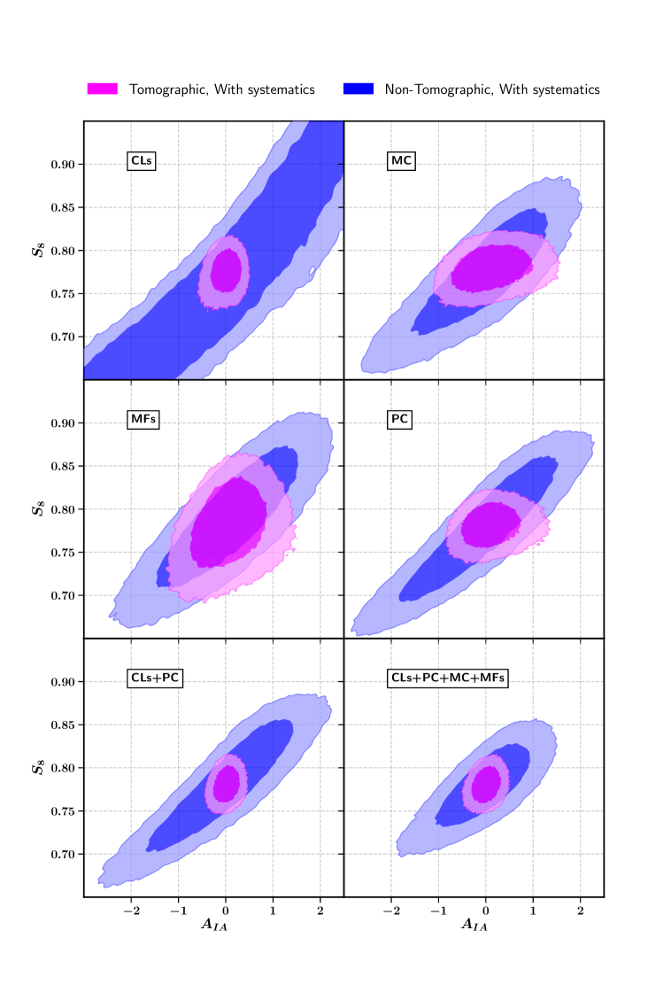
Figure 10: We compare the constraining power of different combinations of statistics in the $A_{\mathrm{IA}}-S_{8}$ plane when inferring cosmology and nuisance parameters simultaneously. While we used a non-tomographic configuration to find the blue constraints, we find the magenta contours using a tomographic setup. Note that since we drew the mock measurement in this study from the fiducial simulations, the contours are centered at the fiducial cosmology. All contours show the 68% and 95 % percentiles of the marginalized 2D-distributions.

6 Conclusions

We conducted a large-scale simulation study on the performance of non-Gaussian mass map statistics, using a realistic stage-3-like WL survey setup. We compare the constraining power in the $\Omega_{\mathrm{m}}-\sigma_{8}$ plane of the angular power spectrum (CLs) with three non-Gaussian statistics, namely; peak counts (PC), minimum counts (MC) and Minkowski functionals (MFs). Our analysis features a multiscale scheme to optimally extract information from the mass maps when using the non-Gaussian statistics. We compare cosmological constraints in a non-tomographic, as well as a tomographic setup, using 4 tomographic bins. Furthermore, we investigate on the robustness of the studied non-Gaussian statistics against the major WL systematic effects, namely; galaxy intrinsic alignment, multiplicative shear bias and photometric redshift error. To avoid having to rely on approximative theory predictions for the non-Gaussian statistics, that limit their usability, we utilize a forward modelling approach to predict the statistics based on a suite of dark-matter-only N-Body simulations.

The main findings of this work include:

• In this setup, we find that the three non-Gaussian statistics considered (PC, MC and MFs) yield stronger constraints in the $\Omega_{\mathrm{m}}-\sigma_{8}$ plane when compared to the angular power spectrum analysis. They experience a less pronounced $\Omega_{\mathrm{m}}-\sigma_{8}$ degeneracy. These findings hold true in a non-tomographic, as well as a tomographic setup. Taking into account galaxy intrinsic alignment, multiplicative shear bias and photometric redshift errors does not change this result. In particular, the PC demonstrate great potential yielding non-tomographic constraints, that are tighter than the constraints found using tomographic CLs, even when galaxy intrinsic alignment is taken into account.

• Including non-Gaussian statistics into the cosmic shear analysis allows us to apply more conservative scale cuts, while conserving the cosmological constraining power. This avoids additional uncertainty in the measurement, arising from the influence of small-scale systematics, in particular baryonic effects. We find competitive constraints by performing a joined analysis using all four studied statistics, considering a conservative range of scales ranging from $\ell=100$ to $\ell=1000$ for the CLs and from 10.5 to 31.6 arcmin for the non-Gaussian statistics.

• While the CLs and the PC experience a significant reduction in constraining power when galaxy intrinsic alignment is taken into account, we find that the MC and MFs are more resilient to it, thanks to a less pronounced degeneracy between $S_{8}$ and $A_{\mathrm{IA}}$.

• We find that the non-Gaussian statistics considered do not profit as much from a tomographic setup as the CLs do. While the cosmological constraining power increases considerably for the CLs, the constraints do not tighten up significantly in case of the non-Gaussian statistics in the absence of systematic effects. If systematic effects are included all statistics profit from the tomographic setup due to the improved constraints on galaxy intrinsic alignment.

• The addition of non-Gaussian statistics to the CLs allows us to find non-tomographic constraints in the $\Omega_{\mathrm{m}}-\sigma_{8}$ plane, that are less than half the size of the constraints found in the tomographic analysis, taking into account galaxy intrinsic alignment, multiplicative shear bias and photometric redshift errors.

• In the context of this study, we developed and distributed a set of Python software tools aimed at simplifying the production of such analyses in the future (namely NGSF, esub-epipe, estats, ekit). A short description of the tools is given in Section 3.7.

This study explored some alternative WL statistics in a forward modelling framework. The introduced simulation framework was developed with a focus on user-friendliness and extendability, allowing to explore a multitude of WL statistics, cosmological parameters and systematic effects.

Since we were only able to study the cosmological constraints in the $\Omega_{\mathrm{m}}-\sigma_{8}$ plane in this study, we plan to extend the number of investigated cosmological parameters in the future and to explore which statistics are most suitable to constrain which parameters.

We plan to extend our study of non-Gaussian statistics, investigating further statistics such as the profiles around peaks/minima, correlations of peaks/minima functions or map moments.

So far we have applied conservative scale cuts, mainly in order to avoid the influence of baryonic effects on small scales. However, the potential of the information contained in the non-linear structure of the matter field on small scales is important. With the non-Gaussian statistics primarily developed to extract this kind of information, the constraining power could be improved, if these scales were considered. Therefore, we plan to include a treatment of baryonic effects in future studies, in order to access the information at smaller scales.

Since none of the non-Gaussian statistics considered was able to put tight constraints on galaxy intrinsic alignment, except for the CL cross-power-spectra, we would like to investigate if cross-correlations between non-Gaussian statistics, measured in different tomographic bins, can put similar or even tighter constraints on galaxy intrinsic alignment.

Lastly, we note that we have considered a simple galaxy intrinsic alignment model in this study, neglecting for example the redshift and luminosity dependence of the effect. We plan to study how the statistics react to a more complex galaxy intrinsic alignment model.

Appendix A Interpolator Test

As described in Section 3.4, we use an interpolator to predict the data-vectors at cosmologies that are not included in the $\Omega_{\mathrm{m}}-\sigma_{8}$ grid sampled with the PKDGRAV3 simulations. We tested, that the error caused by the interpolator does not bias the results significantly. The test was performed by building the interpolator using the simulations for all cosmologies on the sampled grid, except for one cosmology. We then compared the data-vector $d$ at that remaining configuration, as predicted by the simulations directly, to the prediction $d_{\mathrm{interp}}$ of the interpolator for that missing configuration. We repeated this test for each cosmology on the simulated grid. The results of this test are visualized in Figure 11. We found, that the interpolator succeeds in recovering the expected data vectors with an error much smaller than the estimated measurement error for a stage-3-like WL survey for most cosmologies. Therefore, we conclude that the interpolater is unlikely to bias the results significantly. The interpolator fails to recover the expected data-vector for one cosmology only, which is indicated by the black data point in Figure 11. We note, that this cosmology is situated outside of the convex hull of the interpolator, when it is built on the remaining simulations and therefore it is not expected that the interpolator is able to recover the data-vector in this specific case.

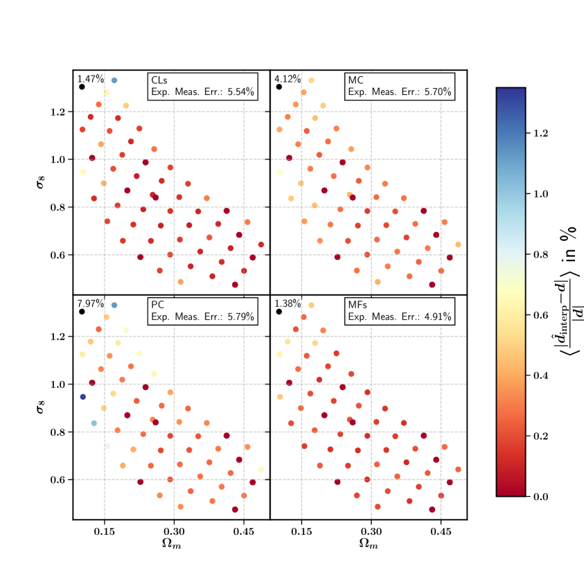
Figure 11: The results of the test performed to asses the performance of the interpolator. Each panel shows the grid of cosmologies sampled with the PKDGRAV3 N-Body simulations for a different statistic. The color indicates the relative error of the interpolator when predicting the data-vector at this cosmology, being built on all simulations but the ones at the cosmology in question. We also denote the estimated measurement error for a stage-3-like survey for each statistic. Note that the black data point lies outside of the convex hull of the interpolator and the prediction of the data-vector corresponds to an extrapolation in this case. The color of this data point does not correspond to the interpolation error, but is indicated directly.

Appendix B Emulator Test

In order to overcome the curse of dimensionality and to make our analysis more easily expandable to a larger grid of cosmological parameters, we develop a semi-analytical emulator to simulate the effects of the systematics on the statistic level directly. In order to avoid biases, caused by the emulator, we require it to recover the true data-vectors with an error smaller than half of the estimated measurement error for a stage-3-like WL survey.

We start from a simple model for the parametric scale factor $a$, introduced in Equation 3.18, containing only 3 parameters

$$a^{i}(\Omega_{\mathrm{m}},\sigma_{8},A_{\mathrm{IA}},m,\Delta_{z}) =c^{i}_{1}A_{\mathrm{IA}}+c^{i}_{2}m+c^{i}_{3}\Delta_{z},$$ (B.1)

where the index $i$ denotes an element of the data-vector. We continuously increased the complexity by adding more terms until the requirement was met for all statistics, ending up with a model containing 16 parameters

$$a^{i}(\Omega_{\mathrm{m}},\sigma_{8},A_{\mathrm{IA}},m,\Delta_{z}) =c^{i}_{1}A_{\mathrm{IA}}+c^{i}_{2}A_{\mathrm{IA}}^{2}+c^{i}_{3}m+c^{i}_{4}m^{2}+c^{i}_{5}\Delta_{z}+c^{i}_{6}\Delta_{z}^{2}$$

$$+c^{i}_{7}A_{\mathrm{IA}}^{2}\Omega_{\mathrm{m}}+c^{i}_{8}A_{\mathrm{IA}}^{2}\sigma_{8}+c^{i}_{9}A_{\mathrm{IA}}\Omega_{\mathrm{m}}\sigma_{8}$$

$$+c^{i}_{10}m\Omega_{\mathrm{m}}+c^{i}_{11}m\sigma_{8}+c^{i}_{12}\Delta_{z}\Omega_{\mathrm{m}}+c^{i}_{13}\Delta_{z}\sigma_{8}$$

$$+c^{i}_{14}A_{\mathrm{IA}}m+c^{i}_{15}m\Delta_{z}+c^{i}_{16}A_{\mathrm{IA}}\Delta_{z}.$$ (B.2)

We found that a sparse sampling of the nuisance parameter space spanned by the parameters $A_{\mathrm{IA}}$, $m$ and $\Delta_{z}$ using $5^{3}$ configurations suffices to model the cross-dependency of the nuisance parameters. To model the dependency on cosmology this sparse sampling of the nuisance parameter space is repeated for 9 different cosmology configurations, distributed on the $\Omega_{\mathrm{m}}-\sigma_{8}$ grid. We tested the performance of the emulator by comparing its predictions to the data-vectors obtained by simulations directly at parameter configurations that are not included in the sub-sample of configurations that are used to fit the emulator. The tests yielding the most critical results, probing the dependency of the systematics on cosmology, as well as the cross-dependency between the systematics themselves, are shown in Figure 12 to 14. The emulator meets our requirements. However, we note that the modelling of the cosmology dependency and the dependency on the other systematics for the galaxy intrinsic alignment, for extreme values of $A_{\mathrm{IA}}$, is not entirely satisfying. Possible reasons for this effect could be the insufficient complexity of the emulator for the galaxy intrinsic alignment part or inaccurate emulation of galaxy intrinsic alignment on the mass map level by the NLA model for extreme values of $A_{\mathrm{IA}}$. While the comparisons in this work are not affected significantly by this effect, it is worth an investigation in future studies.

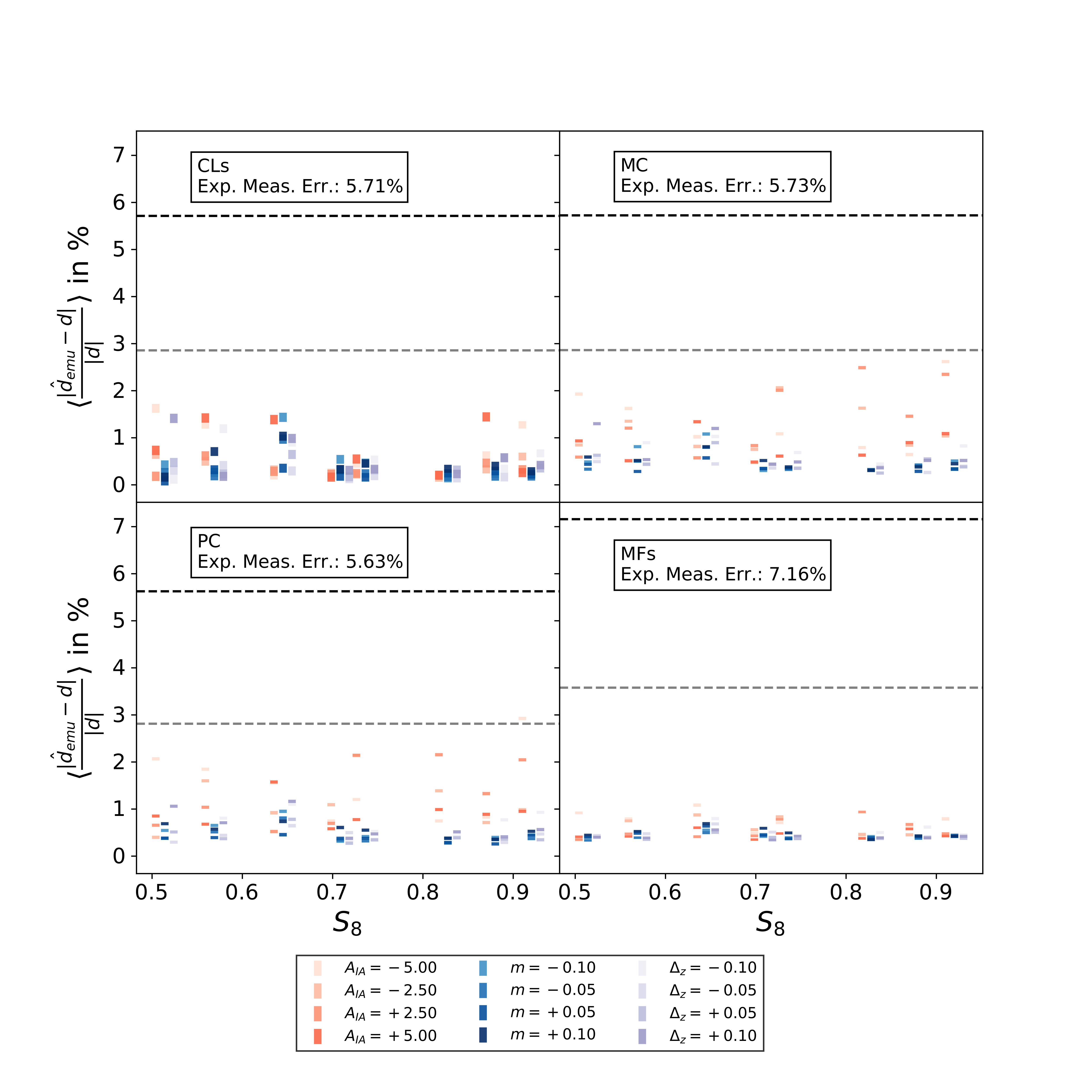
Figure 12: We test how well the emulator is able to recover the dependency of the different systematics on cosmology. To do so, we compare the predictions for the mass map statistics for parameter configurations, that are not included in the samples that are used to build the emulator to the statistics obtained from the simulations directly. In each panel, we show the relative difference between the direct simulation and the emulator prediction. The black dashed line indicates the estimated measurement error for a stage-3-like WL survey, whereas the grey dashed line indicates the requirement for the precision of the emulator corresponding to half the measurement error.

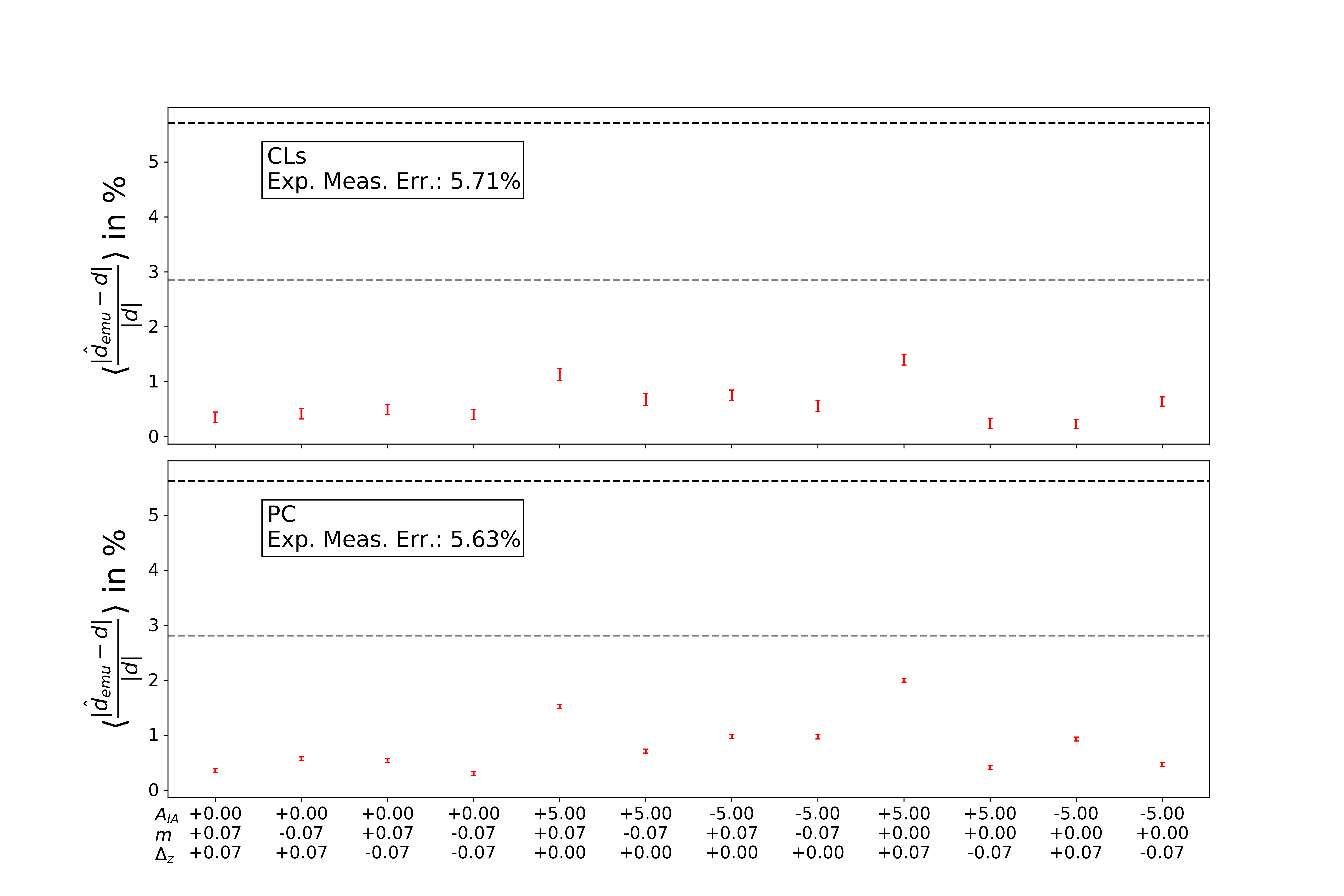
Figure 13: The tests assessing how well the emulator is able to recover the cross-dependencies between different systematics for the CLs and PC. The test is performed by comparing the predictions for the mass map statistics for parameter configurations, that are not included in the samples that are used to build the emulator to the statistics obtained from the simulations directly. All tested configurations are at the fiducial cosmology. In each panel we show the relative difference between the direct simulation and the emulator prediction. The black dashed line indicates the estimated measurement error for a stage-3-like WL survey, whereas the grey dashed line indicates the requirement for the precision of the emulator corresponding to half the measurement error.

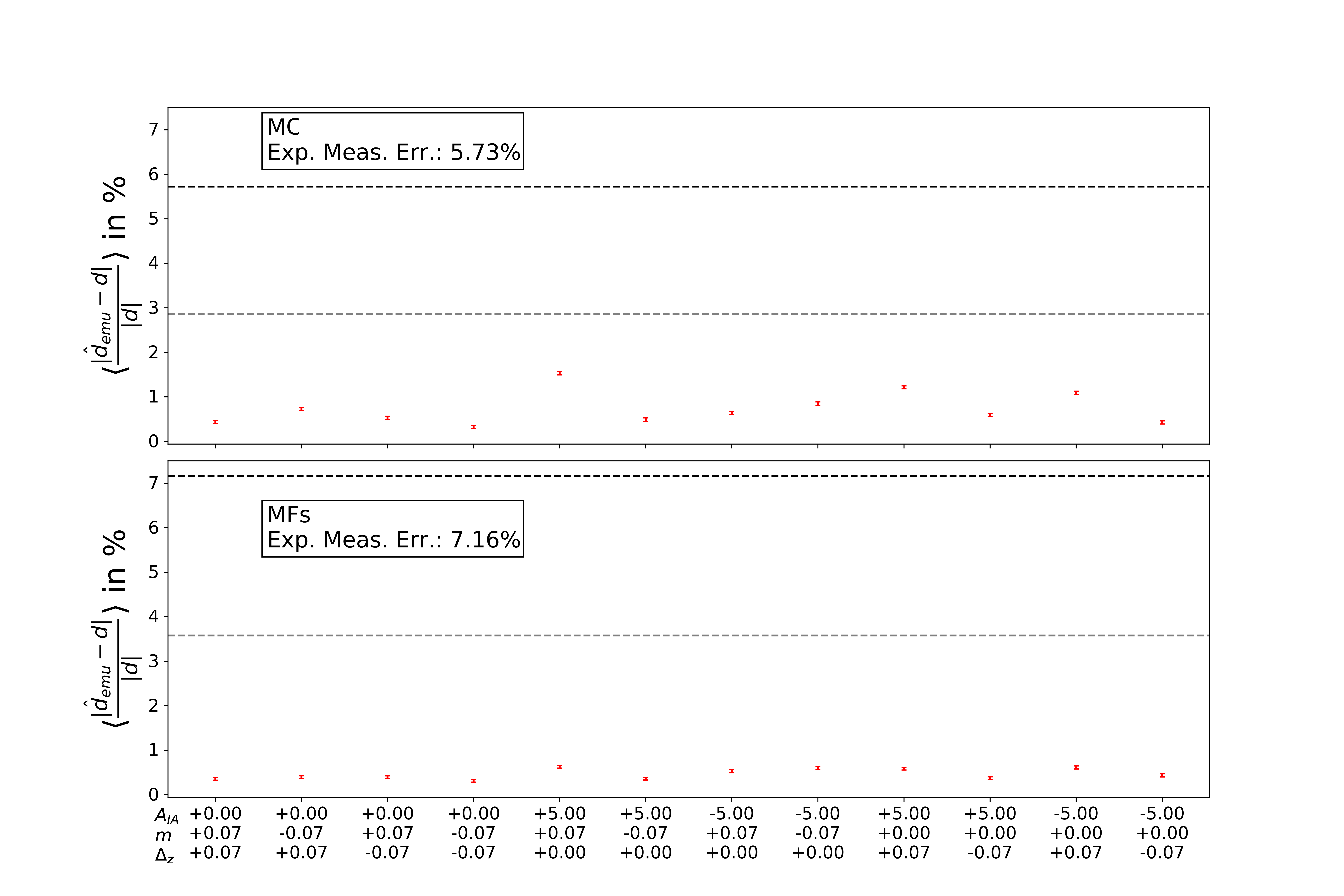
Figure 14: Same as Figure 13, but for the MC and MFs.

References

- [1] B. D. Fields and K. A. Olive, Big bang nucleosynthesis, Nuclear Physics A 777 (2006) 208–225.
- [2] G. Hinshaw, D. Larson, E. Komatsu, D. N. Spergel, C. Bennett, J. Dunkley et al., Nine-year wilkinson microwave anisotropy probe (wmap) observations: cosmological parameter results, The Astrophysical Journal Supplement Series 208 (2013) 19.
- [3] M. Betoule, R. Kessler, J. Guy, J. Mosher, D. Hardin, R. Biswas et al., Improved cosmological constraints from a joint analysis of the sdss-ii and snls supernova samples, Astronomy & Astrophysics 568 (2014) A22.
- [4] A. G. Riess, L. M. Macri, S. L. Hoffmann, D. Scolnic, S. Casertano, A. V. Filippenko et al., A 2.4% determination of the local value of the hubble constant, The Astrophysical Journal 826 (2016) 56.
- [5] A. G. Riess, S. Casertano, W. Yuan, L. Macri, B. Bucciarelli, M. G. Lattanzi et al., Milky way cepheid standards for measuring cosmic distances and application to gaia dr2: implications for the hubble constant, The Astrophysical Journal 861 (2018) 126.
- [6] V. Bonvin, F. Courbin, S. H. Suyu, P. Marshall, C. Rusu, D. Sluse et al., H0licow–v. new cosmograil time delays of he 0435- 1223: H0 to 3.8 per cent precision from strong lensing in a flat cdm model, Monthly Notices of the Royal Astronomical Society 465 (2017) 4914–4930.
- [7] S. Birrer, T. Treu, C. Rusu, V. Bonvin, C. Fassnacht, J. Chan et al., H0licow–ix. cosmographic analysis of the doubly imaged quasar sdss 1206+ 4332 and a new measurement of the hubble constant, Monthly Notices of the Royal Astronomical Society 484 (2019) 4726–4753.
- [8] P. A. Ade, N. Aghanim, M. Arnaud, M. Ashdown, J. Aumont, C. Baccigalupi et al., Planck 2015 results-xiii. cosmological parameters, Astronomy & Astrophysics 594 (2016) A13.
- [9] N. Aghanim, Y. Akrami, M. Ashdown, J. Aumont, C. Baccigalupi, M. Ballardini et al., Planck 2018 results. vi. cosmological parameters, arXiv preprint arXiv:1807.06209 (2018) .
- [10] M. Kilbinger, Cosmology with cosmic shear observations: a review, Reports on Progress in Physics 78 (2015) 086901.
- [11] D. E. T. Force, Report of the dark energy task force, Available online from NSF (2006) .
- [12] C. Heymans, E. Grocutt, A. Heavens, M. Kilbinger, T. D. Kitching, F. Simpson et al., Cfhtlens tomographic weak lensing cosmological parameter constraints: Mitigating the impact of intrinsic galaxy alignments, Monthly Notices of the Royal Astronomical Society 432 (2013) 2433–2453.
- [13] E. M. Huff, T. Eifler, C. Hirata, R. Mandelbaum, D. Schlegel and U. Seljak, A cosmic shear measurement from sdss, in American Astronomical Society Meeting Abstracts# 219, vol. 219, 2012.
- [14] T. Abbott, F. B. Abdalla, A. Alarcon, J. Aleksić, S. Allam, S. Allen et al., Dark energy survey year 1 results: Cosmological constraints from galaxy clustering and weak lensing, Physical Review D 98 (2018) 043526.
- [15] H. Hildebrandt, M. Viola, C. Heymans, S. Joudaki, K. Kuijken, C. Blake et al., Kids-450: Cosmological parameter constraints from tomographic weak gravitational lensing, Monthly Notices of the Royal Astronomical Society 465 (2016) 1454–1498.
- [16] C. Hikage, M. Oguri, T. Hamana, S. More, R. Mandelbaum, M. Takada et al., Cosmology from cosmic shear power spectra with subaru hyper suprime-cam first-year data, Publications of the Astronomical Society of Japan 71 (2019) 43.
- [17] P. A. Abell, D. L. Burke, M. Hamuy, M. Nordby, T. S. Axelrod, D. Monet et al., Lsst science book, version 2.0, tech. rep., 2009.
- [18] L. Amendola, S. Appleby, A. Avgoustidis, D. Bacon, T. Baker, M. Baldi et al., Cosmology and fundamental physics with the euclid satellite, Living reviews in relativity 21 (2018) 2.
- [19] X. Yang, J. M. Kratochvil, K. Huffenberger, Z. Haiman and M. May, Baryon impact on weak lensing peaks and power spectrum: Low-bias statistics and self-calibration in future surveys, Physical Review D 87 (2013) 023511.
- [20] K. Osato, M. Shirasaki and N. Yoshida, Impact of baryonic processes on weak-lensing cosmology: Power spectrum, nonlocal statistics, and parameter bias, The Astrophysical Journal 806 (2015) 186.
- [21] A. Heavens, A. Refregier and C. Heymans, Intrinsic correlation of galaxy shapes: implications for weak lensing measurements, Monthly Notices of the Royal Astronomical Society 319 (2000) 649–656.
- [22] L. Voigt and S. Bridle, Limitations of model-fitting methods for lensing shear estimation, Monthly Notices of the Royal Astronomical Society 404 (2010) 458–467.
- [23] C. Bonnett, M. Troxel, W. Hartley, A. Amara, B. Leistedt, M. Becker et al., Redshift distributions of galaxies in the des science verification shear catalogue and implications for weak lensing, arXiv preprint arXiv:1507.05909 (2015) .
- [24] N. MacCrann, J. Zuntz, S. Bridle, B. Jain and M. R. Becker, Cosmic discordance: are planck cmb and cfhtlens weak lensing measurements out of tune?, Monthly Notices of the Royal Astronomical Society 451 (2015) 2877–2888.
- [25] A. Petri, M. May, Z. Haiman and J. M. Kratochvil, Impact of spurious shear on cosmological parameter estimates from weak lensing observables, Physical Review D 90 (2014) 123015.
- [26] E. Semboloni, T. Schrabback, L. van Waerbeke, S. Vafaei, J. Hartlap and S. Hilbert, Weak lensing from space: first cosmological constraints from three-point shear statistics, Monthly Notices of the Royal Astronomical Society 410 (2011) 143–160.
- [27] A. Cooray and W. Hu, Weak gravitational lensing bispectrum, The Astrophysical Journal 548 (2001) 7.
- [28] M. Takada and B. Jain, Cosmological parameters from lensing power spectrum and bispectrum tomography, Monthly Notices of the Royal Astronomical Society 348 (2004) 897–915.
- [29] B. Jain and U. Seljak, Cosmological model predictions for weak lensing: Linear and nonlinear regimes, The Astrophysical Journal 484 (1997) 560.
- [30] M. Gatti, C. Chang, O. Friedrich, B. Jain, D. Bacon, M. Crocce et al., Dark energy survey year 3 results: cosmology with moments of weak lensing mass maps–validation on simulations, arXiv preprint arXiv:1911.05568 (2019) .
- [31] C. Chang, A. Pujol, B. Mawdsley, D. Bacon, J. Elvin-Poole, P. Melchior et al., Dark energy survey year 1 results: curved-sky weak lensing mass map, Monthly Notices of the Royal Astronomical Society 475 (2018) 3165–3190.
- [32] K. Patton, J. Blazek, K. Honscheid, E. Huff, P. Melchior, A. J. Ross et al., Cosmological constraints from the convergence 1-point probability distribution, Monthly Notices of the Royal Astronomical Society 472 (2017) 439–446.
- [33] J. M. Kratochvil, Z. Haiman and M. May, Probing cosmology with weak lensing peak counts, Physical Review D 81 (2010) 043519.
- [34] J. Liu, A. Petri, Z. Haiman, L. Hui, J. M. Kratochvil and M. May, Cosmology constraints from the weak lensing peak counts and the power spectrum in cfhtlens data, Physical Review D 91 (2015) 063507.
- [35] T. Kacprzak, D. Kirk, O. Friedrich, A. Amara, A. Refregier, L. Marian et al., Cosmology constraints from shear peak statistics in dark energy survey science verification data, Monthly Notices of the Royal Astronomical Society 463 (2016) 3653–3673.
- [36] C. Sánchez, J. Clampitt, A. Kovacs, B. Jain, J. García-Bellido, S. Nadathur et al., Cosmic voids and void lensing in the dark energy survey science verification data, Monthly Notices of the Royal Astronomical Society (2016) stw2745.
- [37] D. Gruen, O. Friedrich, A. Amara, D. Bacon, C. Bonnett, W. Hartley et al., Weak lensing by galaxy troughs in des science verification data, Monthly Notices of the Royal Astronomical Society 455 (2016) 3367–3380.
- [38] W. R. Coulton, J. Liu, I. G. McCarthy and K. Osato, Weak lensing minima and peaks: Cosmological constraints and the impact of baryons, arXiv preprint arXiv:1910.04171 (2019) .
- [39] J. M. Kratochvil, E. A. Lim, S. Wang, Z. Haiman, M. May and K. Huffenberger, Probing cosmology with weak lensing minkowski functionals, Physical Review D 85 (2012) 103513.
- [40] A. Petri, J. Liu, Z. Haiman, M. May, L. Hui and J. M. Kratochvil, Emulating the cfhtlens weak lensing data: Cosmological constraints from moments and minkowski functionals, Physical Review D 91 (2015) 103511.
- [41] S. Bridle and L. King, Dark energy constraints from cosmic shear power spectra: impact of intrinsic alignments on photometric redshift requirements, New Journal of Physics 9 (2007) 444.
- [42] J. T. Giblin Jr, J. B. Mertens, G. D. Starkman and A. R. Zentner, General relativistic corrections to the weak lensing convergence power spectrum, Physical Review D 96 (2017) 103530.
- [43] M. Maturi, C. Angrick, F. Pace and M. Bartelmann, An analytic approach to number counts of weak-lensing peak detections, Astronomy & Astrophysics 519 (2010) A23.
- [44] C. Parroni, V. F. Cardone, R. Maoli and R. Scaramella, Going deep with minkowski functionals of convergence maps, Astronomy & Astrophysics 633 (2020) A71.
- [45] M. Bartelmann and P. Schneider, Weak gravitational lensing, Physics Reports 340 (2001) 291–472.
- [46] D. Huterer, M. Takada, G. Bernstein and B. Jain, Systematic errors in future weak-lensing surveys: requirements and prospects for self-calibration, Monthly Notices of the Royal Astronomical Society 366 (2006) 101–114.
- [47] C. G. Wallis, J. D. McEwen, T. D. Kitching, B. Leistedt and A. Plouviez, Mapping dark matter on the celestial sphere with weak gravitational lensing, arXiv preprint arXiv:1703.09233 (2017) .
- [48] N. Kaiser and G. Squires, Mapping the dark matter with weak gravitational lensing, The Astrophysical Journal 404 (1993) 441–450.
- [49] J. Fluri, T. Kacprzak, R. Sgier, A. Refregier and A. Amara, Weak lensing peak statistics in the era of large scale cosmological surveys, Journal of Cosmology and Astroparticle Physics 2018 (2018) 051.
- [50] P. J. E. Peebles, The large-scale structure of the universe. Princeton university press, 1980.
- [51] A. Nicola, A. Refregier, A. Amara and A. Paranjape, Three-dimensional spherical analyses of cosmological spectroscopic surveys, Physical Review D 90 (2014) 063515.
- [52] D. N. Limber, The analysis of counts of the extragalactic nebulae in terms of a fluctuating density field., The Astrophysical Journal 117 (1953) 134.
- [53] J. A. Tyson, F. Valdes and R. Wenk, Detection of systematic gravitational lens galaxy image alignments-mapping dark matter in galaxy clusters, The Astrophysical Journal 349 (1990) L1–L4.
- [54] J. Miralda-Escude, The correlation function of galaxy ellipticities produced by gravitational lensing, The Astrophysical Journal 380 (1991) 1–8.
- [55] P. Schneider, Detection of (dark) matter concentrations via weak gravitational lensing, Monthly Notices of the Royal Astronomical Society 283 (1996) 837–853.
- [56] K. Reblinsky, G. Kruse, B. Jain and P. Schneider, Cosmic shear and halo abundances: analytical versus numerical results, arXiv preprint astro-ph/9907250 (1999) .
- [57] J. Liu and Z. Haiman, Origin of weak lensing convergence peaks, Physical Review D 94 (2016) 043533.
- [58] L. Marian, R. E. Smith, S. Hilbert and P. Schneider, The cosmological information of shear peaks: beyond the abundance, Monthly Notices of the Royal Astronomical Society 432 (2013) 1338–1350.
- [59] J. Berge, A. Amara and A. Refregier, Optimal capture of non-gaussianity in weak-lensing surveys: Power spectrum, bispectrum, and halo counts, The Astrophysical Journal 712 (2010) 992.
- [60] T. Baker, J. Clampitt, B. Jain and M. Trodden, Void lensing as a test of gravity, Physical Review D 98 (2018) 023511.
- [61] E. Paillas, M. Cautun, B. Li, Y.-C. Cai, N. Padilla, J. Armijo et al., The santiago–harvard–edinburgh–durham void comparison ii: unveiling the vainshtein screening using weak lensing, Monthly Notices of the Royal Astronomical Society 484 (2019) 1149–1165.
- [62] K. Mecke, Buchert; t. & wagner, h., 1994, Astron. Astrophys 288 697.
- [63] M. Vicinanza, V. F. Cardone, R. Maoli, R. Scaramella, X. Er and I. Tereno, Minkowski functionals of convergence maps and the lensing figure of merit, Physical Review D 99 (2019) 043534.
- [64] H. Tomita, Curvature invariants of random interface generated by gaussian fields, Progress of Theoretical Physics 76 (1986) 952–955.
- [65] A. Petri, Z. Haiman, L. Hui, M. May and J. M. Kratochvil, Cosmology with minkowski functionals and moments of the weak lensing convergence field, Physical Review D 88 (2013) 123002.
- [66] M. A. Troxel, N. MacCrann, J. Zuntz, T. Eifler, E. Krause, S. Dodelson et al., Dark energy survey year 1 results: Cosmological constraints from cosmic shear, Physical Review D 98 (2018) 043528.
- [67] C. Bruderer, C. Chang, A. Refregier, A. Amara, J. Bergé and L. Gamper, Calibrated ultra fast image simulations for the dark energy survey, The Astrophysical Journal 817 (2016) 25.
- [68] I. Smail, D. W. Hogg, L. Yan and J. G. Cohen, Deep optical galaxy counts with the keck telescope, The Astrophysical Journal Letters 449 (1995) L105.
- [69] A. Amara and A. Réfrégier, Optimal surveys for weak-lensing tomography, Monthly Notices of the Royal Astronomical Society 381 (2007) 1018–1026.
- [70] D. Potter, J. Stadel and R. Teyssier, Pkdgrav3: beyond trillion particle cosmological simulations for the next era of galaxy surveys, Computational Astrophysics and Cosmology 4 (2017) 2.
- [71] T. Tram, J. Brandbyge, J. Dakin and S. Hannestad, Fully relativistic treatment of light neutrinos in n-body simulations, Journal of Cosmology and Astroparticle Physics 2019 (2019) 022.
- [72] J. Fluri, T. Kacprzak, A. Lucchi, A. Refregier, A. Amara, T. Hofmann et al., Cosmological constraints with deep learning from kids-450 weak lensing maps, Physical Review D 100 (2019) 063514.
- [73] R. J. Sgier, A. Réfrégier, A. Amara and A. Nicola, Fast generation of covariance matrices for weak lensing, Journal of Cosmology and Astroparticle Physics 2019 (2019) 044.
- [74] R. Teyssier, S. Pires, S. Prunet, D. Aubert, C. Pichon, A. Amara et al., Full-sky weak-lensing simulation with 70 billion particles, Astronomy & Astrophysics 497 (2009) 335–341.
- [75] S. Pires, J.-L. Starck, A. Amara, A. Réfrégier and R. Teyssier, Cosmological model discrimination with weak lensing, Astronomy & Astrophysics 505 (2009) 969–979.
- [76] J. Schmelzle, A. Lucchi, T. Kacprzak, A. Amara, R. Sgier, A. Réfrégier et al., Cosmological model discrimination with deep learning, arXiv preprint arXiv:1707.05167 (2017) .
- [77] K. M. Gorski, B. D. Wandelt, F. K. Hansen, E. Hivon and A. J. Banday, The healpix primer, arXiv preprint astro-ph/9905275 (1999) .
- [78] E. Sellentin and A. F. Heavens, Parameter inference with estimated covariance matrices, Monthly Notices of the Royal Astronomical Society: Letters 456 (2015) L132–L136.
- [79] N. Jeffrey and F. B. Abdalla, Parameter inference and model comparison using theoretical predictions from noisy simulations, Monthly Notices of the Royal Astronomical Society 490 (2019) 5749–5756.
- [80] D. Foreman-Mackey, D. W. Hogg, D. Lang and J. Goodman, emcee: the mcmc hammer, Publications of the Astronomical Society of the Pacific 125 (2013) 306.
- [81] E. Jones, T. Oliphant and P. Peterson, Scipy: Open source scientific tools for python, .
- [82] S. v. d. Walt, S. C. Colbert and G. Varoquaux, The numpy array: a structure for efficient numerical computation, Computing in Science & Engineering 13 (2011) 22–30.
- [83] C. M. Hirata and U. Seljak, Intrinsic alignment-lensing interference as a contaminant of cosmic shear, Physical Review D 70 (2004) 063526.
- [84] B. Joachimi, R. Mandelbaum, F. Abdalla and S. Bridle, Constraints on intrinsic alignment contamination of weak lensing surveys using the megaz-lrg sample, Astronomy & Astrophysics 527 (2011) A26.
- [85] H. Hildebrandt, M. Viola, C. Heymans, S. Joudaki, K. Kuijken, C. Blake et al., Kids-450: Cosmological parameter constraints from tomographic weak gravitational lensing, Monthly Notices of the Royal Astronomical Society 465 (2017) 1454–1498.
- [86] A. Refregier, T. Kacprzak, A. Amara, S. Bridle and B. Rowe, Noise bias in weak lensing shape measurements, Monthly Notices of the Royal Astronomical Society 425 (2012) 1951–1957.
- [87] G. M. Bernstein, Shape measurement biases from underfitting and ellipticity gradients, Monthly Notices of the Royal Astronomical Society 406 (2010) 2793–2804.
- [88] S. Paulin-Henriksson, A. Refregier and A. Amara, Optimal point spread function modeling for weak lensing: complexity and sparsity, Astronomy & Astrophysics 500 (2009) 647–655.
- [89] H. Hildebrandt, F. Köhlinger, J. van den Busch, B. Joachimi, C. Heymans, A. Kannawadi et al., Kids+ viking-450: Cosmic shear tomography with optical and infrared data, Astronomy & Astrophysics 633 (2020) A69.
- [90] A. J. Weiss, A. Schneider, R. Sgier, T. Kacprzak, A. Amara and A. Refregier, Effects of baryons on weak lensing peak statistics, Journal of Cosmology and Astroparticle Physics 2019 (2019) 011.
- [91] J. Blazek, Z. Vlah and U. Seljak, Tidal alignment of galaxies, Journal of Cosmology and Astroparticle Physics 2015 (2015) 015.
- [92] J. A. Blazek, N. MacCrann, M. Troxel and X. Fang, Beyond linear galaxy alignments, Physical Review D 100 (2019) 103506.
- [93] P. Virtanen, R. Gommers, T. E. Oliphant, M. Haberland, T. Reddy, D. Cournapeau et al., Scipy 1.0: fundamental algorithms for scientific computing in python, Nature methods 17 (2020) 261–272.
- [94] J. D. Hunter, Matplotlib: A 2d graphics environment, Computing in science & engineering 9 (2007) 90–95.
- [95] A. Lewis, Getdist: a python package for analysing monte carlo samples, arXiv preprint arXiv:1910.13970 (2019) .