The GCE in a New Light: Disentangling the -ray Sky with Bayesian Graph Convolutional Neural Networks
Abstract
A fundamental question regarding the Galactic Center Excess (GCE) is whether the underlying structure is point-like or smooth. This debate, often framed in terms of a millisecond pulsar or annihilating dark matter (DM) origin for the emission, awaits a conclusive resolution. In this work we weigh in on the problem using Bayesian graph convolutional neural networks. In simulated data, our neural network (NN) is able to reconstruct the flux of inner Galaxy emission components to on average 0.5%, comparable to the non-Poissonian template fit (NPTF). When applied to the actual Fermi-LAT data, we find that the NN estimates for the flux fractions from the background templates are consistent with the NPTF; however, the GCE is almost entirely attributed to smooth emission. While suggestive, we do not claim a definitive resolution for the GCE, as the NN tends to underestimate the flux of point-sources peaked near the 1 detection threshold. Yet the technique displays robustness to a number of systematics, including reconstructing injected DM, diffuse mismodeling, and unmodeled north-south asymmetries. So while the NN is hinting at a smooth origin for the GCE at present, with further refinements we argue that Bayesian Deep Learning is well placed to resolve this DM mystery.
Introduction.—
Dark Matter (DM) annihilation into highly energetic standard model particles is a central prediction of well-motivated theories, including weakly interacting massive particles (WIMPs) [1]. Due to its high DM density and relative proximity, the center of the Milky Way is a promising location to search for the annihilation products, and in fact, the Fermi -ray telescope observes excess emission from the inner region of the Milky Way that could be accommodated by annihilation from thermal WIMPs [2, 3, 4, 5, 6, 7, 8, 9, 10, 11, 12, 13, 14, 15]. Since its discovery in 2009, a DM origin of this Galactic Center Excess (GCE) has been disputed, and arguments have been raised in favor of a population of millisecond pulsars (e.g. [3, 5, 16, 8, 17, 18, 19, 20]), emission from unmodeled cosmic rays (e.g. [21, 22, 23]), and that the emission may be more accurately correlated with stellar overdensities towards the Galactic Center (GC; e.g. [14, 24, 25, 26, 27]). The case for millisecond pulsars is based on evidence from two methods: wavelet techniques [28, 29, 30] and the non-Poissonian template fit (NPTF) [31, 32, 33, 34]. It has been strongly argued that both methods prefer the emission to possess the small scale structure indicative of a point-source (PS) origin, rather than the smooth photon map (up to Poisson fluctuations) predicted by annihilating DM. Yet as with any inner Galaxy analysis, dependence upon systematic uncertainties is key. When masking more recently identified PSs near the GC, additional wavelet peaks associated with the GCE flux are no longer detected [35] (cf. [36]). Further, the NPTF can be biased in favor of PSs when there is an unmodeled north-south asymmetry [37, 38]. The method also appeared unable to recover an injected DM signal [39], although such behavior can be expected to a degree when the flux is a mixture of smooth and PS emission [40], and can largely be resolved through the use of either improved diffuse models or harmonic marginalization [36]. The more recent studies have emphasized that there is an ambiguity inherent in the physics: emission from sufficiently dim PSs is exactly Poissonian, and hence formally indistinguishable from the expected DM signal. Whether the GCE has a DM or PS origin is therefore only a well defined question for sufficiently bright PSs. In short, while we continue to learn more about the GCE and the systematic dependence of existing methods, the possibility that there is a hint of the particle nature of DM in the inner Galaxy remains.
An alternative powerful approach to the problem that intrinsically utilizes inter-pixel correlations and autonomously determines the characteristic features of each template is given by convolutional neural networks (CNNs). Since a natural format for the Fermi-LAT data is the HEALPix tessellation of the sphere [41], we base our NN on the DeepSphere architecture [42, 43]. By training on a large number of diverse photon-count maps, our NN learns to predict the flux fractions associated with the different emission components. We implement the approach of Ref. [44] to render our NN a Bayesian Graph Convolutional Neural Network (Bayesian GCNN); thus, the NN learns a distribution of each NN weight, rather than only a single value, which enables the estimation of uncertainties.
Using this framework, we demonstrate that CNNs are a significant competitor for resolving the GCE debate. The method is capable of learning the central physics of template fitting: accurately estimating the flux fractions of all the templates that compose the photon-count map (cf. [45] where CNNs were used to estimate contributions to the GCE alone). In most cases our NN recovers the GCE flux contributions to the percent level and is robust to key systematics, including a degree of diffuse mismodeling and unmodeled asymmetries. When applied to the real Fermi data, the method reports flux fractions consistent with the the NPTF for all components, differing only in the composition of the GCE: while the NPTF attributes 100% of the GCE flux to PSs for our modeling choices, the CNN prefers an almost entirely smooth origin. While suggestive, our results also exhibit signs of the inherent PS and DM degeneracy at play, and in systematic studies we find cases where there can be bias towards the smooth template. As such, we stop short of declaring a resolution of the GCE origin with this method, but instead claim the method as having the clear potential to do so.
This Letter is structured as follows. First, we briefly describe the Fermi data set and the generation of mock data used for training the NN. Then, we summarize the DeepSphere framework that forms the backbone of our Bayesian GCNN. We introduce the concepts of aleatoric and epistemic uncertainty in the context of Bayesian Deep Learning and discuss how their estimation can be naturally embedded into the training process of the NN. Moreover, we outline the architecture of our NN. We evaluate the performance of our NN in a proof-of-concept example with simulated maps composed of photon counts from smooth and/or PS GCE emission together with four background templates and compare our results with those from the NPTFit [34] implementation of the NPTF. Finally, we analyze the predictions of our NN for simulated mock maps of the GC that correspond to the best-fit parameters as determined by NPTFit and for the real Fermi data. Supporting results and a detailed discussion of the systematics of the method can be found in the Supplementary Material (SM).
Data selection and generation.—
We use the Pass 8 Fermi photon counts within a reconstructed energy range of that have been detected between Aug 4, 2008 and July 7, 2016. We select events within the highest cosmic-ray rejection class, UltraCleanVeto, and apply the quality cuts DATA_QUAL==1, LAT_CONFIG==1, and zenith angle . This exact data set has previously been employed in [34, 46, 36]. We model the inner Galaxy using the following Poissonian templates: (1) isotropic background accounting for extragalactic emission and cosmic ray contamination, (2) uniform emission from the Fermi bubbles [47], (3) Galactic diffuse background from neutral pions decaying into photons and from bremsstrahlung, (4) Galactic diffuse background from inverse Compton scattering, and (5) GCE due to annihilating DM. For the diffuse background components, by default we choose Model O, which was introduced in [36] (building on [14, 26]), and has been shown to remedy mismodeling concerns raised in [39]. The template for the GCE is taken to be the line-of-sight integral through the square of a generalized Navarro–Frenk–White (NFW) profile [48], i.e. , with inner slope and scale radius (see e.g. [9]). Additionally, we assume contributions from two PS templates: (6) NFW-squared PSs that serve as an alternative explanation for the GCE, and (7) disk-correlated PSs described by a doubly exponential disk with scale height and radius . All maps are given resolution .
CNNs are supervised learning methods, and determine a generalizable mapping between input (photon-count maps) and output (flux fraction of each template) by seeing a large number of input training samples alongside the corresponding output. For both the proof-of-concept example and the realistic scenario, we create 600,000 training maps using the publicly available tool NPTFit-Sim [49] for the PS templates (accounting for the Fermi point spread function) and sampling from Poisson distributions with pixel-wise means set by each exposure-corrected Poissonian template. We randomly draw all template parameters from wide prior distributions. In this way, our NN is trained to estimate the flux fractions in arbitrarily composed maps (which may contain PSs described by any source count distribution (SCD) whose NPTF parameters lie within the prior cube), but narrower priors around the expected Fermi values are considered in the SM, giving very similar results for the Fermi map. We model the PSs with singly-broken power laws with variable slopes, spanning the entire relevant brightness range from the 3FGL detection threshold down to very faint PSs. Just like the NPTF, our method is agnostic about the physical nature of the PSs (see the SM for an application to a SCD derived from millisecond pulsars, which are the most popular candidate for PS emission).
Bayesian graph convolutional neural networks.—
CNNs [50], and more recently Bayesian variants, have been applied to a range of problems in cosmology, see e.g. [51, 52, 53]. They consist of multiple layers that successively map an input to an output . The core layers possess weights , free parameters that are updated in the course of the NN training by means of a stochastic gradient descent algorithm in order to minimize the expected loss. Thus, the objective of the training is to find
| (1) | ||||
where and denote the samples and true labels of the training data, respectively, and is a loss function that measures the fidelity of the NN output with respect to the truth for an arbitrary input map given the weights . The expectation value in the first line is taken over the joint distribution of , which in practice is approximated by minimizing the average loss across a large number of training samples drawn from the joint distribution of . The main building block of CNNs is the eponymous convolution operation, which in the DeepSphere approach is defined in Fourier space by resorting to the graph Laplacian operator. During the NN training, these convolutional kernels are gradually updated and learn to extract relevant features in the data. While the first convolutional layer tends to detect low-level features such as gradients and edges, stacking several convolutional layers (as done in “Deep Learning”) enables the NN to recognize more involved structures in the data.
Estimating uncertainties.—
While finding such that is sufficient in many applications, estimating the uncertainties of the flux fractions predicted is vital in interpreting the results. Following Refs. [54, 55, 44], we distinguish between data-inherent aleatoric (statistical) uncertainty, which is innate in the photon-count maps due to the stochasticity of the -ray emission from different origins that is detected in each pixel, and model-related epistemic (systematic) uncertainty, which describes the ignorance about how well the NN approximates the correct input-to-output mapping.
Aleatoric uncertainty is inherent to each photon-count map and hence cannot be reduced by increasing the number of training samples. Since we expect the noise level to vary among the samples depending on the number of photons and the contributing templates (for instance, PS emission becomes degenerate with Poissonian emission in the ultrafaint limit), we model the aleatoric uncertainty to be heteroscedastic, i.e. dependent on the specific photon-count map (). Rather than assuming a noise level a priori, we train the NN to predict the aleatoric noise. For this purpose, we assume that the uncertainty of each flux fraction can be reasonably described by a multivariate Gaussian with diagonal covariance matrix , where stands for the number of templates.111The extension to non-diagonal uncertainty covariance matrices is treated in the SM. We take the negative maximum log-likelihood estimate for the pair as the loss function in Eq. (1), given by
| (2) |
and use a final NN layer with output dimension for predicting , where . As the NN itself estimates , also depends on the weights . The terms with in the numerator and denominator in (2) favor small and large values for , respectively, with the optimal balancing the two.
For estimating the epistemic uncertainty, we use Concrete Dropout [55]. While the original motivation of randomly zeroing NN units is to prevent overfitting [56, 57], it has been shown that this Dropout can be viewed as a Bayesian approximation of the posterior distribution for the NN weights [54]. Since this distribution is in general analytically intractable, it is approximated by a simpler distribution that minimizes the Kullback–Leibler divergence , or equivalently maximizes the evidence lower bound. Applying Dropout at test time can then be interpreted as sampling weights from . Whereas well-calibrated Dropout probabilities can be determined with a grid search, Concrete Dropout lets the NN autonomously adapt the Dropout probabilities during the training.
Neural network architecture and training.—
Our NN processes the input maps with 7 consecutive graph convolutional layers that act as feature extractors, each of which is followed by a batch normalization operation [58], a ReLU non-linearity, and a max-pooling operation, which reduces the parameter by a factor of 2 and therefore the number of pixels by 4, whereas the number of channels (also called feature maps, which are associated with individual sets of convolutional kernels) gradually increases from 32 after the first graph convolutional layer to a maximum of 256. Thereafter, we employ two fully connected layers with ReLU activation and a final fully connected layer with output neurons for the means and log-variances, where we use a Softmax activation for the means in order to enforce the flux fractions to lie in and to sum to unity. The details are supplied in the SM. In total, our implementation of the Bayesian GCNN in Tensorflow [59] has roughly trainable parameters. We use a batch size of and take an Adam optimizer [60] with learning rate decaying with a rate of with respect to mini-batch iterations. We train the NN by performing 30,000 mini-batch iterations (25,000 for the proof-of-concept example) on a single Nvidia Tesla Volta V100 GPU on the supercomputer Gadi, which is located in Canberra and is part of the National Computational Infrastructure (NCI), taking roughly two hours for the realistic scenario.
Proof-of-concept example: recovering the GCE flux fractions from simulated maps.—
In this example, we consider the recovery of the flux fractions for the following scenario: all the Poissonian templates are present and we include the GCE PS as the only PS template. Importantly, this setup is representative of the challenges we will encounter in the real data as we never encounter systematic confusion between the GCE and disk PS models, as demonstrated in the SM. We take a fixed ROI of around the GC, with the Galactic Plane masked at latitudes . We do not estimate uncertainties in this benchmark example but rather compare the NN predictions with the true values and with the estimates from NPTFit. Therefore, we train the NN with a simple loss. The nested sampling in NPTFit is done using MultiNest [61, 62] with 500 live points. To speed up NPTFit, we choose a uniform exposure map with Fermi mean exposure in this example.
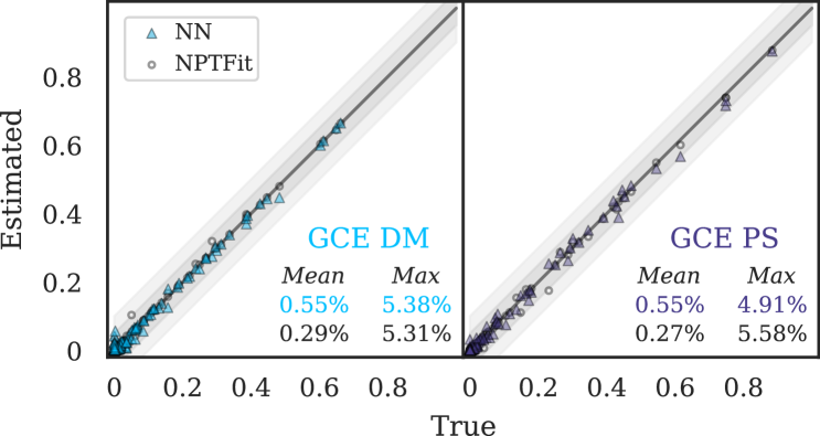
Fig. 1 depicts the true vs. estimated flux fractions for the NN and NPTFit, for 172 out of 256 randomly composed maps from the testing data set (not seen by the NN during the training) for which NPTFit converged.222This criterion was established to account for simulated maps with a large number of counts-per-pixel, where the current implementation of the NPTF in NPTFit fails. Here we imposed a simple cut of rejecting cases where NPTFit failed to converge in a fixed run time. This is sufficient for a qualitative comparison between the method and the NN output. Nevertheless, we caution that this has undoubtedly biased the detailed results depicted, likely in favor of NPTFit. We discuss this point further in the SM. For NPTFit, we report the medians of the flux fraction posterior distributions. The errors for both the NN and NPTFit estimates are on average well below one per cent for all the templates (including those not shown), and the maximum errors are comparable. In the SM, we demonstrate that the NN displays robustness in distinguishing GCE DM and PS in the presence of diffuse mismodeling and an unmodeled north-south asymmetry of the GCE (a case where NPTFit can be biased [37, 38]). Nonetheless, we caution that when the peak of the PS distribution tends towards the detection threshold, there can be systematic confusion between GCE DM and PS, particularly if the flux arises from a mixture of both, as seen also with NPTFit [40].
Application to the Fermi-LAT count map.—
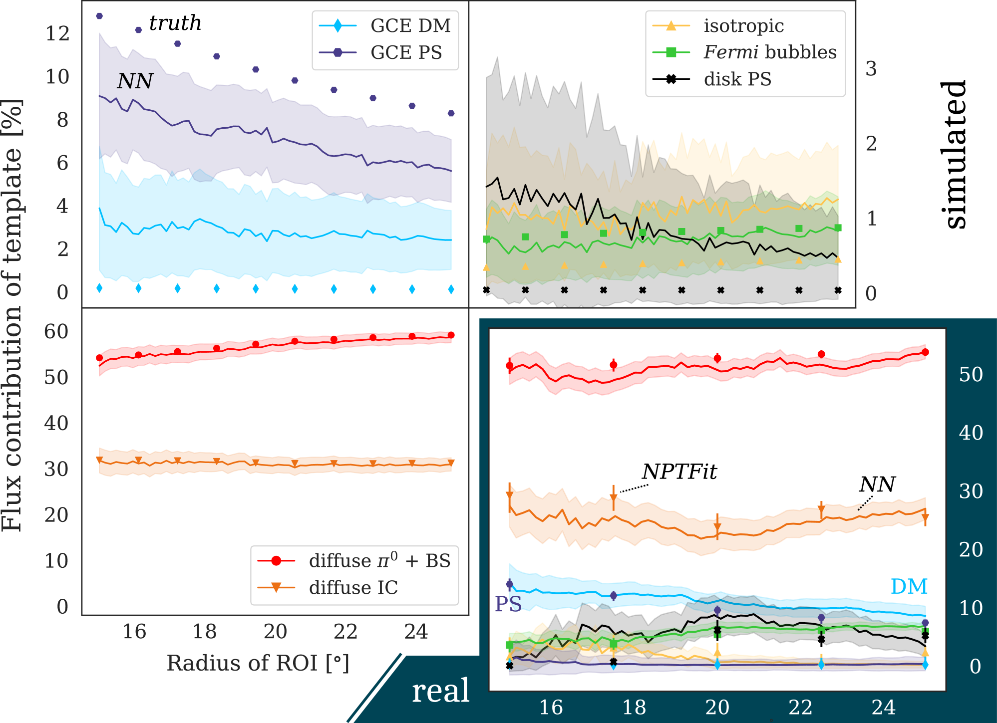
Now, we train a Bayesian GCNN on photon-count maps consisting of all the templates: those used in the proof-of-concept example above, plus the disk PS template. We mask again the inner around the Galactic Plane and train on photon-count maps covering the inner around the GC. Moreover, we mask the resolved 3FGL sources [63] at containment in order for the flux within the ROI not to be dominated by known bright PSs. The training maps account for the non-uniform Fermi exposure. In order to obtain realistic simulated maps, we fit the Fermi data using NPTFit within a ROI (the region that drives the NPTF evidence for GCE PS) and generate 250 mock realizations that correspond to the medians of the model parameter posteriors. For this setting, NPTFit finds a point-like GCE, and the identified GCE DM flux is consistent with zero. In this ROI, the isotropic, bubbles, and disk PS fluxes are negligible (). We apply our NN to each of the 250 mock maps for 64 ROIs, delimited by a radius that monotonically increases in equal steps from to around the GC. Figure 2 (upper left panels) shows the predictions of the NN (solid lines) and the 1 scatter (shaded regions) over the mock samples, as a function of the ROI radius. The fluxes of the non-GCE templates are accurately predicted, but a fraction of the GCE PS flux is incorrectly attributed to the GCE DM template. This is a manifestation of the PS-DM degeneracy expected for the simulated PS distribution, and reflective of the dim nature of the GCE PSs preferred by NPTFit. We assess the correlation between the source-count distribution for the GCE PSs and the degree of misattribution between the GCE templates in a dedicated experiment in the SM. Nonetheless, the NN correctly identifies the GCE PS template to be the main constituent of the GCE in of the maps. Further, in all cases the sum of GCE DM and PS contribution is consistent with the GCE flux injected, indicating the absence of confusion with additional templates such as the disk PSs that were absent in our proof-of-concept tests. In the SM, we consider the same experiment for mock maps corresponding to the NPTF best-fit parameters determined using a larger ROI radius of with higher disk and bubble fluxes, which the NN correctly detects.
In Fig. 2 (lower right), we plot the predictions of the NN for the real Fermi data, evaluated in the same 64 ROIs, together with those of NPTFit for 5 ROIs. Now, the shaded regions indicate the predictive uncertainties of the NN (aleatoric and epistemic added in quadrature). While the NN predictions for the diffuse templates resemble those for the mock data, the GCE flux is almost entirely attributed to annihilating DM, with GCE PS being consistent with zero flux. As expected, the predicted GCE DM contribution decreases as the ROI is enlarged. The credible intervals are similar in size to the scatter of the NN predictions over the mock samples, decreasing in general as the ROI radius increases (more pixels are at the disposal of the NN), and are smaller for templates that are easy for the NN to predict thanks to their distinct shape such as the Fermi bubbles. In the SM, we show that the estimated uncertainties are generally larger for maps and templates where the NN estimates are less accurate and vice versa. The flux contributions and in particular the total GCE flux predicted by NPTFit and the NN mostly agree with each other, with the exception of the GCE flux being ascribed to DM by the NN instead of PS: the NN / NPTFit predictions for the GCE templates within are (in ): / (GCE DM) and / (GCE PS), respectively, while the predictions for the other templates are / (diffuse ), / (diffuse IC), / (isotropic), / (Fermi bubbles), and / (disk PS). This preference for GCE DM over GCE PS persists for three additional diffuse models and when replacing the thin disk PS template by a thick disk PS template. Yet we also find that the NN can underestimate the flux associated with additional GCE PSs injected directly into the data, particularly if they are peaked near the 1 threshold, suggesting if such sources are present their flux is likely underestimated. Accordingly, we refrain from interpreting these results as a definitive statement on the origin of the GCE. A detailed discussion of these points is presented in the SM.
With this work, we establish Bayesian Deep Learning as a powerful tool for disentangling the GCE into its individual components. It is suggestive that our NN identifies a GCE with smooth origin in all our experiments. Nonetheless, as with the NPTF, it will be crucial to further substantiate the robustness of Deep Learning methods to systematics such as diffuse mismodeling and the DM density profile. We present several encouraging results in the presence of either of these two mismodeling sources in the SM. In addition to new measurements and improved diffuse emission models, Deep Learning has the potential to critically contribute to the unraveling of the GCE mystery within the coming years.
Acknowledgements.
Our work benefited from the feedback of Mariangela Lisanti, Ben Safdi, and Tracy Slatyer. The authors acknowledge the National Computational Infrastructure (NCI), which is supported by the Australian Government, for providing services and computational resources on the supercomputer Gadi that have contributed to the research results reported within this paper. We further acknowledge the technical assistance provided by the Sydney Informatics Hub, a Core Research Facility of the University of Sydney, and the generous allocation of resources through the Computational Grand Challenge program. The authors thank the Fermi collaboration for making the data publicly available. FL is supported by the University of Sydney International Scholarship (USydIS). NLR is supported by the Miller Institute for Basic Research in Science at the University of California, Berkeley. This work made use of the free Python packages matplotlib [64], seaborn [65], numpy [66], scipy [67], healpy [68], Tensorflow [59], ray [69], NPTFit [34], NPTFit-Sim [49], dill [70], and cloudpickle.333https://github.com/cloudpipe/cloudpickle Also, we intensively used the arXiv preprint repository and the free software Inkscape.444https://inkscape.org/References
- Bertone et al. [2005] G. Bertone, D. Hooper, and J. Silk, Phys. Rep. 405, 279 (2005), arXiv:0404175 [hep-ph] .
- Goodenough and Hooper [2009] L. Goodenough and D. Hooper, (2009), arXiv:0910.2998 [hep-ph] .
- Hooper and Goodenough [2011] D. Hooper and L. Goodenough, Phys. Lett. B 697, 412 (2011), arXiv:1010.2752 [hep-ph] .
- Hooper and Linden [2011] D. Hooper and T. Linden, Phys.Rev. D84, 123005 (2011), arXiv:1110.0006 [astro-ph.HE] .
- Abazajian and Kaplinghat [2012] K. N. Abazajian and M. Kaplinghat, Phys. Rev. D 86, 083511 (2012), [Erratum: Phys.Rev.D 87, 129902 (2013)], arXiv:1207.6047 [astro-ph.HE] .
- Hooper and Slatyer [2013] D. Hooper and T. R. Slatyer, Phys. Dark Univ. 2, 118 (2013), arXiv:1302.6589 [astro-ph.HE] .
- Gordon and Macias [2013] C. Gordon and O. Macias, Phys.Rev. D88, 083521 (2013), arXiv:1306.5725 [astro-ph.HE] .
- Abazajian et al. [2014] K. N. Abazajian, N. Canac, S. Horiuchi, and M. Kaplinghat, Phys. Rev. D 90, 023526 (2014), arXiv:1402.4090 .
- Daylan et al. [2016] T. Daylan, D. P. Finkbeiner, D. Hooper, T. Linden, S. K. Portillo, N. L. Rodd, and T. R. Slatyer, Phys. Dark Univ. 12, 1 (2016), arXiv:1402.6703 .
- Calore et al. [2015] F. Calore, I. Cholis, and C. Weniger, JCAP 2015 (03), 038, arXiv:1409.0042 .
- Abazajian et al. [2015] K. N. Abazajian, N. Canac, S. Horiuchi, M. Kaplinghat, and A. Kwa, JCAP 1507 (07), 013, arXiv:1410.6168 [astro-ph.HE] .
- Ajello et al. [2016] M. Ajello, A. Albert, W. B. Atwood, G. Barbiellini, D. Bastieri, K. Bechtol, R. Bellazzini, E. Bissaldi, et al., ApJ 819, 44 (2016), arXiv:1511.02938 .
- Linden et al. [2016] T. Linden, N. L. Rodd, B. R. Safdi, and T. R. Slatyer, Phys. Rev. D 94, 103013 (2016), arXiv:1604.01026 .
- Macias et al. [2018] O. Macias, C. Gordon, R. M. Crocker, B. Coleman, D. Paterson, S. Horiuchi, and M. Pohl, Nat. Astron. 2, 387 (2018), arXiv:1611.06644 [astro-ph.HE] .
- Clark et al. [2018] H. A. Clark, P. Scott, R. Trotta, and G. F. Lewis, JCAP 2018 (07), 060.
- Mirabal [2013] N. Mirabal, MNRAS 436, 2461 (2013).
- Petrović et al. [2015] J. Petrović, P. D. Serpico, and G. Zaharijas, JCAP 1502 (02), 023, arXiv:1411.2980 [astro-ph.HE] .
- Yuan and Ioka [2015] Q. Yuan and K. Ioka, Astrophys. J. 802, 124 (2015), arXiv:1411.4363 [astro-ph.HE] .
- O’Leary et al. [2015] R. M. O’Leary, M. D. Kistler, M. Kerr, and J. Dexter, (2015), arXiv:1504.02477 .
- Brandt and Kocsis [2015] T. D. Brandt and B. Kocsis, Astrophys. J. 812, 15 (2015), arXiv:1507.05616 [astro-ph.HE] .
- Carlson and Profumo [2014] E. Carlson and S. Profumo, Phys. Rev. D 90, 023015 (2014), arXiv:1405.7685 .
- Petrović et al. [2014] J. Petrović, P. D. Serpico, and G. Zaharijaš, JCAP 2014 (10), 052.
- Cholis et al. [2015] I. Cholis, C. Evoli, F. Calore, T. Linden, C. Weniger, and D. Hooper, JCAP 2015 (12), arXiv:1506.05119 .
- Ploeg et al. [2017] H. Ploeg, C. Gordon, R. Crocker, and O. Macias, JCAP 2017 (08), 015, arXiv:1705.00806 .
- Bartels et al. [2018a] R. Bartels, E. Storm, C. Weniger, and F. Calore, Nat. Astron. 2, 819 (2018a), arXiv:1711.04778 [astro-ph.HE] .
- Macias et al. [2019] O. Macias, S. Horiuchi, M. Kaplinghat, C. Gordon, R. M. Crocker, and D. M. Nataf, JCAP 09, 042, arXiv:1901.03822 [astro-ph.HE] .
- Abazajian et al. [2020] K. N. Abazajian, S. Horiuchi, M. Kaplinghat, R. E. Keeley, and O. Macias, (2020), arXiv:2003.10416 .
- Bartels et al. [2016] R. Bartels, S. Krishnamurthy, and C. Weniger, Phys. Rev. Lett. 116, 051102 (2016).
- McDermott et al. [2016] S. D. McDermott, P. J. Fox, I. Cholis, and S. K. Lee, JCAP 2016 (07), 045.
- Balaji et al. [2018] B. Balaji, I. Cholis, P. J. Fox, and S. D. McDermott, Phys. Rev. D 98, 043009 (2018).
- Malyshev and Hogg [2011] D. Malyshev and D. W. Hogg, Astrophys. J. 738, 181 (2011), arXiv:1104.0010 [astro-ph.CO] .
- Lee et al. [2015] S. K. Lee, M. Lisanti, and B. R. Safdi, JCAP 1505 (05), 056, arXiv:1412.6099 [astro-ph.CO] .
- Lee et al. [2016] S. K. Lee, M. Lisanti, B. R. Safdi, T. R. Slatyer, and W. Xue, Phys. Rev. Lett. 116, 051103 (2016).
- Mishra-Sharma et al. [2017] S. Mishra-Sharma, N. L. Rodd, and B. R. Safdi, The Astronomical Journal 153, 253 (2017), arXiv:1612.03173 .
- Zhong et al. [2019] Y.-M. Zhong, S. D. McDermott, I. Cholis, and P. J. Fox, (2019), arXiv:1911.12369 [astro-ph.HE] .
- Buschmann et al. [2020] M. Buschmann, N. L. Rodd, B. R. Safdi, L. J. Chang, S. Mishra-Sharma, M. Lisanti, and O. Macias, (2020), arXiv:2002.12373 .
- Leane and Slatyer [2020a] R. K. Leane and T. R. Slatyer, (2020a), arXiv:2002.12370 .
- Leane and Slatyer [2020b] R. K. Leane and T. R. Slatyer, (2020b), arXiv:2002.12371 .
- Leane and Slatyer [2019a] R. K. Leane and T. R. Slatyer, Phys. Rev. Lett. 123, 241101 (2019a).
- Chang et al. [2020] L. J. Chang, S. Mishra-Sharma, M. Lisanti, M. Buschmann, N. L. Rodd, and B. R. Safdi, Phys. Rev. D 101, 023014 (2020), arXiv:1908.10874 .
- Gorski et al. [2005] K. M. Gorski, E. Hivon, A. J. Banday, B. D. Wandelt, F. K. Hansen, M. Reinecke, and M. Bartelmann, ApJ 622, 759 (2005), arXiv:0409513 [astro-ph] .
- Perraudin et al. [2019] N. Perraudin, M. Defferrard, T. Kacprzak, and R. Sgier, Astronomy and Computing 27, 130 (2019), arXiv:1810.12186 .
- Defferrard et al. [2020] M. Defferrard, M. Milani, F. Gusset, and N. Perraudin, in International Conference on Learning Representations (2020).
- Kendall and Gal [2017] A. Kendall and Y. Gal, Advances in Neural Information Processing Systems 2017-Decem, 5575 (2017), arXiv:1703.04977 .
- Caron et al. [2018] S. Caron, G. A. Gómez-Vargas, L. Hendriks, and R. R. de Austri, JCAP 2018 (05), 058, arXiv:1708.06706 .
- Leane and Slatyer [2019b] R. K. Leane and T. R. Slatyer, (2019b), arXiv:1904.08430 .
- Su et al. [2010] M. Su, T. R. Slatyer, and D. P. Finkbeiner, ApJ 724, 1044 (2010), arXiv:1005.5480 .
- Navarro et al. [1997] J. F. Navarro, C. S. Frenk, and S. D. M. White, ApJ 490, 493 (1997).
- [49] N. Rodd and M. Toomey, NPTFit-Sim.
- Lecun et al. [1998] Y. Lecun, L. Bottou, Y. Bengio, and P. Haffner, Proceedings of the IEEE 86, 2278 (1998).
- Perreault Levasseur et al. [2017] L. Perreault Levasseur, Y. D. Hezaveh, and R. H. Wechsler, ApJ 850, L7 (2017), arXiv:1708.08843 .
- Hortua et al. [2019] H. J. Hortua, R. Volpi, D. Marinelli, and L. Malagò, (2019), arXiv:1911.08508 .
- Petroff et al. [2020] M. A. Petroff, G. E. Addison, C. L. Bennett, and J. L. Weiland, (2020), arXiv:2004.11507 .
- Gal and Ghahramani [2016] Y. Gal and Z. Ghahramani, 33rd International Conference on Machine Learning, ICML 2016 3, 1651 (2016), arXiv:1506.02142 .
- Gal et al. [2017] Y. Gal, J. Hron, and A. Kendall, Advances in Neural Information Processing Systems 2017-Decem, 3582 (2017), arXiv:1705.07832 .
- Hinton et al. [2012] G. E. Hinton, N. Srivastava, A. Krizhevsky, I. Sutskever, and R. R. Salakhutdinov, (2012), arXiv:1207.0580 .
- Srivastava et al. [2014] N. Srivastava, G. Hinton, A. Krizhevsky, I. Sutskever, and R. Salakhutdinov, The journal of machine learning research 15, 1929 (2014).
- Ioffe and Szegedy [2015] S. Ioffe and C. Szegedy, International Conference on Machine Learning , 448 (2015), arXiv:1502.03167 .
- Abadi et al. [2016] M. Abadi, A. Agarwal, P. Barham, E. Brevdo, Z. Chen, C. Citro, G. S. Corrado, A. Davis, et al., (2016), arXiv:1603.04467 .
- Kingma and Ba [2014] D. P. Kingma and J. Ba, (2014), arXiv:1412.6980 .
- Feroz et al. [2009] F. Feroz, M. P. Hobson, and M. Bridges, MNRAS 398, 1601 (2009), arXiv:0809.3437 .
- Buchner et al. [2014] J. Buchner, A. Georgakakis, K. Nandra, L. Hsu, C. Rangel, M. Brightman, A. Merloni, M. Salvato, et al., A&A 564, A125 (2014), arXiv:1402.0004 .
- Acero et al. [2015] F. Acero, M. Ackermann, M. Ajello, A. Albert, W. B. Atwood, M. Axelsson, L. Baldini, J. Ballet, et al., ApJ Supplement Series 218, 23 (2015), arXiv:1501.02003 .
- Hunter [2007] J. D. Hunter, Computing in Science & Engineering 9, 90 (2007).
- Waskom et al. [2017] M. Waskom et al., mwaskom/seaborn: v0.8.1 (september 2017) (2017).
- Oliphant [2006] T. E. Oliphant, A guide to NumPy, Vol. 1 (Trelgol Publishing USA, 2006).
- Virtanen et al. [2020] P. Virtanen et al., Nature Methods https://doi.org/10.1038/s41592-019-0686-2 (2020).
- Zonca et al. [2019] A. Zonca, L. Singer, D. Lenz, M. Reinecke, C. Rosset, E. Hivon, and K. Gorski, Journal of Open Source Software 4, 1298 (2019).
- Moritz et al. [2017] P. Moritz, R. Nishihara, S. Wang, A. Tumanov, R. Liaw, E. Liang, W. Paul, M. I. Jordan, and I. Stoica, CoRR abs/1712.05889 (2017), arXiv:1712.05889 .
- McKerns et al. [2011] M. M. McKerns, L. Strand, T. Sullivan, A. Fang, and M. A. G. Aivazis, Proceedings of the 10th Python in Science Conference (2011).
- Abdollahi et al. [2020] S. Abdollahi, F. Acero, M. Ackermann, M. Ajello, W. B. Atwood, M. Axelsson, L. Baldini, J. Ballet, et al., ApJ Supplement Series 247, 33 (2020), arXiv:1902.10045v6 .
- Ackermann et al. [2012] M. Ackermann, M. Ajello, W. B. Atwood, L. Baldini, J. Ballet, G. Barbiellini, D. Bastieri, K. Bechtol, et al., ApJ 750, 3 (2012), arXiv:1202.4039 .
- Bartels et al. [2018b] R. T. Bartels, T. D. P. Edwards, and C. Weniger, MNRAS 481, 3966 (2018b), arXiv:1805.11097 .
- Cholis et al. [2014] I. Cholis, D. Hooper, and T. Linden, (2014), arXiv:1407.5583 .
- Zechlin et al. [2016] H.-S. Zechlin, A. Cuoco, F. Donato, N. Fornengo, and M. Regis, ApJ 826, L31 (2016), arXiv:1605.04256 .
- Ploeg et al. [2020] H. Ploeg, C. Gordon, R. Crocker, and O. Macias, (2020), arXiv:2008.10821 .
- Bordoloi et al. [2017] R. Bordoloi, A. J. Fox, F. J. Lockman, B. P. Wakker, E. B. Jenkins, B. D. Savage, S. Hernandez, J. Tumlinson, et al., ApJ 834, 191 (2017), arXiv:1612.01578 .
- Lorimer et al. [2006] D. R. Lorimer, A. J. Faulkner, A. G. Lyne, R. N. Manchester, M. Kramer, M. A. McLaughlin, G. Hobbs, A. Possenti, et al., MNRAS 372, 777 (2006).
- Zhang and Guo [2020] R. Zhang and F. Guo, ApJ 894, 117 (2020), arXiv:2003.03625 .
- Platt [1999] J. Platt, Advances in large margin classifiers 10, 61 (1999).
- Kull et al. [2017] M. Kull, T. de Menezes e Silva Filho, and P. Flach, Proceedings of the 20th International Conference on Artificial Intelligence and Statistics, AISTATS 2017 54 (2017).
- Hortúa et al. [2020] H. J. Hortúa, L. Malago, and R. Volpi, Mach. Learn.: Sci. Technol. 1, 035014 (2020), arXiv:2005.07694 .
- Russell and Reale [2019] R. L. Russell and C. Reale, (2019), arXiv:1910.14215 .
- Hinton [2016] S. Hinton, The Journal of Open Source Software 1, 45 (2016).
- Mishra-Sharma and Cranmer [2020] S. Mishra-Sharma and K. Cranmer, (2020), arXiv:2010.10450 .