Temperature dependence of $\eta/s$ of strongly interacting matter: effects of the equation of state and the parametric form of $(\eta/s)(T)$

Abstract

We investigate the temperature dependence of the shear viscosity to entropy density ratio $\eta/s$ using a piecewise linear parametrization. To determine the optimal values of the parameters and the associated uncertainties, we perform a global Bayesian model-to-data comparison on Au+Au collisions at $\sqrt{s_{\mathrm{NN}}}=200$ GeV and Pb+Pb collisions at $2.76$ TeV and $5.02$ TeV, using a 2+1D hydrodynamical model with the EKRT initial state. We provide three new parametrizations of the equation of state (EoS) based on contemporary lattice results and hadron resonance gas, and use them and the widely used $s95p$ parametrization to explore the uncertainty in the analysis due to the choice of the equation of state. We found that $\eta/s$ is most constrained in the temperature range $T\approx 150$–$220$ MeV, where, for all EoSs, $0.08<\eta/s<0.23$ when taking into account the 90% credible intervals. In this temperature range the EoS parametrization has only a small $\approx 10\%$ effect on the favored $\eta/s$ value, which is less than the $\approx 30\%$ uncertainty of the analysis using a single EoS parametrization. Our parametrization of $(\eta/s)(T)$ leads to a slightly larger minimum value of $\eta/s$ than the previously used parametrizations. When we constrain our parametrization to mimic the previously used parametrizations, our favored value is reduced, and the difference becomes statistically insignificant.

I Introduction

The main goal of the ultrarelativistic heavy-ion collisions at the Large Hadron Collider (LHC) and the Relativistic Heavy-Ion Collider (RHIC) is to understand the properties of the strongly interacting matter produced in these collisions. In recent years the main interest has been in extracting the dissipative properties of this QCD matter from the experimental data (e.g. Luzum:2008cw ; Bozek:2009dw ; Song:2011qa ; Ryu:2015vwa ; Karpenko:2015xea ), in particular its specific shear viscosity: the ratio of shear viscosity to entropy density $\eta/s$ (for a review, see Refs. Heinz:2013th ; Gale:2013da ; Huovinen:2013wma ; Shen:2020gef ). The field has matured to a level where a global Bayesian analysis of the parameters can provide statistically meaningful credibility ranges to the temperature dependence of $\eta/s$ Bernhard:2016tnd ; Bass:2017zyn ; Bernhard:2019bmu . These credibility ranges agree with earlier results like those obtained using the EKRT model Niemi:2015qia .

However, with the exception of papers like Refs. Pratt:2015zsa ; Moreland:2015dvc ; Alba:2017hhe , the equation of state (EoS) is taken as given in the models used to extract the $\eta/s$ ratio from the data. Recent fluid dynamical studies generally use an EoS based on contemporary lattice QCD results, but during the last decade many studies in the literature used the EoS parametrization $s95p$ Huovinen:2009yb . This parametrization is based on by now outdated lattice data Bazavov:2009zn , and recent studies have reported an approximate 60% Alba:2017hhe or 30% increases Schenke:2019ruo in the extracted value of $\eta/s$ when switching from $s95p$ to a contemporary lattice-based EoS. Furthermore, even if the errors of the contemporary lattice QCD calculations overlap, there is still a small tension between the trace anomalies obtained using the HISQ Bazavov:2014pvz ; Bazavov:2017dsy and stout Borsanyi:2013bia ; Borsanyi:2010cj discretization schemes. Consequently the EoSs differ, and if the procedure to extract $\eta/s$ from the data is as sensitive to the details of the EoS as Refs. Alba:2017hhe ; Schenke:2019ruo claim, this tension may lead to additional uncertainties in the $\eta/s$ values extracted from the heavy-ion collision data.

In the previously mentioned Bayesian analysis Bernhard:2016tnd ; Bass:2017zyn , where the EoS is based on contemporary lattice data Bazavov:2014pvz , the temperature dependence of $\eta/s$ was assumed to be monotonously increasing above the QCD transition temperature $T_{c}$. In a Bayesian analysis the slope parameter of such parametrization is always constrained to be non-negative, and limiting the final slope parameter to zero would require extremely strong constraints from the experimental data. Therefore, by construction, the analysis leads to an $\eta/s$ increasing with temperature above $T_{c}$, even if there is no physical reason to exclude a scenario where $\eta/s$ is constant in a broad temperature range above $T_{c}$. A more flexible parametrization, which does not impose such constraints, is thus needed to determine the temperature dependence of $\eta/s$.

In this work we address both the sensitivity of the extracted $\eta/s$ to the EoS used in the model calculation, and the temperature dependence of $\eta/s$ in the vicinity of the QCD transition temperature. We perform a Bayesian analysis of the results of EKRT + hydrodynamics calculations Niemi:2015qia ; Niemi:2015voa , and the data obtained in $\sqrt{s_{\mathrm{NN}}}=200$ GeV Au+Au collisions Adler:2004zn ; Adler:2003cb ; Adams:2004bi , and Pb+Pb collisions at $2.76$ TeV Aamodt:2010cz ; Abelev:2013vea ; Adam:2016izf and $5.02$ TeV Adam:2016izf ; Adam:2015ptt . To study the temperature dependence of $\eta/s$ we use a piecewise linear parametrization in three parts: linearly decreasing and increasing regions at low and high temperatures are connected by a constant-value plateau of variable range. With this parametrization, data favoring a strong temperature dependence will lead to large slopes and a narrow plateau; conversely, an approximately constant $\eta/s$ can be obtained with small slope parameter values and a wide plateau. To explore the sensitivity to the EoS, we use four different parametrizations: the well-known $s95p$ parametrization, and three new parametrizations based on contemporary lattice QCD results. A comparison of the final probability distributions of the parameters will tell whether the most probable parameter values depend on the EoS used, and whether that difference is significant when the overall uncertainty in the fitting procedure is taken into account.

II Equation of state

In lattice QCD the calculation of the equation of state (EoS) usually proceeds through the calculation of the trace anomaly, $\Theta(T)=\epsilon(T)-3p(T)$, where $\epsilon$ and $p$ are energy density and pressure, respectively. Thermodynamical variables are subsequently derived from it using so-called integral method Boyd:1996bx . Therefore we base our EoS parametrizations on the trace anomaly and obtain pressure from the integral

$$\frac{p(T)}{T^{4}}-\frac{p(T_{\rm low})}{T^{4}_{\rm low}}=\int_{T_{\rm low}}^{T}\frac{\mathrm{d}T^{\prime}}{{T^{\prime}}^{5}}\Theta(T^{\prime}).$$ (1)

Once the pressure is known, the energy and entropy densities can be calculated, $\epsilon(T)=\Theta(T)+3p(T)$, and $s(T)=[\epsilon(T)+p(T)]/T$, respectively. To make a construction of chemical freeze-out at $T\approx 150$ MeV temperature possible, we use the hadron resonance gas (HRG) trace anomaly at low temperatures instead of the lattice QCD result. Equally important is that this choice allows for energy and momentum conserving switch from fluid degrees of freedom to particle degrees of freedom without any non-physical discontinuities in temperature and/or flow velocity. Furthermore, it gives us a consistent value for the pressure at $T_{\rm low}$ required for the evaluation of pressure (see Eq. (1)).

As a baseline, we use the $s95p$ parametrization Huovinen:2009yb , where HRG containing hadrons and resonances below $M<2$ GeV mass from the 2004 PDG summary tables Eidelman:2004wy is connected to the parametrized hotQCD data from Ref. Bazavov:2009zn . To explore the effects of various developments during the last decade, we first connect the HRG based on the PDG 2004 particle list Eidelman:2004wy to parametrized contemporary lattice data obtained using the HISQ discretization scheme Bazavov:2014pvz ; Bazavov:2017dsy . The lattice spacing, $a$, is related to the temperature and temporal lattice extent, $N_{t}$, as $a=1/(N_{t}T)$. Since the lattice spacing ($N_{t}$) dependence is small for this action, we use these results at fixed lattice spacing $N_{t}=8,10$ and 12. We name our parametrizations according to the convention used to name $s95p$, and label this parametrization $s87h_{04}$. ’$s87$’ signifies entropy density reaching 87% of its ideal gas value at $T=800$ MeV, the letter ’$h$’ refers to the HISQ action, and the subscript ’04’ to the vintage of the PDG particle list (2004). Note that even if our parametrization differs from the lattice trace anomaly in the hadronic phase, it agrees with the contemporary lattice calculations which show that at $T=800$ MeV the entropy density reaches $87$–$88\%$ of the ideal gas value (c.f. Fig. 8 of Ref. Bazavov:2017dsy ).

The number of well-established resonances has increased since 2004, so we base our parametrization $s88h_{18}$ on HRG containing all strange and non-strange hadrons and resonances in the PDG 2018 summary tablesTanabashi:2018oca , and on the same HISQ lattice data Bazavov:2014pvz ; Bazavov:2017dsy we used for $s87h_{04}$. Furthermore, there is a slight tension in the trace anomaly between the HISQ and stout discretization schemes. To explore whether this difference has any effect on hydrodynamical modeling, we construct the parametrization $s83s_{18}$ using PDG 2018 resonances, and the continuum extrapolated lattice data obtained using the stout discretization Borsanyi:2013bia ; Borsanyi:2010cj . The second letter ’$s$’ in the label refers now to the stout action, and the subscript ’18’ to the vintage of the particle list. The details of these parametrizations are shown in Appendix A.

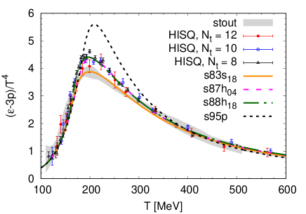
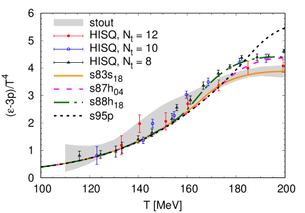
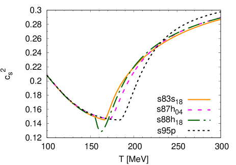
Figure 1: The trace anomaly (top and middle) and the speed of sound squared (bottom) as functions of temperature in the four parametrizations of the EoS compared to the lattice data obtained using the HISQ Bazavov:2014pvz ; Bazavov:2017dsy and stout Borsanyi:2013bia ; Borsanyi:2010cj discretization schemes.

In the top and middle panels of Fig. 1, we show the parametrized trace anomalies, and the lattice data as used to make them: continuum extrapolated for the stout action, and at fixed lattice spacing for the HISQ action, since its lattice spacing ($N_{t}$) dependence is small. As seen in the topmost panel, the most noticable change in the lattice results during the last decade is the reduction of the peak of the trace anomaly (cf. $s95p$ to others). Also, as mentioned, the lattice results obtained using the HISQ and stout actions slightly differ around the peak, and consequently $s83s_{18}$ differs from $s87h_{04}$ and $s88h_{18}$. The higher peak does not, however, mean a lower speed of sound. As shown in the lowest panel of Fig. 1, the speed of sound in the $s95p$ parametrization is not significantly lower than in the other parametrizations, but the temperature region where it is low is broader than in the other parametrizations. Thus we expect $s95p$ to be effectively softer than the other EoSs. On the other hand, the speed of sound in $s88h_{18}$ depicts a characteristic dip below the speed of sound in the other parametrizations. This is a consequence of the parametrization of the trace anomaly in that temperature region.

As known, the HRG trace anomaly is below the lattice results Borsanyi:2010cj ; Borsanyi:2013bia ; Bazavov:2014pvz at low temperatures. This difference has been interpreted to indicate the existence of yet unobserved resonance states Majumder:2010ik ; Huovinen:2018ziu . The need for further states has also been seen in the study of the strangeness baryon correlations on the lattice Bazavov:2014xya , and confirmed by the S-matrix based virial expansion Fernandez-Ramirez:2018vzu . However, we do not include predicted states from any model in this work, since we do not know how they would decay, but use the states from the PDG summary tables only. Consequently the parametrized trace anomaly is slightly below even the most generous error bars of the lattice results around $T\approx 150$–160 MeV temperature, as shown in the middle panel of Fig. 1.

On the other hand, whether we use the PDG 2004 or 2018 particle list causes only a tiny difference in the trace anomaly. The main difference between the $s87h_{04}$ and $s88h_{18}$ parametrizations arises from the connection of the HRG to the lattice parametrization. When parametrizing $s88h_{18}$ we wanted the trace anomaly to reach its lattice values soon above $T_{c}=155$ MeV, whereas we allowed $s87h_{04}$ to agree with lattice at larger temperature where the lattice trace anomaly drops below the HRG trace anomaly—for details, see Appendix A. Consequently the $s88h_{18}$ parametrization rises above the HRG values leading to the characteristic dip in the speed of sound (lowest panel in Fig. 1). Note that the $s83s_{18}$ parametrization does not depict a similar dip in the speed of sound, since the lower peak and larger errors of the continuum extrapolated stout action result allow the parametrized trace anomaly to drop below the HRG values immediately.

III Hydrodynamical model

We employ a fluid dynamical model used previously in Refs. Niemi:2012ry ; Niemi:2011ix ; Niemi:2015qia ; Niemi:2015voa ; Eskola:2017bup . The spacetime evolution is computed numerically in (2+1) dimensions Molnar:2009tx , and the longitudinal expansion is accounted for by assuming longitudinal boost invariance. We also neglect here the bulk viscosity and the small net-baryon number. The evolution of the shear-stress tensor $\pi^{\mu\nu}$ is described by the second-order Israel-Stewart formalism Israel:1979wp , with the coefficients of the non-linear second-order terms obtained by using the 14-moment approximation in the ultrarelativistic limit Denicol:2012cn ; Molnar:2013lta . The shear relaxation time is related to the shear viscosity by $\tau_{\pi}=5\eta/(\epsilon+p)$, where $\epsilon$ is energy density in the local rest frame, and $p$ is thermodynamic pressure.

Transverse momentum spectra of hadrons are computed by using the Cooper-Frye freeze-out formalism at a constant-temperature surface, followed by all 2- and 3-body decays of unstable hadrons. The chemical freeze-out is encoded into the EoS as described in Ref. Huovinen:2007xh , and the fluid evolves from chemical to kinetic freeze-out in partial chemical equilibrium (PCE)Hirano:2002ds . The kinetic and chemical freeze-out temperatures $T_{\mathrm{dec}}$ and $T_{\mathrm{chem}}$ are left as free parameters to be determined from the experimental data through the Bayesian analysis. The dissipative corrections $\delta f$ to the momentum distribution at the freeze-out are computed according to the usual 14-moment approximation $\delta f_{\mathbf{k}}\propto f_{0\mathbf{k}}k^{\mu}k^{\nu}\pi_{\mu\nu}$, where $f_{0\mathbf{k}}$ is the equilibrium distribution function, and $k^{\mu}$ is the four-momentum of the hadron.

The remaining input to fluid dynamics are the EoS, initial conditions, and the shear viscosity. The different options for EoS were discussed in the previous section, and the initial conditions will be detailed in the next section. The temperature dependence of the shear viscosity $\eta/s$ is parametrized in three parts, controlled by $T_{\mathrm{H}}$, the lower bound of the temperature range where $\eta/s$ has its minimum value, $(\eta/s)_{\mathrm{min}}$, and the width of this temperature range, $W_{\mathrm{min}}$:

$$(\eta/s)(T)=\begin{cases}S_{\mathrm{HG}}(T_{\mathrm{H}}-T)+(\eta/s)_{\mathrm{min}},&T<T_{\mathrm{H}}\\ (\eta/s)_{\mathrm{min}},&\!\!\!\!\!\!\!\!\!\!\!\!\!\!\!T_{\mathrm{H}}\leq T\leq T_{\rm Q}\\ S_{\mathrm{QGP}}(T-T_{\rm Q})+(\eta/s)_{\mathrm{min}},&T>T_{\rm Q},\end{cases}$$ (2)

where the additional parameters are the linear slopes below $T_{\mathrm{H}}$ and above $T_{\rm Q}=T_{\mathrm{H}}+W_{\mathrm{min}}$, denoted by $S_{\mathrm{HG}}$ and $S_{\mathrm{QGP}}$, respectively.

We note that bulk viscosity and chemical non-equilibrium are related Paech:2006st ; Dusling:2011fd . Even if we ignore the bulk viscosity, some of its effects are accounted for by the fugacities in a chemically frozen fluid: At temperatures below $T_{\mathrm{chem}}$ the isotropic pressure is reduced compared to the equilibrium pressure due to the different chemical composition. Thus introducing the chemical freeze-out changes not only the particle yields w.r.t. evolution in equilibrium, but similarly to the bulk viscosity, reduces the average transverse momentum of hadrons too. However, this affects the evolution only when temperature is below $T_{\mathrm{chem}}$, and in contrast to the bulk viscosity, there is e.g. no entropy production associated with the chemical freeze-out and subsequent chemical non-equilibrium Bebie:1991ij .

Finally, we emphasize that we solve the spacetime evolution from the hot QGP all the way to the kinetic freeze-out as a single continuous fluid dynamical evolution. This is different from the hybrid models used e.g. in Refs. Bernhard:2016tnd ; Bass:2017zyn ; Bernhard:2019bmu where the evolution below some switching temperature is solved with a microscopic hadron cascade. The advantage of the fluid dynamical evolution without a cascade stage is that the transport properties are continuous in the whole temperature range. Note that in the hybrid models the switching from fluid dynamics to hadron cascade introduces an unphysical discontinuity in e.g. $\eta/s$ that is $\mathcal{O}(1)$ in the cascade Rose:2017bjz , but $\mathcal{O}(0.1)$ in fluid dynamical simulations at switching. Another advantage of our approach is that we can freely parametrize the viscosity in the hadronic matter too, and constrain it using the experimental data.

IV Initial conditions

The initial energy density profiles are determined using the EKRT model Eskola:1999fc ; Paatelainen:2012at ; Paatelainen:2013eea based on the NLO perturbative QCD computation of the transverse energy, and a gluon saturation conjecture. The latter controls the transverse energy production through a local semi-hard scale $p_{\rm sat}(T_{A}T_{A},\sqrt{s_{\mathrm{NN}}},A,K_{\rm sat})$, where $T_{A}(x,y)$ is a nuclear thickness function at transverse location $(x,y)$. The essential free parameters in the EKRT model are the proportionality constant $K_{\rm sat}$ in the saturation condition, and the constant $\beta$ controlling the exact definition of the minijet transverse energy at NLO Paatelainen:2012at . The setup used here is identical to the one used in Refs. Niemi:2015qia ; Niemi:2015voa ; Eskola:2017bup , where $\beta=0.8$, and $K_{\rm sat}$ is left as a free parameter to be determined from the data. We note that $K_{\rm sat}$ is independent of the collision energy $\sqrt{s_{\rm NN}}$ and nuclear mass number $A$, so that once $K_{\rm sat}$ is fixed the $\sqrt{s_{\rm NN}}$ and $A$ dependence of the initial conditions is entirely determined from the QCD dynamics of the EKRT model. With a given $p_{\rm sat}$ the local energy density at the formation time $\tau_{p}=1/p_{\rm sat}$ can be written as

$$\epsilon(x,y,\tau_{p})=\frac{K_{\mathrm{sat}}}{\pi}\left[p_{\rm sat}(x,y)\right]^{4}.$$ (3)

This we further evolve to the same proper time $\tau_{0}=1/p_{\rm min}$, where $p_{\rm min}=1$ GeV, at every point in the transverse plane where $p_{\rm sat}>p_{\rm min}$ by using 0+1 dimensional Bjorken hydrodynamics with the assumption $\epsilon=3p$.

In the EKRT model, fluctuations in the product of the nuclear thickness functions, $T_{A}T_{A}$, give rise to the event-by-event fluctuations in the energy density through $p_{\rm sat}$ in Eq. (3). Moreover, the centrality dependence of the initial conditions arises from the centrality dependence of $T_{A}T_{A}$. A full treatment of the dynamics in heavy-ion collisions would take the event-by-event fluctuations into account by evolving each event separately. However, to make the present study computationally feasible, we omit the evolution of such fluctuations here; instead, for each centrality class, we average a large number of these fluctuating initial states, and compute the fluid dynamical evolution only for the averaged initial distributions.

The computed energy densities are not linear in $K_{\rm sat}$ nor in $T_{A}T_{A}$, and different averaging procedures can lead to significantly different event-averaged initial conditions. In the previous event-by-event EKRT studies Niemi:2015qia ; Niemi:2015voa ; Eskola:2017bup a fair agreement was obtained between the data and the computed $\sqrt{s_{\rm NN}}$, $A$, and centrality dependencies of the charged hadron multiplicity. To preserve as much as possible of this agreement, we average the initial conditions by averaging the initial entropy distributions: We compute first a large set of initial energy density profiles using the procedure detailed in Ref. Niemi:2015qia . Each of the generated energy density profiles is converted to an entropy density profile by using the EoS which will be used later during the evolution. The entropy density profiles are then averaged, and the average entropy density profile is converted to an average energy density profile using the same EoS.

In the event-by-event framework the centrality classes were determined from the final multiplicity distribution. However, this way of classifying events is not available here, as it would require fluid dynamical evolution of each of the fluctuating initial conditions. Instead, we pre-determine the centrality classes according to the number of wounded nucleons in the sampled Monte-Carlo nuclear configurations, which were used to construct the event-by-event initial conditions. The number of wounded nucleons are computed using the nucleon-nucleon cross section $\sigma_{\rm NN}=42$, $64$, and $70$ mb for $200$ GeV, $2.76$ TeV, and $5.02$ TeV collisions, respectively. We note that the nucleon-nucleon cross section does not enter in the computation of the initial conditions, but they are used here only in the centrality classification. In the context of the full event-by-event modeling we have tested that the final results are only weakly sensitive to the precise way of the centrality classification.

V Statistical analysis

The eight free parameters of our model, $\{K_{\mathrm{sat}}$, $(\eta/s)_{\mathrm{min}},T_{\mathrm{H}},W_{\mathrm{min}},S_{\mathrm{HG}},S_{\mathrm{QGP}},T_{\mathrm{dec}},T_{\mathrm{chem}}\}$, were introduced in Secs. III and IV. We want to tune them to achieve the best possible fit to an experimental data set of 90 data points. This set consists of the following observables at (10–20)%, (20–30)%, (30–40)%, (40–50)% and (50–60)% centrality classes:

• The charged particle multiplicity at midrapidity, $\mathrm{d}N_{\mathrm{ch}}/\mathrm{d}\eta$, and 4-particle cumulant $p_{T}$-averaged elliptic flow, $v_{2}\{4\}$, in Au+Au collisions at $\sqrt{s_{\mathrm{NN}}}=200$ GeV (RHIC) Adler:2004zn ; Adams:2004bi and Pb+Pb collisions at $\sqrt{s_{\mathrm{NN}}}=2.76$ Aamodt:2010cz ; Adam:2016izf and $\sqrt{s_{\mathrm{NN}}}=5.02$ TeV Adam:2016izf ; Adam:2015ptt (LHC).

• The multiplicities at midrapidity, $\mathrm{d}N_{i}/\mathrm{d}y$, and average transverse momenta $\langle p_{T}\rangle_{i}$, of pions ($\pi^{+}$), kaons ($K^{+}$) and protons ($p$) in Au+Au collisions at RHIC Adler:2003cb and in Pb+Pb collisions at the lower LHC energy Abelev:2013vea .

Let us consider each combination of the free parameters as a point $\vec{x}$ in the 8-dimensional input (parameter) space, the model output $\vec{y}(\vec{x})$ as a corresponding point in the 90-dimensional output space (space of observables), and the experimental data $\vec{y}^{\text{\,exp}}$ as the target point in the space of observables. With these definitions we can formulate the posterior probability distribution $P(\vec{x}|\vec{y}^{\text{\,exp}})$ of the best-fit parameter values by utilizing Bayes’ theorem:

$$P(\vec{x}|\vec{y}^{\text{\,exp}})\propto P(\vec{y}^{\text{\,exp}}|\vec{x})P(\vec{x}),$$ (4)

where $P(\vec{x})$ is the prior probability distribution of input parameters and $P(\vec{y}^{\text{\,exp}}|\vec{x})$ is the likelihood function

$$P(\vec{y}^{\text{\,exp}}|\vec{x})$$

$$= \frac{1}{\sqrt{|2\pi\Sigma|}}\exp\left(-\frac{1}{2}(\vec{y}(\vec{x})-\vec{y}^{\text{\,exp}})^{T}\Sigma^{-1}(\vec{y}(\vec{x})-\vec{y}^{\text{\,exp}})\right).$$

Here $\Sigma$ is the covariance matrix representing the uncertainties related to the model-to-data comparison.

As a function with an eight-dimensional domain, the posterior probability distribution $P(\vec{x}|\vec{y}^{\text{\,exp}})$ is too complicated to evaluate and analyze fully. Instead, we produce samples of it with a parallel tempered Markov chain Monte Carlo Vousden:2016 based on the emcee sampler ForemanMackey:2012ig . An ensemble of random walkers is initialized in the input parameter space based on the prior probability and each proposed step in parameter space is accepted or rejected based on the change in the value of the likelihood function. At a large number of steps, the distribution of the taken steps is expected to converge to the posterior distribution.

Evaluating the output $\vec{y}(\vec{x})$ of the fluid dynamical model at every point $\vec{x}$ where the random walker might enter is a computationally impossible task. Therefore we approximate the output using Gaussian process (GP) emulators Rasmussen:2006 (see Appendix B). Each GP is able to provide estimates for only one observable, so to keep the number of required emulators manageable, we perform a principal component analysis (PCA) to reduce the dimension of the output space from 90 observables into $k=6$ most important principal components. Further details about the PCA are described in Appendix C. We utilize the scikit-learn Python module Pedregosa:2012toh and in particular the submodules sklearn.gaussian_process and sklearn.decomposition.PCA in the model emulation.

Thus, in our likelihood function (V), we replace $\vec{y}(\vec{x})$ with the GP estimate in the principal component space $\vec{z}^{\,\text{GP}}(\vec{x})$ (likewise $\vec{y}^{\text{\,exp}}$ is transformed to $\vec{z}^{\text{\,exp}}$), and include the emulator estimation error into the covariance matrix:

$$\Sigma_{z}=\Sigma_{z}^{\text{exp}}+\Sigma_{z}^{\text{GP}},$$ (6)

where $\Sigma_{z}^{\text{exp}}$ is the (originally diagonal) experimental error matrix transformed to principal component space, and

$$\Sigma_{z}^{\text{GP}}=\text{diag}(\sigma_{z,1}^{\text{GP}}(\vec{x})^{2},\sigma_{z,2}^{\text{GP}}(\vec{x})^{2},...,\sigma_{z,k}^{\text{\,GP}}(\vec{x})^{2})$$ (7)

is the GP emulator covariance matrix obtained from the emulator (see Appendix B).

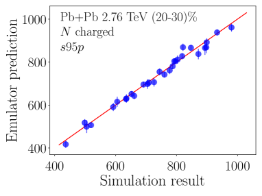
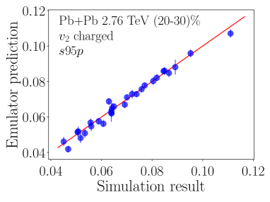
Figure 2: Illustration of the quality of the Gaussian process emulation for 30 test points for simulations with the $s95p$ EoS. Upper panel: Charged particle multiplicity in (20-30)% most central Pb+Pb collisions at $\sqrt{s_{\mathrm{NN}}}=2.76$ TeV. Lower panel: Elliptic flow $v_{2}\{\text{RP}\}$ in (20-30)% most central Pb+Pb collisions at $\sqrt{s_{\mathrm{NN}}}=2.76$ TeV.

To work, the GP emulators must be conditioned with a set of training points, $\{\vec{z}(\vec{x}_{i})\}$, created by running the fluid dynamical model with several different parameter combinations $\{\vec{x}_{i}\}$. For the present investigation, we have produced 170 training points for each EoS, distributed evenly in the input parameter space using minmax Latin hypercube sampling pyDOE:LHS . The emulation quality was then checked by using the trained emulator to predict the results at 30 additional test points, which were not part of the training data. An example of the results of this confirmation process is shown in Fig. 2 for 2.76 TeV Pb+Pb collisions using the $s95p$ parametrization.

VI Results

The marginal posterior probability distributions for each parameter are obtained from the full 8-dimensional probability distribution (see Section V) by integrating over the other seven parameters. The resulting distributions when using the four investigated EoSs are shown in Figs. 3 and 4. In these figures the range of the x-axis illustrates the prior range of values, with the exception of $T_{\mathrm{chem}}$ which range depends on the EoS. The median values of these distributions provide a good approximation for the most probable values, and are listed both in the legends of the figures, and in Table 1. The 90% credible intervals—i.e. the range which covers 90% of the distribution around the median—are shown as errors in Table 1. Two dimensional projections of the probability distribution depicting correlations between parameter pairs are shown in Appendix D.

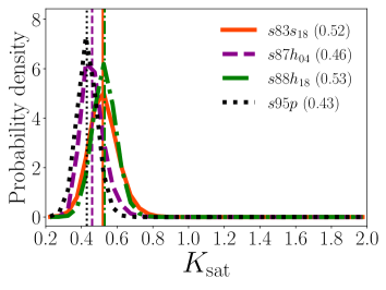
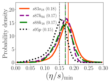
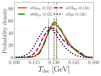
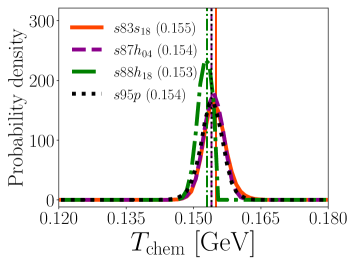
Figure 3: Comparison of $K_{\mathrm{sat}}$, $(\eta/s)_{\mathrm{min}}$, $T_{\mathrm{dec}}$, and $T_{\mathrm{chem}}$ marginal posterior probability distributions for the four investigated EoSs. Vertical lines (bracketed numbers in legend) indicate median values for the distributions. With the exception of $T_{\mathrm{chem}}$, the range of the x-axis in the plots is the original prior range.

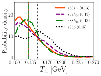
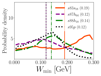
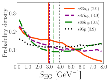
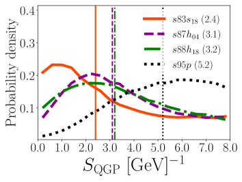
Figure 4: As Fig. 3, but showing the marginal posterior probability distributions of $T_{\mathrm{H}}$, $W_{\mathrm{min}}$, $S_{\mathrm{HG}}$, and $S_{\mathrm{QGP}}$.

VI.1 Nuisance parameters

The analysis involves three parameters which are not directly related to the transport properties of produced matter: $K_{\mathrm{sat}}$, $T_{\mathrm{dec}}$, and $T_{\mathrm{chem}}$. The probability distributions for these three ”nuisance” parameters, shown in Fig. 3, are nicely peaked, and the parameters have well defined constraints. For the chemical freeze-out temperature, the median is $T_{\mathrm{chem}}=153$–$155$ MeV, which is compatible with the values obtained using the statistical hadronization model Andronic:2017pug . Note that the difference in the median is not due to the resonance content of the EoS, but due to a complicated interplay of the softness of the EoS, shear, and build-up of the flow. Nevertheless, the particle ratios are the dominant factor in constraining $T_{\mathrm{chem}}$.

For $K_{\mathrm{sat}}$ and $T_{\mathrm{dec}}$, we see a common trend where $s95p$ gives a distribution which peaks at the lowest value of the four EoSs, followed by $s87h_{04}$, and the highest peak values are shared by $s83s_{18}$ and $s88h_{18}$ with almost identical distributions. The obtained values for the EKRT normalization parameter, $K_{\mathrm{sat}}\approx 0.5$, are compatible with the values found previously Niemi:2015qia , and the small differences between different EoS parametrizations result from slightly different entropy production during the evolution. Differences seen in the kinetic freeze-out temperature $T_{\mathrm{dec}}=126$–$132$ MeV are also small, and seem to follow the conventional rule of thumb: a softer EoS requires a lower freeze-out temperature to create hard enough proton $p_{\mathrm{T}}$ distributions. On the other hand, differences in the median values of all these three parameters are smaller than the credibility intervals, and thus not statistically meaningful.

Table 1: Estimated parameter values (medians) and uncertainties (90% credible intervals) from the posterior distributions.

Parameter		$s83s_{18}$		$s87h_{04}$		$s88h_{18}$		$s95p$
$K_{\mathrm{sat}}$		$0.52$	${}^{+0.15}_{-0.12}$	$0.46$	${}^{+0.12}_{-0.09}$	$0.53$	${}^{+0.11}_{-0.10}$	$0.43$	${}^{+0.10}_{-0.09}$
$(\eta/s)_{\mathrm{min}}$		$0.18$	${}^{+0.04}_{-0.06}$	$0.17$	${}^{+0.03}_{-0.07}$	$0.17$	${}^{+0.04}_{-0.06}$	$0.15$	${}^{+0.03}_{-0.07}$
$T_{H}$	[GeV]	$0.13$	${}^{+0.05}_{-0.03}$	$0.13$	${}^{+0.06}_{-0.03}$	$0.13$	${}^{+0.06}_{-0.03}$	$0.15$	${}^{+0.06}_{-0.04}$
$W_{\mathrm{min}}$	[GeV]	$0.19$	${}^{+0.10}_{-0.17}$	$0.12$	${}^{+0.15}_{-0.11}$	$0.14$	${}^{+0.13}_{-0.12}$	$0.12$	${}^{+0.10}_{-0.10}$
$S_{\mathrm{HG}}$	[GeV-1]	$2.9$	${}^{+4.0}_{-2.7}$	$3.0$	${}^{+4.5}_{-2.8}$	$3.4$	${}^{+4.2}_{-3.2}$	$3.9$	${}^{+3.7}_{-3.6}$
$S_{\mathrm{QGP}}$	[GeV-1]	$2.4$	${}^{+4.9}_{-2.1}$	$3.1$	${}^{+4.2}_{-2.5}$	$3.2$	${}^{+4.1}_{-2.7}$	$5.2$	${}^{+2.5}_{-3.5}$
$T_{\mathrm{dec}}$	[MeV]	$132$	${}^{+14}_{-11}$	$130$	${}^{+16}_{-12}$	$132$	${}^{+15}_{-10}$	$126$	${}^{+15}_{-12}$
$T_{\mathrm{chem}}$	[MeV]	$155$	${}^{+4}_{-4}$	$154$	${}^{+4}_{-3}$	$153$	${}^{+2}_{-3}$	$154$	${}^{+4}_{-4}$

VI.2 $(\eta/s)(T)$

At first sight $(\eta/s)_{\mathrm{min}}$ depicts the behavior described in Refs. Alba:2017hhe ; Schenke:2019ruo : the favored value is lower for $s95p$ than for the newer parametrizations (see Fig. 3 and Table 1). However, the effect is noticeably smaller than seen in those studies—only $\approx 10$–$20\%$—and well within the 90% credible intervals ($\pm\approx 30\%$) of the analysis. The comparison of $\eta/s$ for different EoSs is further complicated by the large number of parameters controlling the temperature dependence of $\eta/s$. The probability distributions of parameters $T_{\mathrm{H}},W_{\mathrm{min}},S_{\mathrm{HG}},$ and $S_{\mathrm{QGP}}$, shown in Fig. 4, are very broad extending to the whole prior range in most cases, and thus do not possess any clearly favored values. However, the wide posterior distributions of the $(\eta/s)(T)$ parameters are partly caused by the inherent ambiguity in the chosen parametrization: for a given temperature $T$, multiple parameter combinations can generate similar values of $\eta/s$. For example, at low temperatures $(\eta/s)(T)$ is mostly determined by $S_{\mathrm{HG}}$ and $T_{\mathrm{H}}$, but it is better constrained than either of these parameters. The reason is that $S_{\mathrm{HG}}$ and $T_{\mathrm{H}}$ are not independent, but slightly anti-correlated—the correlations between the pairs of parameters are shown in Appendix D. Thus it is more illustrative to construct the probability distribution for $\eta/s$ values w.r.t. temperature, and plot the median and credibility intervals of this distribution as shown in Figs. 5 and 6.

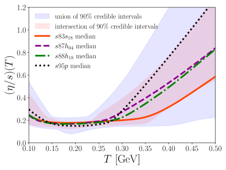
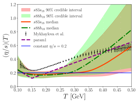
Figure 5: Temperature dependence of $\eta/s$. Upper figure: Median of $\eta/s$ w.r.t. $T$ for each EoS with the union and intersection of the 90% credible intervals of the distributions. Lower figure: Median of $\eta/s$ w.r.t. $T$ for the $s83s_{18}$ and $s88h_{18}$ parametrizations with corresponding credibility intervals compared with two results from Ref. Niemi:2015qia ($\eta/s=0.2$ and param1) and a recent quasiparticle model prediction by Mykhaylova et al. Mykhaylova:2019wci .

In the upper panel of Fig. 5 we show the median of $(\eta/s)(T)$ for each EoS parametrization, and the union and intersection of the 90% credible intervals of all four distributions. The union of the credibility intervals provides insight on the total uncertainty in the analysis including the uncertainty from the EoS parametrization, whereas the difference between the union and intersection illustrates how much of the uncertainty comes from the EoS parametrizations. To emphasize the result using state-of-the-art EoSs, the lower panel of Fig. 5 depicts the median and credibility intervals for the parametrizations $s83s_{18}$ and $s88h_{18}$ only. In the same panel two older results from Ref. Niemi:2015qia , and a recent theoretical prediction from Ref. Mykhaylova:2019wci are shown as well. To make it possible to distinguish the credibility intervals for each EoS separately, $\eta/s$ for each EoS at various temperatures with associated uncertainties is shown in Fig. 6.

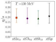
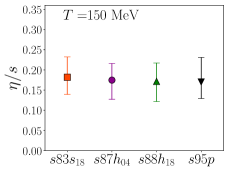
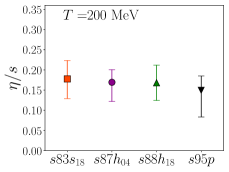
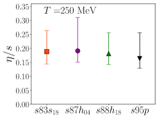
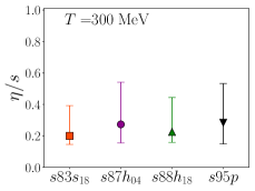
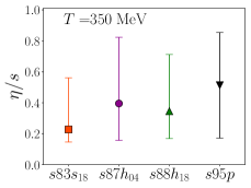
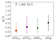
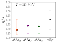
Figure 6: Median values (filled markers) and 90% credible intervals (error bars) for $\eta/s$ at temperatures $T=130,150,200,250,300,350,400$, and $450$ MeV.

We obtain well constrained $\eta/s$ in a temperature range $150\mathrel{\lower 3.87495pt\hbox{$\stackrel{{\scriptstyle\displaystyle<}}{{\sim}}$}}T/\mathrm{MeV}\mathrel{\lower 3.87495pt\hbox{$\stackrel{{\scriptstyle\displaystyle<}}{{\sim}}$}}220$, where the median values of $\eta/s$ are practically constant for all contemporary EoSs, and $s95p$ leads to modest temperature dependence well within the credibility intervals. Within this temperature range $\eta/s$ is constrained between 0.08 and 0.23 by the 90% credible intervals. In particular, for the state-of-the-art EoSs ($s83s_{18}$ and $s88h_{18}$), we obtain even tighter limits $0.12<\eta/s<0.23$ within this range, and the well constrained region extends to slightly higher temperature. For further details see Fig. 5 and Table 2. Interestingly $\eta/s$ at 130 MeV (or at 150 MeV in case of $s95p$) temperature differs from the favored value (median) of the $(\eta/s)_{\mathrm{min}}$ parameter (compare Tables 1 and 2), even if the favored value of the $T_{\mathrm{H}}$ parameter is 130 MeV (or 150 MeV) (see Fig. 4 and Table 1). This seemingly counterintuitive behavior is due to the fat tails of $T_{\mathrm{H}}$ distributions extending to larger temperatures, and thus broadening the region where $S_{\mathrm{HG}}$ affects the $\eta/s$ values. Consequently we see the lowest $\eta/s$ values at $T\approx 200$ MeV temperature (Fig. 5 and Table 2), where the effect of the lower $(\eta/s)_{\mathrm{min}}$ value of the $s95p$ parametrization is also visible.

Table 2: Median values of $\eta/s$ at various temperatures with associated uncertainties (90% credible intervals) from the posterior distributions. Values rounded to two significant figures.

$T$ [MeV]	$s83s_{18}$		$s87h_{04}$		$s88h_{18}$		$s95p$
$130$	$0.19$	${}^{+0.09}_{-0.04}$	$0.19$	${}^{+0.10}_{-0.05}$	$0.19$	${}^{+0.07}_{-0.06}$	$0.21$	${}^{+0.13}_{-0.07}$
$150$	$0.18$	${}^{+0.05}_{-0.04}$	$0.17$	${}^{+0.05}_{-0.04}$	$0.17$	${}^{+0.05}_{-0.05}$	$0.17$	${}^{+0.06}_{-0.04}$
$200$	$0.18$	${}^{+0.04}_{-0.05}$	$0.17$	${}^{+0.03}_{-0.05}$	$0.17$	${}^{+0.04}_{-0.05}$	$0.15$	${}^{+0.04}_{-0.07}$
$250$	$0.19$	${}^{+0.07}_{-0.05}$	$0.19$	${}^{+0.12}_{-0.04}$	$0.18$	${}^{+0.08}_{-0.04}$	$0.16$	${}^{+0.10}_{-0.03}$
$300$	$0.20$	${}^{+0.19}_{-0.05}$	$0.27$	${}^{+0.27}_{-0.11}$	$0.23$	${}^{+0.21}_{-0.07}$	$0.28$	${}^{+0.25}_{-0.13}$
$350$	$0.23$	${}^{+0.33}_{-0.08}$	$0.40$	${}^{+0.42}_{-0.24}$	$0.35$	${}^{+0.36}_{-0.18}$	$0.51$	${}^{+0.34}_{-0.34}$

It is not surprising that we get the best constraints on $\eta/s$ in the temperature range $150\mathrel{\lower 3.87495pt\hbox{$\stackrel{{\scriptstyle\displaystyle<}}{{\sim}}$}}T/\mathrm{MeV}\mathrel{\lower 3.87495pt\hbox{$\stackrel{{\scriptstyle\displaystyle<}}{{\sim}}$}}220$. As was shown in Ref. Niemi:2012ry , the temperature range where $v_{2}$ is most sensitive to the shear viscosity is only slightly broader than this, and higher order anisotropies are sensitive to shear at even narrower temperature ranges.

Even if the uncertainties remain large, we can see qualitative differences in the high temperature behavior of $\eta/s$, where $s95p$ seems to favor earlier and more rapid rise of $\eta/s$ with increasing temperature (Figs. 5 and 6), a difference which is visible in the $S_{\mathrm{QGP}}$ parameter as well (Fig. 4).

Considering earlier results in the literature this is intriguing. Alba et al. Alba:2017hhe used an EoS based on contemporary stout action data called PDG16+/WB2+1, and observed that the reproduction of the LHC data ($\sqrt{s_{\mathrm{NN}}}=5.02$ TeV) required larger constant $\eta/s$ for this EoS than for $s95p$. On the other hand, they were able to use the same value of constant $\eta/s$ for both EoSs to reproduce the RHIC data. They interpreted this to mean that at large temperatures $s95p$ would necessitate lower values of $\eta/s$, but we see an opposite behavior. In a similar fashion we see a difference between the high temperature behavior obtained using the HISQ ($s88h_{18}$ and $s87h_{04}$) and stout action based EoSs ($s83s_{18}$), but the differences are way smaller than the credibility intervals, and thus cannot be considered meaningful.

At temperatures below 150 MeV we again see expanding credibility intervals, and a tendency of $\eta/s$ to increase with decreasing temperature, but hardly any sensitivity to the EoS. Anisotropies measured at RHIC energy are sensitive to the shear viscosity in the hadronic phase Niemi:2012ry ; Niemi:2011ix , and since Schenke et al. in Ref. Schenke:2019ruo saw sensitivity to the EoS using RHIC data only, we would have expected some sensitivity to the EoS at low temperatures. The difference may arise from the bulk viscosity which depended on the EoS as well in Ref. Schenke:2019ruo , or from a different EoS in the hadronic phase. As mentioned, our EoSs are based on known resonance states, whereas the EoSs in Refs. Alba:2017hhe ; Schenke:2019ruo follow the lattice results closely. Better fit to lattice results can be obtained by including predicted but unobserved resonance states in the HRG. We plan to study how the inclusion of these states might affect the results, once we have concocted a plausible scheme for their decays, so that we can evaluate their contribution to the EoS after chemical freeze-out in a consistent manner.

Furthermore, unlike in Ref. Schenke:2019ruo where a hadron cascade was used to describe the evolution in the hadronic phase, in our approach the change in the EoS can also be partly compensated by a change in the freeze-out temperature instead of shear viscosity. As shown in Appendix D, there is indeed an anti-correlation between $T_{\mathrm{dec}}$ and $(\eta/s)_{\mathrm{min}}$. Therefore forcing the system to freeze out at the same temperature, independent of the EoS, would increase the difference in $(\eta/s)_{\mathrm{min}}$. However, the anti-correlation is rather weak $\approx-0.4(-0.2)$ for $s88h_{18}$ ($s95p$), and thus requiring EoS independent $T_{\mathrm{dec}}$ would not change $(\eta/s)_{\mathrm{min}}$ a lot.

Our result of a very slowly rising $\eta/s$ with decreasing temperature in the hadronic phase (i.e., below $T\approx 150$ MeV) may look inconsistent with microscopic calculations predicting relatively large $\eta/s\sim 1$ in the hadronic phase Rose:2017bjz ; Prakash:1993bt ; Csernai:2006zz . However, our result is for a chemically frozen HRG, while the microscopic calculations usually give $\eta/s$ in chemical equilibrium. In the transport model study of Ref. Demir:2008tr , it was shown that nonunit pion and kaon fugacities, i.e. chemical non-equilibrium, can significantly reduce $\eta/s$ in hadron gas. Since, as a first order approximation, $\eta$ depends only weakly on the chemical non-equilibrium Wiranata:2014jda , the main effect is due to $s$: At a given temperature the entropy density $s_{\mathrm{PCE}}$ in a chemically frozen HRG can be significantly larger than the entropy density in chemical equilibrium $s_{\mathrm{CE}}$, and as a consequence $(\eta/s)_{\mathrm{PCE}}$ can be way smaller than $(\eta/s)_{\mathrm{CE}}$. We may thus obtain an approximation for the $\eta/s$ in a chemically equilibrated system as $(\eta/s)_{\mathrm{CE}}=(\eta/s)_{\mathrm{PCE}}(s_{\mathrm{PCE}}/s_{\mathrm{CE}})$ Niemi:2015qia . In our case, where $T_{\mathrm{chem}}=154$ MeV, the ratio of entropies in a chemically frozen to a chemically equilibrated system is $\approx 3.5$ at $T=100$ MeV ($\approx 1.8$ at $T=130$ MeV) which is sufficient to bring our results to the level described in Ref. Csernai:2006zz .

In Fig. 5 we also made a comparison to the earlier results of Ref. Niemi:2015qia and the recent quasiparticle model prediction from Ref. Mykhaylova:2019wci . As expected, the earlier results from Ref. Niemi:2015qia ; Niemi:2015voa are not far from the present analysis, and param1 is practically within the 90% credible interval in the whole temperature range. On the other hand, constant $\eta/s=0.2$ is below the $s95p$ limits at high temperatures, but as discussed, the overall sensitivity to $\eta/s$ at high temperatures is low. Interestingly the prediction of the quasiparticle model of Ref. Mykhaylova:2019wci comes very close to our values for $\eta/s$ around $T_{c}$, although the region where $\eta/s$ is low is narrower than what we found here. This is intriguing, since the quasiparticle model was tuned to reproduce the stout action EoS, i.e., our EoS $s83s_{18}$, which in our analysis leads to the broadest region where $\eta/s$ is almost constant.

The small value of $\eta/s$ and its weak temperature dependence in the temperature range $150\mathrel{\lower 3.87495pt\hbox{$\stackrel{{\scriptstyle\displaystyle<}}{{\sim}}$}}T/\mathrm{MeV}\mathrel{\lower 3.87495pt\hbox{$\stackrel{{\scriptstyle\displaystyle<}}{{\sim}}$}}220$ may indicate that the QGP is strongly coupled not only in the immediate vicinity of $T_{c}$, but in a broader temperature region. This was first proposed in Ref. Shuryak:2003ty , and agrees with the lattice QCD calculations that indicate the presence of hadronlike resonances in QGP in a similar or slightly broader temperature interval Wetzorke:2001dk ; Karsch:2002wv ; Asakawa:2002xj ; Mukherjee:2015mxc . The strongly coupled nature of QGP can also be seen in the large value of the coupling constant defined in terms of the free energy of static quark anti-quark pairs Bazavov:2018wmo . In any case, our result for $(\eta/s)(T)$ is compatible with the lattice QCD calculations, which indicate that weakly coupled QGP picture may be applicable only for $T>350$ MeV Bazavov:2013uja ; Bellwied:2015lba ; Ding:2015fca ; Bazavov:2018wmo .

VI.3 The effect of the parametric form

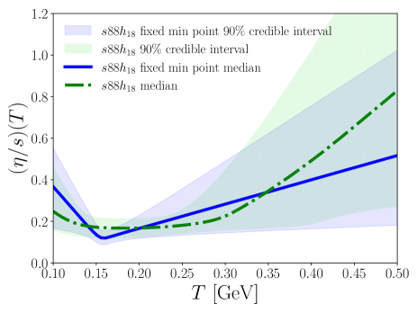
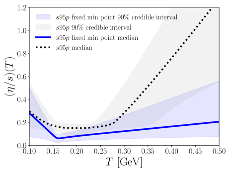
Figure 7: Temperature dependence of $\eta/s$ for the $s88h_{18}$ (top) and $s95p$ (bottom) EoSs using the full parametrization and a parametrization constrained to have a minimum at a fixed point in temperature (“fixed min point”).

When we use the state-of-the-art EoSs ($s88h_{18}$ and $s83s_{18}$), our result for the minimum value of $\eta/s$ is higher than the result obtained in an earlier Bayesian analysis of Ref. Bernhard:2016tnd : $0.12<\eta/s<0.23$ vs. $\eta/s=0.07^{+0.05}_{-0.04}$. While the equations of state in both analyses are based on the latest lattice results, an important difference is that Ref. Bernhard:2016tnd assumed the minimum of $\eta/s$ to occur at fixed $T=154$ MeV temperature, and $\eta/s$ to rise linearly above that temperature. Moreover, below $T=154$ MeV they used a hadron cascade to model the evolution, and the transport properties of the hadronic phase were thus fixed.

To explore how much the results depend on the form of the $(\eta/s)(T)$ parametrization, we mimic the parametrization used in Ref. Bernhard:2016tnd by constraining the plateau in our parametrization to be very small ($0<W_{\mathrm{min}}/\mathrm{MeV}<2$), and the minimum to appear close to $T_{c}$ ($150<T_{\mathrm{H}}/\mathrm{MeV}<160$). The resulting temperature dependence of $\eta/s$ for the $s88h_{18}$ and $s95p$ parametrizations is shown in Fig. 7, and compared to our full result (the behavior of the $s87h_{04}$ and $s83s_{18}$ parametrizations is similar to $s88h_{18}$).

The change in parametrization reduces the minimum value of $\eta/s$ to $0.12^{+0.03}_{-0.03}$ for $s88h_{18}$, which is closest to the EoS used in Ref. Bernhard:2016tnd . The credibility interval now overlaps with the result from the earlier analysis Bernhard:2016tnd , and the results are thus consistent. The remaining difference may result from the bulk viscosity, event-by-event-fluctuations, differences in the EoS parametrization scheme, or the transport description of the hadronic phase. As mentioned earlier, switching to hadron cascade creates a discontinuity in $(\eta/s)(T)$. Enforcing a similar discontinuity in the $(\eta/s)(T)$ parametrization might bring closer the minimum values of $\eta/s$ obtained using hybrid models and continuous fluid dynamics. For $s95p$ the minimum value drops to $0.06^{+0.04}_{-0.04}$, but since the $s95p$ parametrization is based on the older lattice data, comparing this value against Ref. Bernhard:2016tnd is not straightforward. However, due to the significant overlap of the crediblity intervals, we consider both results consistent with Ref. Bernhard:2016tnd , demonstrating the weak sensitivity of the extracted $\eta/s$ to the EoS used in the calculations.

Another interesting change is seen in the high-temperature behavior. In the full analysis the $s95p$ parametrization leads to the largest $\eta/s$ at large temperatures, but the restricted parametrization causes $s95p$ to favor the lowest $\eta/s$ at large temperatures. As seen previously, $s95p$ favors the lowest $\eta/s$ at $200<T/\mathrm{MeV}<250$ temperatures (see Fig. 6 and Table 2), which in the restricted parametrization dictates the behavior at much higher temperatures as well.

Nevertheless, even if the results depend on the form of the parametrization, the credibility intervals overlap and the results are consistent. The only deviation from this rule is for the $s95p$ parametrization around $T=160$ MeV temperature where the difference is statistically significant (see Fig. 7). We have also checked that when we use the favored parameter values, the typical differences in the fit to the data due to different parametric forms are only $\approx(1-3)\%$.

Similarly, we can mimic temperature independent $\eta/s$ by constraining the priors of the $S_{\mathrm{HG}}$ and $S_{\mathrm{QGP}}$ parameters close to zero. We have checked that such a choice does not increase the sensitivity of $\eta/s$ to the EoS parametrization, and that the median values of the constant $\eta/s=(\eta/s)_{\mathrm{min}}$ were only $\approx 10\%$ larger than the median values for $\eta/s$ at $T=200$ MeV for the full parametrization. Again, a sign of $v_{2}$ being most sensitive to shear viscosity in the $150\mathrel{\lower 3.87495pt\hbox{$\stackrel{{\scriptstyle\displaystyle<}}{{\sim}}$}}T/\mathrm{MeV}\mathrel{\lower 3.87495pt\hbox{$\stackrel{{\scriptstyle\displaystyle<}}{{\sim}}$}}220$ temperature range Niemi:2012ry .

Thus, in the Bayesian analysis the parametric form of $\eta/s$ does affect the results, and is therefore a kind of prior whose effects are difficult to quantify. On the other hand, the credibility intervals overlap in all the cases, which emphasizes their importance: The “true” value could be anywhere within the credibility interval, and there is still a 10% chance it is outside of it.

VI.4 Comparison with the data

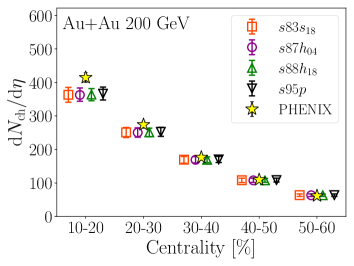
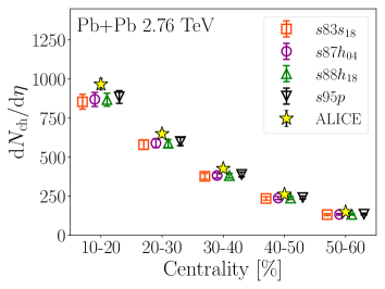
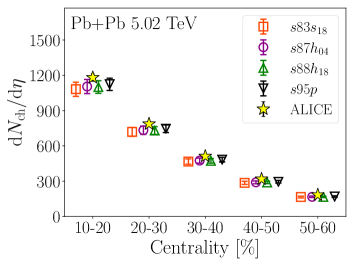
Figure 8: Charged particle multiplicity at various centralities using 1000 samples from the posterior distribution of each EoS. Marker centers indicate median values, and error bars 90% credible intervals. Top panel: Au+Au at $\sqrt{s_{\mathrm{NN}}}=200$ GeV compared to PHENIX data Adler:2004zn . Middle panel: Pb+Pb at $\sqrt{s_{\mathrm{NN}}}=2.76$ TeV compared to ALICE data Aamodt:2010cz . Bottom panel: Pb+Pb at $\sqrt{s_{\mathrm{NN}}}=5.02$ TeV compared to ALICE data Adam:2015ptt .

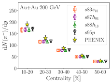
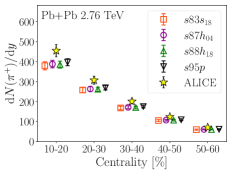
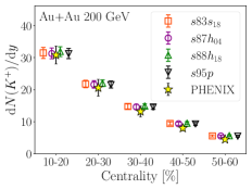
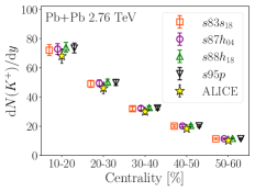
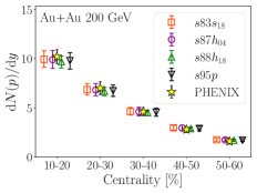
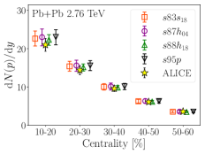
Figure 9: Pion (upper panels), kaon (middle panels), and proton (lower panels) multiplicities at various centralities using 1000 samples from the posterior distribution of each EoS. Marker centers indicate median values, and error bars 90% credible intervals. Left panels: Au+Au at $\sqrt{s_{\mathrm{NN}}}=200$ GeV compared to PHENIX data Adler:2003cb . Right panels: Pb+Pb at $\sqrt{s_{\mathrm{NN}}}=2.76$ TeV compared to ALICE data Abelev:2013vea

.

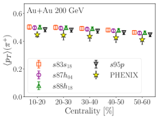
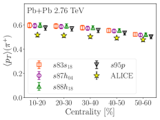
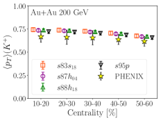
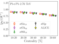
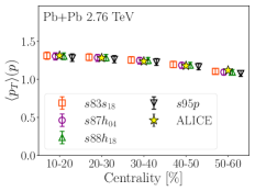
Figure 10: As Fig. 9 but for the mean transverse momentum.

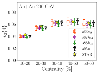
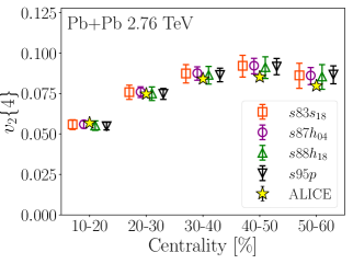
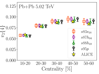
Figure 11: Charged particle elliptic flow $v_{2}\{4\}$ at various centralities using 1000 samples from the posterior distribution of each EoS. Marker centers indicate median values, and error bars 90% credible intervals. Left panel: Au+Au at $\sqrt{s_{\mathrm{NN}}}=200$ GeV compared to STAR data Adams:2004bi . Middle panel: Pb+Pb at $\sqrt{s_{\mathrm{NN}}}=2.76$ TeV compared to ALICE data Adam:2016izf . Right panel: Pb+Pb at $\sqrt{s_{\mathrm{NN}}}=5.02$ TeV compared to ALICE data Adam:2016izf .

Finally, as an overall quality check, we show how well the favored parameter combinations reproduce the experimental data. This is done by drawing 1000 samples from each posterior distribution and using the Gaussian process emulator to predict the simulation output for these values. The results for charged and identified particle multiplicities, identified particle $\langle p_{T}\rangle$, and the elliptic flow $v_{2}\{4\}$ are shown in Figs. 8, 9, 10, and 11, respectively.

The overall agreement with the data is quite good for all observables, and the analysis is able to find equally good data fits for all four EoSs. As normal for thermal models, the charged particle multiplicities tend to be underestimated due to the tension between pion multiplicity on one hand, and kaon and proton multiplicities on the other hand. As the analysis makes a compromise between too few pions and too many kaons and protons, the overall charged particle multiplicity (which is dominated by pions) will remain below the data. Also the mean transverse momentum of pions is slightly too large, which may prove difficult to alleviate without the introduction of bulk viscosity Ryu:2015vwa and/or improved treatment of resonances during the hadronic phase Huovinen:2016xxq .

VII Summary

In this work, we have introduced three new parametrizations of the equation of state based on the contemporary lattice data:

• $s87h_{04}$ connects the HRG based on the PDG 2004 particle list to parametrized lattice data obtained using the HISQ discretization scheme.

• $s88h_{18}$ is based on the HRG containing all strange and non-strange hadrons and resonances in the PDG 2018 summary tables, and the same HISQ lattice data as $s87h_{04}$.

• $s83s_{18}$ is constructed using the PDG 2018 resonances, and the continuum extrapolated lattice data obtained using the stout discretization.

We used these new parametrizations and the older $s95p$ parametrization to examine how sensitive the shear viscosity over entropy density ratio $\eta/s$ is to the equation of state. We assumed a piecewise linear parametrization for $(\eta/s)(T)$, and determined the probability distributions of the best-fit parameter values within the EKRT framework using a Bayesian statistics approach.

Using charged and identified particle multiplicities, identified particle mean transverse momenta, and elliptic flow at three different collision energies as calibration data, we were able to constrain the value of $\eta/s$ to be between 0.08 and 0.23 with 90% credibility in the temperature range $150\mathrel{\lower 3.87495pt\hbox{$\stackrel{{\scriptstyle\displaystyle<}}{{\sim}}$}}T/\mathrm{MeV}\mathrel{\lower 3.87495pt\hbox{$\stackrel{{\scriptstyle\displaystyle<}}{{\sim}}$}}220$ when all EoS parametrizations are taken into account. When we constrain the EoSs to the most contemporary parametrizations $s83s_{18}$ and $s88h_{18}$, we obtain $0.12<\eta/s<0.23$ in the above mentioned temperature range. As the differences between the EoSs are well covered by the 90% credible intervals, the earlier results obtained using the $s95p$ parametrization remain valid. The weak sensitivity to the EoS is consistent with the old ideal fluid results for flow and EoS: Based on flow alone, it is difficult to distinguish an EoS with a smooth crossover from an EoS without phase transition Huovinen:2005gy . Thus when the differences between EoSs are just details in the crossover, the differences in flow, which should be compensated by different shear viscosity, are small, and consequently differences in the extracted $\eta/s$ are small.

The overall agreement with the data is quite good, and similar to Refs. Niemi:2015qia ; Niemi:2015voa , where event-by-event fluctuations were included to the framework of EKRT initial conditions and fluid dynamics, albeit without the Bayesian analysis. The good agreement achieved here is partly due to the EKRT initial conditions. In particular the centrality and $\sqrt{s_{\mathrm{NN}}}$ dependence of hadron multiplicities follow mainly from the QCD dynamics of the EKRT model. A noticeable difference to the earlier event-by-event analysis is that here we used identified hadron multiplicities as constraint, which led to the chemical freeze-out temperature $T_{\mathrm{chem}}\approx 154$ MeV, and a slight overshoot of the pion average $p_{T}$ compared to the data. In the earlier analysis $T_{\mathrm{chem}}\approx 175$ MeV was used to reproduce the average $p_{T}$ data, which in turn led to too large proton multiplicity. It is possible to solve this tension by introducing bulk viscosity Ryu:2015vwa , but that is left for a future work. We emphasize that compared to the (in principle) more detailed hydro + cascade models our hydro + partial chemical equilibrium approach has two major advantages: It allows us to parametrize $(\eta/s)(T)$ so that it is continuous in the whole temperature range, and at the same time it gives us a possibility to constrain the viscosity also in the hadronic phase.

Inclusion of event-by-event fluctuations to the analysis would provide access to several new flow observables such as higher flow harmonics $v_{n}$, and flow correlations, which may give tighter constraints in broader temperature interval on $(\eta/s)(T)$. However, within the current uncertainties of the fitting procedure, we cannot exclude the possibility that the effect of the EoS remains negligible even when $\eta/s$ at $T>220$ MeV becomes better under control.

Since the sensitivity of flow to shear viscosity at high temperatures is low, observables based on high $p_{T}$ particles may be useful to constrain, not only the pre-equilibrium dynamics Noronha-Hostler:2016eow ; Andres:2019eus ; Zigic:2019sth , but also the properties of the fluid when it is hottest.

Appendix A EoS parametrization

Table 3: The values of parameters for different fits of the trace anomaly.

	$d_{0}$	$d_{1}$(GeV2)	$d_{2}$(GeV4)	$d_{3}$(GeV${}^{n_{3}}$)	$d_{4}$(GeV${}^{n_{4}}$)	$d_{5}$(GeV${}^{n_{5}}$)	$n_{3}$	$n_{4}$	$n_{5}$	$T_{0}$(MeV)
$s83s_{18}$	5.688$\times 10^{-3}$	$0.3104$	-6.217$\times 10^{-3}$	-6.680$\times 10^{-32}$	1.071$\times 10^{-32}$	–	41	42	–	$166$
$s87h_{04}$	5.669$\times 10^{-2}$	$0.2974$	-4.184$\times 10^{-3}$	-5.146$\times 10^{-8}\,\,$	1.420$\times 10^{-33}$	–	10	42	–	$172$
$s88h_{18}$	4.509$\times 10^{-2}$	$0.3082$	-5.136$\times 10^{-3}$	-1.150$\times 10^{-10}$	2.076$\times 10^{-32}$	-3.021$\times 10^{-33}$	13	41	42	$155$
$s95p$	–	$0.2660$	2.403$\times 10^{-3}$	-2.809$\times 10^{-7}\,\,$	6.073$\times 10^{-23}$	–	10	30	–	$183.8$

Table 4: The values of parameters for different fits of the HRG trace anomaly.

	$a_{1}$(GeV${}^{-m_{1}}$)	$a_{2}$(GeV${}^{-m_{2}}$)	$a_{3}$(GeV${}^{-m_{3}}$)	$a_{4}$(GeV${}^{-m_{4}}$)	$m_{1}$	$m_{2}$	$m_{3}$	$m_{4}$	$T_{\mathrm{high}}$(MeV)
$s83s_{18}$	$0.1850$	1.985$\times 10^{4}$	1.278$\times 10^{5}$	-1.669$\times 10^{7}$	0	5	7	10	170
$s87h_{04}$	$4.654\;\;$	-$879\quad\;\,$	$8081\quad\;\,$	-7.039$\times 10^{6}$	1	3	4	10	190
$s88h_{18}$	$0.1844$	2.043$\times 10^{4}$	8.550$\times 10^{5}$	-2.434$\times 10^{7}$	0	5	8	10	169
$s95p$	$4.654\;\;$	-$879\quad\;\,$	$8081\quad\;\,$	-7.039$\times 10^{6}$	1	3	4	10	190

At high temperature the trace anomaly can be well parametrized by the inverse polynomial form. Therefore we will use the following Ansatz for the high temperature region:

$$\frac{\epsilon-3p}{T^{4}}=d_{0}+\frac{d_{1}}{T^{2}}+\frac{d_{2}}{T^{4}}+\frac{d_{3}}{T^{n_{3}}}+\frac{d_{4}}{T^{n_{4}}}+\frac{d_{5}}{T^{n_{5}}}.$$ (8)

This form does not have the right asymptotic behavior in the high temperature region, where we expect $(\epsilon-3p)/T^{4}\sim g^{4}(T)\sim 1/\ln^{2}(T/\Lambda_{QCD})$, but it works well in the temperature range of interest. Furthermore, it is flexible enough to match to the HRG result in the low temperature region. We match this Ansatz to the HRG model at temperature $T_{0}$ by requiring that the trace anomaly, and its first and second derivatives are continuous. This requirement provides constraints for three parameters, $d_{0},d_{1},$ and $d_{2}$, and leaves the remaining seven, $d_{3},d_{4},d_{5},n_{3},n_{4},n_{5},$ and $T_{0}$ to be fixed by minimizing a $\chi^{2}$ fit to the data. Fitting the powers $n_{3}$–$n_{5}$ would be a highly non-linear problem, but we simplify the problem by requiring that the powers are integers, and using brute force: We make a fit with all the integer values $5\leq n_{3}\leq 40$, $n_{3}<n_{4}\leq 41$, and $n_{4}<n_{5}\leq 42$, and choose the values $n_{3},n_{4}$, and $n_{5}$ which lead to the smallest $\chi^{2}$. When the powers and $T_{0}$ are kept fixed, minimizing $\chi^{2}$ requires only a simple matrix inversion. Thus to fix $T_{0}$ we are able to cast $\chi^{2}$ as a function of only a single parameter, $T_{0}$. We require that $155\leq T_{0}/\mathrm{MeV}\leq 190$, and search for the value of $T_{0}$ which minimizes $\chi^{2}$.

To obtain the continuum limit in the lattice calculations of the trace anomaly, one has to perform interpolation in the temperature, and then perform continuum extrapolations (see e.g. Borsanyi:2013bia ). This procedure can introduce additional uncertainties when providing parametrization of the lattice results. As mentioned in the main text, the lattice spacing ($N_{t}$) dependence of the lattice results is small in the case of the HISQ discretization scheme for $N_{t}\geq 8$. In fact, for $T>230$ MeV and $T<170$ MeV there is no statistically significant $N_{t}$ dependence, so in these temperature ranges we can use the HISQ lattice results with $N_{t}=8,10$ and $12$. In the peak region, $170<T/\mathrm{MeV}<230$, the $N_{t}=8$ HISQ results are slightly higher than the $N_{t}=10$ and $N_{t}=12$ results, and therefore have been omitted from the fits. At temperatures above $800$ MeV only lattice results with $N_{t}=6$ and 4 are available Bazavov:2014pvz ; Bazavov:2017dsy . To take the larger discretization errors of the $N_{t}=6$ and 4 results into account, we follow Ref. Bazavov:2017dsy , scale them by factors 1.4 and 1.2, and include systematic errors of 40% and 20%, respectively. Contrary to the HISQ action results, we employ the continuum extrapolated stout action results Borsanyi:2013bia ; Borsanyi:2010cj for simplicity. The resulting parameters are shown in Table 3. We find that only the parametrization $s88h_{18}$ requires the use of all six terms in Eq. 8. In the cases of $s83s_{18}$ and $s87h_{04}$ we are able to obtain equally good fits with only five terms, and thus set $d_{5}$ to zero by hand.

For the sake of completeness, we also parametrize the HRG part of the trace anomaly as

$$\frac{\epsilon-3p}{T^{4}}=a_{1}T^{m_{1}}+a_{2}T^{m_{2}}+a_{3}T^{m_{3}}+a_{4}T^{m_{4}}.$$ (9)

To carry out the fit we evaluate HRG trace anomaly in temperature interval $70<T/\mathrm{MeV}<T_{\mathrm{high}}$, where $T_{\mathrm{high}}$ depends on the parametrization, with 1 MeV steps assuming that each point has equal “error”. The limits have entirely utilitarian origin: in hydrodynamical applications the system decouples well above 70 MeV temperature and only a rough approximation of the EoS, $p=p(\epsilon)$, is needed at lower temperatures. On the other hand we expect to switch to the lattice parametrization below $T_{\mathrm{high}}$, and the HRG EoS above that temperature is not needed either. We fix the powers in Eq. (9) again using brute force. We require them to be integers, go through all the combinations $0\leq l_{1}<l_{2}<l_{3}<l_{4}\leq 10$, fit the parameters $a_{1}$, $a_{2}$, $a_{3}$, $a_{4}$ to the HRG trace anomaly evaluated with 1 MeV intervals, and choose the values $l_{1},~{}l_{2},~{}l_{3}$ and $l_{4}$ which minimize the $\chi^{2}$. We end up with parameters shown in Table 4. To obtain the EoS, one also needs the pressure at the lower limit of the integration (see Eq.(1)) $T_{\mathrm{low}}=0.07$ GeV: $p(T_{\mathrm{low}})/T^{4}_{\mathrm{low}}=0.1661$. Our EoSs are available in a tabulated form at arXiv as ancillary files for this paper, and at Ref. osf . These tables also include the option of a chemically frozen hadronic stage, and a list of resonances included in the hadronic stage with their properties and decay channels.

Appendix B Predicting model output with Gaussian processes

Let us assume that we do not know exactly what the model’s output $y$ for a particular input parameter $\vec{x}$ is, but we know its most probable value $\mu(\vec{x})$. We postulate that the probability distribution for the output value $P(y)$ is a normal distribution with mean $\mu(\vec{x})$ and so far unknown width $\sigma$. Thus the probability distribution for a set $Y_{a}$ of $N$ model outputs for observable $a$, corresponding to a set $X$ of $N$ points in the parameter space, is a multivariate normal distribution:

$$\mathcal{G}:X\rightarrow Y_{a}\sim\mathcal{N}(\boldsymbol{\mu},\boldsymbol{C})$$ (10)

where $\boldsymbol{\mu}=\mu(X)=\{\mu(\vec{x}_{1}),\ldots,\mu(\vec{x}_{N})\}$ is the mean of the distribution, and $\boldsymbol{C}$ is the covariance matrix defined by the covariance function $c(\vec{x},\vec{x}^{\prime})$:

$$\boldsymbol{C}=\mathcal{C}_{X,X}=\begin{pmatrix}c(\vec{x}_{1},\vec{x}_{1})&\dots&c(\vec{x}_{1},\vec{x}_{N})\\ \vdots&\ddots&\vdots\\ c(\vec{x}_{N},\vec{x}_{1})&\dots&c(\vec{x}_{N},\vec{x}_{N})\\ \end{pmatrix}.$$ (11)

As we are only interested in interpolating within the training data, we may set $\mu(X)\equiv 0$, and construct the covariance function $c(\vec{x},\vec{x}^{\prime})$ in such a way that the probability distribution is narrow at the training points nevertheless. This way we minimize our a priori assumptions about the model behavior in regions of parameter space not covered by the training data. Our chosen covariance function is a radial-basis function (RBF) with a noise term

$$c(\vec{x},\vec{x}^{\prime})=\theta_{0}\exp\left(-\sum\limits_{i=1}^{n}\frac{(x_{i}-x^{\prime}_{i})^{2}}{2\theta_{i}^{2}}\right)+\theta_{\text{noise}}\delta_{\vec{x}\vec{x}^{\prime}}$$ (12)

The hyperparameters $\vec{\theta}=(\theta_{0},\theta_{1},\ldots,\theta_{n},\theta_{\text{noise}})$, where $n$ is the dimension of the input parameter space, are not known a priori and must be estimated from training data, consisting of simulation output $U$ computed at training points $T$, by maximizing the log-likelihood (see Chapter 5 of Rasmussen:2006 )

$$\begin{split}\log P(U|T,\vec{\theta})=&-\frac{1}{2}U^{T}\boldsymbol{C}^{-1}(T,\vec{\theta})U\\ &-\frac{1}{2}\log|\boldsymbol{C}(T,\vec{\theta})|\\ &-\frac{N}{2}\log(2\pi).\end{split}$$ (13)

Emulator prediction for the model output $y_{0}$ at a point $\vec{x_{0}}$ can then be determined by writing a joint probability distribution for the output at various points in parameter space:

$$\begin{pmatrix}y_{0}\\ U\end{pmatrix}\sim\mathcal{N}\left(\begin{pmatrix}0\\ \vec{0}\end{pmatrix},\begin{pmatrix}\mathcal{C}_{0,0}&\mathcal{C}_{0,T}\\ \mathcal{C}_{T,0}&\mathcal{C}_{T,T}\end{pmatrix}\right)$$ (14)

from which we can derive the conditional predictive mean $y^{\text{GP}}(\vec{x_{0}})$ and associated variance $\sigma^{\text{GP}}(\vec{x_{0}})^{2}$ as (see e.g. Appendix A.2 of Rasmussen:2006 )

$$\begin{split}y^{\text{GP}}(\vec{x_{0}})&=\mathcal{C}_{0,T}\mathcal{C}_{T,T}^{-1}U,\\ \sigma^{\text{GP}}(\vec{x_{0}})^{2}&=\mathcal{C}_{0,0}-\mathcal{C}_{0,T}\mathcal{C}_{T,T}^{-1}\mathcal{C}_{T,0}.\end{split}$$ (15)

Note that we use the training data $U$ twice: First in Eq. (13) to determine the hyperparameters $\vec{\theta}$ of the covariance function $c(\vec{x},\vec{x}^{\prime})$ and then in Eq. (15) as a condition for the GP prediction.

Appendix C Principal component analysis

We reduce the number of Gaussian processes needed for model emulation with principal component analysis (PCA), which transforms the data in the directions of maximal variance.

We represent the model output with a $N$ x $m$ matrix $Y$, where $N$ is the number of simulation points and $m$ the number of observables. In preparation for the PCA, the data columns are normalized with the corresponding experimental values to obtain dimensionless quantities, and centered by subtracting the mean of each observable from the elements of each column; we denote this scaled and shifted data matrix by $\hat{Y}$.

We then want to find an eigenvalue decomposition of the covariance matrix $\hat{Y}^{T}\hat{Y}$:

$$\hat{Y}^{T}\hat{Y}=V\Lambda V^{T},$$ (16)

where $\Lambda$ is the diagonal matrix containing the eigenvalues $\lambda_{1},...,\lambda_{m}$ and $V$ is an orthogonal matrix containing the eigenvectors of the covariance matrix.

The eigenvalue decomposition is found by factorizing $\hat{Y}$ via the singular value decomposition:

$$\hat{Y}=USV^{T},$$ (17)

where $S$ is a diagonal matrix containing the singular values (square roots of the eigenvalues of $\hat{Y}^{T}\hat{Y}$) and $V$ contains the right-singular vectors of $\hat{Y}$ (eigenvectors of $\hat{Y}^{T}\hat{Y}$); these are the principal components (PCs). Matrix $U$ contains the left-singular vectors of $\hat{Y}$, which are eigenvectors of $\hat{Y}\hat{Y}^{T}$.

The eigenvalues are proportional to the total variance of the data. Since $\lambda_{1}\geq\lambda_{2}\geq...\geq\lambda_{m}$, the fraction of the total variance explained by the $k$th principal component, $\lambda_{k}/(\sum\limits_{j=1}^{m}\lambda_{j})$, becomes negligible starting from some index $k<m$. This allows us to define a lower-rank approximation of the original transformed data matrix $Z=\hat{Y}V$ as $Z_{k}=\hat{Y}V_{k}$, where $V_{k}$ contains the first $k$ columns of $V$.

The transformation of a vector $\vec{y}$ from the space of observables to a vector $\vec{z}$ in the reduced-dimension principal component space is thus defined as

$$\vec{z}=\vec{y}\,V_{k},$$ (18)

while for matrices (such as the covariance matrix in the likelihood function (V)) the transformation is

$$\Sigma_{z}=V_{k}^{T}\,\Sigma_{y}\,V_{k}.$$ (19)

To compare an emulator prediction $\vec{z}^{\,\text{GP}}$ against physical observables, we use the inverse transformation

$$\vec{y}^{\,\text{GP}}=\vec{z}^{\,\text{GP}}\,V_{k}^{T}.$$ (20)

Appendix D Correlations between the model parameters

Figure 12 provides a more detailed view of the 8-dimensional posterior probability distribution, using the analysis results for the $s88h_{18}$ and $s95p$ EoSs as an example. The diagonal panels show the marginalized one-dimensional distributions for each parameter, which were summarized in Figs. 3–4 in Section VI. The off-diagonal panels illustrate the correlations between each parameter pair $(X,Y)$. The correlation strength is quantified with the Spearman rank correlation coefficient Spearman:1904 , which is the Pearson correlation coefficient between the rank values $r_{X}$ and $r_{Y}$:

$$\rho=\frac{C(r_{X},r_{Y})}{\sigma(r_{X})\sigma(r_{Y})},$$ (21)

where $C$ refers to covariance and $\sigma$ to standard deviation. This relaxes the assumption of a linear relationship, present in the Pearson correlation coefficient, and is instead a measure of the monotonic relationship between the two parameters.

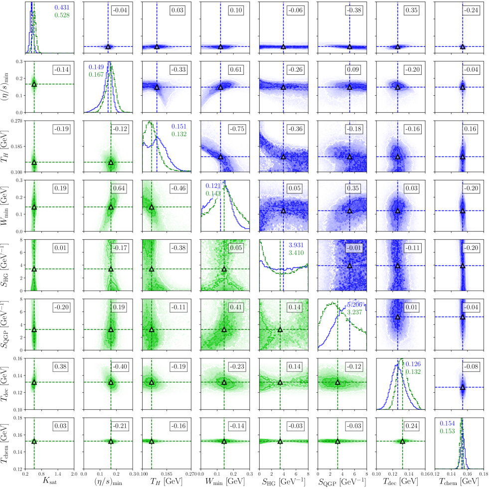
Figure 12: Posterior probability distribution for the $s88h_{18}$ (lower triangle, green color) and $s95p$ (upper triangle, blue color) EoSs. Diagonal panels: Marginalized 1-D distributions for each parameter. Solid blue line: $s95p$. Dash-dotted green line: $s88h_{18}$. Dashed lines and numbers indicate median value, with upper number corresponding to $s95p$ and lower number to $s88h_{18}$. Off-diagonal panels: 2-D projections of the posterior distributions. Dashed lines indicate median values for each parameter, while the framed numbers refer to Spearman rank correlation coefficients for each parameter pair.

References

- (1) M. Luzum and P. Romatschke, Phys. Rev. C 78, 034915 (2008) Erratum: [Phys. Rev. C 79, 039903 (2009)] [arXiv:0804.4015 [nucl-th]].
- (2) P. Bozek, Phys. Rev. C 81, 034909 (2010) [arXiv:0911.2397 [nucl-th]].
- (3) H. Song, S. A. Bass and U. Heinz, Phys. Rev. C 83, 054912 (2011) Erratum: [Phys. Rev. C 87, 019902 (2013)] [arXiv:1103.2380 [nucl-th]].
- (4) S. Ryu, J.-F. Paquet, C. Shen, G. S. Denicol, B. Schenke, S. Jeon and C. Gale, Phys. Rev. Lett. 115, 132301 (2015) [arXiv:1502.01675 [nucl-th]].
- (5) I. A. Karpenko, P. Huovinen, H. Petersen and M. Bleicher, Phys. Rev. C 91, 064901 (2015) [arXiv:1502.01978 [nucl-th]].
- (6) U. Heinz and R. Snellings, Ann. Rev. Nucl. Part. Sci. 63, 123 (2013) [arXiv:1301.2826 [nucl-th]].
- (7) C. Gale, S. Jeon and B. Schenke, Int. J. Mod. Phys. A 28, 1340011 (2013) [arXiv:1301.5893 [nucl-th]].
- (8) P. Huovinen, Int. J. Mod. Phys. E 22, 1330029 (2013) [arXiv:1311.1849 [nucl-th]].
- (9) C. Shen, [arXiv:2001.11858 [nucl-th]].
- (10) J. E. Bernhard, J. S. Moreland, S. A. Bass, J. Liu and U. Heinz, Phys. Rev. C 94, 024907 (2016) [arXiv:1605.03954 [nucl-th]].
- (11) S. A. Bass, J. E. Bernhard and J. S. Moreland, Nucl. Phys. A 967, 67 (2017) [arXiv:1704.07671 [nucl-th]].
- (12) J. E. Bernhard, J. S. Moreland and S. A. Bass, Nature Phys. 15, no. 11, 1113 (2019).
- (13) H. Niemi, K. J. Eskola and R. Paatelainen, Phys. Rev. C 93, 024907 (2016) [arXiv:1505.02677 [hep-ph]].
- (14) S. Pratt, E. Sangaline, P. Sorensen and H. Wang, Phys. Rev. Lett. 114, 202301 (2015) [arXiv:1501.04042 [nucl-th]].
- (15) J. S. Moreland and R. A. Soltz, Phys. Rev. C 93, 044913 (2016) [arXiv:1512.02189 [nucl-th]].
- (16) P. Alba, V. Mantovani Sarti, J. Noronha, J. Noronha-Hostler, P. Parotto, I. Portillo Vazquez and C. Ratti, Phys. Rev. C 98, 034909 (2018) [arXiv:1711.05207 [nucl-th]].
- (17) P. Huovinen and P. Petreczky, Nucl. Phys. A 837, 26 (2010) [arXiv:0912.2541 [hep-ph]].
- (18) A. Bazavov et al., Phys. Rev. D 80, 014504 (2009) [arXiv:0903.4379 [hep-lat]].
- (19) B. Schenke, C. Shen and P. Tribedy, Phys. Rev. C 99, 044908 (2019) [arXiv:1901.04378 [nucl-th]].
- (20) A. Bazavov et al. [HotQCD Collaboration], Phys. Rev. D 90, 094503 (2014) [arXiv:1407.6387 [hep-lat]].
- (21) A. Bazavov, P. Petreczky and J. H. Weber, Phys. Rev. D 97, 014510 (2018) [arXiv:1710.05024 [hep-lat]].
- (22) S. Borsanyi, G. Endrodi, Z. Fodor, A. Jakovac, S. D. Katz, S. Krieg, C. Ratti and K. K. Szabo, JHEP 1011, 077 (2010) [arXiv:1007.2580 [hep-lat]].
- (23) S. Borsanyi, Z. Fodor, C. Hoelbling, S. D. Katz, S. Krieg and K. K. Szabo, Phys. Lett. B 730, 99 (2014) [arXiv:1309.5258 [hep-lat]].
- (24) H. Niemi, K. J. Eskola, R. Paatelainen and K. Tuominen, Phys. Rev. C 93, 014912 (2016) [arXiv:1511.04296 [hep-ph]].
- (25) S. Adler et al. [PHENIX], Phys. Rev. C 71, 034908 (2005). [arXiv:nucl-ex/0409015 [nucl-ex]].
- (26) S. S. Adler et al. [PHENIX Collaboration], Phys. Rev. C 69, 034909 (2004) [nucl-ex/0307022].
- (27) J. Adams et al. [STAR Collaboration], Phys. Rev. C 72, 014904 (2005) [nucl-ex/0409033].
- (28) K. Aamodt et al. [ALICE Collaboration], Phys. Rev. Lett. 106, 032301 (2011) [arXiv:1012.1657 [nucl-ex]].
- (29) B. Abelev et al. [ALICE Collaboration], Phys. Rev. C 88, 044910 (2013) [arXiv:1303.0737 [hep-ex]].
- (30) J. Adam et al. [ALICE Collaboration], Phys. Rev. Lett. 116, 132302 (2016) [arXiv:1602.01119 [nucl-ex]].
- (31) J. Adam et al. [ALICE Collaboration], Phys. Rev. Lett. 116, 222302 (2016) [arXiv:1512.06104 [nucl-ex]].
- (32) G. Boyd, J. Engels, F. Karsch, E. Laermann, C. Legeland, M. Lutgemeier and B. Petersson, Nucl. Phys. B 469, 419 (1996) [arXiv:hep-lat/9602007].
- (33) C. Anderlik et al., Phys. Rev. C 59, 3309 (1999) [arXiv:nucl-th/9806004].
- (34) P. Huovinen and P. Petreczky, PoS Confinement 2018, 145 (2019) [arXiv:1811.09330 [nucl-th]].
- (35) S. A. Bass et al., Prog. Part. Nucl. Phys. 41, 255 (1998) [nucl-th/9803035]; M. Bleicher et al., J. Phys. G 25, 1859 (1999) [hep-ph/9909407].
- (36) J. Weil et al., Phys. Rev. C 94, 054905 (2016) [arXiv:1606.06642 [nucl-th]].
- (37) S. Eidelman et al. [Particle Data Group], Phys. Lett. B 592, 1 (2004).
- (38) R. Venugopalan and M. Prakash, Nucl. Phys. A 546, 718-760 (1992).
- (39) W. Broniowski, F. Giacosa and V. Begun, Phys. Rev. C 92, 034905 (2015) [arXiv:1506.01260 [nucl-th]].
- (40) M. Tanabashi et al. [Particle Data Group], Phys. Rev. D 98, 030001 (2018).
-
(41)
Non-strange meson summary tables:
http://pdg.lbl.gov/2018/tables/rpp2018-tab-mesons-light.pdf;
Strange mesons:
http://pdg.lbl.gov/2018/tables/rpp2018-tab-mesons-strange.pdf;
p, n, and N resonances: http://pdg.lbl.gov/2018/tables/rpp2018-tab-baryons-N.pdf;
Lambda, Lambda resonances: http://pdg.lbl.gov/2018/tables/rpp2018-tab-baryons-Lambda.pdf;
Sigma, Sigma resonances: http://pdg.lbl.gov/2018/tables/rpp2018-tab-baryons-Sigma.pdf;
Xi, Xi resonances: http://pdg.lbl.gov/2018/tables/rpp2018-tab-baryons-Xi.pdf;
Omega, Omega resonances: http://pdg.lbl.gov/2018/tables/rpp2018-tab-baryons-Omega.pdf. - (42) A. Majumder and B. Muller, Phys. Rev. Lett. 105, 252002 (2010) [arXiv:1008.1747 [hep-ph]].
- (43) A. Bazavov et al., Phys. Rev. Lett. 113, 072001 (2014) [arXiv:1404.6511 [hep-lat]].
- (44) C. Fernández-Ramírez, P. M. Lo and P. Petreczky, Phys. Rev. C 98, 044910 (2018) [arXiv:1806.02177 [hep-ph]].
- (45) P. Alba, V. M. Sarti, J. Noronha-Hostler, P. Parotto, I. Portillo-Vazquez, C. Ratti and J. Stafford, Phys. Rev. C 101, 054905 (2020) [arXiv:2002.12395 [hep-ph]].
- (46) H. Niemi, G. S. Denicol, P. Huovinen, E. Molnar and D. H. Rischke, Phys. Rev. C 86, 014909 (2012) [arXiv:1203.2452 [nucl-th]].
- (47) H. Niemi, G. S. Denicol, P. Huovinen, E. Molnar and D. H. Rischke, Phys. Rev. Lett. 106, 212302 (2011) [arXiv:1101.2442 [nucl-th]].
- (48) K. J. Eskola, H. Niemi, R. Paatelainen and K. Tuominen, Phys. Rev. C 97,, 034911 (2018) [arXiv:1711.09803 [hep-ph]].
- (49) E. Molnar, H. Niemi and D. H. Rischke, Eur. Phys. J. C 65, 615 (2010) [arXiv:0907.2583 [nucl-th]].
- (50) W. Israel and J. M. Stewart, Annals Phys. 118, 341 (1979).
- (51) G. S. Denicol, H. Niemi, E. Molnar and D. H. Rischke, Phys. Rev. D 85, 114047 (2012) Erratum: [Phys. Rev. D 91, 039902 (2015)] [arXiv:1202.4551 [nucl-th]].
- (52) E. Molnar, H. Niemi, G. S. Denicol and D. H. Rischke, Phys. Rev. D 89, 074010 (2014) [arXiv:1308.0785 [nucl-th]].
- (53) P. Huovinen, Eur. Phys. J. A 37, 121 (2008) [arXiv:0710.4379 [nucl-th]].
- (54) T. Hirano and K. Tsuda, Phys. Rev. C 66, 054905 (2002) [arXiv:nucl-th/0205043 [nucl-th]].
- (55) K. Paech and S. Pratt, Phys. Rev. C 74, 014901 (2006) [arXiv:nucl-th/0604008 [nucl-th]].
- (56) K. Dusling and T. Schäfer, Phys. Rev. C 85, 044909 (2012) [arXiv:1109.5181 [hep-ph]].
- (57) J. B. Rose, J. Torres-Rincon, A. Schäfer, D. Oliinychenko and H. Petersen, Phys. Rev. C 97, 055204 (2018) [arXiv:1709.03826 [nucl-th]].
- (58) H. Bebie, P. Gerber, J. Goity and H. Leutwyler, Nucl. Phys. B 378, 95-128 (1992).
- (59) K. J. Eskola, K. Kajantie, P. V. Ruuskanen and K. Tuominen, Nucl. Phys. B 570, 379 (2000) [hep-ph/9909456].
- (60) R. Paatelainen, K. J. Eskola, H. Holopainen and K. Tuominen, Phys. Rev. C 87, 044904 (2013) [arXiv:1211.0461 [hep-ph]].
- (61) R. Paatelainen, K. J. Eskola, H. Niemi and K. Tuominen, Phys. Lett. B 731, 126 (2014) [arXiv:1310.3105 [hep-ph]].
- (62) W. D. Vousden, W. M. Farr and I. Mandel, Mon. Not. Roy. Astron. Soc. 455, 1919 (2016) [arXiv:1501.05823 [astro-ph.IM]].
- (63) D. Foreman-Mackey, D. W. Hogg, D. Lang and J. Goodman, Publ. Astron. Soc. Pac. 125, 306 (2013) [arXiv:1202.3665 [astro-ph.IM]].
- (64) C. E. Rasmussen and C. K. I. Williams, ”Gaussian Processes for Machine Learning”, MIT Press, Cambridge, MA, USA, 2006.
- (65) F. Pedregosa et al., J. Machine Learning Res. 12, 2825 (2011) [arXiv:1201.0490 [cs.LG]].
- (66) ”pyDOE: Design of Experiments for Python”, https://pythonhosted.org/pyDOE/randomized.html.
- (67) A. Andronic, P. Braun-Munzinger, K. Redlich and J. Stachel, Nature 561, no.7723, 321-330 (2018) [arXiv:1710.09425 [nucl-th]].
- (68) V. Mykhaylova, M. Bluhm, K. Redlich and C. Sasaki, Phys. Rev. D 100, 034002 (2019) [arXiv:1906.01697 [hep-ph]].
- (69) M. Prakash, M. Prakash, R. Venugopalan and G. Welke, Phys. Rept. 227, 321 (1993).
- (70) L. P. Csernai, J. I. Kapusta and L. D. McLerran, Phys. Rev. Lett. 97, 152303 (2006) [nucl-th/0604032].
- (71) N. Demir and S. A. Bass, Phys. Rev. Lett. 102, 172302 (2009).
- (72) A. Wiranata, M. Prakash, P. Huovinen, V. Koch and X. Wang, J. Phys. Conf. Ser. 535, 012017 (2014).
- (73) E. V. Shuryak and I. Zahed, Phys. Rev. C 70, 021901 (2004) [arXiv:hep-ph/0307267 [hep-ph]].
- (74) I. Wetzorke, F. Karsch, E. Laermann, P. Petreczky and S. Stickan, Nucl. Phys. B Proc. Suppl. 106, 510-512 (2002) [arXiv:hep-lat/0110132 [hep-lat]].
- (75) F. Karsch, S. Datta, E. Laermann, P. Petreczky, S. Stickan and I. Wetzorke, Nucl. Phys. A 715, 701-704 (2003) [arXiv:hep-ph/0209028 [hep-ph]].
- (76) M. Asakawa, T. Hatsuda and Y. Nakahara, Nucl. Phys. B Proc. Suppl. 119, 481-483 (2003) [arXiv:hep-lat/0208059 [hep-lat]].
- (77) S. Mukherjee, P. Petreczky and S. Sharma, Phys. Rev. D 93, 014502 (2016) [arXiv:1509.08887 [hep-lat]].
- (78) A. Bazavov et al. [TUMQCD], Phys. Rev. D 98, 054511 (2018) [arXiv:1804.10600 [hep-lat]].
- (79) A. Bazavov, H. T. Ding, P. Hegde, F. Karsch, C. Miao, S. Mukherjee, P. Petreczky, C. Schmidt and A. Velytsky, Phys. Rev. D 88, 094021 (2013) [arXiv:1309.2317 [hep-lat]].
- (80) R. Bellwied, S. Borsanyi, Z. Fodor, S. Katz, A. Pasztor, C. Ratti and K. Szabo, Phys. Rev. D 92, 114505 (2015) [arXiv:1507.04627 [hep-lat]].
- (81) H. T. Ding, S. Mukherjee, H. Ohno, P. Petreczky and H. P. Schadler, Phys. Rev. D 92, 074043 (2015) [arXiv:1507.06637 [hep-lat]].
- (82) P. Huovinen, P. M. Lo, M. Marczenko, K. Morita, K. Redlich and C. Sasaki, Phys. Lett. B 769, 509 (2017) [arXiv:1608.06817 [hep-ph]].
- (83) P. Huovinen, Nucl. Phys. A 761, 296 (2005) [nucl-th/0505036].
- (84) J. Noronha-Hostler, B. Betz, J. Noronha and M. Gyulassy, Phys. Rev. Lett. 116, 252301 (2016) [arXiv:1602.03788 [nucl-th]].
- (85) C. Andres, N. Armesto, H. Niemi, R. Paatelainen and C. A. Salgado, Phys. Lett. B 803, 135318 (2020) [arXiv:1902.03231 [hep-ph]].
- (86) D. Zigic, B. Ilic, M. Djordjevic and M. Djordjevic, Phys. Rev. C 101, no.6, 064909 (2020) [arXiv:1908.11866 [hep-ph]].
-
(87)
https://osf.io/thazn/wiki/home
doi:10.17605/osf.io/thazn - (88) C. Spearman, The American Journal of Psychology 15, 72 (1904).