Metaheuristics for the Online Printing Shop Scheduling Problem

Abstract

In this work, the online printing shop scheduling problem is considered. This challenging real-world scheduling problem, that emerged in the present-day printing industry, corresponds to a flexible job shop scheduling problem with sequencing flexibility; and it presents several complicating requirements such as resumable operations, periods of unavailability of the machines, sequence-dependent setup times, partial overlapping between operations with precedence constraints, and fixed operations, among others. A local search strategy and metaheuristics are proposed and evaluated. Based on a common representation scheme, trajectory and populational metaheuristics are considered. Extensive numerical experiments on large-sized instances show that the proposed methods are suitable for solving practical instances of the problem; and that they outperform a half-heuristic-half-exact off-the-shelf solver by a large extent. In addition, numerical experiments on classical instances of the flexible job shop scheduling problem show that the proposed methods are also competitive when applied to this particular case.

Key words: Metaheuristics, Local search, Flexible job shop scheduling, Sequencing flexibility, Online printing shop scheduling.

Mathematics Subject Classification (2010): 90B35, 90C11, 90C59.

1 Introduction

This paper deals with the online printing shop (OPS) scheduling problem introduced in Lunardi et al. (2020a). The problem is a flexible job shop (FJS) scheduling problem with sequencing flexibility and a wide variety of challenging features, such as non-trivial operations’ precedence relations given by an arbitrary directed acyclic graph (DAG), partial overlapping among operations with precedence constraints, periods of unavailability of the machines, resumable operations, sequence-dependent setup times, release times, and fixed operations. The goal is the minimization of the makespan.

The OPS scheduling problem represents a real-world problem of the present-day printing industry. Online printing shops receive a wide variety of online orders of diverse clients per day. Orders include the production of books, brochures, calendars, cards (business, Christmas, or greetings cards), certificates, envelopes, flyers, folded leaflets, as well as beer mats, paper cups, or napkins, among many others. Naturally, the production of these orders includes a printing operation. Aiming to reduce the production cost, a cutting stock problem is solved to join the printing operations of different placed orders. These merged printing operations are known as ganging operations. The production of the orders whose printing operations were ganged constitutes a single job. Operations of a job also include cutting, embossing (e.g., varnishing, laminating, hot foil), and folding operations. Each operation must be processed on one out of multiple machines with varying processing times. Due to their nature, the structure of the jobs, i.e., the number of operations and their precedence relations, as well as the routes of the jobs through the machines, are completely different. Multiple operations of the same type may appear in a job structure. For example, in the production of a book, multiple independent printing operations corresponding to the book cover and the book pages are commonly required. Disassembling and assembling operations are also present in a job structure, e.g., at some point during the production of a book, cover and pages must be gathered together. A simple example of a disassembling operation is the cutting of the printed material of a ganged printing operation. Another example of a disassembling operation occurs in the production of catalogs. Production of catalogs for a franchise usually presents a complex production plan composed of several operations (e.g., printing, cutting, folding, embossing). Once catalogs are produced, the production is branched into several independent sequences of operations, i.e., one sequence for each franchise partner. This is due to the fact that for each partner a printing operation must be performed in the catalog cover to denote the partner’s address and other information. Subsequently, each catalog must be delivered to its respective partner.

Several important factors that have a direct impact on the manufacturing system and its efficiency, must be taken into consideration in the OPS scheduling problem. Machines are flexible, which means they can perform a wide variety of tasks. To produce something in a flexible machine requires the machine to be configured. The configuration or setup time of a machine depends on its current configuration and the characteristics of the operation to be processed. A printing operation has characteristics related to the size of the paper, its weight, the required set of colors, and the type of varnishing, among others. Consider now two consecutive operations that are processed on the same machine; the more different the two operations are, the more time consuming the setup will be. Thus, setup operations are sequence-dependent. Working days are divided into three eight-hour shifts, namely, morning, afternoon/evening, and overnight shift, in which different groups of workers perform their duties. However, the presence of all three shifts depends on the working load. When a shift is not present, the machines are considered unavailable. In addition to shift patterns, other situations such as machines’ maintenance, pre-scheduling, and overlapping of two consecutive time planning horizons imply machines’ downtimes. Operations are resumable, in the sense that the processing of an operation can be interrupted by a period of unavailability of the machine to which the operation has been assigned; the operation being resumed as soon as the machine returns to be active. On the other hand, setup operations cannot be interrupted; the end of a setup operation must be immediately followed by the beginning of its associated regular operation. This is because a setup operation might include cleaning the machine before the execution of an operation. If we assume that a period of unavailability of a machine corresponds to pre-scheduled maintenance, the machine cannot be opened and half-cleaned, the maintenance operation executed, and then the cleaning operation finished after the interruption. The same situation occurs if the period of unavailability corresponds to a night shift during which the store is closed. In this case, the half-cleaned opened machine could get dirty because of dust or insects during the night. Operations that compose a job are subject to precedence constraints. The classical conception of precedence among a pair of operations called predecessor and successor means that the predecessor must be fully processed before the successor can start to be processed. However, in the OPS scheduling problem, some operations connected by a precedence constraint may overlap to a certain predefined extent. For instance, a cutting operation preceded by a printing operation may overlap its predecessor: if the printing operation consists in printing a certain number of copies of something, already printed copies can start to be cut while some others are still being printed. Fixed operations (i.e., with starting time and machine established in advance) can also be present in the OPS. This is due to the fact that customers may choose to visit the OPS to check the quality of the outcome product associated with that operation. This is mainly related to printing quality, so most fixed operations are printing operations. Fixed operations are also useful to assemble the schedule being executed with the schedule of a new planning horizon.

The OPS scheduling problem is NP-hard, since it includes as a particular case the job shop scheduling problem which is known to be strongly NP-hard (Garey et al., 1976). In this work, a heuristic method able to tackle the large-sized practical instances of the OPS scheduling problem is proposed. First, we extend the local search strategy introduced in Mastrolilli and Gambardella (2000) to deal with the FJS scheduling problem. The local search is based on the representation of the operations’ precedences as a graph in which the makespan is given by the longest path from the “source” to the “target” node. In the present work, this underlying graph is extended to cope with the sequencing flexibility and, more relevantly, with resumable operations and machines’ downtimes. With the help of the redefined graph, the main idea in Mastrolilli and Gambardella (2000), which consists in defining reduced neighbor sets, is also extended. The reduction of the neighborhood, that greatly speeds up the local search procedure, relies on the fact that the reduction of the makespan of the current solution requires the reallocation of an operation in a critical path, i.e., a path that realizes the makespan. With all these ingredients a local search for the OPS scheduling problem is proposed. To enhance the probability of finding better solutions, the local search procedure is embedded in metaheuristic approaches. A relevant ingredient of the metaheuristic approaches is the representation of a solution with two arrays of real numbers of the size of the number of non-fixed operations. One of the arrays represents the assignment of non-fixed operations to machines; while the other represents the sequencing of the non-fixed operations within the machines. This is an indirect representation, i.e., it does not encode a complete solution. Thus, another relevant ingredient is the development of a decoder, i.e., a methodology to construct a feasible solution from the two arrays. One of the challenging tasks of the decoder is to sequence the fixed operations besides constructing a feasible semi-active schedule. The representation scheme, the decoder and the local search strategy are evaluated in connection with four metaheuristics. Two of the metaheuristics, genetic algorithms (GA) and differential evolution (DE), are populational methods; while the other two, namely iterated local search (ILS) and tabu search (TS), are trajectory methods. Since the proposed GA and DE include a local search, they can be considered memetic algorithms.

The paper is structured as follows. Section 2 presents a literature review. Section 3 describes the OPS scheduling problem. Section 4 introduces the way in which the two key elements of a solution (assignment of operations to machines and sequencing within the machines) are represented and how a feasible solution is constructed from them. Section 5 introduces the proposed local search. The metaheuristic approaches are given in Section 6. Numerical experiments are presented and analyzed in Section 7. Final remarks and conclusions are given in the last section.

2 Literature review

Many works in the literature deal with the FJS scheduling problem; see Chaudhry and Khan (2016) for a recent review and Cinar et al. (2015) for a taxonomy. On the other hand, only a few papers, mostly inspired by practical applications, tackle the FJS scheduling problem with sequencing flexibility. The literature review below aims to show that no published work addressed an FJS scheduling problem with sequencing flexibility including simultaneously all the complicating features that are present in the OPS scheduling problem. As it will be shown in the forthcoming sections, these features are crucial in the development of the proposed method.

The FJS with sequencing flexibility was recently described through mixed integer linear programming (MILP) and constraint programming (CP) formulations. In Özgüven et al. (2010), a MILP model for the FJS was considered. This model was adapted to the sequencing flexibility scenario in Birgin et al. (2014), where an alternative MILP model was also presented. In both models, precedence constraints among operations are given by a DAG. A model for an FJS scheduling problem with sequencing and process plan flexibility, in which precedences between operations are given by an AND/OR graph, was proposed in Lee et al. (2012). The MILP model introduced in Birgin et al. (2014) was extended to encompass all the requeriments of the OPS scheduling problem in Lunardi et al. (2020a), where a CP model for the OPS scheduling problem was also proposed. The model proposed in Birgin et al. (2014) was extended in a different direction in Andrade-Pineda et al. (2020) to consider dual resources (machines and workers with different abilities).

In Gan and Lee (2002) a practical application of the mold manufacturing industry that can be seen as an FJS scheduling problem with sequencing and process plan flexibility is considered. The problem is tackled with a branch and bound algorithm. The simultaneous optimization of the process plan and the scheduling problem is uncommon in the literature, as well as the usage of an exact method. In Kim et al. (2003), where the same problem is addressed, a symbiotic evolutionary algorithm is proposed. (Note that the problem addressed in Gan and Lee (2002) and Kim et al. (2003) does not possess any of the complicating features of the OPS scheduling problem.) Due to its computational complexity, most papers in the literature tackle the FJS with sequencing flexibility using heuristic approaches. A problem originated in the glass industry is described in Alvarez-Valdés et al. (2005). The problem they addressed includes some of the characteristics of the OPS scheduling problem such as resumable operations, periods of unavailability of the machines, and partial overlapping. In addition, some operations present no-wait constraints. The minimization of a non-regular criterion based on due dates is proposed. To solve the problem, a heuristic method combining priority rules and local search is presented. However, no numerical results are shown and no mathematical formulation of the problem is given. In Vilcot and Billaut (2008), a scheduling problem that arises in the printing industry is addressed with a bi-objective genetic algorithm based on the NSGA II. Unlike in the OPS scheduling problem, in the version of the problem they investigated, operations’ precedence constraints are limited to the case in which each operation can have at most one successor.

An MILP model for the FJS with sequencing flexibility that allows for precedence constraints given by a DAG was introduced in Birgin et al. (2014). For this problem, heuristic approaches were presented in Birgin et al. (2015) and Lunardi et al. (2019). In Birgin et al. (2015) a list scheduling algorithm and its extension to a beam search method were introduced. In Lunardi et al. (2019), a hybrid method that combines an imperialist competitive algorithm and tabu search was proposed. In Rossi and Lanzetta (2020), an FJS scheduling problem in the context of additive/subtractive manufacturing is tackled. Process planning and sequencing flexibility are simultaneously considered. Both features are modeled through a precedence graph with conjunctive and disjunctive arcs and nodes. Numerical experiments using an ant colony optimization procedure aiming to minimize the makespan are presented to validate the proposed approach. With respect to the features of the OPS scheduling problem, only the sequence-dependent setup time is considered. In Vital-Soto et al. (2020), the minimization of the weighted tardiness and the makespan in an FJS with sequencing flexibility is addressed. Precedences between operations are given by a DAG as introduced in Birgin et al. (2014). For this problem, the authors introduce an MILP model and a biomimicry hybrid bacterial foraging optimization algorithm hybridized with simulated annealing. The method makes use of a local search based on the reallocation of critical operations. Numerical experiments with classical instances and a case study are presented to illustrate the performance of the proposed approach. The considered problem does not include any of the additional characteristics of the OPS scheduling problem. The FJS with sequencing flexibility in which precedences are given by a DAG, and that allows for sequence-dependent setup times, was also considered in Cao et al. (2019). For this problem, a knowledge-based cuckoo search algorithm was introduced that exhibits a self-adaptive parameters control based on reinforcement learning. However, other features such as machines’ downtimes and resumable operations are absent in the considered problem. The scheduling of repairing orders and allocation of workers in an automobile repair shop is addressed in Andrade-Pineda et al. (2020). The underlying scheduling problem is a dual-resource FJS scheduling problem with sequencing flexibility that aims to minimize a combination of makespan and mean tardiness. For this problem, a constructive iterated greedy heuristic is proposed.

3 Problem description

In the OPS scheduling problem, there are $n$ jobs and $m$ machines. Each job $i$ is decomposed into $o_{i}$ operations with arbitrary precedence constraints represented by a directed acyclic graph (DAG). For simplicity, it is assumed that operations are numbered consecutively from $1$ to $o:=\sum_{i=1}^{n}o_{i}$; and all $n$ disjoint DAGs are joined together into a single DAG $(V,A)$, where $V=\{1,2,\dots,o\}$ and $A$ is the set all arcs of the $n$ individual DAGs. (See Figure 1.) For each operation $i\in V$, there is a set $F(i)\subseteq\{1,\dots,m\}$ of machines by which the operation can be processed; the processing time of executing operation $i$ on machine $k\in F(i)$ is given by $p_{ik}$. Each operation $i$ has a release time $r_{i}$.

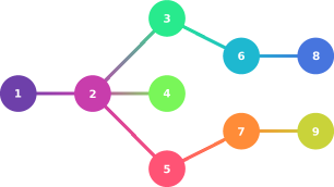
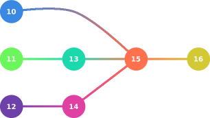
(a) Job 1 with 9 operations		(b) Job 2 with 7 operations

Figure 1: Directed acyclic graph representing precedence constraints between operations of two different jobs with $9$ and $7$ operations, respectively. Nodes represent operations and arcs, directed from left to right, represent precedence constraints. Operations are numbered consecutively from $1$ to $16$. So, $V=\{1,2,\dots,16\}$ and $A=\{(1,2),(2,3),(2,4),(2,5),(3,6),(5,7),(6,8),(7,9),(10,15),(11,13),(12,14),(13,15),(14,15),(15,16)\}$.

Machines $k=1,\dots,m$ have periods of unavailability given by $[\underline{u}^{k}_{1},\bar{u}^{k}_{1}],\dots,[\underline{u}^{k}_{q_{k}},\bar{u}^{k}_{q_{k}}]$, where $q_{k}$ is the number of unavailability periods of machine $k$. Although preemption is not allowed, the execution of an operation can be interrupted by periods of unavailability of the machine to which it was assigned; i.e., operations are resumable. The starting time $s_{i}$ of an operation $i$ assigned to a machine $\kappa(i)$ must be such that $s_{i}\notin[\underline{u}^{\kappa(i)}_{\ell},\bar{u}^{\kappa(i)}_{\ell})$ for all $\ell=1,\dots,q_{\kappa(i)}$. This means that the starting time may coincide with the end of a period of unavailability (the possible existence of a non-null setup time is being ignored here), but it cannot coincide with its beginning nor belong to its interior, since these two situations would represent a fictitious prior starting time. In an analogous way, the completion time $c_{i}$ must be such that $c_{i}\notin(\underline{u}^{\kappa(i)}_{\ell},\bar{u}^{\kappa(i)}_{\ell}]$ for all $\ell=1,\dots,q_{\kappa(i)}$, since violating these constraints would correspond to allowing a fictitious delayed completion time. It is clear that if operation $i$ is completed at time $c_{i}$ and $c_{i}\in(\underline{u}^{\kappa(i)}_{\ell},\bar{u}^{\kappa(i)}_{\ell}]$ for some $\ell$ then it is because the operation is actually completed at instant $\underline{u}^{\kappa(i)}_{\ell}$; see Figure 2.

(a)
(b)	(c)

Figure 2: Allowed and forbidden relations between the starting time $s_{i}$, the completion time $c_{i}$, and the periods of unavailability of machine $\kappa(i)$. In (a), allowed positions are illustrated. For further reference, it is worth mentioning that the sum of the sizes of the two periods of unavailability in between $s_{i}$ and $c_{i}$ is named $u_{i}$; so the relation $s_{i}+p_{i,\kappa(i)}+u_{i}=c_{i}$ holds. The top picture in (b) shows the forbidden situation $s_{i}\in[\underline{u}^{\kappa(i)}_{\ell},\bar{u}^{\kappa(i)}_{\ell})$ for some $\ell$, that corresponds to a fictitious prior starting time. The valid value for $s_{i}$ that corresponds to the same situation is illustrated in the bottom picture in (b). The top picture in (c) shows a forbidden situation in which $c_{i}\in(\underline{u}^{\kappa(i)}_{\ell},\bar{u}^{\kappa(i)}_{\ell}]$ for some $\ell$, that corresponds to a fictitious delayed completion time. The valid value for $c_{i}$ that corresponds to the same situation is illustrated in the bottom picture in (c).

The precedence relations $(i,j)\in A$ have a special meaning in the OPS scheduling problem. Each operation $i$ has a constant $\theta_{i}\in(0,1]$ associated with it. On the one hand, the precedence relation means that operation $j$ can start to be processed after $\lceil\theta_{i}\times p_{ik}\rceil$ units of time of operation $i$ have already been processed, where $k\in F(i)$ is the machine to which operation $i$ has been assigned. We assume that the given value of $\theta_{i}$ is such that the ongoing processing of operation $i$ does not prevent the regular processing of operation $j$. (This assumption holds in the real-world instances of the OPS scheduling problem. However, aiming to increase the potential benefit of the overlapping, constants $\theta_{i}$ ($i\in V$) could be easily substituted with constants $\theta_{i,\kappa(i),j,\kappa(j)}$ ($(i,j)\in A$, $\kappa(i)\in F(i)$, $\kappa(j)\in F(j)$). On the other hand, the precedence relation imposes that operation $j$ cannot be completed before the completion of operation $i$. See Figure 3. In the figure, for a generic operation $h$ assigned to machine $\kappa(h)$, $\bar{c}_{h}$ denotes the instant at which $\lceil\theta_{h}\times p_{h,\kappa(h)}\rceil$ units of time of operation $h$ have already been processed. Note that $\bar{c}_{h}$ could be larger than $s_{h}+\lceil\theta_{h}\times p_{h,\kappa(h)}\rceil$ due to the machines’ periods of unavailability.

Figure 3: According to the DAG in the right-hand-side of Figure 1, we have $(10,15)$, $(13,15)$, and $(14,15)\in A$. This means that $s^{\mathrm{lb}}_{15}=\max\{\bar{c}_{10},\bar{c}_{13},\bar{c}_{14}\}$ is a lower bound for the starting time $s_{15}$; while $c^{\mathrm{lb}}_{15}=\max\{c_{10},c_{13},c_{14}\}$ is a lower bound for the completion time $c_{15}$. If $\kappa(15)=\kappa(13)$ and operation $15$ is sequenced right after operation $13$, then $c_{13}+\gamma^{I}_{13,15,\kappa(15)}$ is another lower bound for $s_{15}$, where $\gamma^{I}_{13,15,\kappa(15)}$ is the sequence-dependent setup time corresponding to the processing of operation $13$ right before operation $15$ on machine $\kappa(15)$. In addition, $s_{15}$ must also satisfy $s_{15}\geq r_{15}$.

Operations have a sequence-dependent setup time associated with them. If the execution of operation $j$ on machine $k$ is immediately preceded by the execution of operation $i$, then its associated setup time is given by $\gamma^{I}_{ijk}$ (the super-index “I” stands for intermediate or in between); while, if operation $j$ is the first operation to be executed on machine $k$, the associated setup time is given by $\gamma^{F}_{jk}$ (the super-index “F” stands for first). Of course, setup times of the form $\gamma^{F}_{jk}$ are defined if and only if $k\in F(j)$ while setup times of the form $\gamma^{I}_{ijk}$ are defined if and only if $k\in F(i)\cap F(j)$. Unlike the execution of an operation, the execution of a setup operation cannot be interrupted by periods of unavailability of the corresponding machine, i.e., setup operations are non-resumable. Moreover, the completion time of the setup operation must coincide with the starting time of the associated operation; see Figure 4.

Figure 4: Illustration of the fact that, unlike the processing of a regular operation, a setup operation cannot be interrupted by periods of unavailability of the machine to which the operation has been assigned. The picture also illustrates that the completion time of the setup operation must coincide with the starting time of the operation itself. In the picture, it is assumed that operation $i$ is the first operation to be executed on machine $\kappa(i)$; thus, the duration of its setup operation is given by $\gamma^{F}_{i,\kappa(i)}$.

Finally, the OPS scheduling problem may have some operations that were already assigned to a machine and for which the starting time has already been defined. These operations are known as fixed operations. Note that the setup time of the operations is sequence-dependent. Then, the setup time of a fixed operation is unknown and it depends on which operation (if any) will precede the execution of the fixed operation in the machine to which it was assigned. Let $T\subseteq V$ be the set of indices of the fixed operations. Therefore, we assume that for $i\in T$, $s_{i}$ is given and that $F(i)$ is a singleton, i.e., $F(i)=\{k_{i}\}$ for some $k_{i}\in\{1,2,\dots,m\}$. Since a fixed operation $i$ has already been assigned to a machine $k_{i}$, its processing time $p_{i}=p_{i,k_{i}}$ is known. Moreover, the instant $\bar{c}_{i}$ that is the instant at which $\lceil\theta_{i}\times p_{i}\rceil$ units of time of its execution has already been processed, its completion time $c_{i}$, and the value $u_{i}$ such that $s_{i}+u_{i}+p_{i}=c_{i}$ can be easily computed taking the given starting time $s_{i}$ and the periods of unavailability of machine $k_{i}$ into account. It is assumed that, if $i\in T$ and $(j,i)\in A$, then $j\in T$, i.e., predecessors of fixed operations are fixed operations as well. This assumption is not present in the MILP formulation of the problem introduced in Lunardi et al. (2020a). However, it is a valid assumption in practical instances of the problem; and assuming it holds eliminates the existence of infeasible instances and simplifies the development of a solution method. For further reference, we define $\bar{o}=|V|-|T|$, i.e., $\bar{o}$ is the number of non-fixed operations.

The problem, therefore, consists of assigning the non-fixed operations to the machines and sequencing all the operations while satisfying the given constraints. The objective is to minimize the makespan. Mixed integer linear programming and constraint programming models for the problem were given in Lunardi et al. (2020a).

4 Representation scheme and construction of a feasible solution

In this section, we describe (a) the way the assignment of non-fixed operations to machines is represented, (b) the way the sequence of non-fixed operations assigned to each machine is represented and (c) the way a feasible solution is constructed from these two representations. From now on, we assume that all numbers that define an instance of the OPS scheduling problem are integer numbers. Namely, we assume that the processing times $p_{ik}$ ($i\in V$, $k\in F(i)$), the release times $r_{i}$ ($i\in V$), the beginning $\underline{u}^{k}_{\ell}$ and end $\bar{u}^{k}_{\ell}$ of every period of unavailability of every machine ($k=1,\dots,m$, $\ell=1,\dots,q_{k}$), the setup times $\gamma^{F}_{jk}$ ($j\in V$, $k\in F(j)$) and $\gamma^{I}_{ijk}$ ($i,j\in V$, $k\in F(i)\cap F(j)$), and the starting times $s_{i}$ of every fixed operation $i\in T$ are integer values. It is very natural to assume that these constants are rational numbers; and the integrality can be easily obtained with a change of units.

4.1 Representation of the assignment of non-fixed operations to machines

Let $\{i_{1},i_{2},\dots,i_{\bar{o}}\}=V\setminus T$, with $i_{1}\leq i_{2}\leq\dots\leq i_{\bar{o}}$, be the set of non-fixed operations. For each $i_{j}$, let $K_{i_{j}}=(k_{i_{j},1},k_{i_{j},2},\dots,k_{i_{j},|F(i_{j})|})$ be a permutation of $F(i_{j})$. Let ${\tilde{\pi}=(\tilde{\pi}_{j}\in[0,1):j\in\{1,\dots,\bar{o}\})}$ be an array of real numbers that encodes the machine $k_{i_{j},\pi_{j}}$ to which each non-fixed operation $i_{j}$ is assigned, where

$$\pi_{j}=\left\lfloor\tilde{\pi}_{j}|F(i_{j})|+1\right\rfloor,$$ (1)

for $j=1,\dots,\bar{o}$. For example, given $F(i_{j})=\{1,4,7\}$, the permutation $K_{i_{j}}=(1,4,7)$, and $\tilde{\pi}_{j}=0.51$, we have $\pi_{j}=\lfloor 0.51\times 3+1\rfloor=2$, and, thus, $k_{i_{j},\pi_{j}}=k_{i_{j},2}=4$; implying that operation $i_{j}$ is assigned to machine 4. For simplicity, we denote $\kappa(i_{j})=\kappa_{i_{j},\pi_{j}}$. Then, if we define $\kappa(i)$ as the only element in the singleton $F(i)$ for the fixed operations $i\in T$, it becomes clear that the array of real numbers $\tilde{\pi}=(\tilde{\pi}_{1},\dots,\tilde{\pi}_{\bar{o}})$ defines a machine assignment $i\rightarrow\kappa(i)$ for $i=1,\dots,o$; see Figure 5.

$j$	1	2	3	4	5	6	7	8	9	10	11	12	13	14
$i_{j}$	2	3	4	5	6	7	8	9	10	12	13	14	15	16
$K_{i_{j}}$	$(1,2)$	$(3,4)$	$(2,4)$	$(2,4)$	$(1,2)$	$(1,3)$	$(3,4)$	$(1,2)$	$(3,4)$	$(1,3)$	$(1,3)$	$(1,2)$	$(2,4)$	$(1,3)$
$\tilde{\pi}_{j}$	0.05	0.79	0.48	0.26	0.17	0.53	0.99	0.09	0.95	0.63	0.52	0.02	0.31	0.62
$\pi_{j}$	1	2	1	1	1	2	2	1	2	2	2	1	1	2
$\kappa(i_{j})$	1	4	2	2	1	3	4	1	4	3	3	1	2	3

Figure 5: An arbitrary machine assignment array assuming that operations $1$ and $11$ are fixed operations with $F(1)=\{3\}$ and $F(11)=\{2\}$, so $\kappa(1)=3$ and $\kappa(11)=2$.

4.2 Representation of a sequencing of the non-fixed operations

Let $\tilde{\sigma}=(\tilde{\sigma}_{j}\in[0,1):j\in\{1,\dots,\bar{o}\})$ be an array of real numbers that encodes the order of execution of the non-fixed operations that are assigned to the same machine. Consider two non-fixed operations $i_{a}$ and $i_{b}$ such that $\kappa(i_{a})=\kappa(i_{b})$, i.e., that were assigned to the same machine. If $\tilde{\sigma}_{a}<\tilde{\sigma}_{b}$ (or $\tilde{\sigma}_{a}=\tilde{\sigma}_{b}$ and $i_{a}<i_{b}$) and if there is no path from $i_{b}$ to $i_{a}$ in the DAG $(V,A)$, then operation $i_{a}$ is executed before operation $i_{b}$; otherwise $i_{b}$ is executed before $i_{a}$.

Let $\sigma=(\sigma_{j}:j\in\{1,\dots,\bar{o}\})$ be a permutation of the set of non-fixed operations $\{i_{1},\dots,i_{\bar{o}}\}$ such that, for every pair of non-fixed operations $\sigma_{j_{1}}$ and $\sigma_{j_{2}}$ with $\kappa(\sigma_{j_{1}})=\kappa(\sigma_{j_{2}})$, we have that $j_{1}<j_{2}$ if and only if $\sigma_{j_{1}}$ is processed before $\sigma_{j_{2}}$. The permutation $\sigma$ can be computed from $\tilde{\sigma}$ and the DAG $(V,A)$ as follows: (i) start with $\ell\leftarrow 0$; (ii) let $R\subseteq\{i_{1},i_{2},\dots,i_{\bar{o}}\}$ be the set of non-fixed operations $i_{j}$ such that $i_{j}\neq\sigma_{s}$ for $s=1,\dots,\ell$ and, in addition, for every arc $(i,i_{j})\in A$ we have $i\in V\setminus T$ and $i=\sigma_{t}$ for some $t=1,\dots,\ell$ or $i\in T$; (iii) take the operation $i_{j}\in R$ with smallest $\tilde{\sigma}_{j}$ (in case of a tie, select the operation with the smallest index $i_{j}$), set $\sigma_{\ell+1}=i_{j}$, and $\ell\leftarrow\ell+1$; and (iv) if $\ell<\bar{o}$, return back to (ii). See Figure 6.

For further reference, for each machine $k$ we define $\phi_{k}=(\phi_{k,1},\dots,\phi_{k,|\phi_{k}|})$ as the subsequence of $\sigma$ composed of the operations $\sigma_{\ell}$ such that $\kappa(\sigma_{\ell})=k$. Given the machine assignment $\tilde{\pi}$ as illustrated in Figure 5 and the order of execution within each machine implied by $\tilde{\sigma}$ as illustrated in Figure 6, we have $\phi_{1}=(2,14,6,9),\phi_{2}=(5,15,4),\phi_{3}=(12,13,7,16)$, and $\phi_{4}=(10,3,8)$. Note that fixed operations are not included. Moreover, we define $\Phi=(\phi_{1},\dots,\phi_{m})$.

$j$	1	2	3	4	5	6	7	8	9	10	11	12	13	14
$i_{j}$	2	3	4	5	6	7	8	9	10	12	13	14	15	16
$\tilde{\sigma}_{j}$	0.05	0.55	0.95	0.51	0.75	0.54	0.00	0.99	0.15	0.15	0.16	0.11	0.79	0.55
$\sigma_{j}$	2	10	12	14	13	5	7	3	6	8	15	16	4	9

Figure 6: An operations execution order sequence $\sigma$ produced by considering the values in $\tilde{\sigma}$ and the precedence relations given by the DAG represented in Figure 1. Note, once again, that fixed operations $1$ and $11$ are unsequenced at this point.

4.3 Construction of a feasible solution and calculation of the makespan

Let the machine assignment $\tilde{\pi}$ and the execution order $\tilde{\sigma}$ be given; and let $\pi$, $\sigma$, $\kappa$, and $\phi_{k}$ ($k=1,\dots,m$) be computed from $\tilde{\pi}$ and $\tilde{\sigma}$ as described in Sections 4.1 and 4.2. Recall that, for all fixed operations $i\in T$, it is assumed that we already know the starting time $s_{i}$, the processing time $p_{i}$, the completion time $c_{i}$, the value $u_{i}$ such that $s_{i}+u_{i}+p_{i}=c_{i}$, and the “partial completion time” $\bar{c}_{i}$, that is the instant at which $\lceil\theta_{i}\times p_{i}\rceil$ units of time of operation $i$ have already been processed. We now describe an algorithm to compute $s_{i}$, $\bar{c}_{i}$, $u_{i}$, $p_{i}$, and $c_{i}$ for all $i\in V\setminus T$ and to sequence the fixed operations $i\in T$ in order to construct a feasible schedule. The algorithm also determines for all the operations (fixed and non-fixed) the corresponding sequence-dependent setup time $\xi_{i}$ and some additional quantities ($d_{i}$, $s_{i}^{\mathrm{lb}}$, and $c_{i}^{\mathrm{lb}}$) whose meaning will be elucidated later. The algorithm processes one non-fixed operation $i\in V\setminus T$ at a time and schedules it as soon as possible (for the given $\tilde{\pi}$ and $\tilde{\sigma}$), constructing a semi-active schedule. This computation includes sequencing the fixed operations $i\in T$.

Define $\mathrm{pos}(i)$ as the position of operation $i$ in the sequence $\phi_{\kappa(i)}$; i.e., for any non-fixed operation $i$, we have that $1\leq\mathrm{pos}(i)\leq|\phi_{\kappa(i)}|$. This means that, according to $\tilde{\pi}$ and $\tilde{\sigma}$ and ignoring the fixed operations, for a non-fixed operation $i$, $\mathrm{ant}(i)=\phi_{\kappa(i),\mathrm{pos}(i)-1}$ is the operation that is processed immediately before $i$ on machine $\kappa(i)$; and $\mathrm{ant}(i)=0$ if $i$ is the first operation to be processed on the machine. For further reference, we also define $\mathrm{suc}(i)=\phi_{\kappa(i),\mathrm{pos}(i)+1}$ as the immediate successor of operation $i$ on machine $\kappa(i)$, if operation $i$ is not the last operation to be processed on the machine; and $\mathrm{suc}(i)=o+1$, otherwise.

For $k=1,\dots,m$, define the $(o+1)\times o$ matrices $\Gamma^{k}$ of setup times, with row index starting at $0$, given by $\Gamma^{k}_{0j}=\gamma^{F}_{jk}$ for $j=1,\dots,o$ and $\Gamma^{k}_{ij}=\gamma^{I}_{ijk}$ for $i,j=1,\dots,o$. Then we have that, according to $\phi_{k}$ (that does not include the fixed operations yet), the setup time $\xi_{i}$ of operation $i$ is given by $\xi_{i}=\Gamma^{\kappa(i)}_{\mathrm{ant}(i),i}$. Moreover, if we define $c_{0}=0$, we obtain $c_{\mathrm{ant}(i)}+\xi_{i}$ as a lower bound for the starting time $s_{i}$ of operation $i$ on machine $\kappa(i)$.

The algorithm follows below. In the algorithm, $\mathrm{size}(\cdot)$ is a function that, if applied to an interval $[a,b]$, returns its size given by $b-a$ and, if applied to a set of non-overlapping intervals, returns the sum of the sizes of the intervals.

Algorithm 4.3.1.

Input: $\sigma_{i}$, $\kappa_{i}$ ($i\in V$), $\phi_{k}$ ($k=1,\dots,m$), $s_{i}$, $u_{i}$, $p_{i}$, $\bar{c}$, $c_{i}$ ($i\in T$).

Output: $\phi_{k}$ ($k=1,\dots,m$), $s_{i}$, $u_{i}$, $p_{i}$, $\bar{c}$, $c_{i}$ ($i\in V\setminus T$), $\xi_{i}$, $d_{i}$, $s_{i}^{\mathrm{lb}}$, $c_{i}^{\mathrm{lb}}$ ($i\in V$), $C_{\max}$.

For each $\ell=1,\dots,\bar{o}$, execute Steps 1 to 6. Then execute Step 7.

Step 1:

Set $i\leftarrow\sigma_{\ell}$, $k\leftarrow\kappa(i)$, $p_{i}=p_{ik}$, $\bar{p}_{i}=\lceil\theta_{i}\times p_{ik}\rceil$, and $\operatorname{delay}_{i}\leftarrow 0$ and compute

$$s_{i}^{\mathrm{lb}}=\max\left\{\max_{\{j\in V|(j,i)\in A\}}\left\{\bar{c}_{j}\right\},\;r_{i}\right\}\;\mbox{ and }\;c_{i}^{\mathrm{lb}}=\max_{\{j\in V|(j,i)\in A\}}\left\{c_{j}\right\}.$$ (2)

Step 2:

Set $\xi_{i}=\Gamma^{k}_{\mathrm{ant}(i),i}$, define

$$d_{i}=\max\left\{s_{i}^{\mathrm{lb}},\;c_{\mathrm{ant}(i)}+\xi_{i}\right\},$$ (3)

and compute $s_{i}\geq d_{i}+\operatorname{delay}_{i}$ as the earliest starting time such that the interval $(s_{i}-\xi_{i},s_{i}]$ does not intersect any period of unavailability of machine $k$, i.e.,

$$\left(\cup_{\ell=1}^{q_{k}}[\underline{u}_{\ell}^{k},\bar{u}_{\ell}^{k}]\right)\cap(s_{i}-\xi_{i},s_{i}]=\emptyset.$$ (4)

Step 3:

Compute the completion time $c_{i}\not\in(\underline{u}_{\ell}^{k},\bar{u}_{\ell}^{k}]$, for $\ell=1,\dots,q_{k}$, such that

$$\mathrm{size}([s_{i},c_{i}])-u_{i}=p_{i},$$ (5)

where

$$u_{i}=\mathrm{size}([s_{i},c_{i}]\cap(\cup_{\ell=1}^{q_{k}}[\underline{u}_{\ell}^{k},\bar{u}_{\ell}^{k}]))$$ (6)

is the time machine $k$ is unavailable in between $s_{i}$ and $c_{i}$.

Step 4:

Let $f\in T$ be an operation fixed at machine $k$ such that

$$c_{\mathrm{ant}(i)}\leq s_{f}<c_{i}+\Gamma^{k}_{if}.$$ (7)

If there is none, go to Step 5. If there is more than one, consider the one with the earliest starting time $s_{f}$. Insert $f$ in $\phi_{k}$ in between operations $\mathrm{ant}(i)$ and $i$ and go to Step 2. (Note that this action automatically redefines $\mathrm{ant}(i)$ as $f$.)

Step 5:

If $c_{i}\not\geq c_{i}^{\mathrm{lb}}$ then set $\operatorname{delay}_{i}=\mathrm{size}([c_{i},\hat{c}_{i}^{\mathrm{lb}}])-\mathrm{size}([c_{i},\hat{c}_{i}^{\mathrm{lb}}]\cap\left(\cup_{\ell=1}^{q_{k}}[\underline{u}_{\ell}^{k},\bar{u}_{\ell}^{k}]\right))$, where

$$\hat{c}_{i}^{\mathrm{lb}}=\left\{\begin{array}[]{ll}c_{i}^{\mathrm{lb}},&\mbox{if }c_{i}^{\mathrm{lb}}\not\in(\underline{u}_{\ell}^{k},\bar{u}_{\ell}^{k}]\mbox{ for }\ell=1,\dots,q_{k},\\[5.69054pt] \bar{u}_{\ell}^{k}+1,&\mbox{if }c_{i}^{\mathrm{lb}}\in(\underline{u}_{\ell}^{k},\bar{u}_{\ell}^{k}]\mbox{ for some }\ell\in\{1,\dots,q_{k}\},\end{array}\right.$$

and go to Step 2.

Step 6:

Compute the “partial completion time” $\bar{c}_{i}\not\in(\underline{u}_{\ell}^{k},\bar{u}_{\ell}^{k}]$, for $\ell=1,\dots,q_{k}$, such that $\mathrm{size}([s_{i},\bar{c}_{i}])-\bar{u}_{i}=\bar{p}_{i}$, where $\bar{u}_{i}=\mathrm{size}([s_{i},\bar{c}_{i}]\cap(\cup_{\ell=1}^{q_{k}}[\underline{u}_{\ell}^{k},\bar{u}_{\ell}^{k}]))$.

Step 7:

Compute $C_{\max}=\max_{i\in V}\{c_{i}\}$. For each unsequenced operation $f\in T$, sequence it according to its starting time $s_{f}$, update $\phi_{\kappa(f)}$, compute $s_{f}^{\mathrm{lb}}$ and $c_{f}^{\mathrm{lb}}$ according to (2), $\xi_{f}=\Gamma_{\mathrm{ant}(f)}^{\kappa(f)}$, and $d_{f}$ as in (3).

At Step 1, a lower bound $s_{i}^{\mathrm{lb}}$ to $s_{i}$ is computed based on the release time $r_{i}$ and the partial completion times $\bar{c}_{j}$ of the operations $j$ such that $(j,i)\in A$ exists. In an analogous way, a lower bound $c_{i}^{\mathrm{lb}}$ to $c_{i}$ is computed, based on the completion times $c_{j}$ of the operations $j$ such that $(j,i)\in A$ exists.

At Step 2, a tentative $s_{i}$ is computed. At this point, it is assumed that the operation which is executed immediately before $i$ on machine $\kappa(i)$ is the one that appears right before it in $\phi_{k}$ (namely $\mathrm{ant}(i)$); and, for this reason, it is considered that the setup time of operation $i$ is given by $\xi_{i}=\Gamma^{k}_{\mathrm{ant}(i),i}$. (This may not be the case if it is decided that a still-unsequenced fixed operation should be sequenced in between them.) The computed $s_{i}$ is required by (3) to be not smaller than (a) its lower bound $s_{i}^{\mathrm{lb}}$ computed at Step 1 and (b) the completion time $c_{\mathrm{ant}(i)}$ of operation $\mathrm{ant}(i)$ plus the setup time $\xi_{i}$. Note that if operation $i$ is the first operation to be processed on machine $\kappa(i)$ then $\mathrm{ant}(i)=0$ and, by definition, $c_{\mathrm{ant}(i)}=c_{0}=0$. At this point, we assume that $\operatorname{delay}_{i}=0$. Its role will be elucidated soon. In addition to satisfying the lower bounds (a) and (b), $s_{i}$ is required in (4) to be such that (i) it does not coincide with the beginning of a period of unavailability, (ii) there is enough time right before $s_{i}$ to execute the setup operation, and (iii) the setup operation is not interrupted by periods of unavailability of the machine. We pick $s_{i}$ as the smallest value that satisfies the lower bounds (a) and (b) and conditions (i), (ii), and (iii) mentioned above. Therefore, it becomes clear that there is only a finite number—in fact, a small number—of possibilities for $s_{i}$ that depends on the imposed lower bounds and the periods of unavailability of the machine.

Once the tentative $s_{i}$ has been computed in Step 2, Step 3 is devoted to the computation of its companion completion time $c_{i}$. Basically, ignoring the possible existence of fixed operations on the machine, (5) and (6) indicate that $c_{i}$ is such that between $s_{i}$ and $c_{i}$ the time during which machine $\kappa(i)$ is available is exactly the time required to process operation $i$. In addition, $c_{i}\not\in(\underline{u}_{\ell}^{k},\bar{u}_{\ell}^{k}]$, for $\ell=1,\dots,q_{k}$, says that, if the duration of the interval yields $c_{i}\in[\underline{u}_{\ell}^{k},\bar{u}_{\ell}^{k}]$ for some $\ell\in\{1,\dots,q_{k}\}$, we must take $c_{i}=\underline{u}_{\ell}^{k}$, since any other choice would artificially increase the completion time of the operation.

In Step 4 it is checked whether the selected interval $[s_{i},c_{i}]$ is infeasible due to the existence of a fixed operation on the machine. If there is not a fixed operation $f$ satisfying (7) then Step 4 is skipped. Note that $c_{\mathrm{ant}(i)}$ is the completion time of the last operation scheduled on machine $\kappa(i)$. This means that if a fixed operation $f$ exists such that $s_{f}\geq c_{\mathrm{ant}(i)}$, the fixed operation $f$ is still unsequenced. The non-existence of a fixed operation $f$ satisfying (7) is related to exactly one of the following two cases: (a) there are no fixed operations on machine $\kappa(i)$ or all fixed operations on machine $\kappa(i)$ have already been sequenced; and (b) the starting time $s_{f}$ of the closest unsequenced fixed operation $f$ on machine $\kappa(i)$ is such that operation $i$ can be scheduled right after operation $\mathrm{ant}(i)$, starting at $s_{i}$, being completed at $c_{i}$ and, after $c_{i}$ and before $s_{f}$ there is enough time to process the setup operation with duration $\Gamma^{\kappa(i)}_{if}$. Assume now that at least one fixed operation satisfying (7) exists and let $f$ be the one with smallest $s_{f}$. This means that to schedule operation $i$ in the interval $[s_{i},c_{i}]$ is infeasible; see Figure 7. Therefore, operation $f$ must be sequenced right after $\mathrm{ant}(i)$, by including it in $\phi_{\kappa(i)}$ in between $\mathrm{ant}(i)$ and $i$. This operation transforms $f$ in a sequenced fixed operation that automatically becomes $\mathrm{ant}(i)$, i.e., the operation sequenced on machine $\kappa(i)$ right before operation $i$. With the redefinition of $\mathrm{ant}(i)$, the task of determining the starting and the completion times of operation $i$ must be restarted. This task restarts returning to Step 2, where a new setup time for operation $i$ is computed and a new $c_{\mathrm{ant}(i)}$ is considered in (3). Since the number of fixed operations is finite and the number of unsequenced fixed operations is reduced by one, this iterative process ends in a finite amount time.

Figure 7: If a fixed operation $f$ on machine $\kappa(i)$ exists such that $c_{\mathrm{ant}(i)}\leq s_{f}<c_{i}+\Gamma^{\kappa(i)}_{if}$, it means that there is not enough space for operation $i$ after $\mathrm{ant}(i)$ and before $f$. Thus, the unsequenced fixed operations $f$ must be sequenced in between operations $\mathrm{ant}(i)$ and $i$.

Step 5 is devoted to checking whether the computed completion time $c_{i}$ is smaller than its lower bound $c_{i}^{\mathrm{lb}}$, computed at Step 1, or not. If $c_{i}\geq c_{i}^{\mathrm{lb}}$, the algorithm proceeds to Step 6. In case $c_{i}<c_{i}^{\mathrm{lb}}$, the starting time of operation $i$ must be delayed. This is the role of the variable $\operatorname{delay}_{i}$ that was initialized with zero. If the extent of the delay is too short, the situation may repeat. If the extent is too long, the starting of the operation may be unnecessarily delayed. Figure 8 helps to visualize that the time during which machine $\kappa(i)$ is available in between $c_{i}$ and $c_{i}^{\mathrm{lb}}$ is the minimum delay that is necessary to avoid the same situation when a new tentative $s_{i}$ and its associated $c_{i}$ are computed. So, the delay is computed and a new attempt is done by returning to Step 2; this time with a non-null $\operatorname{delay}_{i}$.

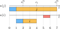
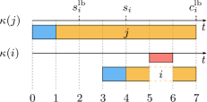
(a)	(b)
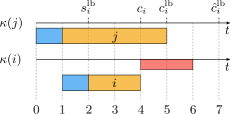
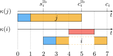
(c)	(d)

Figure 8: Delay computation for the case in which $c_{i}\not\geq c_{i}^{\mathrm{lb}}$. In case (a), $\hat{c}_{i}^{\mathrm{lb}}=c_{i}^{\mathrm{lb}}$ and machine $\kappa(i)$ has two units of available time in between $c_{i}$ and $c_{i}^{\mathrm{lb}}$. Adding this delay to the lower bound of $s_{i}$ results in the feasible schedule (of operation $i$) depicted in (b). In case (c), $c_{i}^{\mathrm{lb}}\in(\underline{u}_{\ell}^{\kappa(i)},\bar{u}_{\ell}^{\kappa(i)}]\mbox{ for some }\ell\in\{1,\dots,q_{\kappa(i)}\}$. Thus, $\hat{c}_{i}^{\mathrm{lb}}=\bar{u}_{\ell}^{\kappa(i)}+1$. Machine $\kappa(i)$ has one unit of available time in between $c_{i}$ and $\hat{c}_{i}^{\mathrm{lb}}$. Adding this delay to the lower bound of $s_{i}$ results in the feasible schedule (of operation $i$) depicted in (d).

When the algorithm arrives at Step 6, feasible values for $s_{i}$ and $c_{i}$ have been computed and we simply compute the partial completion time $\bar{c}_{i}$ that will be used for computing the starting and completion times of the forthcoming operations.

While executing Steps 1–6 for $\ell=1,\dots,\bar{o}$, i.e., while scheduling the unfixed operations, some fixed operations have to be sequenced as well. However, when the last unfixed operation is scheduled, it may be the case that some fixed operations, that were scheduled “far after” the largest completion time of the unfixed operations, played no role in the scheduling process and thus remain unsequenced, i.e., these fixed operations are not in $\phi_{k}$ for any $k$. These unsequenced fixed operations are sequenced in Step 7.

5 Local search

Given an initial solution, a local search procedure is an iterative process that constructs a sequence of solutions in such a way that each solution in the sequence is in the neighborhood of its predecessor in the sequence. The neighborhood of a solution is given by all solutions obtained by applying a movement to the solution. A movement is a simple modification of a solution. In addition, the local search described in the current section is such that each solution in the sequence improves the objective function value of its predecessor. In the remainder of the current section, the neighbourhood and the movement introduced in Mastrolilli and Gambardella (2000) for the FJS are extended to deal with the OPS scheduling problem.

The definition of the proposed movement is based on the representation of a solution by a digraph. Let $\tilde{\pi}$, encoding the machine assignment of the non-fixed operations, and $\tilde{\sigma}$, encoding the order of execution of the non-fixed operations within each machine, be given. Moreover, assume that, using Algorithm 4.3.1, $\xi_{i}$, $d_{i}$, $s_{i}$, $u_{i}$, $p_{i}$, $\bar{c}_{i}$, $c_{i}$, $s_{i}^{\mathrm{lb}}$, $c_{i}^{\mathrm{lb}}$, and $d_{i}$ have been computed for all $i=1,\dots,o$. From now on, $\varsigma(\tilde{\pi},\tilde{\sigma})=(\tilde{\pi},\tilde{\sigma},\pi,\sigma,\kappa,\Phi,\xi,d,s,u,p,\bar{c},c,s^{\mathrm{lb}},c^{\mathrm{lb}})$ represents a feasible solution. (Recall that $\pi$ is computed from $\tilde{\pi}$ as defined in (1); $\sigma$ and $\Phi$ are computed from $\tilde{\sigma}$ as described in Section 4.2; and $\kappa(i)=\kappa_{i,\pi_{i}}$.) Let $\mathrm{suc}(i)=\phi_{\kappa(i),\mathrm{pos}(i)+1}$ be the successor of operation $i$ on machine $\kappa(i)$, if operation $i$ is not the last operation to be processed on the machine; and $\mathrm{suc}(i)=o+1$, otherwise. Recall that we already defined $\mathrm{ant}(i)=\phi_{\kappa(i),\mathrm{pos}(i)-1}$, if $i$ is not the first operation to be processed on machine $\kappa(i)$; while $\mathrm{ant}(i)=0$, otherwise. This means that, for any $i\in V$, i.e., including non-fixed and fixed operations, $\mathrm{ant}(i)$ and $\mathrm{suc}(i)$ represent, respectively, the operations that are processed right before $i$ (antecedent) and right after $i$ (sucessor) on machine $\kappa(i)$.

The weighted augmented digraph that represents the feasible solution $\varsigma$ is given by $D(\varsigma)=(V\cup\{0,o+1\},A\cup W\cup U)$, where $W=\left\{(\phi_{k,\ell-1},\phi_{k,\ell})\;|\;k\in\{1,\dots,m\}\mbox{ and }\ell\in\{2,...,|\phi_{k}|\}\right\}$ and $U$ is the set of arcs of the form $(0,i)$ for every $i\in V$ such that $\mathrm{ant}(i)=0$ plus arcs of the form $(i,o+1)$ for every $i\in V$ such that $\mathrm{suc}(i)=o+1$; see Figure 9. The weights on the nodes and arcs of $D(\varsigma)$ are defined as follows: (a) arcs $(j,i)\in A$ have weight $\bar{c}_{j}-c_{j}$; (b) arcs $(\mathrm{ant}(i),i)\in W$ have weight $\xi_{i}$; (c) arcs $(0,i)\in U$ have weight $\max\{r_{i},\xi_{i}\}$; (d) arcs $(i,o+1)\in U$ have null weight; (e) each node $i\in V$ has weight $s_{i}-d_{i}+u_{i}+p_{i}$; (f) nodes $0$ and $o+1$ have null weight.

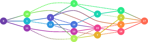
Figure 9: Directed acyclic graph $D(\varsigma)=(V\cup\{0,o+1\},A\cup W\cup U)$ associated with the original precedence relations (in solid lines) illustrated in Figure 1 plus the precedence relations implied by the machine assignment $\tilde{\pi}$ in Figure 5 and the order of execution within each machine implied by $\tilde{\sigma}$ in Figure 6 (dashed lines). Arcs are directed from left to right.

Weights of nodes and arcs are defined in such a way that, if we define the weight of a path $i_{1},i_{2},\dots,i_{q}$ as the sum of the weights of nodes $i_{2},i_{3},\dots,i_{q}$ plus the sum of the weights of arcs $(i_{1},i_{2}),\dots,(i_{q-1},i_{q})$, then the value of the completion time $c_{i}$ of operation $i$ is given by some longest path from node $0$ to node $i$. (If in between two nodes $a$ and $b$ there is more than one arc then the arc with the largest weight must be considered. This avoids naming the arcs explicitly when mentioning a path.) It follows that the weight of some longest path from $0$ to $o+1$ equals $C_{\max}$ and the nodes on this path are called critical nodes or critical operations. We define $t_{i}$ as the weight of a longest path from node $i$ to node $o+1$. The value $t_{i}$ (so-called tail time) gives a lower bound on the time elapsed between $c_{i}$ and $C_{\max}$. It is worth noticing that (a) if an operation $i$ is critical then $c_{i}+t_{i}=C_{\max}$ and that (b) if there is a path from $i$ to $j$ then $t_{i}\geq t_{j}$.

Assume that $\sigma^{\mathrm{ifo}}$ (“ifo” stands for “including fixed operations”) is a permutation of $\{1,2,\dots,o\}$ that represents the order in which operations (non-fixed and fixed) where scheduled by Algorithm 4.3.1. This means that non-fixed operations have in $\sigma^{\mathrm{ifo}}$ the same relative order they have in $\sigma$ and that $\sigma^{\mathrm{ifo}}$ corresponds to $\sigma$ with the fixed operations inserted in the appropriate places. Note that $\sigma^{\mathrm{ifo}}$ can be easily obtained with a simple modification of Algorithm 4.3.1: start with $\sigma^{\mathrm{ifo}}$ as an empty list and every time an operation (non-fixed or fixed) is scheduled, add $i$ to the end of the list. We now describe a simple way to compute $t_{i}$ for all $i\in V\cup\{0,o+1\}$. Define $c_{o+1}=C_{\max}$ and $t_{o+1}=0$ and for $\ell=o,\dots,1$, i.e., in decreasing order, define $i=\sigma^{\mathrm{ifo}}_{\ell}$ and

$$t_{i}=\max\left\{t_{\mathrm{suc}(i)}+\omega(\mathrm{suc}(i))+\omega(i,\mathrm{suc}(i)),\max_{\{j\in V|(i,j)\in A\}}\left\{t_{j}+\omega(j)+\omega(i,j)\right\}\right\},$$ (8)

where $\omega(\cdot)$ and $\omega(\cdot,\cdot)$ represent the weight of a node or an arc, respectively. Finish defining

$$t_{0}=\max_{\{j\in V|(0,j)\in U\}}\left\{t_{j}+\omega(j)+\omega(0,j)\right\}.$$ (9)

In addition to the tail times, the local search strategy also requires identifying a longest (critical) path from node $0$ to node $o+1$, since operations on that path are the critical operations whose reallocation will be attempted. A critical path can be obtained as follows. Together with the computation of (8), define $\mathrm{next}(i)$ as the index in $\{\mathrm{suc}(i)\}\cup\{j\;|\;(i,j)\in A\}$ such that $t_{i}=t_{\mathrm{next}(i)}+\omega(\mathrm{next}(i))+\omega(i,\mathrm{next}(i))$, i.e., the one that realizes the maximum. Analogously, together with (9) define $\mathrm{next}(0)=\operatorname*{argmax}_{\{j\in V|(0,j)\in A\}}\left\{t_{j}+\omega(0,j)\right\}$. A longest path is then given by $0$, $\mathrm{next}(0)$, $\mathrm{next}(\mathrm{next(0)})$, $\mathrm{next}(\mathrm{next}(\mathrm{next(0)}))$, $\dots,$ $o+1$.

5.1 Movement: Reallocating operations

Let $i$ be a (non-fixed) operation to be removed and reallocated. It can be reallocated in the same machine $\kappa(i)$, but in a different position in the sequence, or in a different machine $k\in F(i)$, $k\neq\kappa(i)$. Removing $i$ from $\kappa(i)$ implies removing arcs $(\phi_{\kappa(i),\mathrm{pos}(i)-1},i)$ and $(i,\phi_{\kappa(i),\mathrm{pos}(i)+1})$ from $W\cup U$ and including the arc $(\phi_{\kappa(i),\mathrm{pos}(i)-1},\phi_{\kappa(i),\mathrm{pos}(i)+1})$ in $W$ or $U$. (Whether the arcs to be removed or inserted belong to $W$ or $U$ depends on whether $\mathrm{pos}(i)-1=0$, $\mathrm{pos}(i)+1=o+1$, or none of these two cases occur.) In the same sense, reallocating $i$ implies creating two new arcs and deleting an arc. Let $D(\varsigma)^{-i}$ be the digraph after the removal of the critical operation $i$; and let $D(\varsigma)^{+i}$ be the digraph after its reallocation.

The relevant fact in the reallocation of operation $i$ is avoiding the creation of a cycle in $D(\varsigma)^{+i}$, i.e., the construction of a feasible solution. For each $k\in F(i)$, we define the sets of operations $R_{k}=\{j\in\phi_{k}\;|\;\bar{c}_{j}>s_{i}^{\mathrm{lb}}\}$ and $L_{k}=\{j\in\phi_{k}\;|\;t_{j}+u_{j}+p_{j}>C_{\max}-\bar{c}_{i}^{\mathrm{ub}}\}$, where $\bar{c}_{i}^{\mathrm{ub}}=\min_{(i,j)\in A}\{s_{j}\}$ is an upper bound for $\bar{c}_{i}$ and, thus, $C_{\max}-\bar{c}_{i}^{\mathrm{ub}}$ is a lower bound for the time between $\bar{c}_{i}$ and $C_{\max}$. Properties of $R_{k}$ and $L_{k}$ follow:

R1

If $j\in R_{k}$ then $\bar{c}_{j}>s_{i}^{\mathrm{lb}}$. Assume that there is a path from $j$ to $i$ in $D(\varsigma)^{-i}$. By the definition of $s_{i}^{\mathrm{lb}}$, $\bar{c}_{j}>s_{i}^{\mathrm{lb}}$ implies that $(j,i)\not\in A$. Then, in the path from $j$ to $i$, the immediate predecessor of $i$ must be an operation $j^{\prime}\not\in R_{k}$ and such that $(j^{\prime},i)\in A$, i.e., such that $\bar{c}_{j^{\prime}}\leq s_{i}^{\mathrm{lb}}$. Therefore, we must have $\bar{c}_{j}\leq s_{j^{\prime}}<\bar{c}_{j^{\prime}}\leq s_{i}^{\mathrm{lb}}$. Thus, if $j\in R_{k}$ then there is no path from $j$ to $i$ in $D(\varsigma)^{-i}$.

R2

If $j\in\phi_{k}\setminus R_{k}$ then $s_{j}<\bar{c}_{j}\leq s_{i}^{\mathrm{lb}}\leq s_{i}<\bar{c}_{i}$. Therefore, there is no path from $i$ to $j$ in $D(\varsigma)^{-i}$.

L1

If $j\in L_{k}$ then $t_{j}+u_{j}+p_{j}>C_{\max}-\bar{c}_{i}^{\mathrm{ub}}$. If there were a path from $i$ to $j$ in $D(\varsigma)^{-i}$ then $\bar{c}_{i}\leq s_{j}$ and, therefore, the lower bound on the distance between $\bar{c}_{i}$ and $C_{\max}$, given by $C_{\max}-\bar{c}_{i}^{\mathrm{ub}}$, should be greater than or equal to the lower bound of the distance between $s_{j}$ and $C_{\max}$, given by $t_{j}+u_{j}+p_{j}$. Therefore, if $j\in L_{k}$ then there is no path from $i$ to $j$ in $D(\varsigma)^{-i}$.

L2

If $j\in\phi_{k}\setminus L_{k}$ then $C_{\max}-\bar{c}_{i}^{\mathrm{ub}}\geq t_{j}+u_{j}+p_{j}$. Assume that there is a path from $j$ to $i$ in $D(\varsigma)^{-i}$. Then, we must have $s_{j}<s_{i}$ and, since $\theta_{i}>0$ and, in consequence, $s_{i}<\bar{c}_{i}$, it follows that $s_{j}<\bar{c}_{i}$. This means that the distance between $s_{j}$ and $C_{\max}$ is greater than the distance between $\bar{c}_{i}$ and $C_{\max}$. The latter, by definition, is bounded from below by $C_{\max}-\bar{c}_{i}^{\mathrm{ub}}$, i.e., $t_{j}+u_{j}+p_{j}>C_{\max}-\bar{c}_{i}^{\mathrm{ub}}$. Thus, if $j\in\phi_{k}\setminus L_{k}$ then there is no path from $j$ to $i$ in $D(\varsigma)^{-i}$.

Properties R1, R2, L1, and L2 imply that if operation $i$ is reallocated in the sequence of a machine $k\in F(i)$ in a position such that all operations in $L_{k}\setminus R_{k}$ are to the left of $i$ and all operations in $R_{k}\setminus L_{k}$ are to the right of $i$, then this insertion defines a feasible solution, i.e., $D(\varsigma)^{+i}$ has no cycles.

5.2 Neighborhood

It is well known in the scheduling literature that removing and reallocating a non-critical operation does not reduce the makespan of the current solution. Therefore, in the present work, we define as neighborhood of a solution $\varsigma$ the set of (feasible) solutions that are obtained when each critical operation $i$ is removed and reallocated in all possible positions of the sequence of every machine $k\in F(i)$, as described in the previous section. This means that, for each critical operation $i$, we proceed as follows: (i) operation $i$ is removed from machine $\kappa(i)$; (ii) for each $k\in F(i)$, (iia) the sets $R_{k}$ and $L_{k}$ are determined and (iib) operation $i$ is reallocated in the sequence of machine $k$ in every possible position such that all operations in $L_{k}\setminus R_{k}$ are to the left of $i$ and all operations in $R_{k}\setminus L_{k}$ are to the right of $i$. For further reference, the set of neighbours of $\varsigma$ is named ${\cal N}(\varsigma)$.

5.3 Estimation of the makespan of neighbor solutions

Given the sequences $\tilde{\pi}$ and $\tilde{\sigma}$ of the current solution $\varsigma$, computing the sequences $\tilde{\pi}^{\prime}$ and $\tilde{\sigma}^{\prime}$ (as well as $\pi^{\prime}$, $\sigma^{\prime}$, and $\kappa^{\prime}$) associated with a neighbour solution $\varsigma^{\prime}\in{\cal N}(\varsigma)$ is a trivial task. Computing the makespan (together with the quantities $\xi^{\prime}$, $s^{\prime}$, $u^{\prime}$, $p^{\prime}$, $\bar{c}^{\prime}$, $c^{\prime}$, $s^{\mathrm{lb}^{\prime}}$, $c^{\mathrm{lb}^{\prime}}$) associated with $\varsigma^{\prime}$ is also simple, but it requires executing Algorithm 4.3.1, which might be considered an expensive task in this context. Therefore, the selection of a neighbor is based on the computation of an estimation of its associated makespan. In fact, following Mastrolilli and Gambardella (2000), what is used as an estimation of the makespan is an estimation of the length of a longest path from node $0$ to node $o+1$ in $D(\varsigma^{\prime})$ containing the operation that was reallocated to construct $\varsigma^{\prime}$ from $\varsigma$. The exact length of this path is a lower bound on the makespan associated with $\varsigma^{\prime}$.

The estimation of the makespan of a neighbour solution $\varsigma^{\prime}\in{\cal N}(\varsigma)$ obtained by removing and reallocating operation $i$ somewhere in the sequence of machine $k$ is determined as follows. If $L_{k}\cap R_{k}=\emptyset$ then the estimation of the makespan is given by $s_{i}^{\mathrm{lb}}+p_{ik}+C_{\max}-\bar{c}_{i}^{\mathrm{ub}}$. If $L_{k}\cap R_{k}\neq\emptyset$, consider the elements (operations) in $L_{k}\cap R_{k}$ sorted in increasing order of their starting times; and let $\tau:\{1,\dots,|L_{k}\cap R_{k}|\}\rightarrow L_{k}\cap R_{k}$ be such that $s_{\tau(1)}<s_{\tau(2)}<\dots<s_{\tau(|L_{k}\cap R_{k}|)}$ and, in consequence, $t_{\tau(1)}>t_{\tau(2)}>\dots>t_{\tau(|L_{k}\cap R_{k}|)}$. Let $j$ be such that $j=0$ if operation $i$ is being inserted before operation $\tau(1)$ and $1\leq j\leq|L_{k}\cap R_{k}|$ if operation $i$ is being inserted right after operation $\tau(j)$. In this case, the estimation of the makespan is given by

$$p_{ik}+\left\{\begin{array}[]{ll}s_{i}^{\mathrm{lb}}+p_{\tau(1)}+u_{\tau(1)}+t_{\tau(1)},&\mbox{if }j=0,\\ s_{\tau(j)}+p_{\tau(j)}+u_{\tau(j)}+p_{\tau(j+1)}+u_{\tau(j+1)}+t_{\tau(j+1)},&\mbox{if }1\leq j<|L_{k}\cap R_{k}|,\\ s_{\tau(j)}+p_{\tau(j)}+u_{\tau(j)}+C_{\max}-\bar{c}_{i}^{\mathrm{ub}},&\mbox{if }j=|L_{k}\cap R_{k}|.\end{array}\right.$$

These estimations follow very closely those introduced by Mastrolilli and Gambardella (2000) for the FJS, see (Mastrolilli and Gambardella, 2000, §5) for details.

5.4 Local search procedure

The local search procedure starts at a given solution. It identifies all critical operations (operations in the longest path from node $0$ to node $o+1$) and for each critical operation $i$ and each $k\in F(i)$ it computes the estimation of the makespan associated with removing and reallocating operation $i$ in every possible position of the sequence of machine $k$ (as described in the previous sections). The neighbor with the smallest estimation of the makespan is selected and its actual makespan is computed by applying Algorithm 4.3.1. In case this neighbor solution improves the makespan of the current solution, the neighbor solution is accepted as the new current solution and the iterative process continues. Otherwise, the local search stops.

6 Metaheuristics

In this section, we briefly describe the four metaheuristics that we consider. Two of the metaheuristics, namely genetic algorithm (GA) and differential evolution (DE) are populational methods; while the other two, iterated local search (ILS) and tabu search (TS), are trajectory methods. GA and TS were chosen because they are the two most popular metaheuristics applied to the FJS scheduling problem (see (Chaudhry and Khan, 2016, Table 4)). On the other hand, in the last decade DE has been successfully applied to a wide range of complex real-world problems (see for example Damak et al. (2009), Wang et al. (2010), Ali et al. (2012), Tsai et al. (2013), Yuan and Xu (2013)), but its performance in the FJS scheduling problem with sequencing flexibility hasn’t been tested yet. Another reason that reinforces the choice of DE is that preliminary experiments involving other well-known metaheuristics such as artificial bee colony, particle swarm optimization, and grey wolf optimizer showed that DE achieves much better results than the other methods that were tested (Lunardi, 2020). Finally, ILS is considered due to its simplicity of implementation and usage. All metaheuristics are based on the same representation scheme (described in Section 4) and use the same definition of the neighborhood (described in Section 5).

In the current section, we define $\vec{x}\in\mathbb{R}^{2\bar{o}}$ as the concatenation of a machine assignment $\tilde{\pi}$ and an execution order $\tilde{\sigma}$. This means that $\vec{x}_{1},\dots,\vec{x}_{\bar{o}}$ correspond to $\tilde{\pi}_{1},\dots,\tilde{\pi}_{\bar{o}}$; while $\vec{x}_{\bar{o}+1},\dots,\vec{x}_{2\bar{o}}$ correspond to $\tilde{\sigma}_{1},\dots,\tilde{\sigma}_{\bar{o}}$. Given $\vec{x}$ (and the instance constants $s_{i}$, $u_{i}$, $p_{i}$, $\bar{c}_{i}$, and $c_{i}$ for $i\in T$), it is easy to compute $\pi_{i}$, $\sigma_{i}$ ($i\in V\setminus T$), $\kappa_{i}$ ($i\in V$), and $\phi_{k}$ ($k=1,\dots,m$) as described in Sections 4.1 and 4.2; and then the associated makespan $C_{\max}$ using Algorithm 4.3.1. In this section, given $\vec{x}$, we denote $f(\vec{x})=C_{\max}$. Additionally, in the algorithms, the short terms “chosen”, “random” or “randomly chosen” should be interpreted as abbreviations of “randomly chosen with uniform distribution”.

Initial solutions of all methods are constructed in the same way. For each operation $i\in V\setminus T$, the machine $k\in F(i)$ with the lowest processing time is chosen. (For operations $i\in T$, the machine that processes operation $i$ is fixed by definition.) Then, a cost-based breadth-first search (CBFS) algorithm is used to sequence the operations. The costs of each operation are given by a random number in $[0,1]$. At each iteration of the CBFS, a set of eligible operations $\mathcal{E}$ is defined. Operations in $\mathcal{E}$ are those for which their immediate predecessors have already been sequenced. If $|\mathcal{E}|>1$, operations in $\mathcal{E}$ are sequenced in increasing order of their costs; if $|\mathcal{E}|=1$ then the single operation in $\mathcal{E}$ is sequenced. The procedure ends when $\mathcal{E}=\emptyset$ which implies that all operations have been sequenced. In the following subsections, we briefly and schematically describe the main principles of each metaheuristic.

6.1 Differential Evolution

Proposed by Storn and Price (1997) (see also Price et al. (2006) for further references), DE disturbs the current population members, unlike traditional evolutionary algorithms, with a scaled difference of indiscriminately preferred and dissimilar population members. In the basic variant of the DE, at each iteration, a mutant $\vec{v}^{\,i}$ is generated for each solution $\vec{x}^{\,i}$ ($i=1,2,\dots,n_{\mathrm{size}})$ according to

$$\vec{v}^{\,i}=\vec{x}^{\,r_{1}}+\zeta(\vec{x}^{\,r_{2}}-\vec{x}^{\,r_{3}})$$ (10)

where $\zeta$ is a parameter in $(0,2]$, usually less than or equal to 1, and $r_{1},r_{2},r_{3}\in\{1,2,\dots,n_{\mathrm{size}}\}\setminus\{i\}$ are random indices. Note that $n_{\mathrm{size}}\geq 4$ must be fulfilled, since $r_{1},r_{2},r_{3}$ and $i$ must be mutually different. The parameter $\zeta$ controls the amplifications of the differential variation. The basic DE variant with the mutation scheme given by (10) is named DE/rand/1. The second most often used DE variant, denoted DE/best/1 (see Qin et al. (2008)), is also based on (10) but $r_{1}=\operatorname*{argmin}_{i=1,\dots,n_{\mathrm{size}}}\left\{f(\vec{x}^{\,i})\right\}$, i.e., $\vec{x}^{\,r_{1}}$ is the individual with the best fitness value in the population and $r_{2},r_{3}\in\{1,2,\dots,n_{\mathrm{size}}\}\setminus\{i,r_{1}\}$ are random indices. Once the mutant $\vec{v}^{\,i}$ is generated, a trial $\vec{u}^{\,i}$ is formed as

$$\vec{u}^{\,i}_{j}=\left\{\begin{array}[]{ll}\vec{v}^{\,i}_{j}&\mbox{if a random value in }[0,1]\mbox{ is less than or equal to }p_{\mathrm{cro}}\mbox{ or if }j=R(i),\\ \vec{x}^{\,i}_{j}&\mbox{otherwise},\end{array}\right.$$

where $p_{\mathrm{cro}}\in[0,1]$ is a given parameter and $R(i)$ is a randomly chosen index in $\{1,2,\dots,2\bar{o}\}$, which ensures that at least one element of $\vec{v}^{\,i}$ is passed to $\vec{u}^{\,i}$. To decide whether $\vec{u}^{\,i}$ should become a member of the next generation or not, it is compared with $\vec{x}^{\,i}$ using a greedy criterion. If $f(\vec{u}^{\,i})<f(\vec{x}^{\,i})$, then $\vec{u}^{\,i}$ substitutes $\vec{x}^{\,i}$; otherwise $\vec{x}^{\,i}$ is retained. Algorithm 6.1 shows the essential steps of the proposed DE algorithm.

1:Input parameters: $n_{\mathrm{size}}$, $\zeta$, $p_{\mathrm{cro}}$, $\mathrm{variant}$, and $t$.

2:$\mathcal{P}\leftarrow\emptyset$.

3:for $i\leftarrow 1$ to $n_{\mathrm{size}}$ do

4:    Compute a random array of costs $c\in[0,1]^{o}$ and, using CBFS, construct an initial solution $\vec{x}^{\,i}$.

5:    Let $\mathcal{P}\leftarrow\mathcal{P}\cup\{\vec{x}^{\,i}\}$.

6:while time limit $t$ not reached do

7:    for $i\leftarrow 1$ to $n_{\mathrm{size}}$ do

8:         if $\mathrm{variant}=$ DE/rand/1 then

9:             Compute random numbers $r_{1}\neq r_{2}\neq r_{3}\in\{1,2,...,n_{\mathrm{size}}\}\setminus\{i\}$.

10:         else if $\mathrm{variant}=$ DE/best/1 then

11:             Let $r_{1}\leftarrow\operatorname*{argmin}_{\ell=1,\dots,n_{\mathrm{size}}}\left\{f(\vec{x}^{\,\ell})\right\}$

12:             Compute random numbers $r_{2}\neq r_{3}\in\{1,2,...,n_{\mathrm{size}}\}\setminus\{i,r_{1}\}$.          

13:         Compute $\vec{v}\leftarrow\max\left\{0,\min\left\{\vec{x}^{\,r_{1}}+\zeta(\vec{x}^{\,r_{2}}-\vec{x}^{\,r_{3}}),1-10^{-16}\right\}\right\}$.

14:         Compute a random number $R(i)\in\{1,\dots,2\bar{o}\}$.

15:         for $j\leftarrow 1$ to $2\bar{o}$ do

16:             Compute a random number $\gamma\in[0,1]$.

17:             if $\gamma\leq p_{\mathrm{cro}}$ or $j=R(i)$ then

18:                 $\vec{u}^{\,i}_{j}\leftarrow\vec{v}^{\,i}_{j}$

19:             else

20:                 $\vec{u}^{\,i}_{j}\leftarrow\vec{x}^{\,i}_{j}$                       

21:         Perform a local search starting from $\vec{u}^{\,i}$ to obtain $\vec{w}^{\,i}$ and compute $f(\vec{w}^{\,i})$.

22:         if $f(\vec{w}^{\,i})<f(\vec{x}^{\,i})$ then $\mathcal{P}\leftarrow\mathcal{P}\setminus\{\vec{x}^{\,i}\}\cup\{\vec{w}^{\,i}\}$.              

23:$\vec{x}^{\,\mathrm{best}}\leftarrow\operatorname*{argmin}_{\vec{x}\in\mathcal{P}}\left\{f(\vec{x})\right\}$.

24:Return $\vec{x}^{\,\mathrm{best}}$.

Algorithm 6.1 Differential Evolution algorithm

6.2 Genetic Algorithm

Initiated by Holland (1992) (see Goldberg and Holland (1988) and Reeves and Rowe (2002) for further references), GA is inspired by Charles Darwin’s theory of evolution through natural selection. In the proposed GA, tournament selection is used to select the individuals (solutions) that are recombined (crossover) to generate the offspring. During tournament selection, two pairs of individuals are randomly chosen from the population and the fittest individual of each pair takes part of the recombination using uniform crossover. Preliminary experiments with uniform crossover, two-point crossover and simulated binary crossover (see Deb and Agrawal (1995)), showed that uniform crossover achieves the best results. Therefore, during uniform crossover of two solutions $\vec{x}^{\,i_{1}}$ and $\vec{x}^{\,i_{2}}$, two new solutions $\vec{x}^{\,j_{1}}$ and $\vec{x}^{\,j_{2}}$ are generated as follows. For each $k\in\{1,2,\dots,2\bar{o}\}$, with probability $\frac{1}{2}$, $\vec{x}^{\,j_{1}}_{k}\leftarrow\vec{x}^{\,i_{1}}_{k}$ and $\vec{x}^{\,j_{2}}_{k}\leftarrow\vec{x}^{\,i_{2}}_{k}$; otherwise, $\vec{x}^{\,j_{1}}_{k}\leftarrow\vec{x}^{\,i_{2}}_{k}$ and $\vec{x}^{\,j_{2}}_{k}\leftarrow\vec{x}^{\,i_{1}}_{k}$. Preliminary experiments with uniform mutation, Gaussian mutation and polynomial mutation (see Deb and Agrawal (1999), Deb and Deb (2014)), showed that uniform mutation achieves the best results. Therefore, following uniform crossover, each offspring solution $\vec{x}$ is mutated with probability $p_{\mathrm{mut}}\in[0,1]$. During mutation, a random integer value $j\in\{1,2,\dots,2\bar{o}\}$ is chosen; and the value $\vec{x}_{j}$ is set to a random number in $[0,1)$. Once the new population is finally built, an elitist strategy is used. If the best individual $\vec{x}^{\,\mathrm{best}}_{\mathrm{new}}$ of the new population is less fit than the best individual $\vec{x}^{\,\mathrm{best}}$ of the current population, i.e., if $f(\vec{x}^{\,\mathrm{best}}_{\mathrm{new}})>f(\vec{x}^{\,\mathrm{best}})$, then the worst individual of the new population is replaced with $\vec{x}^{\,\mathrm{best}}$. Algorithm 6.2 shows the essential steps of the proposed GA.

1:Input parameters: $n_{\mathrm{size}}$, $p_{\mathrm{mut}}$, and $t$.

2:$\mathcal{P}\leftarrow\emptyset$.

3:for $i\leftarrow 1$ to $n_{\mathrm{size}}$ do

4:    Compute a random array of costs $c\in[0,1]^{o}$ and, using CBFS, construct an initial solution $\vec{x}^{\,i}$.

5:    Let $\mathcal{P}\leftarrow\mathcal{P}\cup\{\vec{x}^{\,i}\}$.

6:while time limit $t$ not reached do

7:    Let $\mathcal{Q}\leftarrow\emptyset$.

8:    for $1$ to $n_{\mathrm{size}}/2$ do

9:         Compute random numbers $r_{1}\neq r_{2}\neq r_{3}\neq r_{4}\in\{1,2,\dots,n_{\mathrm{size}}\}$ and

10:         let $\vec{x}^{\,i_{1}}\leftarrow\operatorname*{argmin}\{f(\vec{x}^{\,r_{1}}),f(\vec{x}^{\,r_{2}})\}\;\mbox{ and }\;\vec{x}^{\,i_{2}}\leftarrow\operatorname*{argmin}\{f(\vec{x}^{\,r_{3}}),f(\vec{x}^{\,r_{4}})\}$.

11:         for $\ell\leftarrow 1$ to $2\bar{o}$ do

12:             Compute a random number $\gamma\in[0,1]$.

13:             if $\gamma\leq\frac{1}{2}$ then $\vec{x}^{\,j_{1}}_{\ell}\leftarrow\vec{x}^{\,i_{1}}_{\ell}$ and $\vec{x}^{\,j_{2}}_{\ell}\leftarrow\vec{x}^{\,i_{2}}_{\ell}$

14:             else$\;\vec{x}^{\,j_{1}}_{\ell}\leftarrow\vec{x}^{\,i_{2}}_{\ell}$ and $\vec{x}^{\,j_{2}}_{\ell}\leftarrow\vec{x}^{\,i_{1}}_{\ell}$                       

15:         for $j\in\{j_{1},j_{2}\}$ do

16:             Compute a random number $\gamma\in[0,1]$.

17:             if $\gamma\leq p_{\mathrm{mut}}$ then

18:                 Compute random numbers $r\in\{1,2,\dots,2\bar{o}\}$ and $\xi\in[0,1)$ and let $\vec{x}^{\,j}_{r}\leftarrow\xi$.              

19:             Perform a local search starting from $\vec{x}^{\,j}$ to generate $\vec{x}^{\,k}$.

20:             Let $\mathcal{Q}\leftarrow\mathcal{Q}\cup\{\vec{x}^{\,k}\}$.              

21:    Let $\vec{x}^{\,\mathrm{best}}\leftarrow\operatorname*{argmin}_{\vec{x}\in\mathcal{P}}\left\{f(\vec{x})\right\}$ and $\vec{x}^{\,\mathrm{best}}_{\mathrm{new}}\leftarrow\operatorname*{argmin}_{\vec{x}\in\mathcal{Q}}\left\{f(\vec{x})\right\}$.

22:    if $f(\vec{x}^{\,\mathrm{best}}_{\mathrm{new}})>f(\vec{x}^{\,\mathrm{best}})$ then

23:         $\vec{x}^{\,\mathrm{worst}}_{\mathrm{new}}\leftarrow\operatorname*{argmax}_{\vec{x}\in\mathcal{Q}}\left\{f(\vec{x})\right\}$ and $\mathcal{Q}\leftarrow\mathcal{Q}\setminus\{\vec{x}^{\,\mathrm{worst}}_{\mathrm{new}}\}\cup\{\vec{x}^{\,\mathrm{best}}\}$.     

24:    Let $\mathcal{P}\leftarrow\mathcal{Q}$.

25:$\vec{x}^{\,\mathrm{best}}\leftarrow\operatorname*{argmin}_{\vec{x}\in\mathcal{P}}\left\{f(\vec{x})\right\}$.

26:Return $\vec{x}^{\,\mathrm{best}}$.

Algorithm 6.2 Genetic Algorithm

6.3 Iterated Local Search

ILS is a simple trajectory-based metaheuristic (see Lourenço et al. (2003)) that generates a sequence of local minimizers as follows. Starting from a given initial solution or a perturbed local minimizer, it runs a local search to find a new local minimizer. If the new local minimizer is better than the current local minimizer, then it is accepted as the new current local minimizer. Otherwise, the current local minimizer is preserved. The perturbation must be sufficiently strong to allow the local search to explore new search spaces, but also weak enough so that not all the good information gained in the previous search is lost. In the ILS algorithm we implemented, the perturbation of the current solution $\vec{x}$ is governed by a perturbation strength $\hat{p}\in\{1,2,\dots,2\bar{o}\}$ that determines how many randomly chosen positions of a local minimizer must be perturbed. The perturbation of a position simply consists in attributing a random value to it in $[0,1)$. Algorithm 6.3 shows the essential steps of the ILS algorithm.

1:Input parameters: $\hat{p}$ and $t$.

2:Compute a random array of costs $c\in[0,1]^{o}$ and, using CBFS, construct an initial solution $\vec{x}$.

3:Let $\vec{x}^{\,\mathrm{pert}}\leftarrow\vec{x}$.

4:while time limit $t$ not reached do

5:    Perform a local search starting from $\vec{x}^{\,\mathrm{pert}}$ to obtain $\vec{v}$.

6:    if $f(\vec{v})\leq f(\vec{x})$ then

7:         $\vec{x}\leftarrow\vec{v}$     

8:    Compute a set $\mathcal{R}\subseteq\{1,2,\dots,2\bar{o}\}$, with $|\mathcal{R}|=\hat{p}$, of mutually exclusive random numbers.

9:    for $i\leftarrow 1$ to $2\bar{o}$ do

10:         if $i\in\mathcal{R}$ then compute a random number $\gamma\in[0,1]$ and let $\vec{x}^{\,\mathrm{pert}}_{i}\leftarrow\gamma$

11:         else  let $\vec{x}^{\,\mathrm{pert}}_{i}\leftarrow\vec{x}_{i}$.              

12:Return $\vec{x}$.

Algorithm 6.3 Iterated local search

6.4 Tabu Search

Tabu Search was introduced in Glover (1986). A description of the method and its main components can be found in Glover (1997). TS is among the most used metaheuristics for combinatorial optimization problems. TS contrasts with memoryless design, which relies heavily on semi-random processes, guiding local choices with the information collected during the optimization process. The use of a list of recent actions (tabu list) prevents the method from returning to recently visited solutions. When an action is performed, it is considered tabu for the forthcoming $T$ iterations, where $T$ is the tabu tenure. A solution is forbidden if it is obtained by applying a tabu action to the current solution. In the considered TS, an action is composed of a couple $(i,k)$, where $i$ is an operation being moved and $k$ is the machine to which $i$ was assigned before the move. We keep track of the actions with a matrix $\uptau=(\uptau_{ik})$ with $i=1,\dots,\bar{o}$ and $k=1,\dots,m$. In this way, we set $\uptau_{ik}=\mathit{iter}+T$ whenever we perform action $(i,k)$ at iteration $\mathit{iter}$, i.e. $\uptau_{ik}=\mathit{iter}+T$ whenever we move from the current solution $\vec{x}$ to another solution $\vec{x}\,^{\prime}\in N(\vec{x})$ by assigning to machine $k^{\prime}$ an operation $i$ currently assigned to machine $k$. An action $(i,k)$ is tabu if $\uptau_{ik}>\mathit{iter}$. The tabu tenure $T$ is crucial to the success of the tabu search procedure. We define $T=T(\lambda)=\lceil\lambda\log_{e}(\bar{o})^{2}\rceil$, where $\lambda$ is a parameter in $[0,2]$. During the search, the next solution is randomly chosen among the two neighbors with the smallest estimated makespan (see Section 5.3) that are non-tabu. Note that the neighborhood is defined as in the local search described in Section 5.2. If all neighbors are tabu, a neighbor whose associated action $(i,k)$ has the smallest $\uptau_{ik}$ is chosen. With this procedure, the generated sequence does not possess the property of exhibiting a non-increasing makespan. Thus, the best-visited solution must be saved to be returned when a stopping criterion is satisfied. Moreover, preliminary experiments showed that the chance of producing cycles, created by the use of an estimated makespan, is increased by the use of an aspiration criterion (also based on an estimate of the neighbors’ makespan). This is the reason why the TS considered in this work lacks an aspiration criterion. With some abuse of notation, we are saying “a neighbor is tabu or not” depending on whether the action that transforms the current solution into the neighbor is tabu or not. Specifically, assume we are at iteration $\mathit{iter}$ and let $\vec{x}$ be the current solution. Let ${\cal N}(\vec{x})$ be its neighborhood and let $\vec{y}\in{\cal N}(\vec{x})$ be a neighbor. Moreover, assume that in $\vec{x}$ there is an operation $i$ assigned to machine $k$ and that the action that transforms $\vec{x}$ into $\vec{y}$ includes to remove $i$ from $k$ and to assign it to another machine $k^{\prime}$. We say $\vec{y}$ is a tabu neighbor of $\vec{x}$ if $(i,k)$ is tabu, i.e., if $\uptau_{ik}>\mathit{iter}$. Otherwise, we say $\vec{y}$ is a non-tabu neighbor. Algorithm 6.4 shows the essential steps of the considered TS algorithm.

1:Input parameters: $T(\lambda)$ and $t$.

2:$\text{iter}\leftarrow 0$ and $\uptau_{ik}\leftarrow 0$ ($i=1,\dots,\bar{o}$, $k=1,\dots,m$).

3:Compute a random array of costs $c\in[0,1]^{o}$ and, using CBFS, construct an initial solution $\vec{x}$.

4:Initialize $\vec{x}^{\,\mathrm{best}}\leftarrow\vec{x}$.

5:while time limit $t$ not reached do

6:    $\text{iter}\leftarrow\text{iter}+1$.

7:    if there are at least two non-tabu neighbors in ${\cal N}(\vec{x})$ then

8:         Let $\vec{v},\vec{w}\in{\cal N}(\vec{x})$ the two non-tabu neighbour solutions with smallest estimated makespan,

9:         and let $\vec{y}\in\{\vec{v},\vec{w}\}$ be randomly chosen. Let $(i,k)$ be the action that transforms $\vec{x}$ into $\vec{y}$.

10:    else if there is a single non-tabu neighbor in ${\cal N}(\vec{x})$ then

11:         Let $\vec{y}\in{\cal N}(\vec{x})$ be the single non-tabu neighbour and let $(i,k)$ be the action that transforms

12:         $\vec{x}$ into $\vec{y}$.

13:    else

14:         Let $\vec{y}\in{\cal N}(\vec{x})$ be a (tabu) neighbour whose associated action $(i,k)$ has minimum $\uptau_{ik}$.     

15:    Let $\uptau_{ik}\leftarrow\text{iter}+T(\lambda)$.

16:    Let $\vec{x}\leftarrow\vec{y}$.

17:    if $f(\vec{x})<f(\vec{x}^{\,\mathrm{best}})$ then $\vec{x}^{\,\mathrm{best}}\leftarrow\vec{x}$    

18:Return $\vec{x}^{\,\mathrm{best}}$.

Algorithm 6.4 Tabu search

7 Experimental verification and analysis

In this section, extensive numerical experiments with the proposed metaheuristics for the OPS scheduling problem are presented. In a first set of experiments, parameters of the proposed metaheuristics are calibrated with a reduced set of OPS instances. In a second set of experiments, considering the whole set of OPS instances, the calibrated methods are compared to each other and against the IBM ILOG CP Optimizer (CPO) considered in Lunardi et al. (2020a). As a result of the analysis of the performance of the proposed methods, a combined metaheuristic approach is introduced. In a last set of experiments, the best performing approach is evaluated when applied to the FJS with sequencing flexibility and the classical FJS scheduling problems considering well-known benchmark sets from the literature.

Metaheuristics were implemented in C++. Numerical experiments were conducted using a single physical core on an Intel Xeon E5-2680 v4 2.4 GHz with 4GB memory (per core) running CentOS Linux 7.7 (in 64-bit mode), at the High-Performance Computing (HPC) facilities of the University of Luxembourg (Varrette et al., 2014).

7.1 Sets of instances

As a whole, 20 medium-sized and 100 large-sized instances of the OPS scheduling problem were considered. The set of medium-sized instances, named MOPS from now on, corresponds to the instances described in (Lunardi et al., 2020a, §5.2.2, Table 4). The set of large-sized instances corresponds to the set with 50 instances described in (Lunardi et al., 2020a, §5.2.3, Table 7), named LOPS1 from now on, plus a set with 50 additional even larger instances, named LOPS2 from now on, generated with the random instance generator described in (Lunardi et al., 2020a, §5.1). The instance generator relies on six integer parameters, namely, the number of jobs $n$, the minimum $o_{\min}$ and maximum $o_{\max}$ number of operations per job, the minimum $m_{\min}$ and the maximum $m_{\max}$ number of machines, and the maximum number $q$ of periods of unavailability per machine. The LOPS2 set contains 50 instances numbered from 51 to 100, the $k$-th instance being generated with the following parameters: $n=11+\lceil\frac{k}{100}\times 189\rceil$, $o_{\min}=5$, $o_{\max}=6+\lceil\frac{k}{100}\times 14\rceil$, $m_{\min}=9+\lceil\frac{k}{100}\times 20\rceil$, $m_{\max}=10+\lceil\frac{k}{100}\times 90\rceil$, and $q=8$. The instance generator and all considered instances are freely available at https://github.com/willtl/online-printing-shop. Table 1 describes the main features of the 50 instances in the set LOPS2. The union of LOPS1 and LOPS2 will be named LOPS from now on. It is worth noticing that, although random, the OPS instances possess the characteristics of real-world instances of the OPS scheduling problem. Moreover, large-sized instances are of the size of the instances that occur in practice.

In addition to the OPS instances, instances of the FJS scheduling problem with sequencing flexibility as proposed in Birgin et al. (2014) and instances of the FJS scheduling problem as proposed in Brandimarte (1993), Hurink et al. (1994), Barnes and Chambers (1996), and Dauzère-Pérès and Paulli (1997) were considered. The instances in Birgin et al. (2014) are divided into two sets named YFJS and DAFJS. The first set corresponds to instances with “Y-jobs” while the second set corresponds to instances in which the jobs’ precedence constraints are given by certain types of directed acyclic graphs (see Birgin et al. (2014) for details.) The sets of instances of the FJS scheduling problem were named BR, HK, BC, and DP, respectively. The HK set consists of the well-known EData, RData, and Vdata sets, with varying degrees of routing flexibility.

Table 2 shows the main features of each instance set. The first two columns of the table (“Set name” and “#inst.”) identify the set and the number of instances in each set. In the remaining columns, characteristics of the instances in each set are given. Column $m$ refers to the number of machines, $\hat{q}$ refers to the number of periods of unavailability per machine, $n$ is the number of jobs, $\hat{o}$ refers to the number of operations per job, $|V|$ is the total number of operations (i.e., $|V|=o$), $|A|$ is the total number of precedence constraints, $|T|$ is the number of fixed operations, “#overlap” is the number of operations whose processing may overlap with the processing of a successor (i.e., $|\{i\in V\;|\;\theta_{i}<1\}|$), and “#release” is the number of operations with an actual release time (i.e., $|\{i\in V\;|\;r_{i}>0\}|$). For each of these quantities, the table shows the minimum ($\min$), the average ($\mathrm{avg}$), and the maximum ($\max$), in the form $\min$|$\mathrm{avg}$|$\max$, over the whole considered set. It is worth noticing that, as a whole, 348 instances of different sources and nature are being considered.

Table 1: Main features of the fifty large-sized OPS instances in the LOPS2 set.

	Main instance characteristics						CP Optimizer formulation			Main instance characteristics						CP Optimizer formulation
Instance	$m$	$\sum_{k=1}^{m}q_{k}$	$n$	$o$	$|A|$	$|T|$	# integer	# constraints	Instance	$m$	$\sum_{k=1}^{m}q_{k}$	$n$	$o$	$|A|$	$|T|$	# integer	# constraints
							variables									variables
51	49	219	108	1067	1812	1	85148	249492	76	58	247	155	1757	3054	0	161749	475363
52	41	170	110	1076	1772	0	71169	209792	77	71	292	157	1793	3137	1	201915	594077
53	20	88	112	1105	1807	4	35763	105440	78	79	367	159	1789	3105	0	223365	655201
54	54	262	114	1137	1917	0	98745	291090	79	74	324	161	1798	3121	2	212354	626118
55	40	203	115	1065	1720	1	67611	199468	80	80	355	163	1850	3202	1	231248	680674
56	31	143	117	1098	1745	1	55292	162385	81	49	207	165	2080	3785	2	164905	485323
57	46	177	119	1217	2013	2	88912	261270	82	29	139	166	2063	3763	0	98767	291587
58	51	233	121	1274	2122	3	103766	304923	83	49	207	168	2044	3565	2	158986	468564
59	26	124	123	1271	2181	0	54918	162302	84	78	357	170	2082	3753	0	256059	753223
60	48	212	125	1346	2339	0	103373	304605	85	61	251	172	2047	3700	4	202088	593823
61	50	228	127	1358	2381	4	106864	314187	86	67	301	174	2133	3827	6	226909	666635
62	32	130	129	1290	2133	0	68060	199865	87	56	273	176	2215	4006	0	198539	584436
63	41	144	131	1370	2297	1	90142	265633	88	27	130	178	2141	3953	1	95622	282029
64	54	257	132	1421	2442	3	122801	361440	89	45	188	180	2299	4187	3	166199	488842
65	55	264	134	1427	2384	1	125843	370335	90	51	255	182	2213	4020	1	181658	534436
66	63	281	136	1523	2627	0	152642	449811	91	72	341	183	2340	4276	1	266059	782641
67	64	304	138	1499	2621	2	153859	452214	92	56	246	185	2400	4418	0	215525	634439
68	38	158	140	1579	2750	2	97716	288436	93	85	374	187	2399	4386	0	320129	941218
69	40	171	142	1577	2739	1	99887	294099	94	38	153	189	2447	4431	0	150904	444416
70	37	147	144	1588	2755	4	95755	281382	95	73	337	191	2568	4721	1	299347	879356
71	53	247	146	1590	2734	0	136147	400311	96	60	310	193	2508	4565	2	237394	698041
72	70	354	148	1701	2952	4	185238	544518	97	70	324	195	2443	4530	1	268046	788064
73	32	132	149	1778	3174	3	92225	271844	98	32	173	197	2579	4667	2	134682	397669
74	29	125	151	1726	3000	1	82365	242813	99	97	433	199	2548	4649	2	390037	1148630
75	33	167	153	1744	3077	0	94906	278965	100	58	247	200	2661	5032	3	246960	727868

Table 2: Main features of the considered sets of instances.

Set name	#inst.	$m$	$\hat{q}$	$n$	$\hat{o}$	$|V|$	$|A|$	$|T|$	#overlap	#release
MOPS	20	6|10|17	25|48|75	5|8|10	6|9|14	36|67|109	54|106|207	0|1|3	0|7|16	0|1|6
LOPS	100	10|37|97	44|168|433	13|106|200	5|10|22	79|1153|2661	95|1985|5032	0|1|6	7|115|270	0|28|79
YFJS	20	7|14|26	0	4|10|17	4|10|17	24|115|289	18|105|272	0	0	0
DAFJS	30	5|7|10	0	4|7|12	4|9|23	25|71|120	23|66|117	0	0	0
BR	10	4|8|15	0	10|15|20	3|9|15	55|141|240	45|125|220	0	0	0
HK	129	5|8|15	0	6|16|30	5|8|15	36|145|300	30|128|270	0	0	0
BC	21	11|13|18	0	10|13|15	10|11|15	100|158|225	90|145|210	0	0	0
DP	18	5|7|10	0	10|15|20	15|19|25	196|292|387	186|277|367	0	0	0

7.2 Parameters tuning

In this section, we aim to evaluate the performance of the proposed metaheuristics under variations of their parameters. Thirty OPS instances were used to fine-tune each parameter of each metaheuristic. The set of instances was composed of the five most difficult instances from the MOPS set according to the numerical results presented in (Lunardi et al., 2020a, Table 5) plus twenty-five representative instances from the LOPS set, namely, instances $1,5,9,13,\dots,97$. Since methods whose parameters are being calibrated have a random component, each method was applied to each instance ten times for each desired combination of parameters. For each run, a CPU time limit of 1200 seconds was imposed.

Assume that the combinations of parameters $c_{1},c_{2},\dots,c_{A}$ for method $M$ applied to the set of instances $\{p_{1},p_{2},\dots,p_{B}\}$ should be evaluated. Let $f(M(c_{\alpha}),p_{\beta})$ be the average makespan over the ten runs of method $M$ with the combination of parameters $c_{\alpha}$ applied to instance $p_{\beta}$ for $\alpha=1,\dots,A$ and $\beta=1,\dots,B$. Let

$$f_{\mathrm{best}}(M,p_{\beta})=\min_{\{\alpha=1,\dots,A\}}\left\{f(M(c_{\alpha}),p_{\beta})\right\},\mbox{ for }\beta=1,\dots,B,$$

$$f_{\mathrm{worst}}(M,p_{\beta})=\max_{\{\alpha=1,\dots,A\}}\left\{f(M(c_{\alpha}),p_{\beta})\right\},\mbox{ for }\beta=1,\dots,B,$$

and

$$\mathrm{RDI}(M(c_{\alpha}),p_{\beta})=\frac{f(M(c_{\alpha}),p_{\beta})-f_{\mathrm{best}}(M,p_{\beta})}{f_{\mathrm{worst}}(M,p_{\beta})-f_{\mathrm{best}}(M,p_{\beta})},\mbox{ for }\alpha=1,\dots,A\mbox{ and }\beta=1,\dots,B,$$

where RDI stands for “relative deviation index”. Thus, for every $\alpha$ and $\beta$, $\mathrm{RDI}(M(c_{\alpha}),p_{\beta})\in[0,1]$ indicates the performance of method $M$ with the combination of parameters $c_{\alpha}$ applied to instance $p_{\beta}$ with respect to the performance of the same method with other combinations of parameters. The smaller the $\mathrm{RDI}(M(c_{\alpha}),p_{\beta})$, the better the performance. In particular, $\mathrm{RDI}(M(c_{\alpha}),p_{\beta})=0$ if and only if $f(M(c_{\alpha}),p_{\beta})=f_{\mathrm{best}}(M,p_{\beta})$ and $\mathrm{RDI}(M(c_{\alpha}),p_{\beta})=1$ if and only if $f(M(c_{\alpha}),p_{\beta})=f_{\mathrm{worst}}(M,p_{\beta})$. If we now define

$$\mathrm{RDI}(M(c_{\alpha}))=\frac{1}{|B|}\sum_{\beta=1}^{B}\mathrm{RDI}(M(c_{\alpha}),p_{\beta}),\mbox{ for }\alpha=1,\dots,A,$$

then we can say that the combination of parameters $c_{\alpha}$ with the smallest $\mathrm{RDI}(M(c_{\alpha}))$ is the one for which method $M$ performed best.

7.2.1 Differential Evolution

In DE there are four parameters to be calibrated, namely, $n_{\mathrm{size}}$, $p_{\mathrm{cro}}$, $\zeta$, and $\mathit{variant}$. Preliminary experiments indicated that varying these parameters within the ranges $n_{\mathrm{size}}\in[4,40]$, $p_{\mathrm{cro}}\in[0,0.01]$, $\zeta\in[0,1]$, and $\mathit{variant}\in\{\mathrm{DE/rand/1},\mathrm{DE/best/1}\}$ would provide acceptable results. Since testing all combinations in a grid would be very time consuming, we arbitrarily proceeded as follows. We first varied $n_{\mathrm{size}}\in\{4,8,12,\dots,40\}$ with $p_{\mathrm{cro}}=0.005$, $\zeta=0.5$, and $\mathrm{variant}=\mathrm{DE/rand/1}$. Figure 10a shows the RDI for the different values of $n_{\mathrm{size}}$. The figure shows that the method achieved its best performance at $n_{\mathrm{size}}=8$. In a second experiment, we fixed $n_{\mathrm{size}}=8$, $\zeta=0.5$, $\mathit{variant}=\mathrm{DE/rand/1}$, and varied $p_{\mathrm{cro}}\in\{0,10^{-3},2\times 10^{-3},\dots,9\times 10^{-3}\}$. Figure 10b shows that the best performance was obtained with $p_{\mathrm{cro}}=0$. In a third experiment, we set $n_{\mathrm{size}}=8$, $p_{\mathrm{cro}}=0$, $\mathit{variant}=\mathrm{DE/rand/1}$, and varied $\zeta\in\{0.1,0.2,\dots,1\}$. Figures 10c and 10d show the results for the five problems in the MOPS set and the twenty five instances in the LOPS set, respectively. The results demonstrate that the best performance is obtained for $\zeta=0.7$ and $\zeta=0.1$, respectively. It is worth noticing that the performance of the method varies smoothly as a function of its parameters as indicated by Figures 10a–10d. Finally, Figures 11a and 11b show the performance of the algorithm with $n_{\mathrm{size}}=8$, $p_{\mathrm{cro}}=0$, and $\zeta=0.7$ applied to the five instances from the MOPS set and with $n_{\mathrm{size}}=8$, $p_{\mathrm{cro}}=0$, and $\zeta=0.1$ applied to the twenty five instances from the LOPS set. In both cases, the figures compare the performance for variations of $\mathit{variant}\in\{\mathrm{DE/rand/1},\mathrm{DE/best/1}\}$. The considered mutation variants are the two most widely adopted ones in the literature. The main difference between both of them is that the former emphasizes exploration while the latter emphasizes exploitation. In this experiment, the time limit was extended to 1 hour. Figures 11a and 11b show the average makespan over the considered subsets of instances as a function of time. Both graphics show that a choice of $\mathit{variant}=\mathrm{DE/rand/1}$ is more efficient.

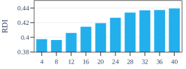
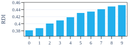
(a) $n_{\mathrm{size}}$		(b) $p_{\mathrm{cro}}\times 10^{3}$
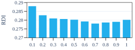
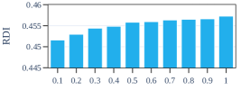
(c) $\zeta$ (five MOPS instances)		(d) $\zeta$ (twenty five LOPS instances)

Figure 10: DE performance for different parameters’ settings.

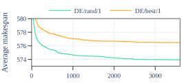
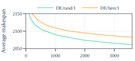
(a) five MOPS instances		(b) twenty five LOPS instances

Figure 11: Evolution of the average makespan as a function of time obtained with DE (a) with $n_{\mathrm{size}}=8$, $p_{\mathrm{cro}}=0$, and $\zeta=0.7$ applied to the five selected instances from the MOPS set and (b) with $n_{\mathrm{size}}=8$, $p_{\mathrm{cro}}=0$, and $\zeta=0.1$ applied to the twenty five selected instances from the LOPS set.

7.2.2 Genetic Algorithm

In GA there are two parameters to be calibrated, namely, $n_{\mathrm{size}}$ and $p_{\mathrm{mut}}$. Preliminary experiments indicated that varying these parameters within the ranges $n_{\mathrm{size}}\in[4,40]$ and $p_{\mathrm{mut}}\in[0.01,0.5]$ would provide acceptable results. In a first experiment, we varied $n_{\mathrm{size}}\in\{4,8,\dots,40\}$ with $p_{\mathrm{mut}}=0.25$. Figure 12a shows that the best performance is obtained with $n_{\mathrm{size}}=8$. In a second experiment, we fixed $n_{\mathrm{size}}=8$ and varied $p_{\mathrm{mut}}\in\{0.01,0.06,\dots,0.46\}$. Figures 12b and 12c show that the best performance is obtained with $p_{\mathrm{mut}}=0.36$ when the method is applied to the five selected instances from the MOPS set; while its best performance is obtained with $p_{\mathrm{mut}}=0.11$ when applied to the twenty five selected instances from the LOPS set. It can be observed that, as is happened with DE, the best population size is $n_{\mathrm{size}}=8$ and it does not depend on the size of the instances. On the other hand, the same behavior is not observed for the mutation probability parameter $p_{\mathrm{mut}}$. Similar to the parameter $\zeta$ of DE that appears in its mutation scheme, a different behavior is observed when the method is applied to instances from the MOPS and the LOPS sets. At this point, it is important to stress that this should not be considered problematic. The goal of the present work is to develop an efficient and effective method to be applied to practical instances of the OPS scheduling problem, i.e., to a real-world problem; and these instances are very similar to the instances in the LOPS set. Numerical experimentation with the MOPS instances is carried out for assessment purposes, comparing the obtained results with the ones presented in Lunardi et al. (2020a), which include numerical experiments with instances of the MOPS set.

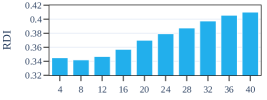
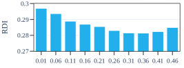
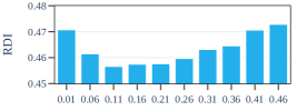
(a) $n_{\mathrm{size}}$	(b) $p_{\mathrm{mut}}$ (five MOPS instances)	(c) $p_{\mathrm{mut}}$ (twenty five LOPS instances)

Figure 12: Genetic Algorithm performance for different parameters’ settings.

7.2.3 Iterated Local Search and Tabu Search

ILS and TS have a single parameter to calibrate, namely $\hat{p}$ and $\lambda$, respectively. Preliminary experiments indicated that varying these parameters within the ranges $\hat{p}\in[1,10]$ and $\lambda\in[0.6,1.5]$ would provide acceptable results. Figures 13(a-b) show the results varying $\hat{p}\in\{1,2,\dots,10\}$ and $\lambda\in\{0.6,0.7,\dots,1.5\}$, respectively. They show that ILS performed best with $\hat{p}=2$; while TS obtained the best results with $\lambda=1.2$. It is worth noticing that, in both cases, the performance varies smoothly as a function of the parameters; thus similar performances are obtained for small variations of the parameters.

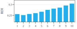
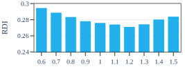
(a)	(b)

Figure 13: Performances of (a) Iterated Local Search and (b) Tabu Search as a function of their parameters $\hat{p}$ and $\lambda$.

7.3 Experiments with OPS instances

This section presents numerical experiments with the four calibrated metaheuristics DE, GA, ILS, and TS. In addition, the performance of the IBM ILOG CP Optimizer (CPO) (Laborie et al., 2018), version 12.9, is presented. CPO is a “half-heuristic-half-exact” solver specially designed to tackle scheduling problems. It has its own constraint programming (CP) modeling language to fully explore the structure of the underlying problem. In the experiments, the two-phase strategy “Incomplete model + CP Model 4” described in Lunardi et al. (2020a) is considered. This approach consists in first solving a simplified model and, in a second phase, using the solution obtained in the first phase as the initial solution to the full and more complex model. This is the approach that performed best among several alternative CP models and solution strategies considered in Lunardi et al. (2020a).

Numerical experiments consider the 20 instances in the MOPS set and the 100 instances in the LOPS set. Each metaheuristic was run 50 times in each instance of the MOPS set and 12 in each instance of the LOPS set. As described in Section 7.2, the average over all runs is considered for comparison purposes. For each run, a CPU time limit of 2 hours was imposed. The metaheuristics being evaluated start from a feasible solution and generate a sequence of feasible solutions. Thus, it is possible to observe the evolution of the makespan over time. This is not the case of the strategy of the CPO being considered. In the two-phase strategy, 2/3 of the time budget is allocated to the solution of a relaxed or incomplete OPS formulation in which setup operations can be preempted and the setup of the first operation to be processed in each machine is considered to be null; while the remaining 1/3 of the time budget is allocated to the solution of the actual CP formulation of the OPS scheduling problem. Due to the two-phase strategy, it is not possible to track the evolution of the makespan over time, since in the first 2/3 of the time budget the incumbent solution is, with high probability, infeasible. Therefore, to compare the performance of the proposed methods against the CPO, CPO was run several times with increasing time budgets given by 5 minutes, 30 minutes, and 2 hours per instance.

Figure 14 shows the evolution of the average makespan (over the 50 runs and over all instances) when the five methods are applied to the instances in the MOPS set. Table 3 presents the best makespan (in the top half of the table) and the average makespan (in the bottom half of the table) obtained by each metaheuristic method in each instance. The last line in each half of the table presents the average results. (Average of the best results in the first half and average of the average results in the second half.) In the second-half of the table, in which average results are being presented, an additional line exhibits the pooled standard deviation. For each instance, figures in bold represent the best result obtained by the methods under consideration. Average makespans and pooled standard deviations are graphically represented in Figure 15. Method TS+DE that appears in the figures and the table should be ignored at this time. The motivation for its definition as well as its presence in the experiments will be elucidated later in the current section. Table 4 shows the results of applying CPO to instances in the MOPS set. In the table, “UB” corresponds to the best solution found (upper bound to the optimal solution); while “LB” corresponds to the computed lower bound when the CPU time limit is equal to two hours. A comparison between the lower and the upper bound shows that the optimal solution was found for instances 1–5, 7, 9, 10, 13, and 15–19; while a non-null gap is reported for instances 6, 8, 11, 12, 14, and 20.

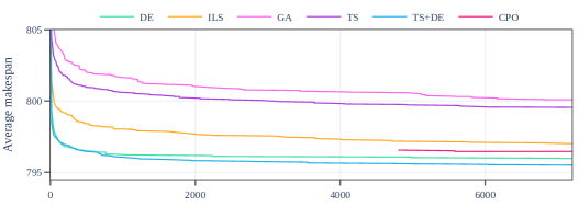
Figure 14: Evolution of the average makespan over time of each proposed method and CPO applied to the MOPS set instances.

Table 3: Results of applying the metaheuristic approaches to instances in the MOPS set.

	Best makespan
	CPU time limit: 5 minutes					CPU time limit: 30 minutes					CPU time limit: 2 hours
DE	GA	ILS	TS	TS+DE	DE	GA	ILS	TS	TS+DE	DE	GA	ILS	TS	TS+DE
1	344	351	346	344	344	344	350	346	344	344	344	350	346	344	344
2	357	358	358	357	357	357	358	357	357	357	357	357	357	357	357
3	405	409	407	409	405	405	409	407	409	404	405	409	405	408	404
4	458	458	458	458	458	458	458	458	458	458	458	458	458	458	458
5	507	516	510	507	507	507	516	510	507	507	507	516	509	507	507
6	435	447	436	437	432	435	446	436	434	432	435	442	436	433	432
7	2429	2429	2429	2429	2429	2429	2429	2429	2429	2429	2429	2429	2429	2429	2429
8	447	459	453	461	448	446	451	453	456	447	445	451	451	456	447
9	629	632	630	633	629	629	631	630	631	629	629	631	629	630	629
10	1184	1184	1184	1184	1184	1184	1184	1184	1184	1184	1184	1184	1184	1184	1184
11	413	427	419	433	414	413	426	414	433	413	413	423	414	430	413
12	491	500	496	511	492	489	492	492	511	489	489	492	492	507	489
13	347	347	347	347	347	347	347	347	347	347	347	347	347	347	347
14	392	404	396	412	389	391	404	393	408	389	389	400	391	408	389
15	320	320	319	319	319	320	319	319	319	319	320	319	319	319	319
16	543	543	543	543	543	543	543	543	543	543	543	543	543	543	543
17	1052	1052	1052	1052	1052	1052	1052	1052	1052	1052	1052	1052	1052	1052	1052
18	3184	3184	3184	3184	3184	3184	3184	3184	3184	3184	3184	3184	3184	3184	3184
19	1451	1451	1451	1451	1451	1451	1451	1451	1451	1451	1451	1451	1451	1451	1451
20	507	519	521	538	511	507	518	514	534	507	507	514	514	534	507
	794.75	799.5	796.95	800.45	794.75	794.55	798.4	795.95	799.55	794.25	794.4	797.6	795.55	799.05	794.25
	Average makespan
1	346.25	361.2	349.2	344	344.12	346	361	348	344	344.12	346	360.8	347.6	344	344.12
2	357.75	361.6	361.2	357.25	357.88	357.75	360.8	359.2	357	357.88	357.75	359	357.4	357	357.88
3	408.25	417.4	408.4	409.5	407.62	407	416	408.4	409	406.5	406.25	414.8	407.6	408.25	406.12
4	458	461.6	458	458	458	458	460	458	458	458	458	459	458	458	458
5	511	521.2	511.8	510	509.12	509.5	518.6	511.6	508	508.5	508	518.6	510.2	508	508.5
6	436.5	457.2	441.6	438	436.12	436.25	449	441	435.5	435.62	436.25	447.8	441	433.75	435.62
7	2429	2429	2429	2429	2429	2429	2429	2429	2429	2429	2429	2429	2429	2429	2429
8	451.25	463	459.2	462	452.5	450.5	461	456.2	458.75	451.12	450	460.6	453.6	456.5	450.62
9	630.5	638	630.8	637	630.5	630	632.6	630	633.5	629.88	629.75	631.8	629.6	632.25	629.5
10	1184	1184	1184	1184	1184	1184	1184	1184	1184	1184	1184	1184	1184	1184	1184
11	421.5	428.4	421.6	434.25	419.62	420	426.2	416.8	433.5	416.5	420	423.6	416.6	430.75	416
12	495	504.2	501.2	512	496.75	494.75	497.6	497.8	511.25	493.5	494	494.6	495.8	508.5	493
13	347	347	347	347	347	347	347	347	347	347	347	347	347	347	347
14	396.5	408.2	401.4	414.25	395.5	394.25	404.4	397.6	410.5	393.88	394	400.8	394.8	409	393.12
15	320	320	319.6	319	319.5	320	319.6	319	319	319.5	320	319.2	319	319	319.5
16	543	543	543	543	543	543	543	543	543	543	543	543	543	543	543
17	1052	1052	1052	1052	1052	1052	1052	1052	1052	1052	1052	1052	1052	1052	1052
18	3184	3184	3184	3184	3184	3184	3184	3184	3184	3184	3184	3184	3184	3184	3184
19	1451	1451	1451	1451	1451	1451	1451	1451	1451	1451	1451	1451	1451	1451	1451
20	511.75	523	521.4	540.25	516.75	509.25	520.8	519	536.75	512	509.25	518.2	515.4	536	507.88
Avg. 1–20	796.71	802.75	798.77	801.27	796.7	796.16	800.88	797.63	800.24	795.85	795.96	799.94	796.83	799.55	795.49
Pooled SD	1.35	5.10	2.77	1.12	1.31	1.09	4.11	2.56	0.92	1.34	1.00	3.88	2.41	0.87	1.13

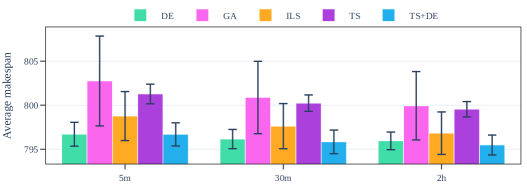
Figure 15: Average makespans and pooled standard deviations that result from applying the proposed metaheuristic approaches fifty times to instances in the MOPS set with CPU time limits of 5 minutes, 30 minutes, and 2 hours.

Table 4: Results of applying CPO to instances in the MOPS set.

Inst.	5 min.	30 min.	2 hours		Inst.	5 min.	30 min.	2 hours		Inst.	5 min.	30 min.	2 hours		Inst.	5 min.	30 min.	2 hours
	UB	UB	LB	UB		UB	UB	LB	UB		UB	UB	LB	UB		UB	UB	LB	UB
1	344	344	344	344	6	441	441	335	441	11	418	418	406	418	16	543	543	543	543
2	357	357	357	357	7	2429	2429	2429	2429	12	506	497	457	499	17	1080	1052	1052	1052
3	404	404	404	404	8	456	450	360	450	13	347	347	347	347	18	3184	3184	3184	3184
4	458	458	458	458	9	632	629	629	629	14	402	402	320	394	19	1451	1451	1451	1451
5	506	506	506	506	10	1184	1184	1184	1184	15	319	319	319	319	20	522	522	417	520
															Avg. 1–20	799.1	796.9		796.5

The results presented in Figure 14 show that DE outperforms any other method at any instant in time if the average makespan is considered. Recalling that CPO does not produce feasible solutions in the first 2/3 of the time budget, the comparison of DE with CPO requires the analysis of the results in Tables 3 and 4. The results in the tables show that DE outperforms CPO when the CPU time limit is 5 minutes, 30 minutes, or 2 hours. Results in the tables show that DE outperforms CPO also when the performance measure is the best makespan instead of the average makespan. The method that ranks in second place depends on the time limit and the performance measure (average or best makespan). Depending on the choice, CPO or ILS achieve second best result. The second place belongs to CPO when the average makespan is considered or when the CPU time limit is 2 hours. If the performance measure is the best makespan and the CPU time limit is 5 minutes or 30 minutes, the second place belongs to ILS. Concerning the best makespan and considering a CPU time limit of 2 hours, DE, GA, ILS, TS, and CPO obtained the best makespan 17, 10, 12, 12, and 13 times, respectively. Note that these numbers are slightly influenced by the presence of the method TS+DE that should be ignored. This is because TS+DE was the only method to find the best makespan in instance 6; so this instance is not computed for TS, that was the only method that found the second-best makespan for this instance. In any case, considering the average makespan, it is worth noting that, depending on whether the CPU time limit is 5 minutes, 30 minutes, or 2 hours, the difference between the methods that rank in first and last places is not larger than 0.8%, 0.7%, or 0.6%, respectively.

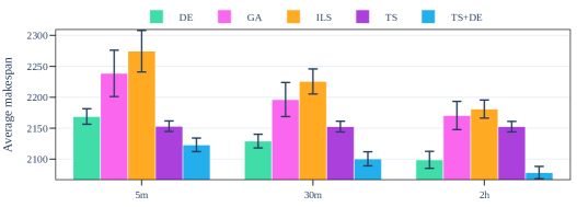
Figure 17: Average makespans and pooled standard deviations that result from applying the proposed metaheuristic approaches twelve times to instances in the LOPS set with CPU time limits of 5 minutes, 30 minutes, and 2 hours.

Figure 16 shows the evolution of the average makespan (over the 12 runs and over all instances) when the five methods are applied to the instances in the LOPS set. Tables 5 and 6 present the best makespan while Tables 7 and 8 present the average makespan obtained by each metaheuristic method in each instance when the CPU time limit is 5 minutes, 30 minutes, or 2 hours. For each instance, numbers in bold represent the best results obtained by the methods under consideration. Method TS+DE should still be ignored. At the end of Tables 5–8, “Avg. 1–50” and “Avg. 51–100” correspond to the average of the instances contained in the table; while in Tables 6 and 8, “Avg. 1–100” corresponds to the average over the whole LOPS set. In Table 8, and additional line exhibits the pooled standard deviation. Average makespans and pooled standard deviations are graphically represented in Figure 17. Table 9 shows the results of applying CPO to the instances in the LOPS set. The symbol “ — ” means that CPO was not able to find a feasible solution within the time budget.

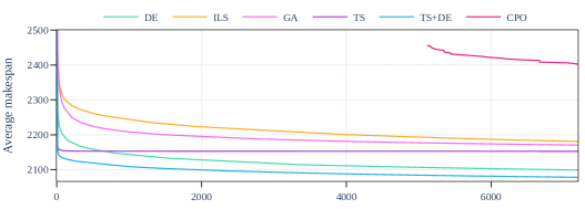
Figure 16: Evolution of the average makespan over time of each proposed method and CPO applied to the LOPS set instances.

Table 5: Best makespan that results from applying the metaheuristics to the first-half of the instances in the LOPS set.

Instance	CPU time limit: 5 minutes					CPU time limit: 30 minutes					CPU time limit: 2 hours
	DE	GA	ILS	TS	TS+DE	DE	GA	ILS	TS	TS+DE	DE	GA	ILS	TS	TS+DE
1	516	525	516	527	516	516	522	516	526	516	513	520	516	524	514
2	641	655	647	660	642	641	651	647	659	641	638	648	642	658	639
3	620	623	622	644	617	615	622	616	644	614	613	618	612	640	613
4	741	750	736	769	742	736	743	736	767	738	736	741	736	767	737
5	826	836	829	857	824	820	831	821	856	821	820	824	820	854	820
6	689	691	690	726	683	681	683	679	724	678	676	679	674	724	675
7	896	903	896	935	897	890	895	892	935	888	886	894	890	935	886
8	1007	1014	1013	1049	1010	1001	1005	1004	1049	1000	999	1002	999	1049	997
9	919	921	920	969	915	905	914	911	969	906	902	910	906	969	900
10	765	775	768	829	762	748	764	754	829	752	745	755	749	829	744
11	1182	1191	1182	1217	1174	1165	1183	1167	1217	1162	1160	1164	1161	1217	1153
12	1168	1183	1170	1227	1164	1146	1162	1150	1227	1149	1138	1155	1138	1227	1140
13	988	1001	994	1055	990	971	986	976	1055	974	961	980	965	1055	965
14	1443	1450	1443	1498	1436	1430	1443	1428	1498	1427	1421	1431	1419	1498	1419
15	1386	1398	1384	1454	1380	1366	1384	1360	1454	1362	1355	1373	1356	1454	1352
16	1311	1327	1306	1366	1312	1293	1308	1288	1366	1293	1284	1301	1280	1366	1282
17	1041	1061	1041	1085	1045	1028	1046	1030	1085	1029	1019	1030	1016	1085	1021
18	1885	1898	1880	1956	1885	1862	1875	1855	1956	1859	1848	1858	1840	1956	1843
19	990	1007	997	1025	989	978	992	980	1025	974	962	985	964	1025	968
20	965	988	971	1013	967	948	969	952	1013	949	932	955	934	1013	934
21	1879	1894	1881	1948	1878	1852	1866	1853	1948	1854	1837	1850	1834	1948	1835
22	1417	1424	1442	1477	1402	1380	1404	1406	1477	1359	1361	1381	1383	1477	1349
23	1070	1083	1074	1105	1074	1050	1062	1056	1105	1059	1038	1050	1037	1105	1040
24	1914	1935	1921	1974	1919	1884	1905	1894	1974	1882	1859	1887	1870	1974	1857
25	1227	1245	1238	1272	1222	1204	1223	1209	1272	1205	1189	1208	1194	1272	1191
26	1281	1306	1293	1309	1279	1256	1284	1259	1309	1261	1237	1264	1238	1309	1243
27	1698	1718	1715	1753	1696	1670	1683	1677	1753	1670	1652	1674	1651	1753	1648
28	1929	1944	1953	1988	1926	1885	1925	1901	1988	1877	1858	1892	1879	1988	1853
29	2011	2072	2097	2098	1977	1950	2017	2009	2098	1943	1909	1986	1958	2098	1905
30	1557	1571	1576	1586	1548	1521	1546	1535	1586	1516	1496	1527	1510	1586	1487
31	1164	1185	1221	1179	1133	1128	1155	1167	1179	1103	1100	1136	1127	1179	1089
32	1062	1079	1094	1086	1058	1050	1062	1057	1086	1043	1034	1053	1039	1086	1030
33	2095	2114	2145	2151	2092	2058	2094	2086	2151	2052	2033	2075	2053	2151	2025
34	1438	1429	1465	1437	1390	1391	1405	1419	1437	1361	1356	1390	1388	1437	1342
35	2772	2835	2877	2895	2795	2732	2789	2795	2895	2740	2689	2754	2726	2895	2694
36	2482	2504	2549	2544	2478	2446	2482	2492	2544	2445	2419	2463	2443	2544	2417
37	1275	1299	1307	1287	1271	1253	1278	1281	1287	1247	1236	1263	1263	1287	1238
38	1159	1164	1182	1169	1145	1145	1142	1154	1169	1135	1125	1134	1133	1169	1119
39	1756	1754	1787	1760	1733	1721	1739	1758	1760	1706	1692	1714	1728	1760	1688
40	2204	2220	2261	2226	2181	2174	2200	2213	2226	2154	2142	2186	2163	2226	2131
41	2316	2344	2345	2304	2251	2268	2307	2281	2304	2229	2231	2275	2246	2304	2194
42	1582	1605	1655	1559	1539	1546	1565	1591	1559	1521	1520	1551	1551	1559	1502
43	2523	2540	2574	2548	2507	2490	2535	2526	2548	2486	2457	2500	2496	2548	2449
44	3678	3776	3839	3695	3638	3645	3715	3771	3695	3571	3578	3663	3702	3695	3516
45	2060	2065	2143	2069	2051	2043	2054	2095	2069	2033	2021	2044	2055	2069	2014
46	2185	2199	2236	2220	2180	2153	2185	2187	2220	2150	2122	2163	2150	2220	2123
47	3413	3539	3689	3438	3363	3356	3491	3602	3438	3330	3297	3454	3515	3438	3273
48	1272	1287	1313	1260	1242	1250	1274	1276	1260	1231	1231	1255	1256	1260	1218
49	2862	2893	2933	2889	2851	2836	2876	2886	2889	2829	2816	2844	2844	2889	2804
50	1374	1382	1403	1369	1347	1349	1369	1380	1369	1333	1331	1356	1359	1369	1321
Avg. 1–50	1532.7	1552.0	1564.3	1569.1	1522.3	1508.5	1532.2	1531.6	1569.0	1501.1	1489.5	1516.3	1508.2	1568.8	1483.9

Table 6: Best makespan that results from applying the metaheuristics to the second-half of the instances in the LOPS set.

Instance	CPU time limit: 5 minutes					CPU time limit: 30 minutes					CPU time limit: 2 hours
	DE	GA	ILS	TS	TS+DE	DE	GA	ILS	TS	TS+DE	DE	GA	ILS	TS	TS+DE
51	1567	1590	1649	1595	1557	1549	1573	1608	1595	1543	1530	1554	1573	1595	1527
52	1956	2034	2099	1952	1913	1920	1984	2040	1952	1888	1886	1952	1985	1952	1868
53	3629	3639	3678	3668	3623	3590	3614	3643	3668	3588	3555	3585	3599	3668	3549
54	1553	1578	1596	1542	1535	1535	1554	1563	1542	1525	1526	1542	1545	1542	1514
55	2001	2021	2082	1998	1986	1975	1999	2036	1998	1970	1953	1984	1993	1998	1944
56	2582	2584	2635	2577	2554	2552	2562	2602	2577	2535	2528	2537	2567	2577	2509
57	1917	1947	1989	1892	1878	1888	1936	1960	1892	1865	1873	1892	1907	1892	1857
58	1814	1841	1890	1807	1779	1790	1822	1853	1807	1764	1769	1795	1802	1807	1739
59	3415	3440	3485	3432	3411	3393	3418	3448	3432	3388	3356	3394	3408	3432	3355
60	1994	2044	2056	2004	1981	1970	2015	2031	2004	1966	1948	1998	2001	2004	1945
61	1988	2049	2127	2014	1980	1950	2034	2078	2014	1953	1930	2003	2032	2014	1934
62	3224	3289	3346	3138	3113	3137	3238	3284	3138	3108	3107	3200	3226	3138	3075
63	2512	2623	2727	2522	2495	2451	2574	2657	2522	2448	2412	2561	2571	2522	2416
64	1875	1933	1973	1911	1866	1858	1914	1948	1911	1857	1842	1897	1915	1911	1844
65	1909	1964	2047	1935	1893	1880	1951	2030	1935	1874	1860	1939	1994	1935	1852
66	1773	1813	1892	1761	1748	1750	1802	1878	1761	1747	1743	1794	1837	1761	1734
67	1687	1734	1755	1678	1671	1670	1714	1741	1678	1666	1658	1682	1712	1678	1653
68	3259	3385	3472	3074	3023	3081	3315	3425	3068	2967	2967	3272	3337	3068	2922
69	3037	3406	3479	2921	2891	2902	3296	3346	2921	2863	2844	3223	3220	2921	2831
70	3240	3269	3508	3161	3123	3121	3248	3461	3161	3053	2997	3227	3376	3161	2973
71	2179	2247	2280	2189	2173	2167	2228	2252	2189	2158	2145	2217	2227	2189	2142
72	1957	2031	2073	1802	1790	1880	1986	2024	1802	1787	1802	1964	1961	1802	1763
73	3967	3992	4086	3940	3915	3907	3981	4062	3940	3902	3867	3964	4013	3940	3869
74	4342	4355	4389	4260	4238	4228	4341	4354	4260	4199	4171	4290	4313	4260	4157
75	3635	3667	3712	3655	3632	3607	3642	3684	3655	3612	3583	3629	3653	3655	3585
76	2444	2570	2638	2264	2266	2362	2519	2585	2252	2221	2250	2481	2522	2252	2184
77	1799	1864	1904	1792	1777	1770	1846	1879	1792	1764	1751	1829	1837	1792	1750
78	1671	1694	1748	1669	1659	1650	1685	1716	1669	1650	1634	1671	1686	1669	1634
79	1750	1799	1841	1751	1738	1736	1786	1803	1751	1733	1726	1759	1777	1751	1722
80	1788	1891	1893	1739	1732	1745	1832	1864	1739	1723	1711	1804	1819	1739	1697
81	3253	3260	3375	3145	3140	3171	3189	3354	3145	3122	3140	3171	3327	3145	3086
82	4691	4742	4784	4693	4683	4665	4706	4757	4693	4659	4635	4687	4732	4693	4634
83	3122	3175	3192	3125	3091	3088	3160	3174	3125	3072	3062	3136	3144	3125	3050
84	2020	2056	2121	1960	1951	1961	2026	2076	1960	1942	1940	2008	2042	1960	1931
85	2400	3132	3196	2379	2367	2369	2919	2972	2379	2344	2344	2819	2756	2379	2332
86	2330	2786	2966	2296	2267	2282	2507	2760	2296	2248	2246	2425	2521	2296	2237
87	3230	3315	3455	2962	2938	3137	3243	3390	2962	2909	3055	3203	3311	2962	2876
88	5401	5481	5523	5405	5382	5358	5399	5490	5405	5351	5316	5372	5455	5405	5315
89	3863	3943	3942	3760	3737	3760	3858	3893	3760	3720	3716	3844	3864	3760	3681
90	3350	3438	3491	3328	3310	3344	3389	3476	3328	3280	3308	3380	3439	3328	3257
91	2456	2598	2637	2418	2401	2421	2523	2585	2418	2376	2380	2506	2550	2418	2357
92	3579	3659	3724	3212	3248	3540	3622	3662	3167	3212	3423	3560	3610	3167	3205
93	2194	2260	2372	2144	2127	2155	2213	2311	2144	2116	2137	2201	2263	2144	2111
94	4458	4543	4616	4430	4407	4422	4503	4581	4430	4393	4378	4471	4557	4430	4370
95	2647	2763	2827	2607	2580	2601	2675	2767	2607	2570	2571	2648	2746	2607	2548
96	3437	3588	3622	3112	3120	3384	3533	3600	3112	3087	3296	3505	3559	3112	3046
97	2538	2837	3204	2547	2518	2517	2708	2981	2547	2506	2491	2646	2763	2547	2487
98	5566	5637	5692	5534	5511	5506	5601	5664	5534	5484	5458	5562	5632	5534	5455
99	2146	2236	2227	1972	1989	2105	2192	2196	1972	1983	2065	2169	2179	1972	1969
100	3340	3399	3426	3306	3294	3310	3356	3397	3306	3291	3270	3343	3384	3306	3265
Avg. 51–100	2769.7	2862.8	2928.8	2719.6	2700.0	2722.2	2814.6	2878.8	2718.3	2679.6	2683.1	2785.9	2824.8	2718.3	2655.1
Avg. 1–100	2151.2	2207.4	2246.6	2144.4	2111.2	2115.4	2173.4	2205.2	2143.7	2090.4	2086.3	2151.1	2166.5	2143.6	2069.5

Table 7: Average makespan that results from applying the metaheuristics to the first-half of the instances in the LOPS set.

Instance	CPU time limit: 5 minutes					CPU time limit: 30 minutes					CPU time limit: 2 hours
	DE	GA	ILS	TS	TS+DE	DE	GA	ILS	TS	TS+DE	DE	GA	ILS	TS	TS+DE
1	519	528.5	520.5	528.5	521	517	524.2	518.8	526.5	518.9	515.8	523.8	518.5	524.8	518.1
2	650	657.2	650.8	661.5	647.6	647.5	653	648	659.5	644	644.2	651.5	644.2	659.2	641.4
3	621	625.8	623.5	647.5	621.2	618	622.8	621.5	645.5	617.6	616.5	620.8	618.5	642.8	615.4
4	743.8	752.2	745.5	771.2	745.6	738	745	741	769.2	741.6	737.5	743	739.8	768.5	739.2
5	827.8	839.5	833.5	861.5	828.2	824.5	832	827.8	857.2	824.6	821.2	828.5	822.8	856.5	822
6	692.8	702.8	695.5	728.8	690.5	683	690	685	726.5	681.4	676.8	685.8	679.5	724.8	677.6
7	897.2	910.8	902	942	898.4	893.2	899.8	895	940.5	892.4	889.5	896	892.8	939.2	888.8
8	1012	1020.2	1019	1052	1013.5	1004.8	1008.5	1006.5	1052	1005	999.8	1005.2	1003.2	1052	1000.8
9	922	935	925.2	977.8	921.8	911.2	925.2	912.2	977.8	910.2	905.2	912.5	907.8	977.8	904.9
10	766.8	785.5	773.8	831.5	768.6	751.8	768.2	761	831.5	754.9	746.8	760.5	750.5	831.2	748.6
11	1188.2	1201.8	1190.2	1227.5	1179.1	1174.5	1185.5	1171.8	1227.5	1166.4	1163.2	1174.8	1162.5	1227.5	1158.4
12	1172	1191.8	1184	1229	1170.9	1156.8	1177.5	1153.8	1228.2	1154.4	1146.8	1164.8	1141.5	1228.2	1145
13	997.5	1006.5	1004.8	1064.5	997	976	994	983	1064.5	980.9	967	983	970.8	1064.5	968.4
14	1446.5	1458.8	1447.5	1504.5	1447.4	1433.5	1449.2	1433.8	1504.5	1432.6	1426.2	1436.2	1423.8	1504.5	1424.8
15	1394.8	1407.8	1394.8	1468.2	1386.9	1370.5	1390.2	1369	1466.2	1367.6	1358.5	1376	1359.5	1465.2	1355.2
16	1317.5	1331.5	1320.5	1371	1315.8	1296.8	1314	1301.2	1371	1297	1286.8	1305	1286.8	1371	1287.4
17	1047	1067.8	1047	1087.5	1049.5	1032.8	1047.2	1034.5	1087.5	1033.8	1024	1032.5	1020	1087.5	1024.2
18	1889.2	1901	1886	1966.2	1892.4	1866.2	1878.8	1863	1966.2	1863.4	1855.2	1863.2	1844.8	1966.2	1850.4
19	995.2	1010.2	1000.8	1028.2	994.2	981.5	995.8	984.5	1028.2	980.6	970.8	988	970.8	1028.2	970.6
20	977.5	990.5	977.8	1019.5	977.6	955.8	980.5	954.8	1019.5	956.8	941.8	964.8	935.2	1019.5	939.6
21	1889.2	1911.8	1894.5	1957	1888.8	1859	1874.5	1860.2	1957	1858.6	1845.8	1859.8	1841.5	1957	1841.8
22	1421.5	1435.5	1469.2	1487.2	1408	1385.2	1410.2	1414	1487.2	1375.6	1364	1393	1392.8	1487.2	1357.9
23	1076.8	1090	1087	1109.5	1081.8	1055.5	1076.8	1067	1109.5	1062.1	1043	1061.5	1046.2	1109.5	1048.5
24	1923.8	1946	1938.5	1978	1922.9	1889.5	1918	1906	1978	1886.4	1870.8	1902	1879.2	1978	1866.2
25	1232.5	1254.2	1244.8	1281	1228.8	1208.5	1229.8	1215.5	1281	1208	1193.5	1212.5	1199.5	1281	1194.1
26	1286.8	1310.2	1307.8	1326.2	1287.6	1263.8	1292.5	1271.2	1326.2	1270.2	1242	1279.2	1244	1326.2	1249.2
27	1704.5	1727.8	1732.8	1761.8	1705.1	1676	1707.5	1690.8	1761.8	1675.6	1653	1686.2	1663.8	1761.8	1654.9
28	1935.2	1956.2	1993	1999.2	1931.9	1898.2	1931	1931.5	1999.2	1884.6	1872.5	1899.2	1894	1999.2	1861.8
29	2019.5	2075.8	2113.2	2108.2	1999.8	1968.8	2032.5	2029.5	2108.2	1953.2	1930.2	1989.5	1983	2108.2	1918.4
30	1565	1573.2	1588.5	1595.8	1557.5	1529.2	1551.2	1550.5	1595.8	1521.5	1503.5	1534	1516	1595.8	1496.8
31	1170	1207	1231.8	1182.8	1141.5	1131	1176	1178.2	1182.8	1111.4	1105.5	1151.5	1137	1182.8	1092.2
32	1074.2	1084	1102.8	1091	1061.4	1054.2	1067.5	1066.5	1091	1046.2	1039.2	1056.8	1044.5	1091	1034
33	2100.2	2123	2161.2	2164	2099.1	2068.8	2101.5	2096	2164	2064.2	2036.2	2087	2062.5	2164	2034.5
34	1454.5	1451.5	1493.8	1443.5	1404.4	1406.5	1427	1435.5	1443.5	1368.9	1369.2	1399	1401	1443.5	1345.2
35	2818.8	2867	2922	2907.2	2816	2744.8	2817.5	2827.8	2907.2	2748.5	2700.5	2786.8	2752.8	2907.2	2705.8
36	2494.8	2522.2	2604.8	2548.8	2483.1	2456.5	2486.8	2524.2	2548.8	2451	2425	2468.8	2467	2548.8	2420.1
37	1281.8	1304.5	1316.2	1290.8	1274.4	1263.2	1287.5	1290.2	1290.8	1256.1	1241.2	1270.2	1267	1290.8	1241.1
38	1173.5	1177.8	1192.8	1173.8	1150.4	1151.8	1156	1159.8	1173.8	1137.1	1131.5	1143.8	1137.2	1173.8	1122.8
39	1768.5	1794.2	1800	1767	1739.1	1734.8	1762	1764	1767	1716	1706	1738.8	1736.8	1767	1693.4
40	2217.2	2235.2	2289.5	2236.2	2189.6	2180.8	2210.5	2234.2	2236.2	2162.9	2148.8	2192.8	2184.2	2236.2	2135.9
41	2332	2386.5	2355.8	2323	2278.5	2278.5	2342.5	2294.8	2323	2247.8	2243	2296.8	2261.2	2323	2209.9
42	1601.2	1618	1668.2	1570.2	1542.9	1559	1585.2	1602.2	1570.2	1527.6	1530	1561.8	1558.2	1570.2	1506.1
43	2530.8	2567.5	2601.8	2552	2522.4	2498.8	2545.5	2557.8	2552	2491.1	2460.2	2529.2	2515.2	2552	2458.6
44	3748	3835.2	3886.8	3716	3673.6	3680.8	3774.5	3812.5	3716	3614.1	3629.5	3746.8	3744.8	3716	3545
45	2082.5	2116	2151.8	2077	2054.1	2053.2	2086.8	2100.5	2077	2038	2028	2065.8	2059.2	2077	2020
46	2190.2	2215	2258	2225.5	2186	2160.2	2192	2198.8	2225.5	2155.6	2133.8	2168.8	2154.8	2225.5	2128.6
47	3434.5	3753.5	3822.2	3461.8	3389.8	3369	3671.5	3720.2	3461.8	3336.8	3313	3586.2	3618.5	3461.8	3285.6
48	1280.8	1293.8	1342.5	1263.2	1247.9	1259	1285	1296	1263.2	1236.1	1236	1264	1264.8	1263.2	1222.9
49	2885.5	2927	2947.2	2896.8	2864.5	2847.8	2898.5	2895.2	2896.8	2838.6	2822.8	2866.2	2853.5	2896.8	2811.4
50	1378.5	1389.8	1417.5	1377.8	1353.8	1354.2	1373.5	1394.8	1377.8	1339	1335	1360	1366.8	1377.8	1326.1
Avg. 1–50	1543.0	1569.5	1581.6	1576.8	1531.0	1516.4	1547.1	1545.0	1576.4	1508.1	1496.9	1529.5	1518.8	1576.2	1490.2

Table 8: Average makespan that results from applying the metaheuristics to the second-half of the instances in the LOPS set.

Instance	CPU time limit: 5 minutes					CPU time limit: 30 minutes					CPU time limit: 2 hours
	DE	GA	ILS	TS	TS+DE	DE	GA	ILS	TS	TS+DE	DE	GA	ILS	TS	TS+DE
51	1585.8	1611.5	1668.5	1598.2	1564.5	1561	1591.2	1621.8	1598.2	1546.8	1539.5	1571	1584.5	1598.2	1530.9
52	1979	2060.2	2159	1964	1920.4	1933.8	2007.5	2078	1964	1895.2	1896.5	1971	2001.8	1964	1873.9
53	3637.5	3645.8	3683.5	3672	3628.6	3598.5	3618	3645	3672	3592.4	3563.2	3590	3601	3672	3556.4
54	1566	1578.8	1606	1555.5	1538.4	1546.2	1561.2	1575	1555.5	1529.9	1530.2	1547.2	1553.5	1555.5	1516.6
55	2009	2058	2096	2013	1993.1	1982.8	2022.8	2048.8	2013	1972.4	1962	1997.5	1999.5	2013	1951.2
56	2597	2610.8	2647.8	2586.8	2565.5	2563.5	2589	2612	2586.8	2542.6	2535.8	2569.2	2574.2	2586.8	2515.9
57	1955.2	1957.2	2055	1906.5	1884.6	1928.2	1948.5	1999	1906.5	1872.8	1883.5	1920.5	1925.5	1906.5	1859
58	1822.2	1847.5	1897	1812.2	1786.8	1799	1830.2	1858.5	1812.2	1773.5	1780.8	1811	1814.5	1812.2	1754.1
59	3429	3454.8	3494.2	3442.2	3416.9	3400.2	3430	3459	3442.2	3393.4	3365.2	3408	3421.8	3442.2	3363.4
60	1998.8	2050.2	2076	2006.5	1987.9	1976.2	2024	2039.8	2006.5	1970.9	1953.2	2005	2007.2	2006.5	1953.2
61	2001	2070.5	2139.2	2025.5	1989.8	1962.8	2046.5	2081.8	2025.5	1963	1932.2	2014.5	2035.2	2025.5	1937.9
62	3280.5	3350.8	3366.2	3158	3121.2	3187.8	3273.5	3311.8	3158	3111.5	3116.5	3232.5	3246.8	3158	3104.6
63	2538.5	2648.2	2742.8	2540.8	2506.1	2465.5	2605.5	2686.2	2540.8	2459.6	2424.8	2569	2596	2540.8	2422.6
64	1883.2	1952.5	2005.5	1914.8	1879.6	1863	1925	1981	1914.8	1860.5	1845.8	1903.8	1937	1914.8	1845.1
65	1945.2	1992.5	2100.2	1939.5	1906	1892.2	1976	2049.2	1939.5	1884.2	1866	1957	2003	1939.5	1862.6
66	1791.5	1850.5	1927.8	1767.2	1752.4	1755.8	1827.5	1891	1767.2	1749	1746.5	1808	1846	1767.2	1743.8
67	1698	1766.2	1794.2	1685.2	1677.2	1678.5	1728.5	1765.2	1685.2	1670.2	1662.5	1704	1727.8	1685.2	1658.4
68	3386.5	3444.8	3488.8	3082	3073.4	3234	3358	3440.2	3080	2985.2	3052.8	3324	3364.5	3080	2930.1
69	3087.5	3443.5	3522	2945.2	2904	2924	3309.5	3388.8	2945.2	2871.9	2859	3239.2	3261.8	2945.2	2835.9
70	3246.5	3342.2	3544	3178	3141.5	3158.5	3308.5	3474.8	3178	3078.6	3069.5	3274	3395.2	3178	2989.8
71	2211.5	2270.2	2315	2196.5	2181.6	2179.2	2251	2284.2	2196.5	2166.4	2151.2	2229.2	2245	2196.5	2147.5
72	1979.5	2070.5	2094.8	1815.5	1801.1	1891.8	2023	2039.5	1815.5	1793	1811.8	1987.8	1970.2	1815.5	1774.5
73	3982	4048.5	4114.8	3951.5	3925.2	3929.5	4006.2	4078.8	3951.5	3911.1	3890.2	3983	4033.8	3951.5	3879.8
74	4398	4416.2	4418.8	4286.2	4265.5	4291.5	4348.5	4373.2	4286.2	4232.4	4229.8	4306.2	4329.8	4286.2	4176.5
75	3639.5	3688.5	3717.5	3662.2	3635.5	3610.8	3663.5	3684.8	3662.2	3615.1	3588.2	3642.5	3657.5	3662.2	3589
76	2514.2	2619.2	2664	2267	2343.6	2391	2560	2597.5	2261.2	2280	2300.2	2518.5	2535.8	2261.2	2221.2
77	1806.2	1889.2	1919.2	1798.2	1781.2	1774.8	1854.2	1887.8	1798.2	1770.9	1760.2	1834.2	1843.8	1798.2	1760
78	1681.8	1724.5	1773.2	1676.2	1664	1653.8	1699.2	1734	1676.2	1654.8	1636	1685.5	1695.8	1676.2	1636.9
79	1759.8	1829	1844.5	1756.5	1745.6	1743.2	1793.8	1811.8	1756.5	1738.6	1727.5	1770.5	1781	1756.5	1726.2
80	1801.2	1900	1907.5	1746.2	1741.8	1760.2	1842	1875.2	1746.2	1731.6	1731.8	1821	1827.8	1746.2	1705.6
81	3260	3309.5	3387.8	3149.5	3144.2	3206	3243	3363	3149.5	3136.8	3150.8	3216.8	3330.2	3149.5	3107.5
82	4712.5	4761.8	4797.8	4705	4689.5	4682.2	4724.2	4773	4705	4666.6	4646.5	4703.2	4749.5	4705	4638.6
83	3141.8	3200.8	3224.5	3134.8	3102.4	3097.2	3169	3198.5	3134.8	3081.4	3063.2	3151.8	3170.2	3134.8	3056.9
84	2038	2103	2163	1961.2	1960.6	1974.5	2067.2	2108.2	1961.2	1951.9	1957.8	2041.5	2061.2	1961.2	1937.6
85	2473.8	3222	3236.2	2395.5	2375.5	2398.2	3010	3027.2	2395.5	2357.5	2359.2	2885	2791.8	2395.5	2340.2
86	2345.8	2875.8	3005.5	2310.8	2282.8	2303	2629	2774	2310.8	2265.2	2258	2530.5	2565.8	2310.8	2242.2
87	3253.8	3375.5	3535	2975.2	2990.2	3157.8	3292.5	3424.5	2975.2	2949.8	3097.8	3246.8	3330	2975.2	2908.5
88	5413	5495.2	5534.5	5415.5	5395.2	5369.8	5432.2	5504	5415.5	5362.2	5324.5	5400.2	5464.5	5415.5	5323
89	3884	3998.5	4004.8	3765.8	3748	3818	3917	3951.2	3765.8	3729.5	3762.8	3869.5	3906.5	3765.8	3693.4
90	3369.5	3504	3514.5	3334.2	3330.1	3345	3434.2	3490.8	3334.2	3310.4	3329.2	3411.8	3455.8	3334.2	3288.5
91	2501.8	2622	2823	2428.2	2408.8	2431.2	2559.2	2656.2	2428.2	2388.5	2400.8	2526	2590	2428.2	2362
92	3609	3743.2	3776	3224.5	3274.8	3559.5	3654	3719.5	3199.8	3237.4	3499.5	3603.2	3642.5	3197	3210.1
93	2202.2	2320.5	2422.8	2148	2145.8	2168.5	2261.8	2325.5	2148	2138.9	2148.5	2227.2	2269.8	2148	2133
94	4474.5	4579.2	4639.5	4441	4427.2	4433.2	4525	4597.8	4441	4409.8	4389.8	4494.8	4568.8	4441	4380
95	2702.5	2834.8	2872.5	2609.8	2594.1	2616.2	2748.2	2806.8	2609.8	2578.9	2581.8	2713	2762.2	2609.8	2558.1
96	3487.5	3658.5	3683.8	3123.2	3192.8	3418.2	3572	3628.5	3123.2	3153.1	3336.2	3529.8	3588.5	3123.2	3108.4
97	2560.8	3185.2	3427.5	2556.8	2532.2	2527.8	2776	3197	2556.8	2511.4	2496.2	2682	2813	2556.8	2490.5
98	5589	5698.8	5714.5	5548	5516.1	5524.8	5631	5682	5548	5496.2	5477.5	5584.8	5646.5	5548	5461
99	2157.2	2265.2	2322.5	1986.5	2013.8	2114.2	2204	2246	1986.5	2003.4	2071.8	2177	2194.2	1986.5	1985.8
100	3349	3434.5	3494.5	3313.5	3309	3317.8	3403.5	3454.2	3313.5	3295.6	3281.8	3388.5	3431.5	3313.5	3271.6
Avg. 51–100	2794.7	2907.6	2967.3	2729.5	2715.1	2742.0	2845.5	2906.0	2728.9	2692.8	2700.9	2811.6	2843.0	2728.8	2666.4
Avg. 1–100	2168.9	2238.6	2274.5	2153.2	2123.1	2129.2	2196.3	2225.5	2152.7	2100.5	2098.9	2170.6	2180.9	2152.5	2078.3
Pooled SD	12.43	37.38	33.54	8.59	10.93	11.13	27.58	20.18	8.61	11.33	13.71	22.70	14.53	8.58	9.97

Table 9: Results of applying CPO to the instances in the LOPS set.

Inst.	5 min.	30 min.	2 hours		Inst.	5 min.	30 min.	2 hours		Inst.	5 min.	30 min.	2 hours		Inst.	5 min.	30 min.	2 hours
	UB	UB	LB	UB		UB	UB	LB	UB		UB	UB	LB	UB		UB	UB	LB	UB
1	538	530	387	527	26	1581	1486	880	1362	51	2130	1991	521	1734	76	—	—	639	2637
2	663	654	494	650	27	1833	1791	1246	1790	52	2540	2236	553	2091	77	—	—	604	2010
3	653	635	452	633	28	2185	2171	1396	2089	53	4711	3836	523	3860	78	—	—	636	1960
4	780	755	562	756	29	2256	2298	1452	2199	54	3074	2086	533	1661	79	—	—	560	2379
5	860	837	625	828	30	2473	1590	1116	1769	55	2416	2386	497	2295	80	—	—	654	2392
6	724	718	490	715	31	1296	1295	822	1218	56	2876	2939	510	2706	81	—	—	693	3377
7	964	938	659	923	32	1214	1208	776	1151	57	2413	2683	584	2169	82	—	5339	624	5276
8	1091	1044	739	1039	33	2698	2398	1469	2276	58	2520	2045	823	1993	83	—	3346	701	3355
9	1019	966	654	980	34	1545	1604	951	1483	59	3800	3998	511	3764	84	—	—	672	2231
10	902	900	547	790	35	3145	3099	1932	3049	60	2375	2236	587	2577	85	—	—	818	3786
11	1290	1231	857	1230	36	3167	2819	1788	2826	61	—	—	582	2845	86	—	—	918	3065
12	1257	1223	838	1180	37	1463	1671	924	1468	62	3845	3352	658	3341	87	—	—	696	3388
13	1084	1010	699	1011	38	1264	1200	832	1192	63	3169	2934	1392	2782	88	—	5963	671	5956
14	1557	1514	1052	1486	39	1880	1870	1214	1845	64	2960	2123	914	2104	89	—	—	1374	4068
15	1542	1476	975	1445	40	2463	2509	1552	2439	65	—	—	584	2061	90	—	—	646	3616
16	1516	1420	924	1382	41	2550	2522	1587	2524	66	—	—	611	1924	91	—	—	728	3449
17	1131	1080	763	1117	42	1732	1688	1111	1715	67	—	—	804	1930	92	—	—	712	3769
18	2014	1918	1415	1897	43	2784	2779	1737	2767	68	3858	3343	642	3238	93	—	—	751	2392
19	1236	1046	737	1028	44	4030	4063	2587	3908	69	3787	3346	615	3518	94	—	—	780	4883
20	1135	1132	671	1053	45	2378	2466	1446	2301	70	4037	4340	629	4172	95	—	—	726	3051
21	2104	1992	1378	1956	46	2439	2497	1539	2446	71	3771	2417	598	2435	96	—	—	1555	3662
22	1639	1642	985	1496	47	4195	3757	2518	4040	72	—	—	943	1949	97	—	—	1650	3976
23	1336	1128	762	1146	48	1377	1506	896	1473	73	4946	4304	624	4376	98	—	—	716	6117
24	2135	2073	1377	2010	49	4065	3012	2108	3233	74	5062	4668	713	4602	99	—	—	690	2825
25	1524	1442	892	1367	50	2244	1570	931	1505	75	4185	4177	711	4046	100	—	—	682	3717
															Avg. 1–100	2263.4	2195.4		2402.2

The results in Figure 16 show that, differently from the previous experiments with the medium-sized OPS instances, in the large-sized instances no method obtains the smallest average makespan regardless of the considered time instant. TS outperforms all the other methods for any instant $t\leq 650$ seconds while DE outperforms all the other methods for any instant $t\geq 650$ seconds. Another difference concerning the medium-sized instances is that CPO was outperformed by all introduced metaheuristic approaches. The numerical values in Tables 5–8 reflect the results already observed in Figure 16. TS found the best results for small-time limits while DE found the best results for large time limits. From the average results at the end of Tables 6 and 8 we can see that the methods rank (a) TS, DE, GA, ILS, and CPO; (b) DE, TS, GA, ILS, and CPO; and (c) DE, TS, GA, ILS, and CPO, when the CPU time limit is 5 minutes, 30 minutes, and 2 hours, respectively, independently of whether we consider the best or the average makespan as a performance measure.

The observations described in the paragraph above led us to consider a combined approach, named TS+DE, that uses TS to construct an initial population for DE. The combined approach has three phases. In the first phase, TS is used to obtain a solution. Instead of running the method until it reaches the CPU time limit, the search is stopped if the incumbent solution is not updated during a period of $\log_{10}(o)$ seconds of CPU time, recalling that $o$ is the number of operations of an instance. In the second phase, a population is constructed by running the local search procedure starting from $n_{\mathrm{size}}-1$ perturbations of the TS solution. The perturbation procedure is the one described for the ILS algorithm in Section 6. The solution of the TS plus the $n_{\mathrm{size}}-1$ solutions found with the local search constitute the initial population of DE. Running DE with this initial population is the third phase of the strategy. The three-phase strategy is interrupted at any time if the CPU time limit is reached. In this strategy, parameters of TS, DE, and the perturbation procedure of ILS were set as already calibrated for each individual method.

Figure 14 and Table 3 show the performance of the combined approach when applied to the OPS instances in the MOPS set while Figure 16 and Tables 5–8 show the performance of the combined approach when applied to the OPS instances in the LOPS set. Specifically for the instances in the MOPS set, TS+DE (with a CPU time limit of at least 30 minutes) finds the optimal solutions in the 14 instances with the known optimal solution and improves the solutions found by CPO in the 6 instances with a non-null gap. Figures and tables show that TS+DE is the most successful approach. It always found the lowest average makespan in the MOPS and LOPS sets independent of the CPU time limit imposed. It found the lowest best and average makespans and it found the largest number of best solutions among all considered methods, outperforming CPO by a large extent. It is worth noting that, in the LOPS set, considering the average makespan, the difference between the metaheuristics that rank in first and last places is not larger than 7%, 6%, or 5%, depending on whether the CPU time limit is 5 minutes, 30 minutes, or 2 hours, respectively. This result is not surprising since the four metaheuristic approaches share the representation scheme and the definition of the neighborhood in the local search strategy. On the other hand, the difference between TS+DE and CPO, with a CPU time limit of 2 hours, is 16%. (With CPU time limits of 5 and 30 minutes, CPO failed in obtaining feasible solutions in 30 and 27 instances, respectively.)

7.4 Experiment with FJS and FJS with sequencing flexibility scheduling problems

In this section, in order to asses the performance of the TS+DE method with respect to the state-of-the-art in the literature, numerical experiments with classical instances of the FJS and FJS with sequencing flexibility scheduling problems are conducted. Instances, whose main characteristics are shown in Table 2, correspond to the instances introduced in Brandimarte (1993), Hurink et al. (1994), Barnes and Chambers (1996), Dauzère-Pérès and Paulli (1997), and Birgin et al. (2014). TS+DE was run 50 times on the instances in sets YFJS, DAFJS, BR, BC, and DP and 12 times in the instances in set HK. A CPU time limit of 2 hours was imposed. The performances of TS+DE and its competitors are reported in these experiments through the relative error (RE) of the best makespan $mks(M,p)$ that method “$M$” found when applied to instance $p$, with respect to a known lower bound $mks_{\mathrm{LB}}(p)$, given by

$$RE(M,p)=100\%\times\frac{mks(M,p)-mks_{\mathrm{LB}}(p)}{mks_{\mathrm{LB}}(p)}.$$

Lower bounds for instances $p$ in the sets BR, BC, DP, and HK were taken from Mastrolilli and Gambardella (1999). Lower bounds for instances $p$ in the sets YFJS and DAFJS were computed running CPO with a CPU time limit of 2 hours. TS+DE was compared with ten different methods from the literature that reported results in at least one of the considered sets, namely: (GRASP) GRASP with a multi-level evolutionary local search proposed in Kemmoé-Tchomté et al. (2017); (HA) hybrid GA and TS proposed in Li and Gao (2016); (HDE-N₂) hybrid DE with local search proposed in Yuan and Xu (2013); (HGTS) hybrid GA and TS proposed in Palacios et al. (2015); (HGVNA) hybrid GA and variable neighborhood descent algorithm proposed in Gao et al. (2008); (BS) Beam Search algorithm introduced in Birgin et al. (2015); (KCSA) Knowledge-based Cuckoo Search Algorithm proposed in Cao et al. (2019); (ICA+TS) hybrid Imperialist Competitive Algorithm and TS introduced in Lunardi et al. (2019); (PBGA) priority-based GA introduced in Cinar et al. (2016); and (SSPR) Scatter search with path relinking introduced in González et al. (2015). The used lower bounds and the best solutions obtained by TS+DE and its competitors were gathered in tables and can be found in (Lunardi et al., 2020b). Tables 10 and 11 show the results. In the tables, for each method $M$ and each instances’ set ${\cal S}$, we report

$$\frac{1}{|{\cal S}|}\sum_{p\in{\cal S}}RE(M,p).$$

Besides, the tables also report how often each method found the best solution (among the solutions found by all the methods). The numerical values in both tables show that TS+DE, although developed to address the OPS scheduling problem, achieves a competitive performance in all sets. It is worth noticing that the goal of this comparison is to analyse the effectiveness of the proposed approach. Efficiency is being neglected in the comparison, since methods being compared were run under different environments and with different stopping criteria.

Table 10: Comparison of TS+DE against other methods from the literature on classical instances of the FJS scheduling problem.

Set	#inst.	GRASP		HA		HDE-N2		HGTS		HGVNA		PBGA		SSPR		TS+DE
		RE	#best	RE	#best	RE	#best	RE	#best	RE	#best	RE	#best	RE	#best	RE	#best
BR	10	14.916	8	14.613	9	14.674	9	14.674	9	14.916	8	17.982	5	14.553	10	14.613	9
BC	21	22.321	21	22.383	15	22.386	14	22.388	14	22.612	9	22.508	9	22.358	18	22.321	21
DP	18	1.885	3	1.823	2	—	—	1.730	5	2.124	0	—	—	1.567	11	1.594	7
HK (E)	43	2.017	38	2.125	32	—	—	—	—	—	—	—	—	2.035	36	1.983	43
HK (R)	43	0.998	36	1.162	22	—	—	—	—	—	—	—	—	1.029	34	1.082	30
HK (V)	43	0.082	30	0.073	34	—	—	—	—	—	—	—	—	0.035	38	0.022	43

Table 11: Comparison of TS+DE against other methods from the literature on the FJS with sequencing flexibility instances introduced in Birgin et al. (2014).

Set	#inst.	CPO		BS		KCSA		ICA+TS		TS+DE
		RE	#best	RE	#best	RE	#best	RE	#best
YFJS	20	0.000	20	12.300	0	16.939	0	0.107	18	0.000	20
DAFJS	30	30.348	12	38.997	2	49.681	1	34.047	5	29.378	30

8 Conclusions and future work

We tackled a challenging real-world scheduling problem named Online Printing Shop (OPS) scheduling problem. The problem was formally defined through mixed integer linear programming and constraint programming formulations in Lunardi et al. (2020a), where the possibility of using the CP Optimizer in practice was analyzed. In the present work, metaheuristic approaches to the problem were proposed. All proposed methods rely on a common representation scheme and a neighborhood adapted from the classical local search introduced in Mastrolilli and Gambardella (2000) for the FJS scheduling problem. While considering the sequencing flexibility in the local search is somehow immediate, this is definitely not the case for fixed operations, machines’ downtimes, and resumable operations. Two populational and two trajectory metaheuristics were considered and, finally, a combined approach was the one that presented the best performance. The resulting method outperformed by a large extent the results obtained with the CP Optimizer. When applied to classical instances of the FJS scheduling problem and FJS scheduling problem with sequencing flexibility from the literature, the approach introduced in this paper proved to have a competitive performance. The problem addressed in the present work is a real-world problem from the printing industry in Europe. The introduced approach recently started to be tested in practice with a partner company.

References

- Ali et al. (2012) M. Ali, P. Siarry, and M. Pant. An efficient differential evolution based algorithm for solving multi-objective optimization problems. European Journal of Operational Research, 217(2):404–416, 2012. doi: 10.1016/j.ejor.2011.09.025.
- Alvarez-Valdés et al. (2005) R. Alvarez-Valdés, A. Fuertes, J. M. Tamarit, G. Giménez, and R. Ramos. A heuristic to schedule flexible job-shop in a glass factory. European Journal of Operational Research, 165(2):525–534, 2005. doi: 10.1016/j.ejor.2004.04.020.
- Andrade-Pineda et al. (2020) J. L. Andrade-Pineda, D. Canca, P. L. Gonzalez-R, and M. Calle. Scheduling a dual-resource flexible job shop with makespan and due date-related criteria. Annals of Operations Research, 291:5–35, 2020. doi: 10.1007/s10479-019-03196-0.
- Barnes and Chambers (1996) J. W. Barnes and J. B. Chambers. Flexible job shop scheduling by tabu search. Technical Report ORP96-09, Graduate Program in Operations and Industrial Engineering, The University of Texas at Austin, Austin, TX, 1996.
- Birgin et al. (2014) E. G. Birgin, P. Feofiloff, C. G. Fernandes, E. L. De Melo, M. T. I. Oshiro, and D. P. Ronconi. A milp model for an extended version of the flexible job shop problem. Optimization Letters, 8(4):1417–1431, 2014. doi: 10.1007/s11590-013-0669-7.
- Birgin et al. (2015) E. G. Birgin, J. E. Ferreira, and D. P. Ronconi. List scheduling and beam search methods for the flexible job shop scheduling problem with sequencing flexibility. European Journal of Operational Research, 247(2):421–440, 2015. doi: 10.1016/j.ejor.2015.06.023.
- Brandimarte (1993) P. Brandimarte. Routing and scheduling in a flexible job shop by tabu search. Annals of Operations Research, 41(3):157–183, 1993. doi: 10.1007/BF02023073.
- Cao et al. (2019) Z. Cao, C. Lin, and M. Zhou. A knowledge-based cuckoo search algorithm to schedule a flexible job shop with sequencing flexibility. IEEE Transactions on Automation Science and Engineering, pages 1–14, 2019. doi: 10.1109/TASE.2019.2945717.
- Chaudhry and Khan (2016) I. A. Chaudhry and A. A. Khan. A research survey: review of flexible job shop scheduling techniques. International Transactions in Operational Research, 23(3):551–591, 2016. doi: 10.1111/itor.12199.
- Cinar et al. (2015) D. Cinar, Y. I. Topcu, and J. A. Oliveira. A taxonomy for the flexible job shop scheduling problem. In A. Migdalas and A. Karakitsiou, editors, Optimization, Control, and Applications in the Information Age, pages 17–37, Cham, 2015. Springer International Publishing. doi: 10.1007/978-3-319-18567-5˙2.
- Cinar et al. (2016) D. Cinar, J. A. Oliveira, Y. I. Topcu, and P. M. Pardalos. A priority-based genetic algorithm for a flexible job shop scheduling problem. Journal of Industrial and Management Optimization, 12:1391–1415, 2016. doi: 10.3934/jimo.2016.12.1391.
- Damak et al. (2009) N. Damak, B. Jarboui, P. Siarry, and T. Loukil. Differential evolution for solving multi-mode resource-constrained project scheduling problems. Computers & Operations Research, 36(9):2653–2659, 2009. doi: 10.1016/j.cor.2008.11.010.
- Dauzère-Pérès and Paulli (1997) S. Dauzère-Pérès and J. Paulli. An integrated approach for modeling and solving the general multiprocessor job-shop scheduling problem using tabu search. Annals of Operations Research, 70:281–306, 1997. doi: 10.1023/A:1018930406487.
- Deb and Agrawal (1995) K. Deb and R. B. Agrawal. Simulated binary crossover for continuous search space. Complex Systems, 9(2):115–148, 1995.
- Deb and Agrawal (1999) K. Deb and S. Agrawal. A niched-penalty approach for constraint handling in genetic algorithms. In Artificial Neural Nets and Genetic Algorithms, pages 235–243, Vienna, 1999. Springer Vienna. doi: 10.1007/978-3-7091-6384-9˙40.
- Deb and Deb (2014) K. Deb and D. Deb. Analysing mutation schemes for real-parameter genetic algorithms. International Journal of Artificial Intelligence and Soft Computing, 4(1):1–28, 2014.
- Gan and Lee (2002) P. Y. Gan and K. S. Lee. Scheduling of flexible-sequenced process plans in a mould manufacturing shop. International Journal of Advanced Manufacturing Technology, 20:214–222, 2002. doi: 10.1007/s001700200144.
- Gao et al. (2008) J. Gao, L. Sun, and M. Gen. A hybrid genetic and variable neighborhood descent algorithm for flexible job shop scheduling problems. Computers & Operations Research, 35(9):2892–2907, 2008. doi: 10.1016/j.cor.2007.01.001.
- Garey et al. (1976) M. R. Garey, D. S. Johnson, and R. Sethi. The complexity of flowshop and jobshop scheduling. Mathematics of Operations Research, 1(2):117–129, 1976.
- Glover (1986) F. Glover. Future paths for integer programming and links to artificial intelligence. Computers & Operations Research, 13(5):533–549, 1986. doi: 10.1016/0305-0548(86)90048-1.
- Glover (1997) F. Glover. Tabu search and adaptive memory programming — Advances, applications and challenges. In R. S. Barr, R. V. Helgason, and J. L. Kennington, editors, Interfaces in Computer Science and Operations Research: Advances in Metaheuristics, Optimization, and Stochastic Modeling Technologies, pages 1–75. Springer US, Boston, MA, 1997. doi: 10.1007/978-1-4615-4102-8˙1.
- Goldberg and Holland (1988) D. E. Goldberg and J. H. Holland. Genetic algorithms and machine learning. Machine Learning, 3:95–99, 1988. doi: 10.1007/BF00113892.
- González et al. (2015) M. A. González, C. R. Vela, and R. Varela. Scatter search with path relinking for the flexible job shop scheduling problem. European Journal of Operational Research, 245:35–45, 2015. doi: 10.1016/j.ejor.2015.02.052.
- Holland (1992) J. H. Holland. Adaptation in Natural and Artificial Systems — An introductory analysis with applications to biology, control, and artificial intelligence. MIT Press, Cambridge, MA, 1992.
- Hurink et al. (1994) J. Hurink, B. Jurisch, and M. Thole. Tabu search for the job-shop scheduling problem with multi-purpose machines. Operations-Research-Spektrum, 15(4):205–215, 1994. doi: 10.1007/BF01719451.
- Kemmoé-Tchomté et al. (2017) S. Kemmoé-Tchomté, D. Lamy, and N. Tchernev. An effective multi-start multi-level evolutionary local search for the flexible job-shop problem. Engineering Applications of Artificial Intelligence, 62:80–95, 2017. doi: 10.1016/j.engappai.2017.04.002.
- Kim et al. (2003) Y. K. Kim, K. Park, and J. Ko. A symbiotic evolutionary algorithm for the integration of process planning and job shop scheduling. Computers & Operations Research, 30:1151–1171, 2003. doi: 10.1016/S0305-0548(02)00063-1.
- Laborie et al. (2018) P. Laborie, J. Rogerie, P. Shaw, and P. Vilím. IBM ILOG CP Optimizer for Scheduling. Constraints, 23(2):210–250, 2018.
- Lee et al. (2012) S. Lee, I. Moon, H. Bae, and J. Kim. Flexible job-shop scheduling problems with ‘and’/‘or’ precedence constraints. International Journal of Production Research, 50(7):1979–2001, 2012. doi: 10.1080/00207543.2011.561375.
- Li and Gao (2016) X. Li and L. Gao. An effective hybrid genetic algorithm and tabu search for flexible job shop scheduling problem. International Journal of Production Economics, 174:93–110, 2016. doi: 10.1016/j.ijpe.2016.01.016.
- Lourenço et al. (2003) H. R. Lourenço, O. C. Martin, and T. Stützle. Iterated local search. In Handbook of metaheuristics, pages 320–353. Springer, Boston, MA, 2003. doi: 10.1007/0-306-48056-5˙11.
- Lunardi (2020) W. T. Lunardi. A Real-World Flexible Job Shop Scheduling Problem With Sequencing Flexibility: Mathematical Programming, Constraint Programming, and Metaheuristics. PhD thesis, University of Luxembourg, Luxembourg, 2020. URL https://orbilu.uni.lu/handle/10993/43893.
- Lunardi et al. (2019) W. T. Lunardi, H. Voos, and L. H. Cherri. An effective hybrid imperialist competitive algorithm and tabu search for an extended flexible job shop scheduling problem. In Proceedings of the 34th ACM/SIGAPP Symposium on Applied Computing (SAC’19), pages 204–211, New York, NY, 2019. Association for Computing Machinery. doi: 10.1145/3297280.3297302.
- Lunardi et al. (2020a) W. T. Lunardi, E. G. Birgin, P. Laborie, D. P. Ronconi, and H. Voos. Mixed integer linear programming and constraint programming models for the online printing shop scheduling problem. Computers & Operations Research, 123:Article number 105020, 2020a. doi: 10.1016/j.cor.2020.105020.
- Lunardi et al. (2020b) W. T. Lunardi, E. G. Birgin, D. P. Ronconi, and H. Voos. Metaheuristics for the online printing shop scheduling problem – Supplementary material. Technical Report 10993/43275, University of Luxembourg, 2020b. (Available at https://orbilu.uni.lu/handle/10993/43275.).
- Mastrolilli and Gambardella (1999) M. Mastrolilli and L. M. Gambardella. Effective neighborhood functions for the flexible job shop problem: Appendix. http://people.idsia.ch/~monaldo/fjspresults/fjsp_result.ps, 1999. accessed on April 10, 2020.
- Mastrolilli and Gambardella (2000) M. Mastrolilli and L. M. Gambardella. Effective neighbourhood functions for the flexible job shop problem. Journal of Scheduling, 3(1):3–20, 2000.
- Özgüven et al. (2010) C. Özgüven, L. Özbakır, and Y. Yavuz. Mathematical models for job-shop scheduling problems with routing and process plan flexibility. Applied Mathematical Modelling, 34(6):1539–1548, 2010. doi: 10.1016/j.apm.2009.09.002.
- Palacios et al. (2015) J. J. Palacios, M. A. González, C. R. Vela, I. González-Rodríguez, and J. Puente. Genetic tabu search for the fuzzy flexible job shop problem. Computers & Operations Research, 54:74–89, 2015. doi: 10.1016/j.cor.2014.08.023.
- Price et al. (2006) K. Price, R. M. Storn, and J. A. Lampinen. Differential evolution – A practical approach to global optimization. Springer Science & Business Media, 2006. doi: 10.1007/3-540-31306-0.
- Qin et al. (2008) A. K. Qin, V. L. Huang, and P. N. Suganthan. Differential evolution algorithm with strategy adaptation for global numerical optimization. IEEE Transactions on Evolutionary Computation, 13(2):398–417, 2008. doi: 10.1109/TEVC.2008.927706.
- Reeves and Rowe (2002) C. Reeves and J. E. Rowe. Genetic algorithms: Principles and perspectives – A guide to GA theory. Springer US, 2002. doi: 10.1007/b101880.
- Rossi and Lanzetta (2020) A. Rossi and M. Lanzetta. Integration of hybrid additive/subtractive manufacturing planning and scheduling by metaheuristics. Computers & Industrial Engineering, 144:Article ID 106428, 2020. doi: 10.1016/j.cie.2020.106428.
- Storn and Price (1997) R. Storn and K. Price. Differential evolution – A simple and efficient heuristic for global optimization over continuous spaces. Journal of Global Optimization, 11(4):341–359, 1997. doi: 10.1023/A:1008202821328.
- Tsai et al. (2013) J.-T. Tsai, J.-C. Fang, and J.-H. Chou. Optimized task scheduling and resource allocation on cloud computing environment using improved differential evolution algorithm. Computers & Operations Research, 40(12):3045–3055, 2013. doi: 10.1016/j.cor.2013.06.012.
- Varrette et al. (2014) S. Varrette, P. Bouvry, H. Cartiaux, and F. Georgatos. Management of an academic hpc cluster: The ul experience. In Proc. of the 2014 Intl. Conf. on High Performance Computing & Simulation (HPCS 2014), pages 959–967, Bologna, Italy, July 2014. IEEE.
- Vilcot and Billaut (2008) G. Vilcot and J.-C. Billaut. A tabu search and a genetic algorithm for solving a bicriteria general job shop scheduling problem. European Journal of Operational Research, 190(2):398–411, 2008. doi: 10.1016/j.ejor.2007.06.039.
- Vital-Soto et al. (2020) A. Vital-Soto, A. Azab, and M. F. Baki. Mathematical modeling and a hybridized bacterial foraging optimization algorithm for the flexible job-shop scheduling problem with sequencing flexibility. Journal of Manufacturing Systems, 54:74–93, 2020. doi: 10.1016/j.jmsy.2019.11.010.
- Wang et al. (2010) L. Wang, Q.-K. Pan, P. N. Suganthan, W.-H. Wang, and Y.-M. Wang. A novel hybrid discrete differential evolution algorithm for blocking flow shop scheduling problems. Computers & Operations Research, 37(3):509–520, 2010. doi: 10.1016/j.cor.2008.12.004.
- Yuan and Xu (2013) Y. Yuan and H. Xu. Flexible job shop scheduling using hybrid differential evolution algorithms. Computers & Industrial Engineering, 65(2):246–260, 2013. doi: 10.1016/j.cie.2013.02.022.