Duality-based approximation algorithms for depth queries and maximum depth

Abstract

We design an efficient data structure for computing a suitably defined approximate depth of any query point in the arrangement ${\cal A}(S)$ of a collection $S$ of $n$ halfplanes or triangles in the plane or of halfspaces or simplices in higher dimensions. We then use this structure to find a point of an approximate maximum depth in ${\cal A}(S)$. Specifically, given an error parameter ${\varepsilon}>0$, we compute, for any query point $q$, an underestimate $d^{-}(q)$ of the depth of $q$, that counts only objects containing $q$, but is allowed to exclude objects when $q$ is ${\varepsilon}$-close to their boundary. Similarly, we compute an overestimate $d^{+}(q)$ that counts all objects containing $q$ but may also count objects that do not contain $q$ but $q$ is ${\varepsilon}$-close to their boundary.

Our algorithms for halfplanes and halfspaces are linear in the number of input objects and in the number of queries, and the dependence of their running time on ${\varepsilon}$ is considerably better than that of earlier techniques. Our improvements are particularly substantial for triangles and in higher dimensions.

We use a primal-dual technique similar to the algorithms for computing ${\varepsilon}$-incidences in [5]. Although the simplest setup of halfplanes in ${\mathbb{R}}^{2}$ is not much different from the algorithms for computing ${\varepsilon}$-incidences in [5], here we apply this technique for the first time also in higher dimension. Furthermore, the cases of triangles in ${\mathbb{R}}^{2}$ and of simplices in higher dimensions are considerably more involved, because the dual part of our structure requires (for triangles and simplices) a multi-level approach, which is problematic in our context. The reason is that in our setting progress is achieved by shrinking the bounding box of the subproblem (rather than the number of objects it contains), and this progress is lost when we switch from one dual level to the next. Although the depth problem is, in a sense, a dual variant of the range counting problem, these new technical challenges that we address here, do not have matching counterparts in the range searching context.

Our algorithms are easy to implement, and, as we demonstrate, are fast in practice, and compete very favorably with other existing techniques. We discuss several applications to various problems in computer vision and related topics, which have motivated our study.

1 Introduction

The depth, $d(q)$, of a point $q$ in an arrangement of a set $S$ of $n$ simply-shaped closed objects in ${\mathbb{R}}^{d}$ is the number of objects in $S$ that contain $q$. We consider approximate versions of the following two problems (1) Preprocess $S$ into a data structure, such that for any query point $q\in{\mathbb{R}}^{d}$, we can efficiently report its depth in ${\cal A}(S)$. (2) Compute a point in ${\mathbb{R}}^{d}$ of maximum depth in the arrangement ${\cal A}(S)$. We present approximate solutions to these problems, reviewed in Section 1.1, that are considerably more efficient than existing solutions, or than suitable adaptations thereof. Both problems have many applications; we describe some of them in Section 1.2.

In this paper we only consider the (basic) cases where the objects in $S$ are halfspaces or simplices. A straightforward (but typically costly) way of answering depth queries is to construct the arrangement ${\cal A}(S)$, label each of its faces (of any dimension) with the (fixed) number of objects that contain the face, and preprocess the arrangement for efficient point location queries. Computing a point of exact maximum depth is then performed by iterating over all faces of ${\cal A}(S)$, and returning (any point of) a face of maximum depth.

For halfspaces, we can dualize the problem, turning $S$ into a collection $S^{*}$ of $n$ points in ${\mathbb{R}}^{d}$, and a query point $q$ into a suitably defined halfspace. We then need to preprocess $S^{*}$ into a data structure for halfspace range counting queries. The standard theory for the latter problem (which is summarized, e.g., in [2, 3]) admits a trade-off between the storage (and preprocessing cost) of the structure and the query time. Roughly, if one allows $s$ storage, the query cost is close to $n/s^{1/d}$ (and the preprocessing cost is close to $s$), so a fast query time requires storage (and preprocessing) about $n^{d}$. Alternatively, if we expect to perform $m$ queries, a suitable choice of $s$ makes the running time close to $O(m^{d/(d+1)}n^{d/(d+1)})$.

For depth with respect to simplices we can also dualize the problem. Every simplex $\Delta$ dualizes to a tuple of points $h_{1}^{*},\ldots,h_{d+1}^{*}$, where each $h_{i}^{*}$ is dual to a hyperplane $h_{i}$ supporting a facet of $\Delta$. The query $q$ translates to a hyperplane $q^{*}$. The depth of $q$ is equal to the number of tuples $(h_{1}^{*},\ldots,h_{d+1}^{*})$ such that $h^{*}_{i}$ is above/below $q^{*}$ if and only if $\Delta$ is below/above $h_{i}$, for $i=1,\ldots,d+1$. This problem can be solved using a multi-level halfspace range counting data structure with tradeoffs similar to those described above.

It follows that answering exact depth queries, with fast processing of a query, seems to require preprocessing time and storage about $n^{d}$. Finding a point of maximum depth also takes time close to this bound. Moreover, the cost of answering $m$ queries on $n$ objects is superlinear, getting close to the naive upper bound $O(mn)$ as $d$ grows. This motivates the design of approximation schemes to tackle these problems.

Previous work on approximate depth. If the class of objects has small VC dimension (as do halfspaces and simplices), we can sample a subset $R$ of $S$ of size proportional to $1/{\varepsilon}^{2}$, for a prescribed error parameter ${\varepsilon}>0$, apply the trivial solution described above to $R$, for any query point $q$, rescale the resulting depth by $|S|/|R|$, and obtain an approximation of the true depth of $q$, within an additive error of $\pm{\varepsilon}|S|$ [14, 16]. Unfortunately, an additive error of ${\varepsilon}|S|$ does not suffice for many of the applications.

Approximation algorithms that achieve a $(1\pm{\varepsilon})$ relative error have been studied extensively in the dual setting of halfspace range counting, and mainly in two and three dimensions [1, 6, 17]. We recall, that in three dimensions, an exact query takes $O(n^{2/3})$ time if we allow only linear space, and for a logarithmic query time we need cubic space. This line of work culminated in the work of Afshani and Chan [1], who construct a data structure of $O(n)$ expected size in $O(n)$ expected time, that answers an approximate depth query in $O(\log(n/k))$ expected time, where $k$ is the true depth of the query. (Their bounds also depend polynomially on $1/{\varepsilon}$ in a way which was not made explicit in [1].)

Still in the dual setting of approximate range counting, Arya and Mount [7], and later Fonseca and Mount [11] considered a different notion of approximation, closely related to the one that we define here (for depth). Specifically, in these works, in the context of range counting, the query ranges are treated as “fuzzy” objects, and points too close to the boundary of a query object, either inside or outside, can be either counted or ignored. Arya and Mount [7] gave an $O(n)$-size data structure that can answer counting queries in convex ranges (of constant complexity) in $O(\log n+\frac{1}{{\varepsilon}^{d-1}})$ time (${\varepsilon}$ here measures the distance to the boundary within which points can be either counted or ignored). Fonseca and Mount [11] gave an octree-based data structure that can be constructed in $O\left(n+\frac{(\log(1/{\varepsilon}))^{d+1}}{{\varepsilon}^{d}}\right)$ time and then can be used to count the number of hyperplanes at approximate distance at most ${\varepsilon}$ from a query point in constant time (this notion of ‘${\varepsilon}$-incidences’ was also studied in a recent paper [5]). Specifically, it counts all hyperplanes at distance at most ${\varepsilon}$ from a query point, and may count hyperplanes at distance up to $O(\sqrt{d}{\varepsilon})$. This data structure can be extended to simplices and other algebraic surfaces, but with a higher cost (see [4]), and also for approximate depth queries rather than approximate incidence queries.

1.1 Our contributions

We define the following rigorous notion of approximate depth (along the lines of the notion of approximate counting of [7, 11] described above).

For an error parameter ${\varepsilon}>0$, we define the inner ${\varepsilon}$-depth of $q$, denoted by $d_{\varepsilon}^{-}(q)$, to be the number of objects $s\in S$ such that $s$ contains $q$ and $q$ lies at distance at least ${\varepsilon}$ from ${\partial}s$, and the outer ${\varepsilon}$-depth of $q$, denoted by $d_{\varepsilon}^{+}(q)$, to be the number of objects $s\in S$ such that either $s$ contains $q$ or $q$ lies (outside $s$ but) at distance at most ${\varepsilon}$ from ${\partial}s$. See Figure 1.

Figure 1: The triangle is counted in both the inner ${\varepsilon}$-depth and the outer ${\varepsilon}$-depth of $q_{1}$, but only in the outer ${\varepsilon}$-depth of $q_{2}$.

We adhere to the definition of $d^{+}_{\varepsilon}(q)$ given above, for halfplanes and halfspaces, but modify it slightly for triangles and simplices, for technical reasons. Concretely, for a given ${\varepsilon}>0$, we define the ${\varepsilon}$-offset of a simplex $\sigma$ to be the simplex $\sigma^{+}_{\varepsilon}$ formed by the intersection of the halfspaces that contain $\sigma$ and are bounded by the hyperplanes obtained by shifting the supporting hyperplane of each facet of $\sigma$ by ${\varepsilon}$ away from $\sigma$; see Figure 3 for an illustration. Then $d^{+}_{\varepsilon}(q)$ counts the number of simplices whose ${\varepsilon}$-offset contains $q$. See Sections 3, 5.

We assume that all query points are restricted to the unit cube $Q=[0,1]^{d}$. We are interested in a data structure that can compute efficiently, for any query point $q$ in $Q$, a pair of integers $d^{-}(q)\leq d^{+}(q)$, such that

$$d_{\varepsilon}^{-}(q)\leq d^{-}(q)\leq d(q)\leq d^{+}(q)\leq d_{\varepsilon}^{+}(q).$$ (1)

In a stronger form (followed in this paper), we require that (i) every object in the inner ${\varepsilon}$-depth of $q$ be counted in $d^{-}(q)$, (ii) every object counted in $d^{-}(q)$ contain $q$, (iii) every object containing $q$ be counted in $d^{+}(q)$, and (iv) every object counted in $d^{+}(q)$ be in the outer ${\varepsilon}$-depth of $q$. These conditions trivially imply (1). We view $d^{-}(q)$, $d^{+}(q)$ as an underestimate and an overestimate of $d(q)$.

In this paper we give data structures for depth queries in arrangements of halfspaces and simplices in ${\mathbb{R}}^{d}$. We first focus on halfplanes and triangles in ${\mathbb{R}}^{2}$ and then extend our algorithms to higher dimensions. In handling the cases of triangles and of higher dimensions, we need to apply a battery of additional (novel) techniques; these techniques are easy to define and to implement, but their analysis is involved and nontrivial. We present data structures for approximte depth queries and then show how to use them to compute point(s) of approximate maximum depth. The dependency of our bounds on ${\varepsilon}$ is much better than what is currently known, or than what can be adapted from known techniques (which mostly cater to range counting queries rather than to depth queries). Specifically, we present the following results.

Theorem 1.1 (Halfplanes and triangles in ${\mathbb{R}}^{2}$).

Given a set $S$ of $n$ halfplanes or triangles that meet the unit square, an error parameter ${\varepsilon}>0$, and the number $m$ of queries that we need (or expect) to answer, we can preprocess $S$ into a data structure, so that its storage, preprocessing cost, and the time to answer $m$ depth queries, are all $\tilde{O}\left(\frac{\sqrt{mn}}{\sqrt{{\varepsilon}}}+m+n\right),$ where $\tilde{O}(\cdot)$ hides logarithmic factors, and where, for each query point $q$, we return two numbers $d^{-}(q)$ and $d^{+}(q)$ that satisfy (1), in the stronger sense of containment discussed there.

Theorem 1.2 (Halfspaces and simplices in ${\mathbb{R}}^{d}$).

Given a set $S$ of $n$ halfspaces that meet the unit cube, an error parameter ${\varepsilon}>0$, and the number $m$ of queries that we need (or expect) to answer, we can preprocess $S$ into a data structure, so that its storage, preprocessing cost, and the time to answer $m$ depth queries, are all $\tilde{O}\left(\frac{\sqrt{mn}}{{\varepsilon}^{(d-1)/2}}+m+n\right),$ where, for each query point $q$, we return two numbers $d^{-}(q)$ and $d^{+}(q)$ that satisfy (1), in the stronger sense of containment discussed there. The bound for simplices is $\tilde{O}\left(\frac{m^{2/(d+2)}n^{d/(d+2)}}{{\varepsilon}^{d(d-1)/(d+2)}}+m+n\right).$

The results for halfplanes and halfspaces are given in Sections 2 and 4, respectively, and the results for triangles and simplices are given in Section 3 and 5, respectively.

All our bounds are $\tilde{O}(m+n)$, and that their dependency on ${\varepsilon}$ is much better than of any existing algorithm. Specifically, our dependence is $1/\sqrt{{\varepsilon}}$ instead of $1/{\varepsilon}$ in ${\mathbb{R}}^{2}$, and $1/{\varepsilon}^{{(d-1)}/{2}}$ instead of $1/{\varepsilon}^{d-1}$ for hyperplanes in ${\mathbb{R}}^{d}$. For depth in simplices, no explicit result was stated in the earlier works, and our bounds are considerably better than what one could get using previous techniques.

Approximate maximum depth.

Our data structure can be applied to find points $q^{-}$ and $q^{+}$ in the unit cube $Q$ such that $d^{-}(q^{-})$ is close to $\max_{q\in Q}d^{-}(q)$, as well as a point $q^{+}$ such that $d^{+}(q^{+})$ is close to $\max_{q\in Q}d^{+}(q)$. These points depend, among other things, on the specific way in which we define (and compute) $d^{-}(q)$ and $d^{+}(q)$, and are not necessarily the same. Nevertheless, the deviations of $d^{-}(q^{-})$ and $d^{+}(q^{+})$ from the true depths $d(q^{-})$ and $d(q^{+})$ (and also from the true maximum depth), are only due to objects such that $q^{-}$ and $q^{+}$ are close to their boundaries, respectively.

To compute an approximate maximum depth, in this sense, we query our data structure with the cell centers of a sufficiently dense grid (of cells with side length proportional to ${\varepsilon}$), and return a center of a grid cell with maximum $d^{-}$-value, and a (possibly different) center with maximum $d^{+}$-value. We prove that these points yield good approximations to the maximum depth, in the fuzzy sense used here (see, e.g., Theorem 2.2). This calls for answering $m=\Theta\left(\frac{1}{{\varepsilon}^{d}}\right)$ queries, so the running time of this method degrades that much with the dimension, but so do (suitable adaptations of) the earlier techniques of [7, 11]. Our maximum depth algorithms for halfplanes and halfspaces are somewhat simpler, have smaller hidden constant factors and have smaller polylog factors in $1/{\varepsilon}$.

For the cases of triangles and simplices, the dependence on ${\varepsilon}$ is significantly smaller in our algorithms. For example, in the context of (the ‘dual’) range searching, the dependence on ${\varepsilon}$ in the algorithm of [11] is $O(1/{\varepsilon}^{2d-2})$, and in the context of depth queries (which is not explicitly covered in [11]), the best dependence that seems to be obtainable from their technique is $O(1/{\varepsilon}^{d(d+1)})$. In contract, the dependency on ${\varepsilon}$ in our bound, given in Theorem 1.1 (with $m=O(1/{\varepsilon}^{d})$ queries) is only $O(1/{\varepsilon}^{d})$ (the leading term has a slightly better dependency). We leave open the question of whether one can make do by asking muchy fewer explicit queries in order to approximate the maximum depth.

Although the simplest setup of halfplanes in ${\mathbb{R}}^{2}$ is treated here in a manner that is not too different from the algorithms for computing ${\varepsilon}$-incidences in [5], the other cases, of triangles in ${\mathbb{R}}^{2}$ and of halfsplaces and simplices in higher dimensions, are considerably more involved: (i) They need a battery of additional ideas for handling multi-level structures, of the sort needed here, in higher dimensions. (ii) They yield substantially improved solutions (when $n$ is reasonably large in terms of ${\varepsilon}$ or when the number of queries is not too excessive). (iii) They are in fact novel, as the depth problem, under the fuzzy model assumed here (and in [7, 11]), does not seem to have been considered in the previous works. Although the depth problem is, in a sense, a dual variant of the range counting problem, it raises, under the paradigm followed in this paper, new technical challenges, which do not have matching counterparts in the range searching context, and addressing these challenges is far from trivial, as we demonstrate in this work.

An overview of the technique.

We use a primal-dual approach, similar, at high level, to the one that was used in recent works [4, 5] for computing approximate incidences. To apply this technique for approximate depth in the fuzzy model considered here, we use oct-trees both in the primal and dual spaces, as well as an additional level of a segment tree structure for triangles and simplices. Handling the cases of triangles and simplices requires new ideas for combining this primal-dual approach with a multi-level data structure: In traditional primal-dual multi-level data structures for range searching, we reduce the size of the problem at each recursive step, and progress is measured by the number of points and objects that each step involves. Here, in contrast, progress is made by reducing the box size in which the subproblem “lives”. This approach is problematic when the structure consists of several levels, as the features stored in one level are different from those stored at previous levels, and are not necessarily confined to the same smaller-size region that contains the previous features. A novel feature that we need to address is to ensure that this gain is not lost when we switch to the dual space, or move to a different level of the structure in the dual case.

Specifically, in the dual setting for depth in an arrangement of simplices, checking whether a query point $q$ is contained in a simplex $\sigma$ amounts to checking whether the dual halfspace $q^{*}$ is on the correct side of each point in the tuple $(h^{*}_{1},\ldots,h^{*}_{d})$ of points dual to the supporting hyperplanes of the facets of $\sigma$. The technical challenge here is that we need to test this property for each index $j=1,\ldots,d$ separately, meaning that, for each $j$, the $j$-th dual level needs to handle the points $h^{*}_{j}$, over all simplices, and none of these points need to bear any tangible relationship to the preceding points $h^{*}_{1},\ldots,h^{*}_{j-1}$ of the same simplex. This means that the proximity gain that we get by reducing the size of the box of, say, the first dual level, that contains the first dual points $h^{*}_{1}$, is lost when turning to preprocess the second dual points $h^{*}_{2}$, and this continues through all dual levels. We overcome this problem in the plane for triangles by avoiding a dual multilevel structure altogether. But in higher dimensions all we can do is reduce the number of levels, but not avoid them completely, and this is the reason for our strange-looking bounds for simplices in Theorem 1.2. Our work leaves open the challenge of improving these bounds (possibly even getting the same bounds as we have for halfspaces).

Here is a brief overview of our approach (described for halfplanes in ${\mathbb{R}}^{2}$, for simplicity). We construct in the primal plane (over the unit square $Q$) a coarse quadtree $T$, up to subsquares of size $\delta_{1}$, for a suitable parameter ${\varepsilon}\leq\delta_{1}\leq 1$. We pass the lines bounding the given halfplanes through $T$, and store with each square $\tau$ of $T$ the number of halfplanes that fully contain $\tau$ but do not fully contain the parent square of $\tau$. Squares that are not crossed by any bounding line become ‘shallow’ leaves and are not preprocessed further. For each bottom-level leaf $\tau$, we take the set of halfplanes whose bounding line crosses $\tau$, dualize its elements into points, and process them in dual space, using another quadtree, expanded until we reach an accuracy (grid cell size) of ${\varepsilon}$. (See below for the somewhat subtle details of the dual quadtrees.)

We answer a query with a point $q$ by searching with $q$ in the primal quadtree, and then by searching with its dual line $q^{*}$ in the corresponding secondary tree. The values $d^{-}(q)$ and $d^{+}(q)$ that we return are the sum of various counters (such as those mentioned in the preceding paragraph) stored at the nodes of both primal and dual trees that the query accesses, with more counters added to $d^{+}(q)$ than to $d^{-}(q)$.

Handling triangles is done similarly, except that we first replace them by right-angle axis-aligned vertical trapezoids whose lower sides are horizontal and lie all on a common horizontal line (see below, and refer to Figure 4). Each triangle is the suitably defined ‘signed union’ (involving unions and differences) of its trapezoids. We construct a segment tree over the $x$-spans of the trapezoids, which allows us to reduce the problem to one involving ‘signed’ halfplanes (see later), which we handle similarly to the way described above. This bypasses the issue of having to deal with round corners of the region at distance at most ${\varepsilon}$ from a triangle, but it comes at the cost of potentially increasing the number of triangles that will be counted in $d^{+}(q)$. We control this increases using additional insights into the structure of the problem.

The extensions to higher dimensions are conceptually straightforward, but the adjustment of the various parameters, and the corresponding analysis of the performance bounds, are far from simple. The resulting bounds (naturally) become worse as the dimension increases. Nevertheless, they are still only $\tilde{O}(m+n)$, and are much faster, in their dependence on ${\varepsilon}$, than the simpler solution that only works in the primal space (as in, e.g., [7], or as can be derived from the analysis in [11]).

Due to lack of space we postpone many details of our structures and analysis to the appendices.

1.2 Applications and implementation

Finding the (approximate) maximum depth is a problem that received attention in the past. See Aronov and Har-Peled [6], Chan [10] and references therein for studies of this problem (under the model of an ${\varepsilon}$-relative approximation of the real depth) and of related applications.

In many pattern matching applications, we seek some transformation that brings one set of points (a pattern) as close as possible to a corresponding subset of points from a model. Each possible match between points $a$, $b$, up to some error, generates a region $R_{a,b}$ of transformations that bring $a$ close to $b$. Finding a tranformation with maximum depth among these regions gives us a transformation with the maximum number of matches. The dimension of the parameter space of transformations is typically low (between $2$ and $6$).

Geometric matching problems of this kind are abundant in computer vision and related applications; see [9, 18] and references therein. For example, many camera posing problems can be formulated as a maximum incidences problem [4], or a maximum depth problem. In [12], the problem of finding the best translation between two cameras is reduced to that of finding a maximum depth among triangles on the unit sphere (that can be approximated by triangles in ${\mathbb{R}}^{2}$). The optimal relative pose problem with unknown correspondences, as discussed in [13], is solved by reducing it to the same triangle maximum depth problem on a sphere.

In another set of applications, using maximum depth as a tool, one can solve several shape fitting problems with outliers, as studied in Har-Peled and Wang [15].

Answering depth queries, rather than seeking the maximum depth, is also common in these areas. In many computer vision applications, if the fraction of inliers is reasonably large, a classical technique that is commonly used is RANSAC [8], which generates a reasonably small set of candidate transformations, by a suitable procedure that samples from the input, and then tests the quality of each candidate against the entire data, where each such test amounts to a depth query.

Finally, our technique is fairly easy to implement, very much so when compared with techniques for exact depth computation. We report (in the appendix) on an implementation of our technique for the case of halfplanes in ${\mathbb{R}}^{2}$, and on its efficient performance in practice.

2 Approximate depth for halfplanes

To illustrate our approach, we begin with the simple case where $S$ is a collection of $n$ halfplanes in ${\mathbb{R}}^{2}$. We construct a data structure that computes numbers $d^{-}(q)$, $d^{+}(q)$ that satisfy (1), for queries $q$ in the square $Q=[0,1]^{2}$, and for some prespecified error parameter ${\varepsilon}>0$. We denote by $\ell_{h}$ the boundary line of a halfplane $h\in S$.

In Appendix A we first present a ‘naive’ approach for handling this problem. It requires $O\left(\frac{n}{{\varepsilon}}\right)$ preprocessing and answers a query in $O\left(\log\frac{1}{{\varepsilon}}\right)$ time. Here we present a faster construction (in terms of its dependence on ${\varepsilon}$) that uses duality. We use standard duality that maps each point $p=(\xi,\eta)$ to the line $p^{*}:\;y=\xi x-\eta$, and each line $\ell:\;y=cx+d$ to the point $\ell^{*}=(c,-d)$. This duality preserves the vertical distance ${\sf d_{v}}$ between the point and the line; that is, ${\sf d_{v}}(p,\ell)={\sf d_{v}}(\ell^{*},p^{*})$. We want the vertical distance to be a good approximation of the actual distance. While not true in general, we ensure this by partitioning the set of boundary lines into $O(1)$ subsets, each with a small range of slopes, and by repeating the algorithm for each subset separately.

We construct a standard primal (uncompressed) quadtree $T$ within $Q$. For $i\geq 0$, let $T^{i}$ denote the $i$-th level of $T$. Thus $T^{0}$ consists of $Q$ as a single square, and in general $T^{i}$ consists of $4^{i}$ subsquares of side length $1/2^{i}$. For technical reasons, it is advantageous to have the squares at each level pairwise disjoint, and we ensure this by making them half-open. We construct the tree up to level $k=\log\frac{1}{\delta_{1}}$, for some parameter ${\varepsilon}\leq\delta_{1}\leq 1$, so each leaf $v$ in $T^{k}$ represents a square $\tau_{v}$ of side length $\delta_{1}$. For each node $v$ of $T$ (other than the root), we maintain a counter $c(v)$ of the number of halfplanes $h$ that fully contain $\tau_{v}$ but $\ell_{h}$ crosses the parent square $\tau_{p(v)}$ of $\tau_{v}$.

For each deep leaf $v\in T^{k}$, we pass to the dual plane and construct there a dual quadtree on the set of points dual to the boundary lines that cross $\tau_{v}$. (Only leaves at the bottom level require this dual construction.) See Figure 2 for a schematic illustration.

Figure 2: A schematic illustration of the structure.

Let $\tau=\tau_{v}$ be a square associated with some bottom-level leaf $v$ of $T^{k}$. Let $S_{\tau}\subseteq S$ be the subset of halfplanes $h$ whose boundary line $\ell_{h}$ crosses $\tau$. We partition $S_{\tau}$ into four subsets according to the slope of the boundary lines of the hyperplanes. Each family, after an appropriate rotation, consists only of halfplanes whose boundary lines have slopes in $[0,1]$. We focus on the subset where the original boundary lines have slope in $[0,1]$, and denote it as $S_{\tau}$ for simplicity. The treatment of the other subsets is analogous. The input to the corresponding dual problem at $\tau$ is the set $S_{\tau}^{*}$ of points dual to the boundary lines of the halfplanes in $S_{\tau}$. In general, each $\tau$ has four dual subproblems associated with it.

We assume without loss of generality that $\tau=[0,\delta_{1}]^{2}$. It follows from our slope condition that the boundary lines of the halfplanes in $S_{\tau}$ intersect the $y$-axis in the interval $[-\delta_{1},\delta_{1}]$. Therefore, by the definition of the duality transformation, each dual point $h^{*}\in S_{\tau}^{*}$ lies in the rectangle $R_{\tau}^{*}=[0,1]\times[-\delta_{1},\delta_{1}]$. Any square other than $\tau$ is treated analogously, except that the duality has to be adjusted by a suitable shift.

We store the points of $S_{\tau}^{*}$ in a dual pruned quadtree $T_{\tau}$, whose root corresponds to $R_{\tau}^{*}$, and for each $i$, its $i$-th level $T^{i}_{\tau}$ corresponds to a partition of $R_{\tau}^{*}$ into $2^{i}\times 2^{i}$ congruent rectangles, each of side lengths $(1/2^{i})\times(2\delta_{1}/2^{i})$. We stop the construction when we reach level $k^{*}=\log\frac{4}{\delta_{2}}$, for $\delta_{2}={\varepsilon}/\delta_{1}$. At this level, each rectangle associated with a leaf $u$ is of width $\delta_{2}/4$ and of height $\delta_{1}\delta_{2}/2={\varepsilon}/2$.

Consider a query point $q\in\tau$ and let $q^{*}$ be its dual line. Let $h$ be a halfplane in $S_{\tau}$ and let $h^{*}$ be its dual point (that is, the point dual to its boundary line). Now $q$ lies in $h$ if and only if $h^{*}$ lies in an appropriate side of $q^{*}$: this is the upper (resp., lower) side if $h$ is an upper (resp., lower) halfplane. We therefore encode the direction (upper/lower) of $h$ with $h^{*}$, by defining $h^{*}$ to be positive if $h$ is an upper halfplane and negative if $h$ is a lower halfplane. Each node $u$ of $T_{\tau}$ stores two counters $c^{+}(u)$ and $c^{-}(u)$ of the positive and negative points, respectively, of $S_{\tau}^{*}$ that are contained in the rectangle represented by $u$.

To answer a query with a point $q$ (consult Figure 2), we first search the primal quadtree $T$ for the leaf $v$ such that $q\in\tau_{v}$. If $v$ is a shallow leaf, we stop the process and output the sum of the counters $c(u)$ over all nodes $u$ on the search path to $v$, inclusive; in this case we obtain the real depth of $q$. Otherwise, we search in the dual quadtree $T_{\tau_{v}}$ with the line $q^{*}$, and sum the counts $c^{+}(u)$ of all nodes $u$ whose rectangle lies above $q^{*}$ but the rectangle of the parent of $u$ is crossed by $q^{*}$, and the counts $c^{-}(u)$ of all nodes $u$ whose rectangle lies below $q^{*}$ but the rectangle of the parent of $u$ is crossed by $q^{*}$. We denote by $C^{-}(q)$ and $C^{+}(q)$ these two respective sums. Let $C(v)$ be the sum of the counters $c(u)$ in the primary tree of all nodes $u$ along the path from the root to $v$. We set $d^{-}(q):=C(v)+C^{-}(q)+C^{+}(q)$, and set $d^{+}(q)$ to be $d^{-}(q)$ plus the sum of all the counters $c^{+}(u)+c^{-}(u)$ of the leaves $u$ of $T_{\tau_{v}}$ that $q^{*}$ crosses.

Correctness.

The correctness of this procedure (i.e., establishing (1) is argued as follows.

Lemma 2.1.

(a) For any query point $q$ we have $d^{-}(q)\leq d(q)\leq d^{+}(q)$.
(b) Let $h\in S$. If $q$ lies in $h$ at distance $\geq{\varepsilon}$ from $\ell_{h}$ then $h$ is counted in $d^{-}(q)$.
(c) If $h$ is counted in $d^{+}(q)$ then the distance between $q$ and $h$ is at most ${\varepsilon}$.

Preprocessing and storage.

A straightforward analysis shows that the total construction time and storage are dominated by the cost of constructing the dual quadtrees, which is $O\left(\frac{n}{\delta_{1}}\log\frac{1}{\delta_{2}}\right)$.

When we answer a query $q$, it takes $O\left(\log\frac{1}{\delta_{1}}\right)$ time to find the leaf $v$ in $T$ whose square $\tau_{v}$ contains $q$, and then, assuming $v$ to be a bottom-level leaf, $O\left(\frac{1}{\delta_{2}}\right)$ time to trace $q^{*}$ in $T_{\tau_{v}}$ and add up the appropriate counters. The total cost of a query is thus $O\left(\frac{1}{\delta_{2}}+\log\frac{1}{\delta_{1}}\right)$, and the total time for $m$ queries is $O\left(m\left(\frac{1}{\delta_{2}}+\log\frac{1}{\delta_{1}}\right)\right)$. It is easy to see that the term $\log\frac{1}{\delta_{1}}$ dominates only when $\delta_{2}$ is very close to $1$. Specifically this happens when $\frac{1}{\log\frac{1}{{\varepsilon}}}\leq\delta_{2}\leq 1$.

Answering $m$ queries.

Let $m$ denote the number of queries that we want (or expect) to handle. The values of $\delta_{1}$ and $\delta_{2}$ that nearly balance the construction time with the total time for $m$ queries, under the constraint that $\delta_{1}\delta_{2}={\varepsilon}$, are (ignoring the issue of possible dominance of the term $\log\frac{1}{\delta_{1}}$ in the query cost) $\delta_{1}=\tilde{O}\left(\sqrt{\frac{n{\varepsilon}}{m}}\right)$ and $\delta_{2}=\tilde{O}\left(\sqrt{\frac{m{\varepsilon}}{n}}\right)$, and the cost is then ${\displaystyle\tilde{O}\left(\frac{\sqrt{mn}}{\sqrt{{\varepsilon}}}\right)}$. For this to make sense, we require ${\varepsilon}\leq\delta_{1},\;\delta_{2}\leq 1$, meaning that $n{\varepsilon}\leq m\leq\frac{n}{{\varepsilon}}$. The situations where $m$ falls out of this range are easy to handle, and yield the additional terms $\tilde{O}(n+m)$, for the overall bound $\tilde{O}\left(\frac{\sqrt{mn}}{\sqrt{{\varepsilon}}}+n+m\right).$ This completes the proof of Theorem 1.1 for halfplanes.

Approximating the maximum depth.

We can use this data structure to approximate the maximum depth as follows. For each primal $\frac{{\varepsilon}}{2\sqrt{2}}\times\frac{{\varepsilon}}{2\sqrt{2}}$ grid square $\sigma$, pick its center $q_{\sigma}$, compute $d^{-}(q_{\sigma})$ and $d^{+}(q_{\sigma})$, using our structure, and report the square centers $q^{-}$ and $q^{+}$ attaining $d^{-}=\max_{\sigma}d^{-}(q_{\sigma})$ and $d^{+}=\max_{\sigma}d^{+}(q_{\sigma})$. The number of queries is $m=O\left(1/{\varepsilon}^{2}\right)$. The following theorem specifies lower bounds on the depths of these centers. Note that the lower bound provided for $d^{+}(q^{+})$ is larger but $d^{+}(q^{+})$ counts also “close” false containments. Whether this is desirable may be application dependent.

Theorem 2.2.

Let $S$ be a set of $n$ halfplanes in ${\mathbb{R}}^{2}$ and let ${\varepsilon}>0$ be an error parameter. We can compute points $q^{-}$ and $q^{+}$ in $Q=[0,1]^{2}$, such that $d^{-}(q^{-})$ and $d^{+}(q^{+})$ closely approximate the maximum depth in ${\cal A}(S)$ (within $Q$), in the sense that if ${q_{\rm max}}$ is a point at maximum depth then $d^{-}(q^{-})\geq d_{\varepsilon}^{-}({q_{\rm max}})\;\text{ and }\;d^{+}(q^{+})\geq d_{{\varepsilon}/2}^{-}({q_{\rm max}}).$ The running time is $\tilde{O}\left(\frac{\sqrt{n}}{{\varepsilon}^{3/2}}+n+\frac{1}{{\varepsilon}^{2}}\right).$

The naive approach to finding the maximum depth, that works only in the primal, with the same $m=O(1/{\varepsilon}^{2})$ queries, takes $O\left(\frac{n}{{\varepsilon}}+\frac{1}{{\varepsilon}^{2}}\log\frac{1}{{\varepsilon}}\right)$ time. Our solution is faster when $n=\tilde{\Omega}\left(\frac{1}{{\varepsilon}}\right)$, and the improvement becomes more significant as $n$ grows.

3 Approximate depth for triangles

In this section we obtain an efficient data structure for answering approximate depth queries for triangles. We avoid a multilevel structure in the dual by decomposing each triangle into trapezoids. This decomposition allows us to reduce the problem into a problem on halfplanes before we even switch to the dual space.

Our input is a set $S$ of $n$ triangles, all contained in $Q=[0,1]^{2}$, and an error parameter ${\varepsilon}>0$. Given a query point $q$, the inner ${\varepsilon}$-depth $d_{\varepsilon}^{-}(q)$ of $q$ is the number of triangles $\Delta$ in $S$ such that $\Delta$ contains $q$ and $q$ lies at distance $\geq{\varepsilon}$ from the boundary of $\Delta$, and the outer ${\varepsilon}$-depth $d_{\varepsilon}^{+}(q)$ of $q$ is the number of triangles $\Delta\in S$ such that $q$ is contained in the offset triangle $\Delta_{\varepsilon}$, whose edges lie on the lines obtained by shifting each of the supporting lines of the edges of $\Delta$ by ${\varepsilon}$ away from $\Delta$; see Figure 3. The reason for this somewhat different definition of $d_{\varepsilon}^{+}(q)$ is that the locus of points that are either contained in a given triangle $\Delta$ or are at distance at most ${\varepsilon}$ from its boundary, which is the Minkowski sum of $\Delta$ with a disk of radius ${\varepsilon}$, has ‘rounded corners’ bounded by circular arcs around the vertices of the triangle, and handling such arcs does not work well in our duality-based approach (see Figure 1). Our modified definition avoids these circular arcs, but it allows to include in $d_{\varepsilon}^{+}(q)$ triangles $\Delta$ such that the distance of $q$ from ${\partial}\Delta$ is much larger than ${\varepsilon}$ (see Figure 3(right)). Nevertheless, our technique will avoid counting triangles with such an excessive deviation.

Figure 3: The offset triangle $\Delta_{\varepsilon}$ of a triangle $\Delta$. In the right figure, the distance of a point $q\in\Delta_{\varepsilon}$ from $\Delta$ can be much larger than ${\varepsilon}$.

Our goal is to compute numbers $d^{-}(q)$ and $d^{+}(q)$ that satisfy
$d_{\varepsilon}^{-}(q)\leq d^{-}(q)\leq d(q)\leq d^{+}(q)\leq d_{\varepsilon}^{+}(q)$.

Reducing to the case of halfplanes.

Let $\Delta$ be an arbitrary triangle. We represent $\Delta$ as the ‘signed union’ of three trapezoidal regions $R_{1}$, $R_{2}$, $R_{3}$, so that either $\Delta=(R_{1}\cup R_{2})\setminus R_{3}$, or $\Delta=R_{3}\setminus(R_{1}\cup R_{2})$, and $R_{1}$ and $R_{2}$ are disjoint. To obtain these regions, we choose some direction $u$ (details about the choice will be given shortly), and project the three edges of $\Delta$ in direction $u$ onto a line $\ell_{u}^{\bot}$ orthogonal to $u$ and lying outside $Q$. We say that an edge $e$ of $\Delta$ is positive (resp., negative) in the direction $u$ if $e$ lies above (resp., below) the interior of $\Delta$ in direction $u$, locally near $e$. To make $R_{1}$ and $R_{2}$ disjoint, we make one of them half-open, removing from it the common vertical edge that it shares with the other trapezoid. $\Delta$ has either two positive edges and one negative edge, or two negative edges and one positive edge. We associate with $e$ the trapezoid $R(e)$ whose bases are in direction $u$, one of its side edges is $e$, and the other lies on $\ell_{u}^{\bot}$. $R(e)$ is positive (resp., negative) if $e$ is positive (resp., negative).

Let $e_{1}$, $e_{2}$, $e_{3}$ be the three edges of $\Delta$, and denote $R(e_{i})$ shortly as $R_{i}$, for $i=1,2,3$. It is clear from the construction that $\Delta=(R_{1}\cup R_{2})\setminus R_{3}$ when $e_{1}$ and $e_{2}$ are positive and $e_{3}$ is negative, and $\Delta=R_{3}\setminus(R_{1}\cup R_{2})$ when $e_{1}$ and $e_{2}$ are negative and $e_{3}$ is positive (one of these situations always holds with a suitable permutation of the indices), and that $R_{1}$ and $R_{2}$ are disjoint. See Figure 4 for an illustration. Moreover, the sum of the signs of the trapezoids that contain a point $q$ is $1$ if $q\in\Delta$ and $0$ otherwise.

\begin{picture}(3554.0,1609.0)(1689.0,-2008.0)\end{picture}

Figure 4: Representing a triangle as the signed union of three trapezoids: (a) The case of two positive edges and one negative edge. (b) The case of two negative edges and one positive edge.

To control the distance of $q$ to the boundary of any triangle counted in $d_{\varepsilon}^{+}(q)$, we want to choose the direction $u$ so that the angles that $e_{1}$, $e_{2}$ and $e_{3}$ form with $u$ is at least some (large) positive angle $\beta$. (This will guarantee that the distance in direction $u$ of a point in $\Delta_{\varepsilon}\setminus\Delta$ from its nearest edge is at most some (small) constant multiple of ${\varepsilon}$.) The range of directions $u$ that violate this property for any single edge is at most $2\beta$, so we are left with a range of good directions for $\Delta$ of size at least $\pi-6\beta$. Hence, if $\beta$ is sufficiently smaller than $\pi/6$, we can find a fixed set $D$ of $O(1)$ directions so that at least one of them will be a good direction for $\Delta$, in the sense defined above. Note that this choice of good directions is in fact a refinement of the argument used in Section 2 to control the slope of the lines bounding the input halfplanes.

We assign each $\Delta\in S$ to one of its good directions in $D$, and construct, for each $u\in D$, a separate data structure over the set $S_{u}$ of triangles assigned to $u$. In what follows we fix one $u\in D$, assume without loss of generality that $u$ is the positive $y$-direction, and continue to denote by $S$ the set of triangles assigned to $u$. We let $P$ and $N$ denote, respectively, the resulting sets of all positive trapezoids and of all negative trapezoids.

We now construct a two-level data structure on the trapezoids in $P$ (the treatment of $N$ is fully symmetric). The first level is a segment tree over the $x$-projections of the trapezoids of $P$. For each node $v$ of the segment tree, let $P_{v}$ denote the set of trapezoids of $P$ whose projections are stored at $v$. In what follows we can think (for query points whose $x$-coordinate lies in the interval $I_{v}$ associated with $v$) of each trapezoid $R\in P_{v}$ as a halfplane, bounded by the line supporting the triangle edge that is the ceiling of $R$.

The storage and preprocessing cost of the segment tree are $O(n\log n)$, for $|S|=n$.

At each node $v$ of the segment tree, the second level of the structure at $v$ consists of an instance of the data structure of Section 2, constructed for the halfplanes associated with the trapezoids of $P_{v}$.

To answer a query with a point $q$, we search with $q$ in each of the $O(1)$ data structures, over all directions in $D$. For each direction, we search separately in the ‘positive structure’ and in the ‘negative structure’. For the positive structure, we search with $q$ in the segment tree, and for each of the $O(\log n)$ nodes $v$ that we reach, we access the second-level structure of $v$ (constructed over the trapezoids of $P_{v}$), and obtain the ($v$-dependent) counts $d^{-}(q)$, $d^{+}(q)$, which satisfy Equation (1) with respect to the halfplanes of the trapezoids in $P_{v}$. We sum up these quantities over all nodes $v$ on the search path of $q$. We do the same for the halfplanes of the trapezoids of $N_{v}$ for the same nodes $v$.

To avoid confusion we denote the relevant quantities of Equation (1) with respect to the union of the halfplanes of $P_{v}$ over all nodes $v$ in the search path of $q$ in the segment tree as $\pi_{\varepsilon}^{-}(q)$, $\pi^{-}(q)$, $\pi(q)$, $\pi^{+}(q)$, and $\pi_{\varepsilon}^{+}(q)$, respectively. We denote the similar quantities for the union of the $N_{v}$’s as $\nu_{\varepsilon}^{-}(q)$, $\nu^{-}(q)$, $\nu(q)$, $\nu^{+}(q)$, and $\nu_{\varepsilon}^{+}(q)$.

In summary, we have computed $\pi^{-}(q)$, $\pi^{+}(q)$, and $\nu^{-}(q)$ and $\nu^{+}(q)$ such that

$$\pi_{\varepsilon}^{-}(q) \leq\pi^{-}(q)\leq\pi(q)\leq\pi^{+}(q)\leq\pi_{\varepsilon}^{+}(q)$$ (2)

$$\nu_{\varepsilon}^{-}(q) \leq\nu^{-}(q)\leq\nu(q)\leq\nu^{+}(q)\leq\nu_{\varepsilon}^{+}(q).$$

We now set and output

$$d^{-}(q):=\pi^{-}(q)-\nu^{+}(q),\qquad\text{and}\qquad d^{+}(q):=\pi^{+}(q)-\nu^{-}(q).$$ (3)

Recall that only $\pi^{-}(q)$, $\pi^{+}(q)$, $\nu^{-}(q)$ and $\nu^{+}(q)$ depend on the specific implementation of the structure, where the remaining values are algorithm independent, depending only on $q$, ${\varepsilon}$ and $P$ and $N$ (and on the set $D$ of directions and one the assignment of triangles to directions).

Lemma 3.1.

We have, for any point $q\in Q$,

$$d(q)=\pi(q)-\nu(q),\qquad d_{\varepsilon}^{-}(q)=\pi_{\varepsilon}^{-}(q)-\nu_{\varepsilon}^{+}(q),\qquad\text{and}\qquad d_{\varepsilon}^{+}(q)=\pi_{\varepsilon}^{+}(q)-\nu_{\varepsilon}^{-}(q).$$

Figure 5: The case where $q$ lies outside $\Delta$ but within distance at most ${\varepsilon}$ from a line supporting an edge ($e^{+}$ or $e^{-}$) of $\Delta$ (two such points $q$ are drawn). $\Delta$ is counted in $\pi_{\varepsilon}^{+}(q)$ but not in $\nu_{\varepsilon}^{-}(q)$.

Using Lemma 3.1 and the inequalities in (2), one easily obtains the desired inequalities $d_{\varepsilon}^{-}(q)\leq d^{-}(q)\leq d(q)\leq d^{+}(q)\leq d_{\varepsilon}^{+}(q).$

The approximate maximum depth problem is handled as in Section 2, except that we use the $d^{-}$ and $d^{+}$ values as defined in (3). Note that if a triangle $\Delta$ is counted in $d^{+}(q)$ (and $q$ lies outside $\Delta$) then the distance of $q$ from ${\partial}\Delta$ is at most ${\varepsilon}/\sin\beta$; this is our promised control of the distance deviation. We thus obtain the following main results of this section.

Theorem 3.2 (Restatement of Theorem 1.1 for triangles).

Let $S$ be a set of $n$ triangles and let ${\varepsilon}>0$ be an error parameter. We can construct a data structure such that, for a query point $q$ in the unit square, we can compute two numbers $d^{-}(q)$, $d^{+}(q)$ that satisfy $d_{\varepsilon}^{-}(q)\leq d^{-}(q)\leq d(q)\leq d^{+}(q)\leq d_{\varepsilon}^{+}(q),$ with the modified definition of $d_{\varepsilon}^{+}(q)$. Denoting by $m$ the number of queries that we expect the structure to perform, we can construct the structure so that its preprocessing cost and storage, and the time it takes to answer $m$ queries, are both $\tilde{O}\left(\frac{\sqrt{mn}}{\sqrt{{\varepsilon}}}+m+n\right).$

Theorem 3.3.

Let $S$ be a set of $n$ triangles in the unit square, and let ${\varepsilon}>0$ be an error parameter. We can compute points $q^{-}$ and $q^{+}$ so that $d^{-}(q^{-})$ and $d^{+}(q^{+})$ closely approximate the maximum depth in ${\cal A}(S)$, in the sense that if ${q_{\rm max}}$ is a point at maximum depth then $d^{-}(q^{-})\geq d_{\varepsilon}^{-}({q_{\rm max}})$ and $d^{+}(q^{+})\geq d_{{\varepsilon}/2}^{-}({q_{\rm max}})$. The running time is $\tilde{O}\left(\frac{\sqrt{n}}{{\varepsilon}^{3/2}}+n+\frac{1}{{\varepsilon}^{2}}\right).$

4 Approximate depth for halfspaces in higher dimensions

The technique in Section 2 can easily be extended to any higher dimension $d\geq 3$. Due to lack of space we only state our results here and refer the reader to Appendix C for full details. Here we have a set $S$ of $n$ halfspaces in ${\mathbb{R}}^{d}$, whose bounding hyperplanes cross the unit cube $Q=[0,1]^{d}$, and an error parameter ${\varepsilon}>0$, and we want to preprocess $S$ into a data structure that allows us to answer approximate depth queries efficiently for points in $Q$, as well as to find a point in $Q$ of approximate maximum depth, where both tasks are qualified as in Section 2. The high-level approach is a fairly natural generalization of the techniques in Section 2, albeit quite a few of the steps of the extension are technically nontrivial, and require some careful calculations and calibrations of the relevant parameters. Our results are:

Theorem 4.1.

Let $S$ be a set of $n$ halfspaces in ${\mathbb{R}}^{d}$ and let ${\varepsilon}>0$ be an error parameter. We can construct a data structure such that, for a query point $q$ in the unit cube $[0,1]^{d}$, we can compute two numbers $d^{-}(q)$, $d^{+}(q)$ that satisfy $d_{\varepsilon}^{-}(q)\leq d^{-}(q)\leq d(q)\leq d^{+}(q)\leq d_{\varepsilon}^{+}(q).$ Denoting by $m$ the number of queries that we expect the structure to perform, we can construct the structure so that its preprocessing cost and storage, and the time it takes to answer $m$ queries, are all $\tilde{O}\left(\frac{\sqrt{mn}}{{\varepsilon}^{(d-1)/2}}+n+m\right).$

Theorem 4.2.

Let $S$ be a set of $n$ halfspaces in ${\mathbb{R}}^{d}$ and let ${\varepsilon}>0$ be an error parameter. We can compute points $q^{-}$ and $q^{+}$ so that $d^{-}(q^{-})$ and $d^{+}(q^{+})$ closely approximate the maximum depth in ${\cal A}(S)$ within $[0,1]^{d}$, in the sense that if ${q_{\rm max}}$ is a point at maximum depth then $d^{-}(q^{-})\geq d_{\varepsilon}^{-}({q_{\rm max}})$ and $d^{+}(q^{+})\geq d_{{\varepsilon}/2}^{-}({q_{\rm max}})$. The running time is $\tilde{O}\left(\frac{\sqrt{n}}{{\varepsilon}^{d-1/2}}+n+\frac{1}{{\varepsilon}^{d}}\right).$

Our technique is faster than the naive bound $O\left(\frac{n}{{\varepsilon}^{d-1}}+\frac{1}{{\varepsilon}^{d}}\log\frac{1}{{\varepsilon}}\right)$ when $n=\tilde{\Omega}\left(\frac{1}{{\varepsilon}}\right)$.

5 Approximate depth for simplices in higher dimensions

The results of Section 3 can be extended to higher dimensions. To simplify the presentation, we describe, in Appendix D, the case of three dimensions in detail, and then comment on the extension to any higher dimension. here we only consider the general ${\mathbb{R}}^{d}$ case.

Theorem 5.1.

Let $S$ be a set of $n$ simplices within the unit cube $Q=[0,1]^{d}$ in ${\mathbb{R}}^{d}$, and let ${\varepsilon}>0$ be an error parameter. We can construct a data structure on $S$ which computes, for any query point $q\in Q$, an underestimate $d^{-}(q)$ and an overestimate $d^{+}(q)$ on the depth of $q$ in $S$, which satisfy $d^{-}_{\varepsilon}(q)\leq d^{-}(q)\leq d(q)\leq d^{+}(q)\leq d^{+}_{\varepsilon}(q),$ under the modified definition of $d_{\varepsilon}^{+}(q)$ (as presented in the introduction). If $m$ is the number of queries that we want or expect to perform, the preprocessing cost of the structure, and the time to answer $m$ queries, are both ${\displaystyle\tilde{O}\left(\frac{m^{2/(d+2)}n^{d/(d+2)}}{{\varepsilon}^{d(d-1)/(d+2)}}+m+n\right)}$.

Note that the dependence on ${\varepsilon}$ is better than in the naive solution, as $d(d-1)/(d+2)<d-1$.

Theorem 5.2.

Let $S$ be a set of $n$ simplices in the unit cube $Q=[0,1]^{d}$ in ${\mathbb{R}}^{d}$, and let ${\varepsilon}>0$ be an error parameter. We can compute points $q^{-}$ and $q^{+}$ so that $d^{-}(q^{-})$ and $d^{+}(q^{+})$ closely approximate the maximum depth in ${\cal A}(S)$, in the sense that if ${q_{\rm max}}$ is a point at maximum depth then $d^{-}(q^{-})\geq d_{\varepsilon}^{-}({q_{\rm max}})$ and $d^{+}(q^{+})\geq d_{{\varepsilon}/2}^{-}({q_{\rm max}})$. The running time is

$$\tilde{O}\left(\frac{n^{d/(d+2)}}{{\varepsilon}^{d(d+1)/(d+2)}}+n+\frac{1}{{\varepsilon}^{d}}\right).$$

Here too, this beats the naive solution when $n=\tilde{\Omega}\left(\frac{1}{{\varepsilon}}\right)$.

The appendices below contain the full version of the technical parts of the paper, with a few minor modifications.

Appendix A Approximate depth for halfplanes

To illustrate our approach, we begin with the simple case where $S$ is a collection of $n$ halfplanes. We construct a data structure that computes numbers $d^{-}(q)$, $d^{+}(q)$ that satisfy (1), for queries $q$ in the square $Q=[0,1]^{2}$, and for some prespecified error parameter ${\varepsilon}>0$. We denote by $\ell_{h}$ the boundary line of a halfplane $h\in S$.

We remark that this simplest setup, of halfplanes in ${\mathbb{R}}^{2}$, is treated in a manner that is similar to the algorithms for computing ${\varepsilon}$-incidences in previous work [5]. We spell it out in detail because it is simpler to present, and helps to set the stage or the more involved cases of triangles in ${\mathbb{R}}^{2}$ and of halfsplaces and simplices in higher dimensions, where the results presented here (i) are considerably different, (ii) need a battery of additional technical steps, (iii) yield substantially improved solutions (when $n$ is reasonably large in terms of ${\varepsilon}$ and when the number of queries is not too excessive), and (iv) are in fact novel, as the depth problem, under the fuzzy model assumed here (and in [7]), does not seem to have been considered in the previous works. Although the depth problem is, in a sense, a dual variant of the range counting problem, it raises new technical challenges, which do not have matching counterparts in the range searching context, and addressing these challenges is far from trivial, as we will demonstrate in these appendices (and, in part, also in the main part of the paper).

A straightforward way to do this is to construct an (uncompressed) quadtree $T$ within $Q$ in the standard manner. For $i\geq 0$, let $T^{i}$ denote the $i$-th level of $T$. Thus $T^{0}$ consists of $Q$ as a single square, $T^{1}$ consists of four $1/2\times 1/2$ subsquares, and in general $T^{i}$ consists of $4^{i}$ subsquares of side length $1/2^{i}$. For technical reasons, it is advantageous to have the squares at each level pairwise disjoint, and we ensure this by making them half-open. Concretely, each square $\tau$ is of the form $a\leq x<a+\delta$, $b\leq y<b+\delta$, where $(a,b)$ is the vertex of $\tau$ with smallest coordinates and $\delta$ is the side length of $\tau$. This holds for most squares, except that the rightmost squares are also closed on their right side and the topmost squares are also closed on their top side.

We stop the construction when we reach the level $k=\lceil\log(\sqrt{2}/{\varepsilon})\rceil$, so the diameter of the squares of $T^{k}$ is at most ${\varepsilon}$. We denote by $\tau_{v}$ the square represented by a node $v\in T$, and by $p(v)$ the parent of $v$ in $T$. We construct a pruned version of $T$ in which each node $v$, such that no line $\ell_{h}$ crosses $\tau_{v}$, but there is at least one line $\ell_{h}$ that crosses $\tau_{p(v)}$, becomes a ‘shallow’ leaf and is not expanded further.

For each node $v$ of $T$ (other than the root), we maintain a counter $c(v)$ of the number of halfplanes $h$ that fully contain $\tau_{v}$ but are such that $\ell_{h}$ crosses the parent square $\tau_{p(v)}$ of $\tau_{v}$, and for each ‘deep’ leaf $v$, at the bottom level $T^{k}$, we maintain an additional counter $b(v)$ of the number of halfplanes $h$ whose boundary lines $\ell_{h}$ cross $\tau_{v}$. (The shallow leaves have $b(v)=0$, as some deep leaves might also have.)

We construct $T$ by incrementally inserting into it each $h\in S$ (creating nodes on the fly as needed), as follows. Initially, $T$ consists of just $Q$ itself, with a $c$-value of $0$. When the insertion of $h$ reaches level $i$, we have already updated the counters of all the relevant nodes at levels $\leq i$, and we have constructed a list $E_{i}$ of the nodes at level $i$ that $\ell_{h}$ crosses. We check the containment / crossing relation of the four children of each $v\in E_{i}$ with respect to $h$ and $\ell_{h}$, increment $c(w)$ for each child $w$ of $v$ such that $\tau_{w}$ is contained in $h$, and insert into $E_{i+1}$ each child $w$ of $v$ such that $\ell_{h}$ crosses $\tau_{w}$. (The insertion of $h$ may cause nodes $v$ that so far have been shallow leaves to be expanded in $T$ into their four child squares.) We start this insertion process by initializing $E_{0}$ to contain the root. We wrap up the process by incrementing $b(v)$ for each node $v$ in $E_{k}$. At the end of the process, we mark all the unexpanded nodes at levels shallower than $k$ as shallow leaves, and set their $b$-counters to $0$. Note that, by construction, the process never expands such a leaf.

To answer a query $q$, we set $d^{-}(q)$ to be the sum of the counters $c(v)$ of all nodes $v$ on the path to the leaf $u$ containing $q$, and set $d^{+}(q):=d^{-}(q)+b(u)$. Note that both values $d^{-}(q)$ and $d^{+}(q)$ depend only on the leaf $v$ containing $q$. We denote these values also as $d^{-}(v)$ and $d^{+}(v)$, respectively, and note that they can be computed during the construction of $T$ at no extra asymptotic cost.

The correctness of this algorithm is easy to establish. For $d^{-}(q)$, we clearly only count halfplanes that fully contain $q$. Moreover, the boundary line of any halfplane counted in $d_{\varepsilon}^{-}(q)$ cannot cross the bottom-level square that contains $q$, so it will get counted in the $c$-counter of (exactly) one of the squares that we visit. Hence $d_{\varepsilon}^{-}(q)\leq d^{-}(q)\leq d(q)$, for any query point $q$.

For $d^{+}(q)$, if $q\in h$ for some $h\in S$, we will either count $h$ in the $c$-counter of one of the squares that we visit, up to the leaf square containing $q$, inclusive, or count $h$ in the $b$-counter of the leaf. Moreover, the boundary line of each halfplane that we count at the $b$-counter of the leaf must be at distance at most ${\varepsilon}$ from $q$. Hence $d(q)\leq d^{+}(q)\leq d_{\varepsilon}^{+}(q)$, for any query point $q$. These observations establish the correctness of the procedure.

As is easily verified, the time needed to construct (the pruned) $T$ and to compute the counters of its nodes is $O\left(\frac{n}{{\varepsilon}}\right)$. The time it takes to answer a query with a point $q$ is $O\left(\log\frac{1}{{\varepsilon}}\right)$: All we need to do is to find the leaf $v$ containing $q$ and retrieve the precomputed values $d^{-}(v)$ and $d^{+}(v)$. We can use our data structure to compute a leaf $v\in T$ of maximum $d^{-}(v)$, and a (possibly different) leaf $v$ of maximum $d^{+}(v)$, by simply iterating over all leaves, in time proportional to the size of $T$ (which is at most $O(1/{\varepsilon}^{2})$). The maximum value of $d^{-}(v)$ (resp., of $d^{+}(v)$) is an underestimate (resp., overestimate) of the maximum depth in ${\cal A}(S)$. While these numbers can vary significantly from the maximum depth itself, such a discrepancy is caused solely by “near-containments” (false or shallow) of a point in many halfplanes. The same holds for the depth of an arbitrary query point $q$, in the sense that the possible discrepancy between $d^{-}(q)$ and $d(q)$, and between $d(q)$ and $d^{+}(q)$, are caused only by shallow and false containments of $q$, respectively. We note that when the input has some inaccuracy or uncertainty, up to a displacement by ${\varepsilon}$, the actual depth of a point $q$ can assume any value between $d^{-}_{\varepsilon}(q)$ and $d^{+}_{\varepsilon}(q)$.

A.1 Faster construction using duality

We now show how to use duality to improve the storage and preprocessing cost of this data structure, at the expense of larger query time. We will then balance these costs to obtain a more efficient procedure for answering many queries and, consequently, also for approximate maximum depth. We use standard duality that maps each point $p=(\xi,\eta)$ to the line $p^{*}:\;y=\xi x-\eta$, and each line $\ell:\;y=cx+d$ to the point $\ell^{*}=(c,-d)$. This duality preserves the vertical distance ${\sf d_{v}}$ between the point and the line; that is, ${\sf d_{v}}(p,\ell)={\sf d_{v}}(\ell^{*},p^{*})$.

Since duality preserves the vertical distance and not the standard distance, we want the vertical distance to be a good approximation of the actual distance. This is not true in general, but we can ensure this by restricting the slope of the input boundary lines, as we describe below.

We construct our primal quadtree $T$ within $Q$ exactly as before, making its cells half-open as described above, but this time only up to level $k=\log\frac{1}{\delta_{1}}$, for some parameter ${\varepsilon}\leq\delta_{1}\leq 1$. Now each leaf $v$ in $T^{k}$ represents a square $\tau_{v}$ of side length $\delta_{1}$. (We ignore the rather straightforward rounding issues in what follows, or simply insist that $\delta_{1}$ (and ${\varepsilon}$ too) be a negative power of $2$.) We compute the counters $c(v)$ for all nodes $v\in T$, but we do not need the counters $b(v)$ for the $k$-level leaves of $T$. Instead, for each deep leaf $v\in T^{k}$, we pass to the dual plane and construct there a dual quadtree on the set of points dual to the boundary lines that cross $\tau_{v}$. (Only leaves at the bottom level require this dual construction.)

Let $\tau=\tau_{v}$ be a square associated with some bottom-level leaf $v$ of $T^{k}$. Let $S_{\tau}\subseteq S$ be the subset of halfplanes $h$ whose boundary line $\ell_{h}$ crosses $\tau$. We partition the halfplanes in $S_{\tau}$ into four subsets according to the slope of their boundary lines. Each family, after an appropriate rotation, consists only of halfplanes whose boundary lines have slopes in $[0,1]$. We focus on the subset where the original boundary lines have slope in $[0,1]$, and abuse the notation slightly by denoting it as $S_{\tau}$ from now on. The treatment of the other subsets is analogous. The input to the corresponding dual problem at $\tau$ is the set $S_{\tau}^{*}$ of points dual to the boundary lines of the halfplanes in $S_{\tau}$. In general, each $\tau$ has four subproblems associated with it.

We assume without loss of generality that $\tau=[0,\delta_{1}]^{2}$. It follows from our slope condition that the boundary lines of the halfplanes in $S_{\tau}$ intersect the $y$-axis in the interval $[-\delta_{1},\delta_{1}]$. Therefore, by the definition of the duality transformation, each dual point $h^{*}\in S_{\tau}^{*}$ lies in the rectangle $R_{\tau}^{*}=[0,1]\times[-\delta_{1},\delta_{1}]$. Any square other than $\tau$ is treated analogously, except that the duality has to be adjusted. If $\tau=[a\delta_{1},(a+1)\delta_{1}]\times[b\delta_{1},(b+1)\delta_{1}]$ then we modify the duality so that we first move $\tau$ to $[0,\delta_{1}]^{2}$, and then apply the standard duality.

We store the points of $S_{\tau}^{*}$ in a dual pruned quadtree $T_{\tau}$, whose root corresponds to $R_{\tau}^{*}$, and for each $i$, its $i$-th level $T^{i}_{\tau}$ corresponds to a partition of $R_{\tau}^{*}$ into $2^{i}\times 2^{i}$ congruent rectangles, each of side lengths $(1/2^{i})\times(2\delta_{1}/2^{i})$. We stop the construction when we reach level $k^{*}=\log\frac{4}{\delta_{2}}$, for another parameter $\delta_{2}$, also assumed to be a suitable negative power of $2$, at which each rectangle associated with a leaf $u$ is of width $\delta_{2}/4$ and of height $\delta_{1}\delta_{2}/2$. We constrain the choice of $\delta_{1}$ and $\delta_{2}$ by requiring that $\delta_{1}\delta_{2}={\varepsilon}$ (so, as already mentioned, we assume here that ${\varepsilon}$ is also a negative power of $2$).

Consider a query point $q\in\tau$ and let $q^{*}$ be its dual line. Let $h$ be a halfplane in $S_{\tau}$ and let $h^{*}$ be its dual point (that is, the point dual to its boundary line). Now $q$ lies in $h$ if and only if $h^{*}$ lies in an appropriate side of $q^{*}$: this is the upper (resp., lower) side if $h$ is an upper (resp., lower) halfplane. We therefore encode the direction (upper/lower) of $h$ with $h^{*}$, by defining $h^{*}$ to be positive if $h$ is an upper halfplane and negative if $h$ is a lower halfplane. Each node $u$ of $T_{\tau}$ stores two counters $c^{+}(u)$ and $c^{-}(u)$ of the positive and negative points, respectively, of $S_{\tau}^{*}$ that are contained in the rectangle represented by $u$.

We answer a query with a point $q$ as follows (consult Figure 2). We first search the primal quadtree $T$ for the leaf $v$ such that $q\in\tau_{v}$. If $v$ is a shallow leaf, we stop the process and output the sum of the counters $c(u)$ over all nodes $u$ on the search path to $v$, inclusive; note that in this case we obtain the real depth of $q$. Otherwise, we search in the dual quadtree $T_{\tau_{v}}$ with the line $q^{*}$, and sum the counts $c^{+}(u)$ of all nodes $u$ whose rectangle lies above $q^{*}$ but the rectangle of the parent of $u$ is crossed by $q^{*}$, and the counts $c^{-}(u)$ of all nodes $u$ whose rectangle lies below $q^{*}$ but the rectangle of the parent of $u$ is crossed by $q^{*}$. We denote by $C^{-}(q)$ and $C^{+}(q)$ these two respective sums. Let $C(v)$ be the sum of the counters $c(u)$ in the primary tree of all nodes $u$ along the path from the root to $v$. We set $d^{-}(q):=C(v)+C^{-}(q)+C^{+}(q)$, and set $d^{+}(q)$ to be $d^{-}(q)$ plus the sum of all the counters $c^{+}(u)+c^{-}(u)$ of the leaves $u$ of $T_{\tau_{v}}$ that $q^{*}$ crosses.

Correctness.

The correctness of this procedure is argued as follows.

Lemma A.1.

(a) For any query point $q$ we have $d^{-}(q)\leq d(q)\leq d^{+}(q)$.
(b) Let $h$ be a halfplane in $S$. If $q$ lies in $h$ at distance larger than ${\varepsilon}$ from $\ell_{h}$ then $h$ is counted in $d^{-}(q)$.
(c) If $h$ is counted in $d^{+}(q)$ then the distance between $q$ and $h$ is at most ${\varepsilon}$.

Proof. Part (a) follows easily from the construction, using a similar reasoning to that in the primal-only approach presented above. For part (b), assume without loss of generality that $q\in\tau=[0,\delta_{1}]^{2}$. Assume that $q$ lies in $h$ at distance larger than ${\varepsilon}$ from $\ell_{h}$. If $q$ lies in a primal square $\tau_{u}$ that $\ell_{h}$ misses but crosses its parent square, then we count $h$ in $c(u)$, and thus in $d^{-}(q)$ (the specific assumption made in (b) is not used here). Otherwise, $\ell_{h}$ must cross the primal leaf square $\tau_{v}$ that contains $q$, and then $h^{*}$ appears in the dual subproblem associated with $\tau=\tau_{v}$. Again, if we reach some dual node $u$ whose rectangle contains $h^{*}$, is missed by $q^{*}$, and lies on the correct side of $q^{*}$, we count $h$ in either $c^{+}(u)$ or $c^{-}(u)$ (overall, we count $h$ at most once in this manner). Otherwise $q^{*}$ would have to cross the rectangle of the bottom-level leaf $u$ of $T_{\tau}$ that contains $h^{*}$. This however is impossible. Indeed, we have ${\varepsilon}\leq{\sf dist}(q,\ell_{h})\leq{\sf d_{v}}(q,\ell_{h})={\sf d_{v}}(h^{*},q^{*})$. Since $q\in\tau$, the slope of $q^{*}$ is between $0$ and $\delta_{1}$. Furthermore, the width and height of the dual rectangle at $u$ are $\delta_{2}/4$ and $\delta_{1}\delta_{2}/2$, respectively. Thus $q^{*}$ is at vertical distance at least

$${\varepsilon}-\frac{\delta_{1}\delta_{2}}{4}-\frac{\delta_{1}\delta_{2}}{2}=\frac{{\varepsilon}}{4}$$

from any point in the dual rectangle, and in particular $q^{*}$ does not intersect that rectangle, as claimed. It follows that we count $h^{*}$ in (exactly) one of the counters $c^{-}(u)$ or $c^{+}(u)$, over the proper ancestors of the secondary leaf containing $h^{*}$. In either of the above cases, $h^{*}$ is counted in $d^{-}(q)$.

Figure 6: Illustration of the proof of Lemma A.1. Left: The argument for part (b). Right: The argument for part (c).

Similarly, for part (c) of the lemma, either we count $h$ in a counter $c(u)$ of some primal node $u$ whose square $\tau_{u}$ contains $q$ and is fully contained in $h$ (and then $q\in h$ for sure), or else $\ell_{h}$ crosses the $k$-level primal leaf square $\tau=\tau_{v}$ that contains $q$, and then we count $h$ in one of the dual subproblems at $\tau$. Indeed, this happens either when we count $h$ in some node $u$ of $T_{\tau}$ that contains $h^{*}$ and is missed by $q^{*}$ (and then again $q\in h$ for sure), or else we count $h$ in the $c^{+}$ or $c^{-}$ counters of the secondary leaf $u$ at the bottom-level $k^{*}$ of $T_{\tau}$ whose dual rectangle contains $h^{*}$. In this case $q^{*}$ crosses this rectangle. Assuming, as above, that $\tau_{v}=[0,\delta_{1}]^{2}$, the slope of $q^{*}$ is in $[0,\delta_{1}]$. This, and the fact that $q^{*}$ crosses the rectangle containing $h^{*}$, imply that the vertical distance from $h^{*}$ to $q^{*}$ is at most

$$\frac{\delta_{1}\delta_{2}}{2}+\frac{\delta_{1}\delta_{2}}{4}=\frac{3{\varepsilon}}{4}<{\varepsilon}.$$

Hence, the vertical distance from $q$ to $h$ is at most ${\varepsilon}$, and therefore so is the real distance from $q$ to $h$, as claimed. $\Box$

Preprocessing and storage.

Suppressing the expansion of the primal quadtree at nodes that are not crossed by any boundary line makes the storage that it requires $O\left(\frac{n}{\delta_{1}}\right)$, and it can be constructed in time $O\left(\frac{n}{\delta_{1}}\right)$. Fix a primal bottom-level leaf square $\tau=\tau_{v}$, and put $n_{\tau}:=|S_{\tau}|$. It takes $O\left(n_{\tau}\log\frac{1}{\delta_{2}}\right)$ time and space to construct $T_{\tau}$. (Similar to the primal setup, we prune $T_{\tau}$ so as not to explicitly represent nodes whose rectangles do not contain any dual point.) Since we have $\sum_{\tau}n_{\tau}=O(n/\delta_{1})$, over all $k$-level leaf squares $\tau$ of the primal tree $T$, we get that the total construction time of all dual structures is $O\left(\frac{n}{\delta_{1}}\log\frac{1}{\delta_{2}}\right)$, and this also bounds their overall storage. Together, the total construction time and storage is therefore $O\left(\frac{n}{\delta_{1}}\log\frac{1}{\delta_{2}}\right)$.

When we answer a query $q$, it takes $O\left(\log\frac{1}{\delta_{1}}\right)$ time to find the leaf $v$ in $T$ whose square $\tau_{v}$ contains $q$, and then, assuming $v$ to be a bottom-level leaf, $O\left(\frac{1}{\delta_{2}}\right)$ time to trace $q^{*}$ in $T_{\tau_{v}}$ and add up the appropriate counters. The total cost of a query is thus

$$O\left(\frac{1}{\delta_{2}}+\log\frac{1}{\delta_{1}}\right),$$

and the total time for $m$ queries is ${\displaystyle O\left(m\left(\frac{1}{\delta_{2}}+\log\frac{1}{\delta_{1}}\right)\right)}$. It is easy to see that the term $\log\frac{1}{\delta_{1}}$ dominates only when $\delta_{2}$ is very close to $1$. Specifically this happens when ${\displaystyle\frac{1}{\log\frac{1}{{\varepsilon}}}\leq\delta_{2}\leq 1}$.

Analysis.

Let $m$ denote the number of queries that we want (or expect) to handle. The values of $\delta_{1}$ and $\delta_{2}$ that nearly balance the construction time with the total time for $m$ queries, under the constraint that $\delta_{1}\delta_{2}={\varepsilon}$, are (ignoring the issue of possible dominance of the term $\log\frac{1}{\delta_{1}}$ in the query cost)

$$\delta_{1}=\sqrt{\frac{n{\varepsilon}}{m}},\quad\quad\delta_{2}=\sqrt{\frac{m{\varepsilon}}{n}},$$

and the cost is then

$$\tilde{O}\left(\frac{\sqrt{mn}}{\sqrt{{\varepsilon}}}\right).$$ (4)

For this to make sense, we must have ${\varepsilon}\leq\delta_{1},\;\delta_{2}\leq 1$, which holds when

$$n{\varepsilon}\leq m\leq\frac{n}{{\varepsilon}},$$

which means that

$$c_{1}{\varepsilon}n\leq m\leq c_{2}n,$$

for suitable absolute constants $c_{1}$, $c_{2}$. Note that when $m$ is close to the upper bound of this range, $\log\frac{1}{\delta_{1}}$, which is then $\log\frac{1}{{\varepsilon}}$, dominates $\frac{1}{\delta_{2}}$, and the overall cost of the queries becomes $O(m\log\frac{1}{{\varepsilon}})=\tilde{O}(m)$, a term that will appear later in the overall bound anyway.

In this range, this bound is better than the naive bound of $O\left(\frac{n}{{\varepsilon}}+m\log\frac{1}{{\varepsilon}}\right)$ yielded by our naive fully primal solution, and is also better than the bound $O\left(\frac{m}{{\varepsilon}}+n\log\frac{1}{{\varepsilon}}\right)$ that we would obtain if we applied the naive scheme only in the dual. When $m<c_{1}{\varepsilon}n$, we only work in the dual, for a cost of

$$O\left(\frac{m}{{\varepsilon}}+n\log\frac{1}{{\varepsilon}}\right)=\tilde{O}\left(n\right),$$ (5)

and when $m>\frac{c_{2}n}{{\varepsilon}}$, we only work in the primal plane, for a cost of

$$O\left(\frac{n}{{\varepsilon}}+m\log\frac{1}{{\varepsilon}}\right)=\tilde{O}\left(m\right).$$ (6)

Hence the total cost of $m$ queries, including the preprocessing cost, results by adding the bounds in (4), (5), and (6), and is

$$\tilde{O}\left(\frac{\sqrt{mn}}{\sqrt{{\varepsilon}}}+n+m\right).$$ (7)

The following theorem summarizes our result.

Theorem A.2 (Restatement of Theorem 1.1 for halfplanes).

Let $S$ be a set of $n$ halfplanes in ${\mathbb{R}}^{2}$ and let ${\varepsilon}>0$ be an error parameter. We can construct a data structure such that, for a query point $q$, we can compute two numbers $d^{-}(q)$, $d^{+}(q)$ that satisfy

$$d_{\varepsilon}^{-}(q)\leq d^{-}(q)\leq d(q)\leq d^{+}(q)\leq d_{\varepsilon}^{+}(q).$$

Denoting by $m$ the number of queries that we expect the structure to perform, we can construct the structure so that its preprocessing cost and storage, and the time it takes to answer $m$ queries, are both

$$\tilde{O}\left(\frac{\sqrt{mn}}{\sqrt{{\varepsilon}}}+m+n\right).$$

Approximating the maximum depth.

We can use our data structure to approximate the maximum depth as follows. For each primal $\frac{{\varepsilon}}{2\sqrt{2}}\times\frac{{\varepsilon}}{2\sqrt{2}}$ grid square $\sigma$, pick its center $q_{\sigma}$, compute $d^{-}(q_{\sigma})$ and $d^{+}(q_{\sigma})$, using our structure, and report $d^{-}=\max_{\sigma}d^{-}(q_{\sigma})$ and $d^{+}=\max_{\sigma}d^{+}(q_{\sigma})$ (and, if desired, also the squares attaining these maxima). In this application the number of queries is $m=O\left(1/{\varepsilon}^{2}\right)$.

Lemma A.3 and Theorem A.4 that follow specify the properties of $d^{-}$ and $d^{+}$.

Lemma A.3.

(a) Let $q$ be an arbitrary point in $Q$, and let $\sigma$ be the $\frac{{\varepsilon}}{2\sqrt{2}}\times\frac{{\varepsilon}}{2\sqrt{2}}$ grid square that contains $q$. Then we have

$$d_{\varepsilon}^{-}(q)\leq d^{-}(q_{\sigma})\;\text{ and }\;d_{{\varepsilon}/2}^{-}(q)\leq d^{+}(q_{\sigma})\ .$$

(b) In particular, let ${q_{\rm max}}$ be a point of maximum (exact) depth in ${\cal A}(S)$, and let $\sigma$ be the $\frac{{\varepsilon}}{2\sqrt{2}}\times\frac{{\varepsilon}}{2\sqrt{2}}$ grid square that contains ${q_{\rm max}}$. Then we have

$$d_{\varepsilon}^{-}({q_{\rm max}})\leq d^{-}(q_{\sigma})\;\text{ and }\;d_{{\varepsilon}/2}^{-}({q_{\rm max}})\leq d^{+}(q_{\sigma})\ .$$

Proof. We only prove (a), since (b) is just a special case of it. We establish each inequality separately.

(i) $d_{\varepsilon}^{-}(q)\leq d^{-}(q_{\sigma})$: Let $h$ be a halfplane that contains $q$, so that $q$ lies at distance greater than ${\varepsilon}$ from $\ell_{h}$. Since the distance between $q$ and $q_{\sigma}$ is $\leq{\varepsilon}/4$ then $q_{\sigma}$ is also in $h$.

We claim that $h$ must be counted in $d^{-}(q_{\sigma})$ before we reach a leaf either in the primal or the dual processing.

We prove this claim by contradiction as follows If we do not count $h$ in $d^{-}(q_{\sigma})$ during the primal and dual processing then it must be the case that $q_{\sigma}^{*}$ crosses the bottom-level dual rectangle that contains $h^{*}$. As in the proof of Lemma A.1(c), this implies that the vertical distance between $q_{\sigma}$ and $\ell_{h}$ is at most $\frac{3}{4}{\varepsilon}$. But then it follows that the distance from $q$ to $\ell_{h}$ is at most ${\varepsilon}$, a contradiction.

(ii) $d_{{\varepsilon}/2}^{-}(q)\leq d^{+}(q_{\sigma})$: Let $h$ be a halfplane that contains $q$ and $q$ lies at distance at least ${\varepsilon}/2$ from $\ell_{h}$. In this case it is is also clear that $h$ contains $q_{\sigma}$, so $h$ will be counted in $d^{+}(q_{\sigma})$ by the preceding arguments. No assumption on the grid size is needed in this case. $\Box$

This lemma implies the following.

Theorem A.4 (Restatement of Theorem 2.2).

Let $S$ be a set of $n$ halfplanes in ${\mathbb{R}}^{2}$ and let ${\varepsilon}>0$ be an error parameter. We can compute points $q^{-}$ and $q^{+}$ such that $d^{-}(q^{-})$ and $d^{+}(q+)$ closely approximate the maximum depth in ${\cal A}(S)$, in the sense that if ${q_{\rm max}}$ is a point at maximum depth then

$$d^{-}(q^{-})\geq d_{\varepsilon}^{-}({q_{\rm max}})\;\text{ and }\;d^{+}(q^{+})\geq d_{{\varepsilon}/2}^{-}({q_{\rm max}}).$$

The running time is

$$\tilde{O}\left(\frac{\sqrt{n}}{{\varepsilon}^{3/2}}+n+\frac{1}{{\varepsilon}^{2}}\right).$$

Remarks. (a) The bound in Theorem A.2 is smaller than the bound obtained from (a suitable adaptation of) Arya and Mount’s bound [7], which is $O\left(m\log\frac{1}{{\varepsilon}}+\frac{n}{{\varepsilon}}\right)$, when $m=\tilde{O}\left(\frac{n}{{\varepsilon}}\right)$ (otherwise, both bounds are $\tilde{O}\left(m\right)$). Similarly, the bound in Theorem A.4 is better than the bound in [7] when $n=\tilde{\Omega}\left(\frac{1}{{\varepsilon}}\right)$.

(b) As already discussed, a priori, in both parts of the theorem, the output counts $d^{-}$, $d^{+}$ (or $d^{-}(q^{-})$, $d^{+}(q^{+})$) could vary significantly from the actual depth $d(q)$ (or maximum depth). Nevertheless, such a discrepancy is caused only because the query point (or the point of maximum depth) lies too close to the boundaries (either inside or outside) of many halfplanes in $S$.

Appendix B Approximate depth for triangles

In this section we adapt the approach used in Appendix A to obtain an efficient data structure for answering approximate depth queries for triangles. We will then use the structure to approximate the maximum depth. Our technique is to reduce the case of triangles to the case of halfplanes by decomposing the triangles into trapezoids. This allows us to avoid the need for a multilevel structure in the dual space.

Our input is a set $S$ of $n$ triangles, all contained in, or more generally overlap $Q=[0,1]^{2}$, and an error parameter ${\varepsilon}>0$. Given a query point $q$, the inner ${\varepsilon}$-depth $d_{\varepsilon}^{-}(q)$ of $q$ is the number of triangles $\Delta$ in $S$ such that $\Delta$ contains $q$ and $q$ lies at distance at least ${\varepsilon}$ from the boundary of $\Delta$, and the outer ${\varepsilon}$-depth $d_{\varepsilon}^{+}(q)$ of $q$ is the number of triangles $\Delta\in S$ such that the ‘offset’ triangle $\Delta_{\varepsilon}$, whose edges lie on the lines obtained by shifting each of the supporting lines of the edges of $\Delta$ by ${\varepsilon}$ away from $\Delta$; see Figure 3.

As a matter of fact, we will estimate a somewhat smaller quantity, to control the effect of sharp corners in (the offset of) $\Delta$, which may be too far from ${\partial}\Delta$—see below for details. Our goal is to compute numbers $d^{-}(q)$ and $d^{+}(q)$ that satisfy

$$d_{\varepsilon}^{-}(q)\leq d^{-}(q)\leq d(q)\leq d^{+}(q)\leq d_{\varepsilon}^{+}(q).$$

The reason for this somewhat different definition of $d_{\varepsilon}^{+}(q)$ comes from the fact that the locus of points that are either contained in a given triangle $\Delta$ or are at distance at most ${\varepsilon}$ from its boundary, which is the Minkowski sum of $\Delta$ with a disk of radius ${\varepsilon}$, has ‘rounded corners’ bounded by circular arcs around the vertices of the triangle, and handling such arcs does not work well in a duality-based approach, like ours (see Figure 1). Our modified definition avoids these circular arcs, but it may include triangles $\Delta$ that are included in $d_{\varepsilon}^{+}(q)$ even though the distance of $q$ from ${\partial}\Delta$ is much larger than ${\varepsilon}$. Our technique will avoid counting triangles with such an excessive deviation.

Reducing to the case of halfplanes.

Let $\Delta$ be an arbitrary triangle. We represent $\Delta$ as the ‘signed union’ of three trapezoidal regions $R_{1}$, $R_{2}$, $R_{3}$, so that either $\Delta=(R_{1}\cup R_{2})\setminus R_{3}$, or $\Delta=R_{3}\setminus(R_{1}\cup R_{2})$, and $R_{1}$ and $R_{2}$ are disjoint. To obtain these regions, we choose some direction $u$ (details about the choice will be given shortly), and project the three edges of $\Delta$ in direction $u$ onto a line $\ell_{u}^{\bot}$ orthogonal to $u$ and lying outside $Q$. We say that an edge $e$ of $\Delta$ is positive (resp., negative) in the direction $u$ if $e$ lies above (resp., below) the interior of $\Delta$ in direction $u$, locally near $e$. To make $R_{1}$ and $R_{2}$ disjoint, we make one of them half-open, removing from it the common vertical edge that it shares with the other trapezoid. $\Delta$ has either two positive edges and one negative edge, or two negative edges and one positive edge. We associate with $e$ the trapezoid $R(e)$ whose bases are in direction $u$, one of its side edges is $e$, and the other lies on $\ell_{u}^{\bot}$. We say that $R(e)$ is positive (resp., negative) if $e$ is positive (resp., negative).

Let $e_{1}$, $e_{2}$, $e_{3}$ be the three edges of $\Delta$, and denote $R(e_{i})$ shortly as $R_{i}$, for $i=1,2,3$. It is clear from the construction that $\Delta=(R_{1}\cup R_{2})\setminus R_{3}$ when $e_{1}$ and $e_{2}$ are positive and $e_{3}$ is negative, and $\Delta=R_{3}\setminus(R_{1}\cup R_{2})$ when $e_{1}$ and $e_{2}$ are negative and $e_{3}$ is positive (one of these situations always holds with a suitable permutation of the indices), and that $R_{1}$ and $R_{2}$ are disjoint. See Figure 4 for an illustration. Moreover, the sum of the signs of the trapezoids that contain a point $q$ is $1$ if $q\in\Delta$ and $0$ otherwise.

To control the distance of $q$ to the boundary of any triangle counted in $d_{\varepsilon}^{+}(q)$, we want to choose the direction $u$ so that none of the angles that $e_{1}$, $e_{2}$ and $e_{3}$ form with $u$ is too small; concretely, we want each of these angles to be at least some (large) positive angle $\beta$. The range of directions $u$ that violate this property for any single edge is at most $2\beta$, so we are left with a range of good directions for $\Delta$ of size at least $\pi-6\beta$. Hence, if $\beta$ is sufficiently smaller than $\pi/6$, we can find a fixed set $D$ of $O(1)$ directions so that at least one of them will be a good direction for $\Delta$, in the sense defined above. Note that this choice of good directions is in fact a refinement of the argument used in Appendix A to control the slope of the lines bounding the input halfplanes.

We assign each $\Delta\in S$ to one of its good directions in $D$, and construct, for each $u\in D$, a separate data structure over the set $S_{u}$ of triangles assigned to $u$. In what follows we fix one $u\in D$, assume without loss of generality that $u$ is the positive $y$-direction, and continue to denote by $S$ the set of triangles assigned to $u$. We let $P$ and $N$ denote, respectively, the resulting sets of all positive trapezoids and of all negative trapezoids.

We now construct a two-level data structure on the trapezoids in $P$. The first level is a segment tree over the $x$-projections of the trapezoids of $P$. For each node $v$ of the segment tree, let $P_{v}$ denote the set of trapezoids of $P$ whose projections are stored at $v$. In what follows we can think (for query points whose $x$-coordinate lies in the interval $I_{v}$ associated with $v$) of each trapezoid $R\in P_{v}$ as a halfplane, bounded by the line supporting the triangle edge that is the ceiling of $R$.

The storage and preprocessing cost of the segment tree are $O(n\log n)$, for an input set of $n$ triangles.

At each node $v$ of the segment tree, the second level of the structure at $v$ consists of an instance of the data structure of Appendix A, constructed for the halfplanes associated with the trapezoids of $P_{v}$.

To answer a query with a point $q$, we search with $q$ in each of the $O(1)$ data structures, over all directions in $D$. For each direction, we search separately in the ‘positive structure’ and in the ‘negative structure’. For the positive structure, we search with $q$ in the segment tree, and for each of the $O(\log n)$ nodes $v$ that we reach, we access the second-level structure of $v$ (constructed over the trapezoids of $P_{v}$), and obtain the ($v$-dependent) counts $d^{-}(q)$, $d^{+}(q)$, which satisfy Equation (1) with respect to the halfplanes of the trapezoids in $P_{v}$. We sum up these quantities over all nodes $v$ on the search path of $q$. We do the same for the halfplanes of the trapezoids of $N_{v}$ for the same nodes $v$.

To avoid confusion we denote the relevant quantities of Equation (1) with respect to the union of the halfplanes of $P_{v}$ over all nodes $v$ in the search path of $q$ in the segment tree as $\pi_{\varepsilon}^{-}(q)$, $\pi^{-}(q)$, $\pi(q)$, $\pi^{+}(q)$, and $\pi_{\varepsilon}^{+}(q)$, respectively. We denote the similar quantities for the union of the $N_{v}$’s as $\nu_{\varepsilon}^{-}(q)$, $\nu^{-}(q)$, $\nu(q)$, $\nu^{+}(q)$, and $\nu_{\varepsilon}^{+}(q)$.

In summary, we have computed $\pi^{-}(q)$, $\pi^{+}(q)$, and $\nu^{-}(q)$ and $\nu^{+}(q)$ such that

$$\pi_{\varepsilon}^{-}(q) \leq\pi^{-}(q)\leq\pi(q)\leq\pi^{+}(q)\leq\pi_{\varepsilon}^{+}(q)$$ (8)

$$\nu_{\varepsilon}^{-}(q) \leq\nu^{-}(q)\leq\nu(q)\leq\nu^{+}(q)\leq\nu_{\varepsilon}^{+}(q).$$

We now set and output

$$d^{-}(q):=\pi^{-}(q)-\nu^{+}(q),\qquad\text{and}\qquad d^{+}(q):=\pi^{+}(q)-\nu^{-}(q).$$ (9)

Recall that $\pi^{-}(q)$, $\pi^{+}(q)$, $\nu^{-}(q)$ and $\nu^{+}(q)$ depend on the specific implementation of the structure, where the remaining values are algorithm independent, depending only on $q$, ${\varepsilon}$ and $P$ and $N$ (and on the set $D$ of directions and the assignment of triangles to directions).

Lemma B.1.

We have, for any point $q\in Q$,

$$d(q)=\pi(q)-\nu(q),\qquad d_{\varepsilon}^{-}(q)=\pi_{\varepsilon}^{-}(q)-\nu_{\varepsilon}^{+}(q),\qquad\text{and}\qquad d_{\varepsilon}^{+}(q)=\pi_{\varepsilon}^{+}(q)-\nu_{\varepsilon}^{-}(q).$$

Proof. The first identity is immediate from the construction.

For the second identity, let $\Delta$ be a triangle that contains $q$ so that $q$ lies at distance at least ${\varepsilon}$ from ${\partial}\Delta$. As is easily checked, this is equivalent to the property that $q$ lies at distance at least ${\varepsilon}$ from each of the three lines supporting the edges of $\Delta$, on the side of that line that contains $\Delta$. Let $e^{+}$ and $e^{-}$ be the edges of $\Delta$ that lie above and below $q$ (in the appropriate direction $u$), respectively. Then $e^{+}\in P$ and $e^{-}\in N$. By the definition of $\pi_{\varepsilon}^{-}(q)$ and $\nu_{\varepsilon}^{+}(q)$, $\Delta$ contributes $+1$ to $\pi_{\varepsilon}^{-}(q)$ but is not counted in $\nu_{\varepsilon}^{+}(q)$. The converse direction is proved analogously.

For the third identity assume that $q$ lies in the ‘offset’ triangle of $\Delta$. Let $e^{+}$ and $e^{-}$ be the edges of $\Delta$ whose ’offset’ edges lie above and below $q$ (in the appropriate direction $u$), respectively, so $e^{+}\in P$ and $e^{-}\in N$. Now $q$ lies either slightly above $e^{+}$ or slightly below $e^{-}$. In either case, by the definition of $\pi_{\varepsilon}^{+}(q)$ and $\nu_{\varepsilon}^{-}(q)$, $\Delta$ is counted in $\pi_{\varepsilon}^{+}(q)$ but not in $\nu_{\varepsilon}^{-}(q)$. The converse direction is proved analogously. $\Box$

Using Lemma B.1 and the inequalities in (8), one easily obtains the desired inequalities

$$d_{\varepsilon}^{-}(q)\leq d^{-}(q)\leq d(q)\leq d^{+}(q)\leq d_{\varepsilon}^{+}(q),$$

with the modified definition of $d_{\varepsilon}^{+}(q)$.

The approximate maximum depth problem is handled as in Appendix A, except that we use the $d^{-}$ and $d^{+}$ values as defined in (9). Note that if a triangle $\Delta$ is counted in $d^{+}(q)$ (and $q$ lies outside $\Delta$) then the distance of $q$ from ${\partial}\Delta$ is at most ${\varepsilon}/\sin\beta$.

We thus obtain the summary results of this section, as stated as Theorems 3.2 and 3.3 in the main part of the paper.

Appendix C Approximate depth for halfspaces in higher dimensions

The technique in Section 2 (and Appendix A) can easily be extended to any higher dimension $d\geq 3$. Here we have a set $S$ of $n$ halfspaces in ${\mathbb{R}}^{d}$, whose bounding hyperplanes cross the unit cube $Q=[0,1]^{d}$, and an error parameter ${\varepsilon}>0$, and we want to preprocess $S$ into a data structure that allows us to answer approximate depth queries efficiently for points in $Q$, as well as to find points in $Q$ of approximate maximum depth, where both tasks are qualified as in Section 2.

The high-level approach is a fairly straightforward generalization of the techniques in Section 2. Nevertheless, at the risk of some redundancy, we spell out its details to some extent, because quite a few of the steps of the extension are technically nontrivial, and require some careful calculations and calibrations of the relevant parameters, and because of the various applications, that are more meaningful in higher dimensions, as mentioned in the introduction.

We use the same standard duality that maps each point $p=(\xi_{1},\ldots,\xi_{d})$ to the hyperplane $p^{*}:\;x_{d}=\sum_{k=1}^{d-1}\xi_{k}x_{k}-\xi_{d}$, and each hyperplane $h:\;x_{d}=\sum_{k=1}^{d-1}\eta_{k}x_{k}-\eta_{d}$ to the point $h^{*}=(\eta_{1},\ldots,\eta_{d})$. As in the planar case, this duality preserves the vertical distance ${\sf d_{v}}$ (in the $x_{d}$-direction) between the point and the hyperplane; that is, ${\sf d_{v}}(p,h)={\sf d_{v}}(h^{*},p^{*})$.

Again, since duality preserves the vertical distance and not the standard distance, we want the vertical distance to be a good approximation of the actual distance. This is not true in general, but we ensure this by restricting the normal directions of the input boundary hyperplanes (normalized to unit vectors) to lie in a suitable small neighborhood within the unit sphere, combined with a suitable rotation of the coordinate frame.

More precisely, we partition the halfspaces in $S$ into $O(1)$ subsets, so that the inward unit normals to hyperplanes in a subset (namely normals that point into the input halfspace bounded by the hyperplane) all lie in some cap of ${\mathbb{S}}^{d-1}$ of opening angle at most $\varphi$, for some sufficiently small constant parameter $\varphi$ that we will fix shortly. For each such cap, we rotate the coordinate frame so that the center of the cap lies in the positive $x_{d}$-direction (at the so-called ‘north pole’ of ${\mathbb{S}}^{d-1}$). It is then easy to check that, for any point $p$ and any hyperplane with normal direction in that cap, we have

$${\sf dist}(p,h)\leq{\sf d_{v}}(p,h)\leq\frac{{\sf dist}(p,h)}{\cos\varphi}\approx\left(1+\frac{1}{2}\varphi^{2}\right){\sf dist}(p,h).$$ (10)

We continue the presentation for a single such subset, and simplify the notation by continuing to refer to it as $S$, and assume that the center of the corresponding cap is on the positive $x_{d}$-axis (so no rotation is needed).

We construct a primal octree $T$ within $Q$, similar to the quadtree construction in the plane, making its cells half-open as in Section 2, up to level $k=\log\frac{1}{\delta_{1}}$, for some parameter ${\varepsilon}\leq\delta_{1}\leq 1$. Nodes that are not crossed by any bounding hyperplane become (shallow) leaves of the tree. Now each leaf $v$ in the bottommost level $T^{k}$ represents a cube $\tau_{v}$ of side length $\delta_{1}$. We compute counters $c(v)$, for all nodes $v\in T$, defined as the number of halfspaces that contain $\tau_{v}$ but do not contain the cube at the parent of $v$. For each ‘deep’ leaf $v\in T^{k}$, we pass to the dual ${\mathbb{R}}^{d}$ and construct there a dual octree on the set of points dual to the boundary hyperplanes that cross $\tau_{v}$. (Only leaves at the bottom level require this dual construction.)

Let $\tau=\tau_{v}$ be a cube associated with some bottom-level leaf $v$ of $T^{k}$. Let $S_{\tau}\subseteq S$ be the subset of halfspaces $h\in S$ whose boundary hyperplane ${\partial}h$ crosses $\tau$ (and has inward normal in the cap). Before continuing, we note that the partition of $S$ into the “cap subsets” is not really needed in the primal part of the structure, but only in the dual part, which we are about to discuss. Nevertheless, to simplify the presentation, we apply this partition for the entire set $S$ at the beginning of the preprocessing, and end up with $O(1/\varphi^{d-1})=O(1)$ subproblems, one for each cap. The preprocessing and querying procedures have to be repeated these many times, but in what follows we only consider one such subset, and, as mentioned, continue to denote it as $S$.

The input to the corresponding dual problem at $\tau$ is the set $S_{\tau}^{*}$ of points dual to the boundary hyperplanes of the halfspaces in $S_{\tau}$.

We assume without loss of generality that $\tau=[0,\delta_{1}]^{d}$. By construction, the inward unit normal vectors to the boundary hyperplanes of the halfspaces in $S_{\tau}$ all lie in the $\varphi$-cap $C_{\varphi}$ of ${\mathbb{S}}^{d-1}$ centered at the $x_{d}$-unit vector $e_{d}=(0,\ldots,0,1)$. In the notation introduced earlier, the equation of any halfspace $h\in S_{\tau}$ is of the form $x_{d}\geq\sum_{i=1}^{d-1}\eta_{i}x_{i}-\eta_{d}$, so that the corresponding inward normal unit vector is

$${\bf n}_{h}=\frac{(-\eta_{1},\ldots,-\eta_{d-1},1)}{\sqrt{1+\|{\bar{\eta}}\|^{2}}},$$

where ${\bar{\eta}}=(\eta_{1},\ldots,\eta_{d-1})$ and the norm is the Euclidean norm. Since ${\bf n}_{h}\in C_{\varphi}$, we have

$$1\geq{\bf n}_{h}\cdot e_{d}=\frac{(-\eta_{1},\ldots,-\eta_{d-1},1)\cdot e_{d}}{\sqrt{1+\|{\bar{\eta}}\|^{2}}}\geq\cos\varphi,$$

or

$$\frac{1}{\sqrt{1+\|{\bar{\eta}}\|^{2}}}\geq\cos\varphi,\qquad\text{or}\qquad\|{\bar{\eta}}\|\leq\tan\varphi.$$

Since the hyperplane bounding $h$, given by $x_{d}=\sum_{i=1}^{d-1}\eta_{i}x_{i}-\eta_{d}$, crosses $\tau$, there are vertices $(x_{1},\ldots,x_{d})\in\{0,\delta_{1}\}^{d}$ of $\tau$ that lie above the hyperplane and vertices that lie below it. This is easily seen to imply that

$$-\left(1+\|{\bar{\eta}}\|_{1}\right)\delta_{1}\leq\eta_{d}\leq\|{\bar{\eta}}\|_{1}\delta_{1},$$

where $\|{\bar{\eta}}\|_{1}$ is the $L_{1}$-norm of ${\bar{\eta}}$. By the Cauchy-Schwarz inequality, we have

$$\|{\bar{\eta}}\|_{1}\leq(d-1)^{1/2}\|{\bar{\eta}}\|\leq(d-1)^{1/2}\tan\varphi.$$

Choosing $\varphi$ so that $(d-1)^{1/2}\tan\varphi=1$, we have $-2\delta_{1}\leq\eta_{d}\leq\delta_{1}$.

Therefore, by the definition of the duality transformation, each dual point $h^{*}\in S_{\tau}^{*}$ lies in the Cartesian product $R_{\tau}^{*}=B_{d-1}(0,\tan\varphi)\times[-2\delta_{1},\delta_{1}]$, where $B_{d-1}(0,\tan\varphi)$ is the $(d-1)$-dimensional ball of radius $\tan\varphi$ centered at the origin. To simplify matters, we replace $B_{d-1}(0,\tan\varphi)$ by the containing cube

$$Q_{\varphi}=[-\tan\varphi,\tan\varphi]^{d-1}=\left[-\frac{1}{(d-1)^{1/2}},\frac{1}{(d-1)^{1/2}}\right]^{d-1}.$$

We accordingly replace $R_{\tau}^{*}$ by $Q_{\varphi}\times[-2\delta_{1},\delta_{1}]$. As mentioned above, and elaborated in Section 2 (for the planar case), any cube other than $\tau$ is treated analogously, with a suitable coordinate shift.

We store the points of $S_{\tau}^{*}$ in a dual pruned octree $T_{\tau}$, whose root corresponds to $R_{\tau}^{*}$, and for each $i\geq 0$, its $i$-th level $T^{i}_{\tau}$ corresponds to a partition of $R_{\tau}^{*}$ into $2^{id}$ congruent boxes, each of side lengths $\displaystyle{\frac{1}{\sqrt{d-1}2^{i-1}}\times\cdots\times\frac{1}{\sqrt{d-1}2^{i-1}}\times\frac{3\delta_{1}}{2^{i}}}$. We stop the construction when we reach level

$$k^{*}=\log\frac{2}{\beta\delta_{2}},\qquad\text{for}\qquad\beta=\frac{1}{\frac{4}{3}\sqrt{d-1}+2},$$

for another parameter $\delta_{2}$, also assumed to be a suitable negative power of $2$, at which each box associated with a leaf $u$ is of side lengths

$$\frac{\beta\delta_{2}}{\sqrt{d-1}}\times\cdots\times\frac{\beta\delta_{2}}{\sqrt{d-1}}\times\frac{3\beta\delta_{1}\delta_{2}}{2}.$$

We constrain the choice of $\delta_{1}$ and $\delta_{2}$ by requiring that $\delta_{1}\delta_{2}={\varepsilon}$ (so, as already mentioned, we assume here that ${\varepsilon}$ is also a negative power of $2$).

Consider a query point $q\in\tau$ and let $q^{*}$ be its dual hyperplane. Let $h$ be a halfspace in $S_{\tau}$ and let $h^{*}$ be its dual point (that is, the point dual to its boundary hyperplane). Now $q$ lies in $h$ if and only if $h^{*}$ lies in an appropriate side of $q^{*}$ (by our conventions, this is the upper side). Each node $u$ of $T_{\tau}$ stores a counter $c^{*}(u)$ of the points of $S_{\tau}^{*}$ that are contained in the box represented by $u$.

We answer a query with a point $q$ as follows (consult Figure 2. We repeat what follows for each of the $O(1)$ caps that cover ${\mathbb{S}}^{d-2}$. We first search the primal octree $T$ for the leaf $v$ such that $q\in\tau_{v}$. If $v$ is a shallow leaf, we stop the process and output the sum of the counters $c(u)$ over all nodes $u$ on the search path to $v$, inclusive; note that in this case we obtain the real depth of $q$. Otherwise (i.e., $v\in T^{k}$), we search in the dual octree $T_{\tau_{v}}$ with the hyperplane $q^{*}$, and sum the counts $c^{*}(u)$ of all nodes $u$ whose box lies above $q^{*}$ but the box of the parent of $u$ is crossed by $q^{*}$ (these nodes are suitable children of the nodes encountered during the search). We denote by $C^{*}(q)$ the resulting sum. Let $C(v)$ be the sum of the counters $c(u)$ of all nodes $u$ in the primal tree along the path from the root to $v$. We set $d^{-}(q):=C(v)+C^{*}(q)$, and set $d^{+}(q)$ to be $d^{-}(q)$ plus the sum of all the counters $c^{*}(u)$ of the leaves $u$ of $T_{\tau_{v}}$ that $q^{*}$ crosses. The actual values $d^{-}(q)$ and $d^{+}(q)$ that we return are the sums of these quantities over all the caps.

Correctness.

The correctness of this procedure is argued as in the planar case, except that various sizes and other parameters have changed by suitable constant factors.

Lemma C.1.

(a) For any query point $q$ we have $d^{-}(q)\leq d(q)\leq d^{+}(q)$.
(b) Let $h$ be a halfspace in $S$. If $q$ lies in $h$ at distance larger than ${\varepsilon}$ from ${\partial}h$ then $h$ is counted in $d^{-}(q)$.
(c) If $h$ is counted in $d^{+}(q)$ then the distance between $q$ and $h$ is at most ${\varepsilon}$.

Proof. Part (a) is argued exactly as in the planar case. For part (b), assume without loss of generality that $q\in\tau=[0,\delta_{1}]^{d}$ (recall the previous discussions concerning this issue). Assume that $q$ lies in $h$ at distance larger than ${\varepsilon}$ from ${\partial}h$. If $q$ lies in a primal cube $\tau_{u}$ that ${\partial}h$ misses but crosses its parent cube, then we count $h$ in $c(u)$, and thus in $d^{-}(q)$ (here we only need to assume that $q\in h$). Otherwise, ${\partial}h$ must cross the primal leaf cube $\tau_{v}$ that contains $q$, and then $h^{*}$ appears in the dual subproblem at $\tau=\tau_{v}$. Again, if we reach some dual node $u$ whose box contains $h^{*}$, is missed by $q^{*}$ (but its parent box is met by $q^{*}$), and lies on the correct (that is, upper) side of $q^{*}$, we count $h$ in $c^{*}(u)$ (overall, we count $h$ at most once in this manner). Otherwise $q^{*}$ crosses the box of the bottom-level leaf $u$ of $T_{\tau}$ that contains $h^{*}$. This however is impossible. Indeed, if $q=(q_{1},\ldots,q_{d})$, the equation of $q^{*}$ is $x_{d}=\sum_{k=1}^{d-1}q_{k}x_{k}-q_{d}$, and, by assumption, this hyperplane meets the box $\tau^{*}_{u}$ of dimensions

$$\frac{\beta\delta_{2}}{\sqrt{d-1}}\times\cdots\times\frac{\beta\delta_{2}}{\sqrt{d-1}}\times\frac{3\beta\delta_{1}\delta_{2}}{2}.$$

Hence, the maximum vertical distance, in the $x_{d}$-direction, of $q^{*}$ from $h^{*}$ (which lies in this box) is at most

$$\frac{3\beta\delta_{1}\delta_{2}}{2}+\sum_{k=1}^{d-1}\frac{\beta\delta_{2}}{\sqrt{d-1}}|q_{k}|.$$

Since $q\in[0,\delta_{1}]^{d}$, this is at most

$$\frac{3\beta\delta_{1}\delta_{2}}{2}+(d-1)\delta_{1}\cdot\frac{\beta\delta_{2}}{\sqrt{d-1}}=\frac{1}{\frac{4}{3}\sqrt{d-1}+2}\left(\frac{3\delta_{1}\delta_{2}}{2}+\sqrt{d-1}\delta_{1}\delta_{2}\right)=\frac{3}{4}\delta_{1}\delta_{2}=\frac{3}{4}{\varepsilon},$$

so the actual distance between $q^{*}$ and $h^{*}$ is also at most $\frac{3}{4}{\varepsilon}$, contradicting our assumption. It follows that we count $h^{*}$ in (exactly) one of the counters $c(u)$ or $c^{*}(u)$. In either of the above cases, $h^{*}$ is counted in $d^{-}(q)$.

Similarly, for part (c) of the lemma, either we count $h$ in a counter $c(u)$ of some primal node $u$ whose cube $\tau_{u}$ contains $q$ and is fully contained in $h$ (and then $q\in h$ for sure), or else ${\partial}h$ crosses the $k$-level primal leaf cube $\tau=\tau_{v}$ that contains $q$, and then we count $h$ in one of the dual subproblems at $\tau$. Indeed, this happens either when we count $h$ in some node $u$ of $T_{\tau}$ that contains $h^{*}$ and is missed by $q^{*}$ (and then again $q\in h$ for sure), or else we count $h$ in the $c^{*}$ counter of the leaf $u$, at the bottom-level $k^{*}$ of $T_{\tau}$, whose dual box contains $h^{*}$. In this case $q^{*}$ crosses this box. Assuming, as above, that $\tau_{v}=[0,\delta_{1}]^{d}$, the same argument given in the proof of part (b) implies that the vertical distance from $h^{*}$ to $q^{*}$ is smaller than ${\varepsilon}$, and therefore so is the real distance from $q$ to $h$, as claimed. $\Box$

Preprocessing and storage.

Suppressing the expansion of the primal octree at nodes that are not crossed by any boundary hyperplane makes the storage that it requires $O\left(\frac{n}{\delta_{1}^{d-1}}\right)$, and it can be constructed in $O\left(\frac{n}{\delta_{1}^{d-1}}\right)$ time. Fix a primal bottom-level leaf cube $\tau=\tau_{v}$, and put $n_{\tau}:=|S_{\tau}|$. It takes $O\left(n_{\tau}\log\frac{1}{\delta_{2}}\right)$ time and space to construct $T_{\tau}$. (Similar to the primal setup, we prune $T_{\tau}$ so as not to explicitly represent nodes whose boxes do not contain any dual point. Note that the constant of proportionality here, as well as in subsequent bounds, depends exponentially on $d$.) Since we have $\sum_{\tau}n_{\tau}=O(n/\delta_{1}^{d-1})$, over all $k$-level leaf cubes $\tau$ of the primal tree $T$, we get that the total construction time of all dual structures is $O\left(\frac{n}{\delta_{1}^{d-1}}\log\frac{1}{\delta_{2}}\right)$, and this also bounds their overall storage.

When we answer a query $q$, it takes $O\left(\log\frac{1}{\delta_{1}}\right)$ time to find the leaf $v$ in $T$ whose cube $\tau_{v}$ contains $q$ and add up the counters of the nodes encountered along the path, and then, assuming $v$ to be a bottom-level leaf, $O\left(\frac{1}{\delta_{2}^{d-1}}\right)$ time to trace $q^{*}$ in $T_{\tau_{v}}$ and add up the appropriate counters. The total cost of a query is thus

$$O\left(\frac{1}{\delta_{2}^{d-1}}+\log\frac{1}{\delta_{1}}\right),$$

and the total time for $m$ queries is ${\displaystyle O\left(m\left(\frac{1}{\delta_{2}^{d-1}}+\log\frac{1}{\delta_{1}}\right)\right)}$. It is easy to see that the term $\log\frac{1}{\delta_{1}}$ dominates only when $\delta_{2}$ is very close to $1$. Specifically this happens when ${\displaystyle\delta_{2}=\Omega\left(\frac{1}{\left(\log\frac{1}{{\varepsilon}}\right)^{1/(d-1)}}\right)}$.

Analysis.

Let $m$ denote the number of queries that we want (or expect) to handle. The values of $\delta_{1}$ and $\delta_{2}$ that nearly balance the construction time with the total time for $m$ queries, under the constraint that $\delta_{1}\delta_{2}={\varepsilon}$, are (ignoring the issue of possible dominance of the term $\log\frac{1}{\delta_{1}}$ in the query cost)

$$\delta_{1}=\left(\frac{n}{m}\right)^{\frac{1}{2(d-1)}}\sqrt{{\varepsilon}},\quad\quad\delta_{2}=\left(\frac{m}{n}\right)^{\frac{1}{2(d-1)}}\sqrt{{\varepsilon}},$$

and the cost is then

$$\tilde{O}\left(\frac{\sqrt{mn}}{{\varepsilon}^{(d-1)/2}}\right).$$ (11)

For this to make sense, we must have ${\varepsilon}\leq\delta_{1},\;\delta_{2}\leq 1$, which holds when

$$n{\varepsilon}^{d-1}\leq m\leq\frac{n}{{\varepsilon}^{d-1}},$$

which means that

$$c_{1}{\varepsilon}^{d-1}n\leq m\leq\frac{c_{2}n}{{\varepsilon}^{d-1}},$$

for suitable absolute constants $c_{1}$, $c_{2}$.

When $m<c_{1}n{\varepsilon}^{d-1}$, we only work in the dual, for a cost of

$$O\left(\frac{m}{{\varepsilon}^{d-1}}+n\log\frac{1}{{\varepsilon}}\right)=\tilde{O}\left(n\right),$$ (12)

and when $m>c_{2}\frac{n}{{\varepsilon}^{d-1}}$, we only work in the primal space, for a cost of

$$O\left(\frac{n}{{\varepsilon}^{d-1}}+m\log\frac{1}{{\varepsilon}}\right)=\tilde{O}\left(m\right).$$ (13)

Hence the total cost of $m$ queries, adding up the bounds in (11), (12) and (13), is

$$\tilde{O}\left(\frac{\sqrt{mn}}{{\varepsilon}^{(d-1)/2}}+n+m\right).$$ (14)

Approximating the maximum depth.

We can use this data structure to approximate the maximum depth as follows. For each primal grid cube $\sigma$ of side length $\frac{{\varepsilon}}{2\sqrt{d}}$, pick its center $q_{\sigma}$, compute $d^{-}(q_{\sigma})$ and $d^{+}(q_{\sigma})$, using our structure, and report the centers $q^{-}$ and $q^{+}$ that achieve $\max_{\sigma}d^{-}(q_{\sigma})$ and $\max_{\sigma}d^{+}(q_{\sigma})$, respectively. In this application the number of queries is $m=O\left(1/{\varepsilon}^{d}\right)$.

The following lemma asserts lower bounds the $d^{-}$ and $d^{+}$ value of a grid center.

Lemma C.2.

(a) Let $q$ be an arbitrary point in $Q$, and let $\sigma$ be the grid cube of size $\frac{{\varepsilon}}{2\sqrt{d}}$ that contains $q$. Then we have

$$d_{\varepsilon}^{-}(q)\leq d^{-}(q_{\sigma})\;\text{ and }\;d_{{\varepsilon}/2}^{-}(q)\leq d^{+}(q_{\sigma}).$$

(b) In particular, let ${q_{\rm max}}$ be a point of maximum (exact) depth in ${\cal A}(S)$, and let $\sigma$ be the grid cube of size $\frac{{\varepsilon}}{2\sqrt{d}}$ that contains ${q_{\rm max}}$. Then we have

$$d_{\varepsilon}^{-}({q_{\rm max}})\leq d^{-}(q_{\sigma})\;\text{ and }\;d_{{\varepsilon}/2}^{-}({q_{\rm max}})\leq d^{+}(q_{\sigma}).$$

Proof. We only prove (a), since (b) is just a special case of it. We establish each inequality separately.

(i) $d_{\varepsilon}^{-}(q)\leq d^{-}(q_{\sigma})$: Let $h$ be a halfspace that contains $q$, so that $q$ lies at distance greater than ${\varepsilon}$ from ${\partial}h$. Assume without loss of generality that the inward unit normal of ${\partial}h$ is in the cap $C_{\varphi}$ around the ‘north pole’ of ${\mathbb{S}}^{d-1}$. Since the distance between $q$ and $q_{\sigma}$ is at most ${\varepsilon}/4$, $q_{\sigma}$ also lies in $h$.

If we do not count $h$ in $d^{-}(q_{\sigma})$ during the primal and dual then $q_{\sigma}^{*}$ crosses the bottom-level (dual) box that contains $h^{*}$. As in the proof of Lemma C.1(b,c), this implies that the vertical distance between $q_{\sigma}$ and ${\partial}h$ is at most $\frac{3}{4}{\varepsilon}$. Since the distance between $q$ and $q_{\sigma}$ is at most $\frac{{\varepsilon}}{4}$, so it follows, using the triangle inequality, that the distance from $q$ to ${\partial}h$ is at most ${\varepsilon}$, a contradiction that establishes the claim.

(ii) $d_{{\varepsilon}/2}^{-}(q)\leq d^{+}(q_{\sigma})$: Let $h$ be a halfspace that contains $q$ and $q$ lies at distance at least ${\varepsilon}/2$ from ${\partial}h$. In this case it is clear that $h$ contains $q_{\sigma}$, so $h$ will be counted in $d^{+}(q_{\sigma})$ by the preceding arguments. No assumption on the grid size is needed here. $\Box$

In summary,

using Lemma C.2, the analysis of the preprocessing-and-query procedure (culminating in the bound in (14)), and the fact that here we have $m=O\left(1/{\varepsilon}^{d}\right)$, we obtain the following summary results of this section.

Theorem C.3.

Let $S$ be a set of $n$ halfspaces in ${\mathbb{R}}^{d}$ and let ${\varepsilon}>0$ be an error parameter. We can construct a data structure such that, for a query point $q$ in the unit cube $[0,1]^{d}$, we can compute two numbers $d^{-}(q)$, $d^{+}(q)$ that satisfy

$$d_{\varepsilon}^{-}(q)\leq d^{-}(q)\leq d(q)\leq d^{+}(q)\leq d_{\varepsilon}^{+}(q).$$

Denoting by $m$ the number of queries that we expect the structure to perform, we can construct the structure so that its preprocessing cost and storage, and the time it takes to answer $m$ queries, are all

$$\tilde{O}\left(\frac{\sqrt{mn}}{{\varepsilon}^{(d-1)/2}}+n+m\right).$$

Theorem C.4.

Let $S$ be a set of $n$ halfspaces in ${\mathbb{R}}^{d}$ and let ${\varepsilon}>0$ be an error parameter. We can compute grid centers $q^{-}$ and $q^{+}$ such that if ${q_{\rm max}}$ is a point at maximum depth then

$$d_{\varepsilon}^{-}({q_{\rm max}})\leq d^{-}(q^{-})\;\text{ and }d_{{\varepsilon}/2}^{-}({q_{\rm max}})\leq d^{+}(q^{+}).$$

The running time is

$$\tilde{O}\left(\frac{\sqrt{n}}{{\varepsilon}^{d-1/2}}n)+n+\frac{1}{{\varepsilon}^{d}}\right).$$

Remarks. (i) The bound in Theorem C.3 is better than the naive bound ${\displaystyle O\left(\frac{n}{{\varepsilon}^{d-1}}+m\log\frac{1}{{\varepsilon}}\right)}$, obtained when using the primal-only approach, when ${\displaystyle m=\tilde{O}\left(\frac{n}{{\varepsilon}^{d-1}}\right)}$. The bound in Theorem C.4 is better than the naive bound ${\displaystyle O\left(\frac{n}{{\varepsilon}^{d-1}}+\frac{1}{{\varepsilon}^{d}}\log\frac{1}{{\varepsilon}}\right)}$, obtained when using the primal-only approach, when ${\displaystyle n=\tilde{\Omega}\left(\frac{1}{{\varepsilon}}\right)}$.

(ii) As already discussed, a priori, in both Theorems C.3 and C.4, the output counts $d^{-}$, $d^{+}$ (or $d^{-}(q^{-})$, $d^{+}(q^{+})$) could vary significantly from the actual depth $d(q)$ (or maximum depth). Nevertheless, such a discrepancy is caused only because the query point (or the point of maximum depth) lies too close to the boundaries (either inside or outside) of many halfspaces in $S$.

Appendix D Approximate depth for simplices in higher dimensions

The results of Section 3 (and Appendix B) can be extended to higher dimensions. To simplify the presentation, we describe the case of three dimensions in detail, and then comment on the extension to any higher dimension.

Simplices in three dimensions.

Our input consists of $n$ simplices in the unit cube $Q=[0,1]^{3}$. Let $\sigma$ be an input simplex. We represent $\sigma$ as a signed union involving $O(1)$ regions, so that $\sigma$ is the disjoint union of some of these regions minus the disjoint union of the others, and so that each of these regions has at most two faces that are not axis-parallel. To describe the decomposition, assume for the moment that the coordinate frame is fixed. We note that, by assumption, all the input simplices lie fully above the $xy$-plane. We consider each facet $f$ of $\sigma$ and project it onto the $xy$-plane, denoting the projection as $f^{\prime}$. Apply to $f^{\prime}$ the planar representation of Section 3, writing it as the signed union of three vertical trapezoids, so that two of them are positive and one is negative, or the other way around, and their signed union is such that the positive trapezoids participate in the union and the negative ones are subtracted from it. Now we lift each of these trapezoids $\tau$ to a $z$-vertical prism whose floor is $\tau$ and whose ceiling is contained in the plane supporting $f$. (In general, the ceiling only overlaps $f$, and may even be disjoint from $f$ if $\tau$ is a negative trapezoid.) If $f$ belongs to the upper boundary of $\sigma$, each prism inherits the sign of its base trapezoid, and if $f$ belongs to the lower boundary of $\sigma$, each prism gets the opposite sign of that of its base trapezoid. We note that each prism has the promised shape: It has (at most) two facets that are not fully axis-parallel: one is its ceiling, and the other is the lifting of the slanted edge of its base. In general, the ceiling is not parallel to any coordinate direction, whereas the second facet is parallel (only) to the $z$-axis.

One can show that $\sigma$ is the signed union of all the resulting prisms. Actually, the following stronger property holds: For a query point $q$, the sum of the signs of the prisms that contain $q$ (of the above signed union of $\sigma$) is $1$ if $q\in\sigma$ and $0$ otherwise.

The preceding description was for a fixed coordinate frame. In actuality, we face the same issue as in the case of triangles (Section 3), which is a refinement of a similar issue arising for planes or hyperplanes (Sections 2, 4). That is, we want to avoid situations in which (i) the angles between the facets of $\sigma$ and the $z$-direction are too small, or (ii) the angles between the slanted vertical facets of the prisms and the $y$-direction are too small. In either of these ‘bad’ situations, we might count in $d_{\varepsilon}^{+}(q)$ simplices $\sigma$ for which $q$ lies outside $\sigma$, at distance much larger than ${\varepsilon}$ (recall Figure 3). Extending the arguments in Section 3, we can find a positive constant angle $\beta$ (albeit smaller than the one obtained in the planar case), so that one can construct $O(1)$ directions on ${\mathbb{S}}^{2}$ and $O(1)$ directions on ${\mathbb{S}}^{1}$, so that we can assign to each $\sigma\in S$ a pair $(u^{(3)},u^{(2)})\in{\mathbb{S}}^{2}\times{\mathbb{S}}^{1}$ of directions, so that neither (i) nor (ii) occurs for any prism in the decomposition of $\sigma$. We construct a separate data structure for each such pair, on the simplices assigned to that pair, and search all of these structures with the query point. In what follows we describe the structure for a fixed such pair, or, equivalently, for a fixed coordinate frame.

Let $P$ (resp., $N$) denote the collection of all prisms with a positive (resp., negative) sign. We fix one of these collections, say $P$, and construct the following data structure for approximate depth queries with respect to the prisms in $P$.

We first construct a segment tree on the $x$-projections of the prisms of $P$. When we query with a point $q$, we search the tree with its $x$-projection $q_{0}$, visiting $O(\log n)$ nodes. The collection of the prisms that are stored at these nodes coincides with the collection of all prisms $\tau\in P$ such that the $x$-span of $\tau$ contains $q_{0}$. Note that each prism arises in at most one node of the search path.

We now construct the following data structure for each node $v$ of the segment tree, on the corresponding set $P_{v}$ of prisms stored at $v$. As in the previous sections, the structure has a primal part and a dual part. The primal part is an octree constructed on the planes supporting both slanted facets of each of the prisms of $P_{v}$, in a similar manner to the case of (hyper)planes. Each node maintains a counter that stores the number of prisms that fully contain its associated cube but do not fully contain the cube of its parent. Nodes that are not crossed by the boundary of any prism become shallow leaves and are not expanded further (nor do they have a dual counterpart). The primal tree is constructed up to a depth where the cube of each leaf is of side length $\delta_{1}$. The cost of constructing the primal octree is $O(n/\delta_{1}^{2})$.

At each deep leaf $v$ of this octree, we pass to a dual substructure, which has two levels, each storing one of the two slanted facets of each of the prisms associated with $v$ (namely, prisms with at least one slanted facet crossing $\tau_{v}$), which is mapped to a dual point. However, the two dual points live in different dimensions: the ceiling is mapped to a point in ${\mathbb{R}}^{3}$, whereas the other slanted $z$-vertical facet is mapped to a point in the plane (as its equation is independent of $z$). In the presentation that follows we assume that both slanted facets of the prism cross $\tau_{v}$; the cases where only one of them crosses $\tau_{v}$ are easier to handle—in such cases one needs only one level of the dual structure.

The first dual level handles, say, the ceilings of the prisms as points in ${\mathbb{R}}^{3}$. It follows the dual structure for the case of planes, described in Section 2, except that each node $v$ of the structure, instead of storing a counter, collects all the relevant halfspaces, moves to the set of the corresponding slanted vertical facets of the same prisms, and processes this set into a substructure associated with $v$ at the second dual level. However, each of the deep leaves of the first dual level still stores a counter of the number of prisms for which the point dual to the ceiling of the prism lies in the region of the leaf, and these prisms are not passed to the second dual level.

The second dual level handles the slanted vertical faces of the prisms as points in the plane. Here we follow the structure of Section 4 verbatim, storing a counter at each node, as described there.

Remark. Note that the segment tree is in fact a refined and improved version of what otherwise would be a third dual stage of the construction (on the $x$-projections of the prisms). It allows us to control in an exact manner the relation between the $x$-coordinate of the query point and the $x$-spans of the simplices, leaving us with handling of the ${\varepsilon}$-deviations only in the $y$- and $z$-directions.

To answer a query with a point $q$, we first query the segment tree with the $x$-coordinate $q_{0}$ of $q$, to retrieve the $O(\log n)$ nodes that $q_{0}$ reaches. The prisms stored at these nodes are precisely those for which $q$ lies in the correct side of each of the axis-aligned facets of the prism. (Note that here we obtain the exact set of these prisms.) It therefore remains to count the number of those prisms for which $q$ lies on the correct side of each of their two slanted facets, within the usual inside / outside deviation error of ${\varepsilon}$.

To do so, at each node $v$ of the segment tree that $q_{0}$ reaches, we first query the primal octree of the structure associated with $v$, add up the counters that are stored at the nodes that $q$ reaches, adding that sum to both $d^{-}(q)$ and $d^{+}(q)$, and then pass to the dual structure at the deep leaf that $q$ reaches, with the set of prisms stored at that leaf.

As we query the first dual level, at each node $v$ that $q^{*}$ (now a plane in three dimensions) reaches, we pass to the second dual level, constructed over the slanted vertical facets of the corresponding prisms, and query it too with $q^{*}$ (now a line in the plane). However, at the deep leaves of the first level, we do not pass to the second level and just add the counters at these leaves to $d^{+}(q)$.

At the second dual level, at each node $v$ that $q^{*}$ reaches, we add the counter that it stores to both $d^{-}(q)$ and $d^{+}(q)$, except for the counters at the leaves which are only added to $d^{+}(q)$.

Performing this procedure over all relevant nodes of the segment tree, and over the $O(1)$ choices of the coordinate frame, we add up the counters obtained from these substructures, and output the resulting values $d^{-}(q)$ and $d^{+}(q)$ as $\pi^{-}(q)$ and $\pi^{+}(q)$, respectively.

We construct a similar data structure for the prisms in $N$, and query it with the point $q$ exactly as above, obtaining corresponding overestimate and underestimate for the depth of $q$ in $N$, which we now denote as $\nu^{+}(q)$ and $\nu^{-}(q)$, respectively.

As in Section 3, we return the values

$$d^{-}(q) :=\pi^{-}(q)-\nu^{+}(q)$$ (15)

$$d^{+}(q) :=\pi^{+}(q)-\nu^{-}(q).$$

Analysis.

Recall that the primal octree is constructed up to cubes of side length $\delta_{1}$. Each dual octree, in both levels, is expanded till we reach a resolution refinement of $\delta_{2}$, as in the preceding sections, with $\delta_{1}\delta_{2}={\varepsilon}$. The preprocessing cost, summed over all nodes of the segment tree (and over all coordinate frames), is

$$O\left(\frac{n}{\delta_{1}^{2}}\log^{2}\frac{1}{\delta_{2}}\log n\right).$$

The cost of searching in a fixed primal tree (for $m$ queries) is ${\displaystyle O\left(m\log\frac{1}{\delta_{1}}\right)}$, and the cost of searching in the dual structures is ${\displaystyle O\left(\frac{m}{\delta_{2}^{3}}\right)}$, because each query is a two-level query, where, as already said, the first level is with a dual plane $q^{*}$ that crosses $O(1/\delta_{2}^{2})$ regions of the first level, and the second level of the query is with a dual line that crosses $O(1/\delta_{2})$ regions of the second level for each first-level node that $q^{*}$ reaches. The overall cost of the structure, on $n$ simplices and $m$ queries, summed over the nodes of the segment tree and the coordinate frames, is therefore

$$O\left(\frac{n}{\delta_{1}^{2}}\log^{2}\frac{1}{\delta_{2}}+m\left(\frac{1}{\delta_{2}^{3}}+\log\frac{1}{\delta_{1}}\right)\right).$$

Balancing (roughly) the two terms, under the constraint $\delta_{1}\delta_{2}={\varepsilon}$, and assuming that $\frac{1}{\delta_{2}^{3}}$ dominates $\log\frac{1}{\delta_{1}}$, yields

$$\delta_{2}=\left(\frac{m{\varepsilon}^{2}}{n}\right)^{1/5}\qquad\text{and}\qquad\delta_{1}=\left(\frac{m{\varepsilon}^{3}}{n}\right)^{1/5},$$

making the overall performance of the structure

$$\tilde{O}\left(\frac{m^{2/5}n^{3/5}}{{\varepsilon}^{6/5}}\right).$$

As in the preceding sections, this holds provided that ${\varepsilon}\leq\delta_{1},\;\delta_{2}\leq 1$, which holds when

$$c_{1}n{\varepsilon}^{3}\leq m\leq\frac{c_{2}n}{{\varepsilon}^{2}},$$

for suitable constants $c_{1}$, $c_{2}$. One can show that when $m$ is larger we get the bound $\tilde{O}\left(m\right)$, and when $m$ is smaller we get the bound $\tilde{O}\left(n\right)$. Altogether, we obtain the bound

$$\tilde{O}\left(\frac{m^{2/5}n^{3/5}}{{\varepsilon}^{6/5}}+m+n\right).$$

A suitably adapted version of the analysis in the preceding sections shows that

$$\pi_{\varepsilon}^{-}(q) \leq\pi^{-}(q)\leq\pi(q)\leq\pi^{+}(q)\leq\pi_{\varepsilon}^{+}(q)$$

$$\nu_{\varepsilon}^{-}(q) \leq\nu^{-}(q)\leq\nu(q)\leq\nu^{+}(q)\leq\nu_{\varepsilon}^{+}(q),$$

where (i) $\pi(q)$ is the depth of $q$ in $P$, (ii) $\pi_{\varepsilon}^{-}(q)$ is the number of all prisms $\tau\in P$ such that $q\in\tau$ and the distance from $q$ to the slanted part of the boundary of $\tau$ is at least ${\varepsilon}$, and (iii) $\pi_{\varepsilon}^{+}(q)$ is the number of all prisms $\tau\in P$ such that (iii.a) $q$ lies in the offset prism $\tau^{\prime}$ of $\tau$ obtained by shifting the two planes supporting the slanted facets of $\tau$ by distance ${\varepsilon}$ away from $\tau$, and (iii.b) $q$ lies in the $x$-span of $\tau$. $\nu(q)$, $\nu_{\varepsilon}^{-}(q)$, $\nu_{\varepsilon}^{+}(q)$ are defined analogously for $N$.

Here too, $\pi_{\varepsilon}^{+}(q)$ and $\nu_{\varepsilon}^{+}(q)$ are defined slightly differently from the way they are defined for hyperplanes—this is the same issue, already mentioned, that arose in the case of triangles in the plane (see Section 3). That is, when $q$ is outside $\tau$, the fact that the distance from $q$ to each of the two planes supporting the slanted facets of $\tau$ is at most ${\varepsilon}$ does not necessarily guarantee that its distance from $\tau$ is at most ${\varepsilon}$; see Figure 7 (and recall also Figure 3). Nevertheless, the choice of $O(1)$ canonical coordinate frames and the assignment of simplices to frames allows us to ensure that the distance is at most some fixed multiple of ${\varepsilon}$.

Figure 7: $q$ lies outside $\tau$, the distance from $q$ to each of the planes supporting the two slanted facets of $\tau$ is at most ${\varepsilon}$, but its distance from $\tau$ is larger than ${\varepsilon}$.

In contrast, for $\pi_{\varepsilon}^{-}(q)$ and $\nu_{\varepsilon}^{-}(q)$, being at distance at least ${\varepsilon}$ from each of the two planes supporting the slanted facets of $\tau$ is equivalent to being at distance at least ${\varepsilon}$ from ${\partial}\tau$.

As in Section 3, the values $d^{-}(q)$, $d^{+}(q)$ that we return, as in (15), satisfy

$$\pi_{\varepsilon}^{-}(q)-\nu_{\varepsilon}^{+}(q)\leq d^{-}(q)\leq\pi(q)-\nu(q)\leq d^{+}(q)\leq\pi_{\varepsilon}^{+}(q)-\nu_{\varepsilon}^{-}(q).$$

It follows, by construction, that $\pi(q)-\nu(q)$ is the real depth $d(q)$ of $q$ in $S$. Similarly, $\pi_{\varepsilon}^{-}(q)-\nu_{\varepsilon}^{+}(q)$ counts all simplices $\sigma$ for which (i) $q$ lies in a unique prism $\tau^{+}$ of $P$ that participates in the signed union decomposition of $\sigma$, at distance at least ${\varepsilon}$ from the slanted portion of its boundary, and (ii) for any prism $\tau^{-}$ of $N$, $q$ lies outside $\tau^{-}$, at distance larger than ${\varepsilon}$ from the slanted portion of its boundary. Hence $\pi_{\varepsilon}^{-}(q)-\nu_{\varepsilon}^{+}(q)$ counts all simplices $\sigma$ that (i) contain $q$, (ii) $q$ lies at distance at least ${\varepsilon}$ from ${\partial}\sigma$, and (iii) $q$ lies in the $x$-span of $\sigma$.

A similar argument shows that $\pi_{\varepsilon}^{+}(q)-\nu_{\varepsilon}^{-}(q)$ counts all simplices $\sigma$ such that their ${\varepsilon}$-offset contains $q$ and $q$ lies in the $x$-span of the simplex.

In summary, we obtain the first main results of this section, stated as Theorems 5.1 and 5.2 in the main part of the paper. The second result is obtained from the first, arguing as in the preceding sections.

Higher dimensions.

We only sketch the extension to higher dimensions. Let $S$ be a set of $n$ simplices in the unit cube in ${\mathbb{R}}^{d}$ (now for $d\geq 4$). Extending recursively the decomposition scheme in two and three dimensions, we represent each simplex $\sigma$ in $S$ as the signed union of prisms, where each prism has at most $d-1$ slanted facets, where the first facet is aligned with an original facet of $\sigma$, the second facet is parallel to the $x_{d}$-axis, the third is parallel to the $x_{d-1}x_{d}$-plane, and so on. Thus when we dualize these facets, we end up with a sequence of $d-1$ points, where the $j$-th point lies in ${\mathbb{R}}^{d-j}$, for $j=0,\ldots,d-2$.

As in the three-dimensional case, we want to make sure that none of the slanted facets of a prism is too steep, and we enforce it by creating $O(1)$ coordinate frames, assign each simplex of $S$ to a suitable frame, and repeat both preprocessing and queries for each frame (and the simplices assigned to it).

We construct a segment tree on the $x_{1}$-spans of the prisms; this ‘gets rid’ of the two $x_{1}$-orthogonal facets of each prism. At each node of the tree we construct a data structure consisting of one primal level (in dimension $d$), on all the slanted facets of each prism, and of $d-1$ dual levels, in dimensions $2,\ldots,d$, catering to the different dual points of the slanted facets of each prism. Queries are performed in full analogy to the three-dimensional case. The overall cost of the structure is

$$O\left(\left(\frac{n}{\delta_{1}^{d-1}}\log^{d-1}\frac{1}{\delta_{2}}+m\left(\frac{1}{\delta_{2}^{(d-1)+(d-2)+\cdots+1}}+\log\frac{1}{\delta_{1}}\right)\right)\log n\right)$$

$$=O\left(\left(\frac{n}{\delta_{1}^{d-1}}\log^{d-1}\frac{1}{\delta_{2}}+m\left(\frac{1}{\delta_{2}^{d(d-1)/2}}+\log\frac{1}{\delta_{1}}\right)\right)\log n\right).$$

Balancing (roughly) the two terms, under the constraint $\delta_{1}\delta_{2}={\varepsilon}$, ignoring the case where $\log\frac{1}{\delta_{1}}$ dominates the coefficient of $m$, yields

$$\delta_{2} =\left(\frac{m{\varepsilon}^{d-1}}{n}\right)^{2/(d+2)(d-1)}\qquad\text{and}$$

$$\delta_{1} =\left(\frac{n{\varepsilon}^{d(d-1)/2}}{m}\right)^{2/(d+2)(d-1)},$$

making the overall performance of the structure

$$\tilde{O}\left(\frac{m^{2/(d+2)}n^{d/(d+2)}}{{\varepsilon}^{d(d-1)/(d+2)}}\right).$$

Again, this holds as long as $m$ is not too small nor too large. Handling these extreme cases too, we obtain the perfomance bound, for $n$ simplices and $m$ queries,

$$\tilde{O}\left(\frac{m^{2/(d+2)}n^{d/(d+2)}}{{\varepsilon}^{d(d-1)/(d+2)}}+m+n\right).$$ (16)

As in the previous sections, one can show that the algorithm is faster than the earlier approach of [7] when $m<\frac{n}{{\varepsilon}^{d-1}}$.

Finding an approximate maximum depth

is done as in the preceding algorithms. The running time, with $m=1/{\varepsilon}^{d}$, is

$$\tilde{O}\left(\frac{n^{d/(d+2)}}{{\varepsilon}^{d(d+1)/(d+2)}}+\frac{1}{{\varepsilon}^{d}}+n\right).$$ (17)

Appendix E Implementation

We implemented the naive quadtree and the primal-dual algorithm for halfplanes in C++ and evaluated the performance for various parameters. In all tests, $\delta_{1}$ and $\delta_{2}$ were automatically selected to the optimal values (depending on the number of halfplanes, $n$, the number of queries, $m$ and ${\varepsilon}$, see Section 2) and were multiplied by a constant (fixed for all tests) that optimizes the runtime (implementation dependent). In order to make the input better representing real world problems, we created a setup that has a significant maximum depth. $2/3$ of the halfplanes are passing close to the center with uniform random slope in $[-1,1]$ and uniform vertical small shift in $[-0.04,0.04]$. These halfplanes create the significant peak in depth. The other $1/3$ of the halfplanes are uniformly random with slope in [-1,1] and they are crossing $x=0$ at random value in $[0,1]$. These halfplanes are outliers (noise). In Figure 9, the runtime for maximum depth (the number of queries is $m=1/{\varepsilon}^{2}$) for fixed ${\varepsilon}$ and increased number of halfplanes is shown. In Figure 10 we keep the number of halfplanes fixed and increase the number of queries (this evaluation does not apply maximum depth). In Figure 11, we keep the number of halfplanes fixed and again apply maximum depth (meaning that the number of queries changes with ${\varepsilon}$) for various ${\varepsilon}$ values. Figure 8 is an example of the structure and results from both naive and primal dual maximum depth for 20 halfplanes.

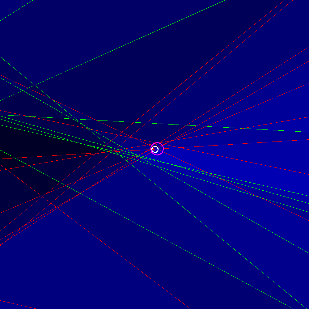
Figure 8: Example of the depth (and maximum depth) for ${\varepsilon}=0.001$ and 20 halfplanes (red are down, green are up). The intensity of the color is proportional to the depth. The maximum depth of the naive algorithm is in white, the maximum depth of the primal dual is in pink. The maximum depth here is 15.

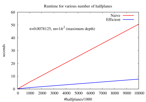
Figure 9: Maximum depth for fixed ${\varepsilon}$ and various $n$

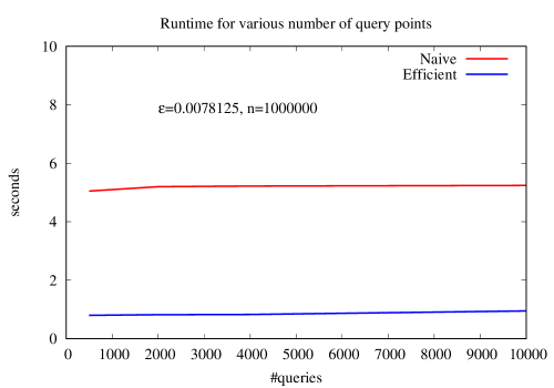
Figure 10: The number of queries is vary for fixed ${\varepsilon}$ and $n$

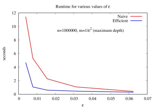
Figure 11: Maximum depth for fixed $n$ and various ${\varepsilon}$ values

References

- [1] Peyman Afshani and Timothy M. Chan. On approximate range counting and depth. Discrete Comput. Geom., 42(1):3–21, 2009.
- [2] Pankaj Agarwal. Simplex range searching and its variants: A review. In M. Loebl, J. Nešetřil, and R. Thomas, editors, A Journey through Discrete Mathematics: A Tribute to Jiri Matousek, pages 1–30. Springer Verlag, Berlin-Heidelberg, 2017.
- [3] Pankaj K. Agarwal and Jeff Erickson. Geometric range searching and its relatives. In B. Chazelle, J.E. Goodman, and R. Pollack, editors, Advances in Discrete and Computational Geometry, pages 1–56. AMS Press, Providence RI, 1998.
- [4] Dror Aiger, Haim Kaplan, Efi Kokiopoulou, Micha Sharir, and Bernhard Zeisl. General techniques for approximate incidences and their application to the camera posing problem. In Proc. 35th Internat. Sympos. Comput. Geom., pages 8:1–8:14, 2019. Also in arXiv:1903.07047.
- [5] Dror Aiger, Haim Kaplan, and Micha Sharir. Output sensitive algorithms for approximate incidences and their applications. In Proc. European Sympos. Algorithms, pages 1–13, 2017.
- [6] Boris Aronov and Sariel Har-Peled. On approximating the depth and related problems. SIAM J. Comput., 38(3):899–921, 2008.
- [7] Sunil Arya and David M. Mount. Approximate range searching. Comput. Geom., 17(3-4):135–152, 2000.
- [8] Robert C. Bolles and Martin A. Fischler. A RANSAC-based approach to model fitting and its application to finding cylinders in range data. In Proc. 7th Internat. Joint Conf. Artificial Intelligence, pages 637–643, 1981.
- [9] Thomas M. Breuel. Implementation techniques for geometric branch-and-bound matching methods. Computer Vision and Image Understanding, 90(3):258–294, 2003.
- [10] Timothy M. Chan. Fixed-dimensional linear programming queries made easy. In Proc. 12th ACM Sympos. Comput. Geom., pages 284–290, 1996.
- [11] Guilherme D. Da Fonseca and David M. Mount. Approximate range searching: The absolute model. Comput. Geom., 43(4):434–444, 2010.
- [12] Johan Fredriksson, Viktor Larsson, and Carl Olsson. Practical robust two-view translation estimation. In Proc. IEEE Conference on Computer Vision and Pattern Recognition, pages 2684–2690, 2015.
- [13] Johan Fredriksson, Viktor Larsson, Carl Olsson, and Fredrik Kahl. Optimal relative pose with unknown correspondences. In Proc. IEEE Conference on Computer Vision and Pattern Recognition, pages 1728–1736, 2016.
- [14] Sariel Har-Peled. Geometric Approximation Algorithms. AMS Press, Providence RI, 2011.
- [15] Sariel Har-Peled and Yusu Wang. Shape fitting with outliers. SIAM J. Comput., 33(2):269–285, 2004.
- [16] David Haussler and Emo Welzl. -nets and simplex range queries. Discrete Comput. Geom., 2(2):127–151, 1987.
- [17] Haim Kaplan, Edgar Ramos, and Micha Sharir. Range minima queries with respect to a random permutation, and approximate range counting. Discrete Comput. Geom., 45(1):3–33, 2011.
- [18] Carl Olsson, Fredrik Kahl, and Magnus Oskarsson. Branch and bound methods for euclidean registration problems. IEEE Trans. Pattern Anal. Mach. Intell., 31(5):783–794, 2009.