1

Deep Network with Approximation Error Being Reciprocal of Width to Power of Square Root of Depth

Zuowei Shen
matzuows@nus.edu.sg
Department of Mathematics, National University of Singapore
 
Haizhao Yang
haizhao@purdue.edu
Department of Mathematics, Purdue University
 
Shijun Zhang
zhangshijun@u.nus.edu
Department of Mathematics, National University of Singapore

Keywords: Exponential Convergence, Curse of Dimensionality, Deep Neural Network, Floor and ReLU Activation Functions, Continuous Function.

A new network with super approximation power is introduced. This network is built with Floor ($\lfloor x\rfloor$) or ReLU ($\max\{0,x\}$) activation function in each neuron and hence we call such networks Floor-ReLU networks. For any hyper-parameters $N\in\mathbb{N}^{+}$ and $L\in\mathbb{N}^{+}$, it is shown that Floor-ReLU networks with width $\max\{d,\,5N+13\}$ and depth $64dL+3$ can uniformly approximate a Hölder function $f$ on $[0,1]^{d}$ with an approximation error $3\lambda d^{\alpha/2}N^{-\alpha\sqrt{L}}$, where $\alpha\in(0,1]$ and $\lambda$ are the Hölder order and constant, respectively. More generally for an arbitrary continuous function $f$ on $[0,1]^{d}$ with a modulus of continuity $\omega_{f}(\cdot)$, the constructive approximation rate is $\omega_{f}(\sqrt{d}\,N^{-\sqrt{L}})+2\omega_{f}(\sqrt{d}){N^{-\sqrt{L}}}$. As a consequence, this new class of networks overcomes the curse of dimensionality in approximation power when the variation of $\omega_{f}(r)$ as $r\to 0$ is moderate (e.g., $\omega_{f}(r)\lesssim r^{\alpha}$ for Hölder continuous functions), since the major term to be considered in our approximation rate is essentially $\sqrt{d}$ times a function of $N$ and $L$ independent of $d$ within the modulus of continuity.

1 Introduction

Recently, there has been a large number of successful real-world applications of deep neural networks in many fields of computer science and engineering, especially for large-scale and high-dimensional learning problems. Understanding the approximation capacity of deep neural networks has become a fundamental research direction for revealing the advantages of deep learning compared to traditional methods. This paper introduces new theories and network architectures achieving root exponential convergence and avoiding the curse of dimensionality simultaneously for (Hölder) continuous functions with an explicit error bound in deep network approximation, which might be two foundational laws supporting the application of deep network approximation in large-scale and high-dimensional problems. The approximation results here are quantitative and apply to networks with essentially arbitrary width and depth. These results suggest considering Floor-ReLU networks as a possible alternative to ReLU networks in deep learning.

Deep ReLU networks with width ${\mathcal{O}}(N)$ and depth ${\mathcal{O}}(L)$ can achieve the approximation rate ${\mathcal{O}}(N^{-L})$ for polynomials on $[0,1]^{d}$ (Lu et al.,, 2020) but it is not true for general functions, e.g., the (nearly) optimal approximation rates of deep ReLU networks for a Lipschitz continuous function and a $C^{s}$ function $f$ on $[0,1]^{d}$ are ${\mathcal{O}}(\sqrt{d}N^{-2/d}L^{-2/d})$ and ${\mathcal{O}}(\|f\|_{C^{s}}N^{-2s/d}L^{-2s/d})$ (Shen et al., 2019b, ; Lu et al.,, 2020), respectively. The limitation of ReLU networks motivates us to explore other types of network architectures to answer our curiosity on deep networks: Do deep neural networks with arbitrary width ${\mathcal{O}}(N)$ and arbitrary depth ${\mathcal{O}}(L)$ admit an exponential approximation rate ${\mathcal{O}}(\omega_{f}(N^{-L^{\eta}}))$ for some constant $\eta>0$ for a generic continuous function $f$ on $[0,1]^{d}$ with a modulus of continuity $\omega_{f}(\cdot)$?

To answer this question, we introduce the Floor-ReLU network, which is a fully connected neural network (FNN) built with either Floor ($\lfloor x\rfloor$) or ReLU ($\max\{0,x\}$) activation function in each neuron. Mathematically, if we let $N_{0}=d$, $N_{L+1}=1$, and $N_{\ell}$ be the number of neurons in $\ell$-th hidden layer of a Floor-ReLU network for $\ell=1,2,\cdots,L$, then the architecture of this network with input ${\bm{x}}$ and output $\phi({\bm{x}})$ can be described as

$${\bm{x}}=\widetilde{\bm{h}}_{0}\mathop{\raisebox{0.0pt}{\scalebox{1.85}[1.0]{$\longrightarrow$}}}^{{\bm{W}}_{0},\,\bm{b}_{0}}\bm{h}_{1}\mathop{\raisebox{0.0pt}{\scalebox{1.8765}[1.0]{$\longrightarrow$}}}^{\textnormal{$\sigma$ or $\lfloor\cdot\rfloor$}}\widetilde{\bm{h}}_{1}\quad\cdots\quad\mathop{\raisebox{0.0pt}{\scalebox{2.54}[1.0]{$\longrightarrow$}}}^{{\bm{W}}_{L-1},\,\bm{b}_{L-1}}\bm{h}_{L}\mathop{\raisebox{0.0pt}{\scalebox{1.8765}[1.0]{$\longrightarrow$}}}^{\textnormal{$\sigma$ or $\lfloor\cdot\rfloor$}}\widetilde{\bm{h}}_{L}\mathop{\raisebox{0.0pt}{\scalebox{1.852}[1.0]{$\longrightarrow$}}}^{{\bm{W}}_{L},\,\bm{b}_{L}}\bm{h}_{L+1}=\phi({\bm{x}}),$$

where ${\bm{W}}_{\ell}\in\mathbb{R}^{N_{\ell+1}\times N_{\ell}}$, $\bm{b}_{\ell}\in\mathbb{R}^{N_{\ell+1}}$, $\bm{h}_{\ell+1}:={\bm{W}}_{\ell}\cdot\widetilde{\bm{h}}_{\ell}+\bm{b}_{\ell}$ for $\ell=0,1,\cdots,L$, and $\widetilde{\bm{h}}_{\ell,n}$ is equal to $\sigma(\bm{h}_{\ell,n})\textnormal{ or }\lfloor\bm{h}_{\ell,n}\rfloor$ for $\ell=1,2,\cdots,L$ and $n=1,2,\cdots,N_{\ell}$, where $\bm{h}_{\ell}=(\bm{h}_{\ell,1},\cdots,\bm{h}_{\ell,N_{\ell}})$ and $\widetilde{\bm{h}}_{\ell}=(\widetilde{\bm{h}}_{\ell,1},\cdots,\widetilde{\bm{h}}_{\ell,N_{\ell}})$ for $\ell=1,2,\cdots,L$. See Figure 1 for an example.

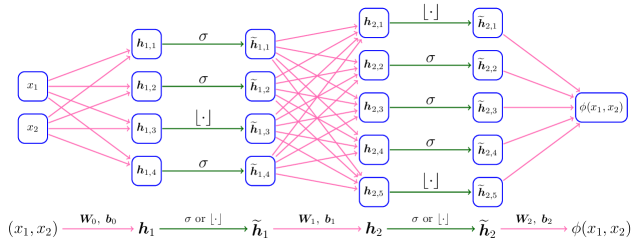
Figure 1: An example of a Floor-ReLU network with width $5$ and depth $2$.

In Theorem 1.1 below, we show by construction that Floor-ReLU networks with width $\max\{d,\,5N+13\}$ and depth $64dL+3$ can uniformly approximate a continuous function $f$ on $[0,1]^{d}$ with a root exponential approximation rate $\omega_{f}(\sqrt{d}\,N^{-\sqrt{L}})+2\omega_{f}(\sqrt{d}){N^{-\sqrt{L}}}$, where $\omega_{f}(\cdot)$ is the modulus of continuity defined as

$$\omega_{f}(r)\coloneqq\sup\big{\{}|f({\bm{x}})-f({\bm{y}})|:\|{\bm{x}}-{\bm{y}}\|_{2}\leq r,\ {\bm{x}},{\bm{y}}\in[0,1]^{d}\big{\}},\quad\textnormal{for any $r\geq 0$,}$$

where $\|{\bm{x}}\|_{2}=\sqrt{x_{1}^{2}+x_{2}^{2}+\cdots+x_{d}^{2}}$ for any ${\bm{x}}=(x_{1},x_{2},\cdots,x_{d})\in\mathbb{R}^{d}$.

Theorem 1.1.

Given any $N,L\in\mathbb{N}^{+}$ and an arbitrary continuous function $f$ on $[0,1]^{d}$, there exists a function $\phi$ implemented by a Floor-ReLU network with width $\max\{d,\,5N+13\}$ and depth $64dL+3$ such that

$$|\phi({\bm{x}})-f({\bm{x}})|\leq\omega_{f}(\sqrt{d}\,N^{-\sqrt{L}})+2\omega_{f}(\sqrt{d}){N^{-\sqrt{L}}},\quad\textnormal{for any ${\bm{x}}\in[0,1]^{d}$.}$$

With Theorem 1.1, we have an immediate corollary.

Corollary 1.2.

Given an arbitrary continuous function $f$ on $[0,1]^{d}$, there exists a function $\phi$ implemented by a Floor-ReLU network with width ${\bar{N}}$ and depth ${\bar{L}}$ such that

$${|\phi({\bm{x}})-f({\bm{x}})|\leq\omega_{f}\Big{(}\sqrt{d}\,{\big{\lfloor}\tfrac{{\bar{N}}-13}{5}\big{\rfloor}}^{-\sqrt{\big{\lfloor}\tfrac{{\bar{L}}-3}{64d}\big{\rfloor}}}\Big{)}+2\omega_{f}(\sqrt{d}){{\big{\lfloor}\tfrac{{\bar{N}}-13}{5}\big{\rfloor}}^{-\sqrt{\big{\lfloor}\tfrac{{\bar{L}}-3}{64d}\big{\rfloor}}}},}$$

for any ${\bm{x}}\in[0,1]^{d}$ and ${\bar{N}},{\bar{L}}\in\mathbb{N}^{+}$ with ${\bar{N}}\geq\max\{d,18\}$ and ${\bar{L}}\geq 64d+3$.

In Theorem 1.1, the rate in $\omega_{f}(\sqrt{d}\,N^{-\sqrt{L}})$ implicitly depends on $N$ and $L$ through the modulus of continuity of $f$, while the rate in $2\omega_{f}(\sqrt{d}){N^{-\sqrt{L}}}$ is explicit in $N$ and $L$. Simplifying the implicit approximation rate to make it explicitly depending on $N$ and $L$ is challenging in general. However, if $f$ is a Hölder continuous function on $[0,1]^{d}$ of order $\alpha\in(0,1]$ with a constant $\lambda$, i.e., $f({\bm{x}})$ satisfying

$$|f({\bm{x}})-f({\bm{y}})|\leq\lambda\|{\bm{x}}-{\bm{y}}\|_{2}^{\alpha},\quad\textnormal{for any ${\bm{x}},{\bm{y}}\in[0,1]^{d}$,}$$ (1)

then $\omega_{f}(r)\leq\lambda r^{\alpha}$ for any $r\geq 0$. Therefore, in the case of Hölder continuous functions, the approximation rate is simplified to $3\lambda d^{\alpha/2}N^{-\alpha\sqrt{L}}$ as shown in the following corollary. In the special case of Lipschitz continuous functions with a Lipschitz constant $\lambda$, the approximation rate is simplified to $3\lambda\sqrt{d}N^{-\sqrt{L}}$.

Corollary 1.3.

Given any $N,L\in\mathbb{N}^{+}$ and a Hölder continuous function $f$ on $[0,1]^{d}$ of order $\alpha$ with a constant $\lambda$, there exists a function $\phi$ implemented by a Floor-ReLU network with width $\max\{d,\,5N+13\}$ and depth $64dL+3$ such that

$$|\phi({\bm{x}})-f({\bm{x}})|\leq 3\lambda d^{\alpha/2}{N^{-\alpha\sqrt{L}}},\quad\textnormal{for any ${\bm{x}}\in[0,1]^{d}$.}$$

First, Theorem 1.1 and Corollary 1.3 show that the approximation capacity of deep networks for continuous functions can be nearly exponentially improved by increasing the network depth, and the approximation error can be explicitly characterized in terms of the width ${\mathcal{O}}(N)$ and depth ${\mathcal{O}}(L)$. Second, this new class of networks overcomes the curse of dimensionality in the approximation power when the modulus of continuity is moderate, since the approximation order is essentially $\omega_{f}(\sqrt{d}N^{-\sqrt{L}})$. Finally, applying piecewise constant and integer-valued functions as activation functions and integer numbers as parameters has been explored in the study of quantized neural networks (Hubara et al.,, 2017; Yin et al.,, 2019; Bengio et al.,, 2013) with efficient training algorithms for low computational complexity (Wang et al.,, 2018). The floor function ($\lfloor x\rfloor$) is a piecewise constant function and can be easily implemented numerically at very little cost. Hence, the evaluation of the proposed network could be efficiently implemented in practical computation. Though there might not be an existing optimization algorithm to identify an approximant with the approximation rate in this paper, Theorem 1.1 can provide an expected accuracy before a learning task and how much the current optimization algorithms could be improved. Designing an efficient optimization algorithm for Floor-ReLU networks will be left as future work with several possible directions discussed later.

We would like to remark that an increased smoothness or regularity of the target function could improve our approximation rate but at the cost of a large prefactor. For example, to attain better approximation rates for functions in $C^{s}([0,1]^{d})$, it is common to use Taylor expansions and derivatives, which are tools that suffer from the curse of dimensionality and will result in a large prefactor like ${\mathcal{O}}((s+1)^{d})$ that is subject to the curse of dimensionality. Furthermore, the prospective approximation rate using smoothness is not attractive. For example, the prospective approximation rate would be ${\mathcal{O}}(N^{-s\sqrt{L}})$, if we use Floor-ReLU networks with width ${\mathcal{O}}(N)$ and depth ${\mathcal{O}}(L)$ to approximate functions in $C^{s}([0,1]^{d})$. However, such a rate ${\mathcal{O}}(N^{-s\sqrt{L}})={\mathcal{O}}(N^{-\sqrt{s^{2}L}})$ can be attained by using Floor-ReLU networks with width ${\mathcal{O}}(N)$ and depth ${\mathcal{O}}(s^{2}L)$ to approximate Lipschitz continuous functions. Hence, increasing the network depth can result in the same approximation rate for Lipschitz continuous functions as the rate of smooth functions.

The rest of this paper is organized as follows. In Section 2, we discuss the application scope of our theory and compare related works in the literature. In Section 3, we prove Theorem 1.1 based on Proposition 3.2. Next, this basic proposition is proved in Section 4. Finally, we conclude this paper in Section 5.

2 Discussion

In this section, we will discuss the application scope of our theory in machine learning and its comparison related to existing works.

2.1 Application scope of our theory in machine learning

In supervised learning, an unknown target function $f(\bm{x})$ defined on a domain $\Omega$ is learned through its finitely many samples $\{(\bm{x}_{i},f(\bm{x}_{i}){)}\}_{i=1}^{n}$. If deep networks are applied in supervised learning, the following optimization problem is solved to identify a deep network $\phi(\bm{x};\bm{\theta}_{\mathcal{S}})$, with $\bm{\theta}_{\mathcal{S}}$ as the set of parameters, to infer $f(\bm{x})$ for unseen data samples $\bm{x}$:

$$\bm{\theta}_{\mathcal{S}}=\operatorname*{arg\,min}_{\bm{\theta}}R_{\mathcal{S}}(\bm{\theta}):=\operatorname*{arg\,min}_{\bm{\theta}}\frac{1}{n}\sum_{\{\bm{x}_{i}\}_{i=1}^{n}}\ell\big{(}\phi(\bm{x}_{i};\bm{\theta}),f(\bm{x}_{i})\big{)}$$ (2)

with a loss function typically taken as $\ell(y,y^{\prime})=\frac{1}{2}|y-y^{\prime}|^{2}$. The inference error is usually measured by $R_{\mathcal{D}}(\bm{\theta}_{\mathcal{S}})$, where

$$R_{\mathcal{D}}(\bm{\theta}):=\textnormal{E}_{\bm{x}\sim U(\Omega)}\left[\ell(\phi(\bm{x};\bm{\theta}),f(\bm{x}))\right],$$

where the expectation is taken with an unknown data distribution $U(\Omega)$ over $\Omega$.

Note that the best deep network to infer $f(\bm{x})$ is $\phi(\bm{x};\bm{\theta}_{\mathcal{D}})$ with $\bm{\theta}_{\mathcal{D}}$ given by

$$\bm{\theta}_{\mathcal{D}}=\operatorname*{arg\,min}_{\bm{\theta}}R_{\mathcal{D}}(\bm{\theta}).$$

The best possible inference error is $R_{\mathcal{D}}(\bm{\theta}_{\mathcal{D}})$. In real applications, $U(\Omega)$ is unknown and only finitely many samples from this distribution are available. Hence, the empirical loss $R_{\mathcal{S}}(\bm{\theta})$ is minimized hoping to obtain $\phi(\bm{x};\bm{\theta}_{\mathcal{S}})$, instead of minimizing the population loss $R_{\mathcal{D}}(\bm{\theta})$ to obtain $\phi(\bm{x};\bm{\theta}_{\mathcal{D}})$. In practice, a numerical optimization method to solve (2) may result in a numerical solution (denoted as $\bm{\theta}_{\mathcal{N}}$) that may not be a global minimizer $\bm{\theta}_{\mathcal{S}}$. Therefore, the actually learned neural network to infer $f(\bm{x})$ is $\phi(\bm{x};\bm{\theta}_{\mathcal{N}})$ and the corresponding inference error is measured by $R_{\mathcal{D}}(\bm{\theta}_{\mathcal{N}})$.

By the discussion just above, it is crucial to quantify $R_{\mathcal{D}}(\bm{\theta}_{\mathcal{N}})$ to see how good the learned neural network $\phi(\bm{x};\bm{\theta}_{\mathcal{N}})$ is, since $R_{\mathcal{D}}(\bm{\theta}_{\mathcal{N}})$ is the expected inference error over all possible data samples. Note that

$$\quad R_{\mathcal{D}}(\bm{\theta}_{\mathcal{N}}) =[R_{\mathcal{D}}(\bm{\theta}_{\mathcal{N}})-R_{\mathcal{S}}(\bm{\theta}_{\mathcal{N}})]+[R_{\mathcal{S}}(\bm{\theta}_{\mathcal{N}})-R_{\mathcal{S}}(\bm{\theta}_{\mathcal{S}})]+[R_{\mathcal{S}}(\bm{\theta}_{\mathcal{S}})-R_{\mathcal{S}}(\bm{\theta}_{\mathcal{D}})]$$

$$\quad+[R_{\mathcal{S}}(\bm{\theta}_{\mathcal{D}})-R_{\mathcal{D}}(\bm{\theta}_{\mathcal{D}})]+R_{\mathcal{D}}(\bm{\theta}_{\mathcal{D}})$$

$$\begin{split}&\leq R_{\mathcal{D}}(\bm{\theta}_{\mathcal{D}})+[R_{\mathcal{S}}(\bm{\theta}_{\mathcal{N}})-R_{\mathcal{S}}(\bm{\theta}_{\mathcal{S}})]\\ &\quad+[R_{\mathcal{D}}(\bm{\theta}_{\mathcal{N}})-R_{\mathcal{S}}(\bm{\theta}_{\mathcal{N}})]+[R_{\mathcal{S}}(\bm{\theta}_{\mathcal{D}})-R_{\mathcal{D}}(\bm{\theta}_{\mathcal{D}})],\end{split}$$ (3)

where the inequality comes from the fact that $[R_{\mathcal{S}}(\bm{\theta}_{\mathcal{S}})-R_{\mathcal{S}}(\bm{\theta}_{\mathcal{D}})]\leq 0$ since $\bm{\theta}_{\mathcal{S}}$ is a global minimizer of $R_{\mathcal{S}}(\bm{\theta})$. The constructive approximation established in this paper and in the literature provides an upper bound of $R_{\mathcal{D}}(\bm{\theta}_{\mathcal{D}})$ in terms of the network size, e.g., in terms of the network width and depth, or in terms of the number of parameters. The second term of (2.1) is bounded by the optimization error of the numerical algorithm applied to solve the empirical loss minimization problem in (2). If the numerical algorithm is able to find a global minimizer, the second term is equal to zero. The theoretical guarantee of the convergence of an optimization algorithm to a global minimizer $\bm{\theta}_{\mathcal{S}}$ and the characterization of the convergence belong to the optimization analysis of neural networks. The third and fourth term of (2.1) are usually bounded in terms of the sample size $n$ and a certain norm of $\bm{\theta}_{\mathcal{N}}$ and $\bm{\theta}_{\mathcal{D}}$ (e.g., $\ell_{1}$, $\ell_{2}$, or the path norm), respectively. The study of the bounds for the third and fourth terms is referred to as the generalization error analysis of neural networks.

The approximation theory, the optimization theory, and the generalization theory form the three main theoretical aspects of deep learning with different emphases and challenges, which have motivated many separate research directions recently. Theorem 1.1 and Corollary 1.3 provide an upper bound of $R_{\mathcal{D}}(\bm{\theta}_{\mathcal{D}})$. This bound only depends on the given budget of neurons and layers of Floor-ReLU networks and on the modulus of continuity of the target function $f$. Hence, this bound is independent of the empirical loss minimization in (2) and the optimization algorithm used to compute the numerical solution of (2). In other words, Theorem 1.1 and Corollary 1.3 quantify the approximation power of Floor-ReLU networks with a given size. Designing efficient optimization algorithms and analyzing the generalization bounds for Floor-ReLU networks are two other separate future directions. Although optimization algorithms and generalization analysis are not our focus in this paper, in the next two paragraphs, we discuss several possible research topics in these directions for our Floor-ReLU networks.

In this work, we have not analyzed the feasibility of optimization algorithms for the Floor-ReLU network. Typically, stochastic gradient descent (SGD) is applied to solve a network optimization problem. However, the Floor-ReLU network has piecewise constant activation functions making standard SGD infeasible. There are two possible directions to solve the optimization problem for Floor-ReLU networks: 1) gradient-free optimization methods, e.g., Nelder-Mead method (Nelder and Mead,, 1965), genetic algorithm (Holland,, 1992), simulated annealing (Kirkpatrick et al.,, 1983), particle swarm optimization (Kennedy and Eberhart,, 1995), and consensus-based optimization (Pinnau et al.,, 2017; Carrillo et al.,, 2019); 2) applying optimization algorithms for quantized networks that also have piecewise constant activation functions (Lin et al.,, 2019; Boo et al.,, 2020; Bengio et al.,, 2013; Wang et al.,, 2018; Hubara et al.,, 2017; Yin et al.,, 2019). It would be interesting future work to explore efficient learning algorithms based on the Floor-ReLU network.

Generalization analysis of Floor-ReLU networks is also an interesting future direction. Previous works have shown the generalization power of ReLU networks for regression problems (Jacot et al.,, 2018; Cao and Gu,, 2019; Chen et al., 2019b, ; E et al.,, 2019; E and Wojtowytsch,, 2020) and for solving partial differential equations (Berner et al.,, 2018; Luo and Yang,, 2020). Regularization strategies for ReLU networks to guarantee good generalization capacity of deep learning have been proposed in (E et al.,, 2019; E and Wojtowytsch,, 2020). It is important to investigate the generalization capacity of our Floor-ReLU networks. Especially, it is of great interest to see whether problem-dependent regularization strategies exist to make the generalization error of our Floor-ReLU networks free of the curse of dimensionality.

2.2 Approximation rates in ${\mathcal{O}}(N)$ and ${\mathcal{O}}(L)$ versus ${\mathcal{O}}(W)$

Characterizing deep network approximation in terms of the width ${\mathcal{O}}(N)$ and depth ${\mathcal{O}}(L)$ simultaneously is fundamental and indispensable in realistic applications, while quantifying the deep network approximation based on the number of nonzero parameters $W$ is probably only of interest in theory as far as we know. Theorem 1.1 can provide practical guidance for choosing network sizes in realistic applications while theories in terms of $W$ cannot tell how large a network should be to guarantee a target accuracy. The width and depth are the two most direct and amenable hyper-parameters in choosing a specific network for a learning task, while the number of nonzero parameters $W$ is hardly controlled efficiently. Theories in terms of $W$ essentially have a single variable to control the network size in three types of structures: 1) fixing the width $N$ and varying the depth $L$; 2) fixing the depth $L$ and changing the width $N$; 3) both the width and depth are controlled by the same parameter like the target accuracy $\varepsilon$ in a specific way (e.g., $N$ is a polynomial of $\frac{1}{\varepsilon^{d}}$ and $L$ is a polynomial of $\log(\frac{1}{\varepsilon})$). Considering the non-uniqueness of structures for realizing the same $W$, it is impractical to develop approximation rates in terms of $W$ covering all these structures. If one network structure has been chosen in a certain application, there might not be a known theory in terms of $W$ to quantify the performance of this structure. Finally, in terms of full error analysis of deep learning including approximation theory, optimization theory, and generalization theory as illustrated in (2.1), the approximation error characterization in terms of width and depth is more useful than that in terms of the number of parameters, because almost all existing optimization and generalization analysis are based on depth and width instead of the number of parameters (Jacot et al.,, 2018; Cao and Gu,, 2019; Chen et al., 2019b, ; Arora et al.,, 2019; Allen-Zhu et al.,, 2019; E et al.,, 2019; E and Wojtowytsch,, 2020; Ji and Telgarsky,, 2020), to the best of our knowledge. Approximation results in terms of width and depth are more consistent with optimization and generalization analysis tools to obtain a full error analysis in (2.1).

Most existing approximation theories for deep neural networks so far focus on the approximation rate in the number of parameters $W$ (Cybenko,, 1989; Hornik et al.,, 1989; Barron,, 1993; Liang and Srikant,, 2016; Yarotsky,, 2017; Poggio et al.,, 2017; E and Wang,, 2018; Petersen and Voigtlaender,, 2018; Chui et al.,, 2018; Yarotsky,, 2018; Nakada and Imaizumi,, 2019; Gribonval et al.,, 2019; Gühring et al.,, 2019; Chen et al., 2019a, ; Li et al.,, 2019; Suzuki,, 2019; Bao et al.,, 2019; Opschoor et al.,, 2019; Yarotsky and Zhevnerchuk,, 2019; Bölcskei et al.,, 2019; Montanelli and Du,, 2019; Chen and Wu,, 2019; Zhou,, 2020; Montanelli and Yang,, 2020; Montanelli et al.,, 2020). From the point of view of theoretical difficulty, controlling two variables $N$ and $L$ in our theory is more challenging than controlling one variable $W$ in the literature. In terms of mathematical logic, the characterization of deep network approximation in terms of $N$ and $L$ can provide an approximation rate in terms of $W$, while we are not aware of how to derive approximation rates in terms of arbitrary $N$ and $L$ given approximation rates in terms of $W$, since existing results in terms of $W$ are valid for specific network sizes with width and depth as functions in $W$ without the degree of freedom to take arbitrary values. As we have discussed in the last paragraph, existing theories essentially have a single variable to control the network size in three types of structures. Let us use the first type of structures, which includes the best-known result for a nearly optimal approximation rate, ${\mathcal{O}}(\omega_{f}(W^{-2/d}))$, for continuous functions in terms of $W$ using ReLU networks (Yarotsky,, 2018) and the best-known result, ${\mathcal{O}}(\text{exp}(-c_{\alpha,d}\sqrt{W}))$, for Hölder continuous functions of order $\alpha$ using Sine-ReLU networks (Yarotsky and Zhevnerchuk,, 2019), as an example to show how Theorem 1.1 in terms of $N$ and $L$ can be applied to show a better result in terms of $W$. One can apply Theorem 1.1 in a similar way to obtain other corollaries with other types of structures in terms of $W$. The main idea is to specify the value of $N$ and $L$ in Theorem 1.1 to show the desired corollary. For example, if we let the width parameter $N=2$ and the depth parameter $L=W$ in Theorem 1.1, then the width is $\max\{d,23\}$, the depth is $64dW+3$, and the total number of parameters is bounded by ${\mathcal{O}}\left(\max\{d^{2},23^{2}\}(64dW+3)\right)={\mathcal{O}}(W)$. Therefore, we can prove Corollary 2.1 below for the approximation capacity of our Floor-ReLU networks in terms of the total number of parameters as follows.

Corollary 2.1.

Given any $W\in\mathbb{N}^{+}$ and a continuous function $f$ on $[0,1]^{d}$, there exists a function $\phi$ implemented by a Floor-ReLU network with ${\mathcal{O}}(W)$ nonzero parameters, a width $\max\{d,\,23\}$ and depth $64dW+3$, such that

$$|\phi({\bm{x}})-f({\bm{x}})|\leq\omega_{f}(\sqrt{d}\,2^{-\sqrt{W}})+2\omega_{f}(\sqrt{d}){2^{-\sqrt{W}}},\quad\textnormal{for any ${\bm{x}}\in[0,1]^{d}$.}$$

Corollary 2.1 achieves root exponential convergence without the curse of dimensionality in terms of the number of parameters $W$ with the help of the Floor-ReLU networks. When only ReLU networks are used, the result in (Yarotsky,, 2018) suffers from the curse and does not have any kind of exponential convergence. The result in (Yarotsky and Zhevnerchuk,, 2019) with Sine-ReLU networks has root exponential convergence but has not excluded the possibility of the curse of dimensionality as we shall discuss later. Furthermore, Corollary 2.1 works for generic continuous functions while (Yarotsky and Zhevnerchuk,, 2019) only applies to Hölder continuous functions.

2.3 Further interpretation of our theory

In the interpretation of our theory, there are two more aspects that are important to discuss. The first one is whether it is possible to extend our theory to functions on a more general domain, e.g, $[-M,M]^{d}$ for some $M>1$, because $M>1$ may cause an implicit curse of dimensionality in some existing theory as we shall point out later. The second one is how bad the modulus of continuity would be since it is related to a high-dimensional function $f$ that may lead to an implicit curse of dimensionality in our approximation rate.

First, Theorem 1.1 can be easily generalized to $C([-M,M]^{d})$ for any $M>0$. Let ${\mathcal{L}}$ be a linear map given by ${\mathcal{L}}({\bm{x}})=2M({\bm{x}}-1/2)$. By Theorem 1.1, for any $f\in C([-M,M]^{d})$, there exists $\phi$ implemented by a Floor-ReLU network with width $\max\{d,\,5N+13\}$ and depth $64dL+3$ such that

$$|\phi({\bm{x}})-f\circ{\mathcal{L}}({\bm{x}})|\leq\omega_{f\circ{\mathcal{L}}}(\sqrt{d}\,N^{-\sqrt{L}})+2\omega_{f\circ{\mathcal{L}}}(\sqrt{d}){N^{-\sqrt{L}}},\quad\textnormal{for any ${\bm{x}}\in[0,1]^{d}$.}$$

It follows from ${\bm{y}}={\mathcal{L}}({\bm{x}})\in[-M,M]^{d}$ and $\omega_{f\circ{\mathcal{L}}}{(r)}=\omega_{f}^{\scriptscriptstyle[-M,M]^{d}}(2Mr)$ for any $r\geq 0$ that, for any ${\bm{y}}\in[-M,M]^{d}$,

$$|\phi(\tfrac{{\bm{y}}+M}{2M})-f({\bm{y}})|\leq\omega_{f}^{\scriptscriptstyle[-M,M]^{d}}(2M\sqrt{d}\,N^{-\sqrt{L}})+2\omega_{f}^{\scriptscriptstyle[-M,M]^{d}}(2M\sqrt{d}){N^{-\sqrt{L}}}.$$ (4)

Hence, the size of the function domain $[-M,M]^{d}$ only has a mild influence on the approximation rate of our Floor-ReLU networks. Floor-ReLU networks can still avoid the curse of dimensionality and achieve root exponential convergence for continuous functions on $[-M,M]^{d}$ when $M>1$. For example, in the case of Hölder continuous functions of order $\alpha$ with a constant $\lambda$ on $[-M,M]^{d}$, our approximation rate becomes $3\lambda(2M\sqrt{d}{N^{-\sqrt{L}}})^{\alpha}$.

Second, most interesting continuous functions in practice have a good modulus of continuity such that there is no implicit curse of dimensionality hiding in $\omega_{f}(\cdot)$. For example, we have discussed the case of Hölder continuous functions previously. We would like to remark that the class of Hölder continuous functions implicitly depends on $d$ through its definition in (1), but this dependence is moderate since the $\ell^{2}$- norm in (1) is the square root of a sum with $d$ terms. Let us now discuss several cases of $\omega_{f}(\cdot)$ when we cannot achieve exponential convergence or cannot avoid the curse of dimensionality. The first example is $\omega_{f}(r)=\tfrac{1}{\ln(1/r)}$ for all small $r>0$, which leads to an approximation rate

$$3(\sqrt{L}\ln N-\tfrac{1}{2}\ln d)^{-1},\quad\textnormal{for large $N,L\in\mathbb{N}^{+}$}.$$

Apparently, the above approximation rate still avoids the curse of dimensionality but there is no exponential convergence, which has been canceled out by “$\ln$” in $\omega_{f}(\cdot)$. The second example is $\omega_{f}(r)=\tfrac{1}{\ln^{1/d}(1/r)}$ for all small $r>0$, which leads to an approximation rate

$$3(\sqrt{L}\ln N-\tfrac{1}{2}\ln d)^{-1/d},\quad\textnormal{for large $N,L\in\mathbb{N}^{+}$}.$$

The power $\frac{1}{d}$ further weakens the approximation rate and hence the curse of dimensionality occurs. The last example we would like to discuss is $\omega_{f}(r)=r^{\alpha/d}$ for all small $r>0$, which results in the approximation rate

$$3d^{\tfrac{\alpha}{2d}}{N^{-\tfrac{\alpha}{d}\sqrt{L}}},\quad\textnormal{for large $N,L\in\mathbb{N}^{+}$},$$

which achieves the exponential convergence and avoids the curse of dimensionality when we use very deep networks with a fixed width. But if we fix the depth, there is no exponential convergence and the curse occurs. Though we have provided several examples of immoderate $\omega_{f}(\cdot)$, to the best of our knowledge, we are not aware of practically useful continuous functions with $\omega_{f}(\cdot)$ that is immoderate.

2.4 Discussion on the literature

The neural networks constructed here achieve exponential convergence without the curse of dimensionality simultaneously for a function class as general as (Hölder) continuous functions, while–to the best of our knowledge–most existing theories only apply to functions with an intrinsic low complexity. For example, the exponential convergence was studied for polynomials (Yarotsky,, 2017; Montanelli et al.,, 2020; Lu et al.,, 2020), smooth functions (Montanelli et al.,, 2020; Liang and Srikant,, 2016), analytic functions (E and Wang,, 2018), and functions admitting a holomorphic extension to a Bernstein polyellipse (Opschoor et al.,, 2019). For another example, no curse of dimensionality occurs, or the curse is lessened for Barron spaces (Barron,, 1993; E et al.,, 2019; E and Wojtowytsch,, 2020), Korobov spaces (Montanelli and Du,, 2019), band-limited functions (Chen and Wu,, 2019; Montanelli et al.,, 2020), compositional functions (Poggio et al.,, 2017), and smooth functions (Yarotsky and Zhevnerchuk,, 2019; Lu et al.,, 2020; Montanelli and Yang,, 2020; Yang and Wang,, 2020).

Our theory admits a neat and explicit approximation error bound. For example, our approximation rate in the case of Hölder continuous functions of order $\alpha$ with a constant $\lambda$ is $3\lambda d^{\alpha/2}{N^{-\alpha\sqrt{L}}}$, while the prefactor of most existing theories is unknown or grows exponentially in $d$. Our proof fully explores the advantage of the compositional structure and the nonlinearity of deep networks, while many existing theories were built on traditional approximation tools (e.g., polynomial approximation, multiresolution analysis, and Monte Carlo sampling), making it challenging for existing theories to obtain a neat and explicit error bound with an exponential convergence and without the curse of dimensionality.

Let us review existing works in more detail below.

Curse of dimensionality. The curse of dimensionality is the phenomenon that approximating a $d$-dimensional function using a certain parametrization method with a fixed target accuracy generally requires a large number of parameters that is exponential in $d$ and this expense quickly becomes unaffordable when $d$ is large. For example, traditional finite element methods with $W$ parameters can achieve an approximation accuracy $O(W^{-1/d})$ with an explicit indicator of the curse $\frac{1}{d}$ in the power of $W$. If an approximation rate has a constant independent of $W$ and exponential in $d$, the curse still occurs implicitly through this prefactor by definition. If the approximation rate has a prefactor $C_{f}$ depending on $f$, then the prefactor $C_{f}$ still depends on $d$ implicitly via $f$ and the curse implicitly occurs if $C_{f}$ exponentially grows when $d$ increases. Designing a parametrization method that can overcome the curse of dimensionality is an important research topic in approximation theory.

In (Barron,, 1993) and its variants or generalization (E et al.,, 2019; E and Wojtowytsch,, 2020; Chen and Wu,, 2019; Montanelli et al.,, 2020), $d$-dimensional functions defined on a domain $\Omega\subseteq\mathbb{R}^{d}$ admitting an integral representation with an integrand as a ridge function on $\widetilde{\Omega}\subseteq\mathbb{R}^{d}$ with a variable coefficent were considered, e.g.,

$$f({\bm{x}})=\int_{\widetilde{\Omega}}a(\bm{w})K(\bm{w}\cdot{\bm{x}})d\nu(\bm{w}),$$ (5)

where $\nu(\bm{w})$ is a Lebesgue measure in $\bm{w}$. $f({\bm{x}})$ can be reformulated into the expectation of a high-dimensional random function when $\bm{w}$ is treated as a random variable. Then $f({\bm{x}})$ can be approximated by the average of $W$ samples of the integrand in the same spirit of the law of large numbers with an approximation error essentially bounded by $\frac{C_{f}\sqrt{\mu(\Omega)}}{\sqrt{W}}$ measured in $L^{2}(\Omega,\mu)$ (Equation (6) of (Barron,, 1993)), where ${\mathcal{O}}(W)$ is the total number of parameters in the network, $C_{f}$ is a $d$-dimensional integral with an integrand related to $f$, and $\mu(\Omega)$ is the Lebesgue measure of $\Omega$. As pointed out in (Barron,, 1993) right after Equation (6), if $\Omega$ is not a unit domain in $\mathbb{R}^{d}$, $\mu(\Omega)$ would be exponential in $d$; at the beginning of Page 932 of (Barron,, 1993), it was remarked that $C_{f}$ can often be exponentially large in $d$ and standard smoothness properties of $f$ alone are not enough to remove the exponential dependence of $C_{f}$ on $d$, though there is a large number of examples for which $C_{f}$ is only moderately large. Therefore, the curse of dimensionality occurs unless $C_{f}$ and $\mu(\Omega)$ are not exponential in $d$. It was observed that if the error is measured in the sense of mean squared error in machine learning, which is the square of the $L^{2}(\Omega,\mu)$ error averaged over $\mu(\Omega)$ resulting in $\frac{C^{2}_{f}}{W}$, then the mean squared error has no curse of dimensionality as long as $C_{f}$ is not exponential in $d$ (Barron,, 1993; E et al.,, 2019; E and Wojtowytsch,, 2020).

In (Montanelli and Du,, 2019), $d$-dimensional functions in the Korobov space are approximated by the linear combination of basis functions of a sparse grid, each of which is approximated by a ReLU network. Though the curse of dimensionality has been lessened, target functions have to be sufficiently smooth and the approximation error still contains a factor that is exponential in $d$, i.e., the curse still occurs. Other works in (Yarotsky,, 2017; Yarotsky and Zhevnerchuk,, 2019; Lu et al.,, 2020; Yang and Wang,, 2020) study the advantage of smoothness in the network approximation. Polynomials are applied to approximate smooth functions and ReLU networks are constructed to approximate polynomials. The application of smoothness can lessen the curse of dimensionality in the approximation rates in terms of network sizes but also results in a prefactor that is exponentially large in the dimension, which means that the curse still occurs implicitly.

The Kolmogorov-Arnold superposition theorem (KST) (Kolmogorov,, 1956; Arnold,, 1957; Kolmogorov,, 1957) has also inspired a research direction of network approximation (Kůrková,, 1992; Maiorov and Pinkus,, 1999; Igelnik and Parikh,, 2003; Montanelli and Yang,, 2020) for continuous functions. (Kůrková,, 1992) provided a quantitative approximation rate of networks with two hidden layers, but the number of neurons scales exponentially in the dimension and the curse occurs. (Maiorov and Pinkus,, 1999) relaxes the exact representation in KST to an approximation in a form of two-hidden-layer neural networks with a maximum width $6d+3$ and a single activation function. This powerful activation function is very complex as described by its authors and its numerical evaluation was not available until a more concrete algorithm was recently proposed in (Guliyev and Ismailov,, 2018). Note that there is no available numerical algorithm in (Maiorov and Pinkus,, 1999; Guliyev and Ismailov,, 2018) to compute the whole networks proposed therein. The difficulty is due to the fact that the construction of these networks relies on the outer univariate continuous function of the KST. Though the existence of these outer functions can be shown by construction via a complicated iterative procedure in (Braun and Griebel,, 2009), there is no existing numerical algorithm to evaluate them for a given target function yet, even though computation with an arbitrary precision is assumed to be available. Therefore, the networks considered in (Maiorov and Pinkus,, 1999; Guliyev and Ismailov,, 2018) are similar to the original representation in KST in the sense that their existence is proved without an explicit way or numerical algorithm to construct them. (Igelnik and Parikh,, 2003) and (Montanelli and Yang,, 2020) apply cubic-splines and piecewise linear functions to approximate the inner and outer functions of KST, resulting in cubic-spline and ReLU networks to approximate continuous functions on $[0,1]^{d}$. Due to the pathological outer functions of KST, the approximation bounds still suffer from the curse of dimensionality unless target functions are restricted to a small class of functions with simple outer functions in the KST.

Recently in (Yarotsky and Zhevnerchuk,, 2019), Sine-ReLU networks have been applied to approximate Hölder continuous functions of order $\alpha$ on $[0,1]^{d}$ with an approximation accuracy $\varepsilon=\text{exp}(-c_{\alpha,d}W^{1/2})$, where $W$ is the number of parameters in the network and $c_{\alpha,d}$ is a positive constant depending on $\alpha$ and $d$ only. Whether or not $c_{\alpha,d}$ exponentially depends on $d$ determines whether or not the curse of dimensionality exists for the Sine-ReLU networks, which is not answered in (Yarotsky and Zhevnerchuk,, 2019) and is still an open question.

Finally, we would like to discuss the curse of dimensionality in terms of the continuity of the weight selection as a map $\Sigma:C([0,1]^{d})\rightarrow\mathbb{R}^{W}$. For a fixed network architecture with a fixed number of parameters $W$, let $g:\mathbb{R}^{W}\rightarrow C([0,1]^{d})$ be the map of realizing a DNN from a given set of parameters in $\mathbb{R}^{W}$ to a function in $C([0,1]^{d})$. Suppose that there is a continuous map $\Sigma$ from the unit ball of Sobolev space with smoothness $s$, denoted as $F_{s,d}$, to $\mathbb{R}^{W}$ such that $\|f-g(\Sigma(f))\|_{L^{\infty}}\leq\varepsilon$ for all $f\in F_{s,d}$. Then $W\geq c\varepsilon^{-d/s}$ with some constant $c$ depending only on $s$. This conclusion is given in Theorem 3 of (Yarotsky,, 2017), which is a corollary of Theorem 4.2 of (Devore,, 1989) in a more general form. Intuitively, this conclusion means that any constructive approximation of ReLU FNNs to approximate $C([0,1]^{d})$ cannot enjoy a continuous weight selection property if the approximation rate is better than $c\varepsilon^{-d/s}$, i.e., the curse of dimensionality must occur for constructive approximation for ReLU FNNs with a continuous weight selection. Theorem 4.2 of (Devore,, 1989) can also lead to a new corollary with a weight selection map $\Sigma:K_{s,d}\rightarrow\mathbb{R}^{W}$ (e.g., the constructive approximation of Floor-ReLU networks) and $g:\mathbb{R}^{W}\rightarrow L^{\infty}([0,1]^{d})$ (e.g., the realization map of Floor-ReLU networks), where $K_{s,d}$ is the unit ball of $C^{s}([0,1]^{d})$ with the Sobolev norm $W^{s,\infty}([0,1]^{d})$. Then this new corollary implies that the constructive approximation in this paper cannot enjoy continuous weight selection. However, Theorem 4.2 of (Devore,, 1989) is essentially a min-max criterion to evaluate weight selection maps maintaining continuity: the approximation error obtained by minimizing over all continuous selection $\Sigma$ and network realization $g$ and maximizing over all target functions is bounded below by ${\mathcal{O}}(W^{-s/d})$. In the worst scenario, a continuous weight selection cannot enjoy an approximation rate beating the curse of dimensionality. However, Theorem 4.2 of (Devore,, 1989) has not excluded the possibility that most continuous functions of interest in practice may still enjoy a continuous weight selection without the curse of dimensionality.

Exponential convergence. Exponential convergence is referred to as the situation that the approximation error exponentially decays to zero when the number of parameters increases. Designing approximation tools with an exponential convergence is another important topic in approximation theory. In the literature of deep network approximation, when the number of network parameters $W$ is a polynomial of ${\mathcal{O}}(\log(\frac{1}{\varepsilon}))$, the terminology “exponential convergence” was also used (E and Wang,, 2018; Yarotsky and Zhevnerchuk,, 2019; Opschoor et al.,, 2019). The exponential convergence in this paper is root-exponential as in (Yarotsky and Zhevnerchuk,, 2019), i.e., $W={\mathcal{O}}(\log^{2}(\frac{1}{\varepsilon}))$. The exponential convergence in other works is worse than root-exponential.

In most cases, the approximation power to achieve exponential approximation rates in existing works comes from traditional tools for approximating a small class of functions instead of taking advantage of the network structure itself. In (E and Wang,, 2018; Opschoor et al.,, 2019), highly smooth functions are first approximated by the linear combination of special polynomials with high degrees (e.g., Chebyshev polynomials, Legendre polynomials) with an exponential approximation rate, i.e., to achieve an $\varepsilon$-accuracy, a linear combination of only ${\mathcal{O}}(p(\log(\frac{1}{\varepsilon})))$ polynomials is required, where $p$ is a polynomial with a degree that may depend on the dimension $d$. Then each polynomial is approximated by a ReLU network with ${\mathcal{O}}(\log(\frac{1}{\varepsilon}))$ parameters. Finally, all ReLU networks are assembled to form a large network approximating the target function with an exponential approximation rate. As far as we know, the only existing work that achieves exponential convergence without taking advantage of special polynomials and smoothness is the Sine-ReLU network in (Yarotsky and Zhevnerchuk,, 2019), which has been mentioned in the paragraph just above. We would like to emphasize that the result in our paper applies for generic continuous functions including, but not limited to, the Hölder continuous functions considered in (Yarotsky and Zhevnerchuk,, 2019).

3 Approximation of continuous functions

In this section, we first introduce basic notations in this paper in Section 3.1. Then we prove Theorem 1.1 based on Proposition 3.2, which will be proved in Section 4.

3.1 Notations

The main notations of this paper are listed as follows.

• Vectors and matrices are denoted in a bold font. Standard vectorization is adopted in the matrix and vector computation. For example, adding a scalar and a vector means adding the scalar to each entry of the vector.

• Let $\mathbb{N}^{+}$ denote the set containing all positive integers, i.e., $\mathbb{N}^{+}=\{1,2,3,\cdots\}$.

• Let $\sigma:\mathbb{R}\to\mathbb{R}$ denote the rectified linear unit (ReLU), i.e. $\sigma(x)=\max\{0,x\}$. With a slight abuse of notation, we define $\sigma:\mathbb{R}^{d}\to\mathbb{R}^{d}$ as $\sigma({\bm{x}})=\left[\begin{array}[]{c}\max\{0,x_{1}\}\\ \vdots\\ \max\{0,x_{d}\}\end{array}\right]$ for any ${\bm{x}}=(x_{1},\cdots,x_{d})\in\mathbb{R}^{d}$.

• The floor function (Floor) is defined as $\lfloor x\rfloor:=\max\{n:n\leq x,\ n\in\mathbb{Z}\}$ for any $x\in\mathbb{R}$.

• For $\theta\in[0,1)$, suppose its binary representation is $\theta=\sum_{\ell=1}^{\infty}\theta_{\ell}2^{-\ell}$ with $\theta_{\ell}\in\{0,1\}$, we introduce a special notation $\textnormal{bin}\hskip 1.2pt0.\theta_{1}\theta_{2}\cdots\theta_{L}$ to denote the $L$-term binary representation of $\theta$, i.e., ${\textnormal{bin}\hskip 1.2pt0.\theta_{1}\theta_{2}\cdots\theta_{L}\coloneqq}\sum_{\ell=1}^{L}\theta_{\ell}2^{-\ell}$.

• The expression “a network with width $N$ and depth $L$” means

  • The maximum width of this network for all hidden layers is no more than $N$.

  • The number of hidden layers of this network is no more than $L$.

3.2 Proof of Theorem 1.1

Theorem 1.1 is an immediate consequence of Theorem 3.1 below.

Theorem 3.1.

Given any $N,L\in\mathbb{N}^{+}$ and an arbitrary continuous function $f$ on $[0,1]^{d}$, there exists a function $\phi$ implemented by a Floor-ReLU network with width $\max\{d,\,2N^{2}+5N\}$ and depth $7dL^{2}+3$ such that

$$|\phi({\bm{x}})-f({\bm{x}})|\leq\omega_{f}(\sqrt{d}\,N^{-L})+2\omega_{f}(\sqrt{d})2^{-NL},\quad\textnormal{for any ${\bm{x}}\in[0,1]^{d}$.}$$

This theorem will be proved later in this section. Now let us prove Theorem 1.1 based on Theorem 3.1.

Proof of Theorem 1.1.

Given any $N,L\in\mathbb{N}^{+}$, there exist ${\widetilde{N}},{\widetilde{L}}\in\mathbb{N}^{+}$ with ${\widetilde{N}}\geq 2$ and ${\widetilde{L}}\geq 3$ such that

$$({\widetilde{N}}-1)^{2}\leq N<{\widetilde{N}}^{2}\quad\textnormal{and}\quad({\widetilde{L}}-1)^{2}\leq 4L<{\widetilde{L}}^{2}.$$

By Theorem 3.1, there exists a function $\phi$ implemented by a Floor-ReLU network with width $\max\{d,\,2{\widetilde{N}}^{2}+5{\widetilde{N}}\}$ and depth $7d{\widetilde{L}}^{2}+3$ such that

$$|\phi({\bm{x}})-f({\bm{x}})|\leq\omega_{f}(\sqrt{d}\,{\widetilde{N}}^{-{\widetilde{L}}})+2\omega_{f}(\sqrt{d})2^{-{\widetilde{N}}{\widetilde{L}}},\quad\textnormal{for any ${\bm{x}}\in[0,1]^{d}$.}$$

Note that

$$2^{-{\widetilde{N}}{\widetilde{L}}}\leq{\widetilde{N}}^{-{\widetilde{L}}}=({\widetilde{N}}^{2})^{-\tfrac{1}{2}\sqrt{{\widetilde{L}}^{2}}}\leq N^{-\tfrac{1}{2}\sqrt{4L}}\leq N^{-\sqrt{L}}.$$

Then we have

$$|\phi({\bm{x}})-f({\bm{x}})|\leq\omega_{f}(\sqrt{d}\,N^{-\sqrt{L}})+2\omega_{f}(\sqrt{d})N^{-\sqrt{L}},\quad\textnormal{for any ${\bm{x}}\in[0,1]^{d}$.}$$

For ${\widetilde{N}},{\widetilde{L}}\in\mathbb{N}^{+}$ with ${\widetilde{N}}\geq 2$ and ${\widetilde{L}}\geq 3$, we have

$${\color[rgb]{0,0,0}2{\widetilde{N}}^{2}+{5}{\widetilde{N}}\leq 5({\widetilde{N}}-1)^{2}+13\leq 5N+13\quad\textnormal{and}\quad 7{\widetilde{L}}^{2}\leq 16({\widetilde{L}}-1)^{2}\leq 64L.}$$

Therefore, $\phi$ can be computed by a Floor-ReLU network with width $\max\{d,\,2{\widetilde{N}}^{2}+5{\widetilde{N}}\}\leq\max\{d,\,5N+13\}$ and depth $7d{\widetilde{L}}^{2}+3\leq 64dL+3$, as desired. So we finish the proof. ∎

To prove Theorem 3.1, we first present the proof sketch. Put briefly, we construct piecewise constant functions implemented by Floor-ReLU networks to approximate continuous functions. There are four key steps in our construction.

1. Normalize $f$ as ${\widetilde{f}}$ satisfying ${\widetilde{f}}({\bm{x}})\in[0,1]$ for any ${\bm{x}}\in[0,1]^{d}$, divide $[0,1]^{d}$ into a set of non-overlapping cubes $\{Q_{\bm{\beta}}\}_{{\bm{\beta}}\in\{0,1,\cdots,K-1\}^{d}}$, and denote ${\bm{x}}_{\bm{\beta}}$ as the vertex of $Q_{\bm{\beta}}$ with minimum $\|\cdot\|_{1}$ norm, where $K$ is an integer determined later. See Figure 2 for the illustrations of $Q_{\bm{\beta}}$ and ${\bm{x}}_{\bm{\beta}}$.

2. Construct a Floor-ReLU sub-network to implement a vector-valued function $\bm{\Phi}_{1}:\mathbb{R}^{d}\to\mathbb{R}^{d}$ projecting the whole cube $Q_{\bm{\beta}}$ to the index ${\bm{\beta}}$ for each ${\bm{\beta}}\in\{0,1,\cdots,K-1\}^{d}$, i.e., ${\bm{\Phi}}_{1}({\bm{x}})={\bm{\beta}}$ for all ${\bm{x}}\in Q_{\bm{\beta}}$.

3. Construct a Floor-ReLU sub-network to implement a function $\phi_{2}:\mathbb{R}^{d}\to\mathbb{R}$ mapping ${\bm{\beta}}\in\{0,1,\cdots,K-1\}^{d}$ approximately to ${\widetilde{f}}({\bm{x}}_{\bm{\beta}})$ for each ${\bm{\beta}}$, i.e., $\phi_{2}({\bm{\beta}})\approx{\widetilde{f}}({\bm{x}}_{\bm{\beta}})$. Then $\phi_{2}\circ\bm{\Phi}_{1}({\bm{x}})=\phi_{2}({\bm{\beta}})\approx{\widetilde{f}}({\bm{x}}_{\bm{\beta}})$ for any ${\bm{x}}\in Q_{\bm{\beta}}$ and each ${\bm{\beta}}\in\{0,1,\cdots,K-1\}^{d}$, implying ${\widetilde{\phi}}\coloneqq\phi_{2}\circ\bm{\Phi}_{1}$ approximates ${\widetilde{f}}$ within an error ${\mathcal{O}}(\omega_{f}(1/K))$ on $[0,1]^{d}$.

4. Re-scale and shift ${\widetilde{\phi}}$ to obtain the desired function $\phi$ approximating $f$ well and determine the final Floor-ReLU network to implement $\phi$.

It is not difficult to construct Floor-ReLU networks with the desired width and depth to implement $\bm{\Phi}_{1}$. The most technical part is the construction of a Floor-ReLU network with the desired width and depth computing $\phi_{2}$, which needs the following proposition based on the “bit extraction” technique introduced in (Bartlett et al.,, 1998; Harvey et al.,, 2017).

Proposition 3.2.

Given any $N,L\in\mathbb{N}^{+}$ and arbitrary $\theta_{m}\in\{0,1\}$ for $m=1,2,\cdots,N^{L}$, there exists a function $\phi$ computed by a Floor-ReLU network with width $2N+2$ and depth $7L-2$ such that

$$\phi(m)=\theta_{m},\quad\textnormal{for $m={1,2,\cdots,N^{L}}$.}$$

The proof of this proposition is presented in Section 4. By this proposition and the definition of VC-dimension (e.g., see (Harvey et al.,, 2017)), it is easy to prove that the VC-dimension of Floor-ReLU networks with a constant width and depth ${\mathcal{O}}(L)$ has a lower bound $2^{L}$. Such a lower bound is much larger than ${\mathcal{O}}(L^{2})$, which is a VC-dimension upper bound of ReLU networks with the same width and depth due to Theorem 8 of (Harvey et al.,, 2017). This means Floor-ReLU networks are much more powerful than ReLU networks from the perspective of VC-dimension.

Based on the proof sketch stated just above, we are ready to give the detailed proof of Theorem 3.1 following similar ideas as in our previous work (Shen et al., 2019a, ; Shen et al., 2019b, ; Lu et al.,, 2020). The main idea of our proof is to reduce high-dimensional approximation to one-dimensional approximation via a projection. The idea of projection was probably first used in well-established theories, e.g., KST (Kolmogorov superposition theorem) mentioned in Section 2, where the approximant to high-dimensional functions is constructed by: first, projecting high-dimensional data points to one-dimensional data points; second, construct one-dimensional approximants. There has been extensive research based on this idea, e.g., references related to KST summarized in Section 2, our previous works (Shen et al., 2019a, ; Shen et al., 2019b, ; Lu et al.,, 2020), and (Yarotsky and Zhevnerchuk,, 2019). The key to a successful approximant is to construct one-dimensional approximants to deal with a large number of one-dimensional data points; in fact, the number of points is exponential in the dimension $d$.

Proof of Theorem 3.1.

The proof consists of four steps.

Step $1\colon$ Set up.

Assume $f$ is not a constant function since it is a trivial case. Then $\omega_{f}(r)>0$ for any $r>0$. Clearly, $|f({\bm{x}})-f({\bm{0}})|\leq\omega_{f}(\sqrt{d})$ for any ${\bm{x}}\in[0,1]^{d}$. Define

$${\widetilde{f}}\coloneqq\big{(}f-f({\bm{0}})+\omega_{f}(\sqrt{d})\big{)}\big{/}\big{(}2\omega_{f}(\sqrt{d})\big{)}.$$ (6)

It follows that ${\widetilde{f}}({\bm{x}})\in[0,1]$ for any ${\bm{x}}\in[0,1]^{d}$.

Set $K=N^{L}$, $E_{K-1}=[\tfrac{K-1}{K},1]$, and $E_{k}=[\tfrac{k}{K},\tfrac{k+1}{K})$ for $k=0,1,\cdots,K-2$. Define ${\bm{x}}_{\bm{\beta}}\coloneqq{\bm{\beta}}/K$ and

$$Q_{\bm{\beta}}\coloneqq\Big{\{}{\bm{x}}=(x_{1},x_{2},\cdots,x_{d})\in\mathbb{R}^{d}:x_{j}\in E_{\beta_{j}}\ \textnormal{for}\ j=1,2,\cdots,d\Big{\}},$$

for any ${\bm{\beta}}=(\beta_{1},\beta_{2}\cdots,\beta_{d})\in\{0,1,\cdots,K-1\}^{d}$. See Figure 2 for the examples of $Q_{\bm{\beta}}$ and ${\bm{x}}_{\bm{\beta}}$ for ${\bm{\beta}}\in\{0,1,\cdots,K-1\}^{d}$ with $K=4$ and $d=1,2$.

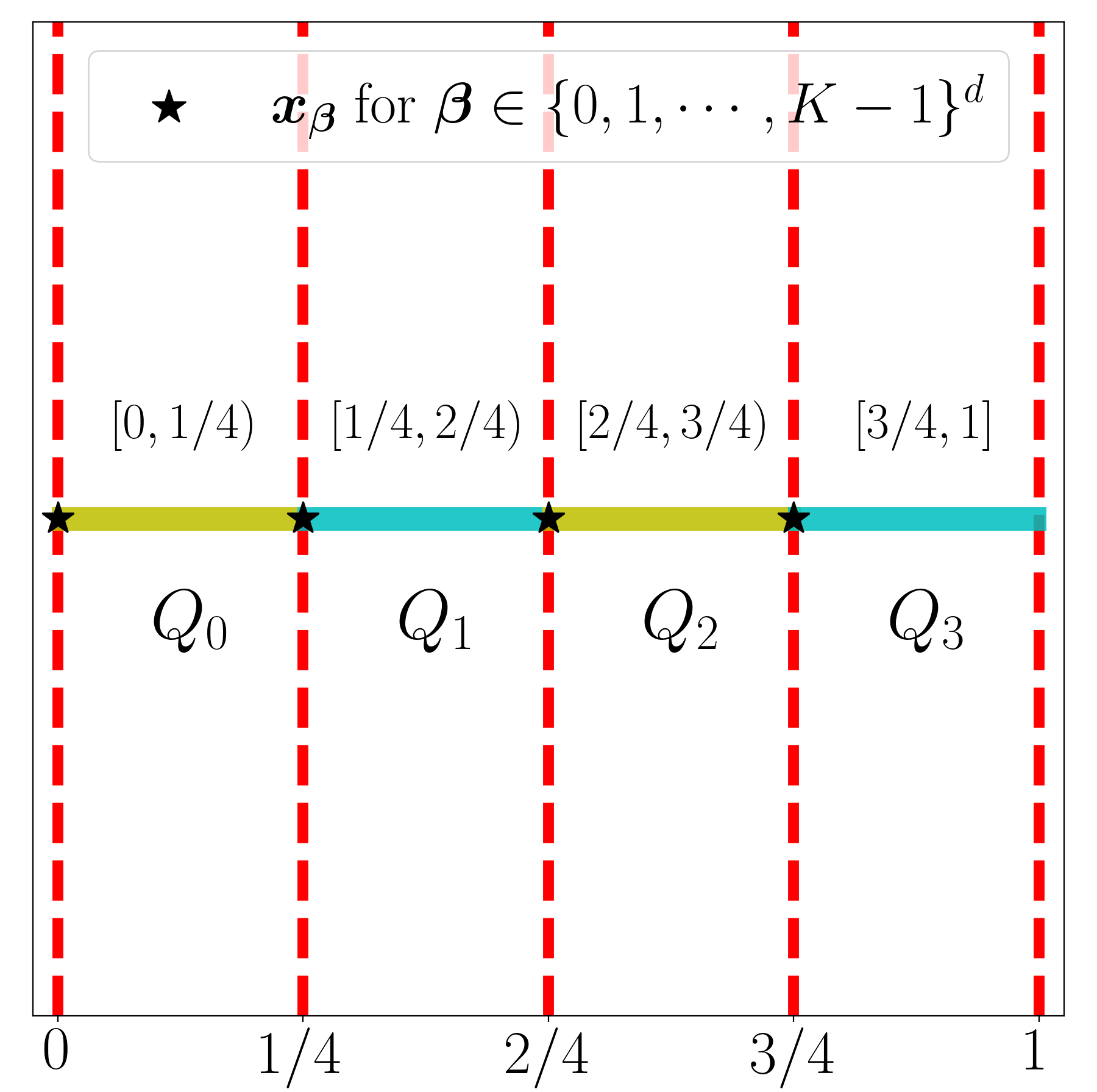
(a)

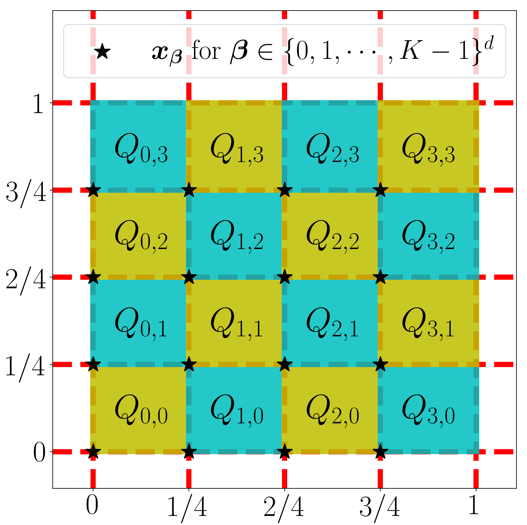
(b)

Figure 2: Illustrations of $Q_{\bm{\beta}}$ and ${\bm{x}}_{\bm{\beta}}$ for ${\bm{\beta}}\in\{0,1,\cdots,K-1\}^{d}$. (a) $K=4,\ d=1$. (b) $K=4,\ d=2$.

Step $2\colon$ Construct $\bm{\Phi}_{1}$ mapping ${\bm{x}}\in Q_{\bm{\beta}}$ to ${\bm{\beta}}$.

Define a step function $\phi_{1}$ as

$$\phi_{1}(x)\coloneqq\big{\lfloor}-\sigma(-Kx+K-1)+K-1\big{\rfloor},\quad\textnormal{for any $x\in\mathbb{R}$.}$$

See Figure 3 for an example of $\phi_{1}$ when $K=4$. It follows from the definition of $\phi_{1}$ that

$$\phi_{1}(x)=k,\quad\textnormal{if $x\in E_{k}$,\ for $k=0,1,\cdots,K-1$.}$$

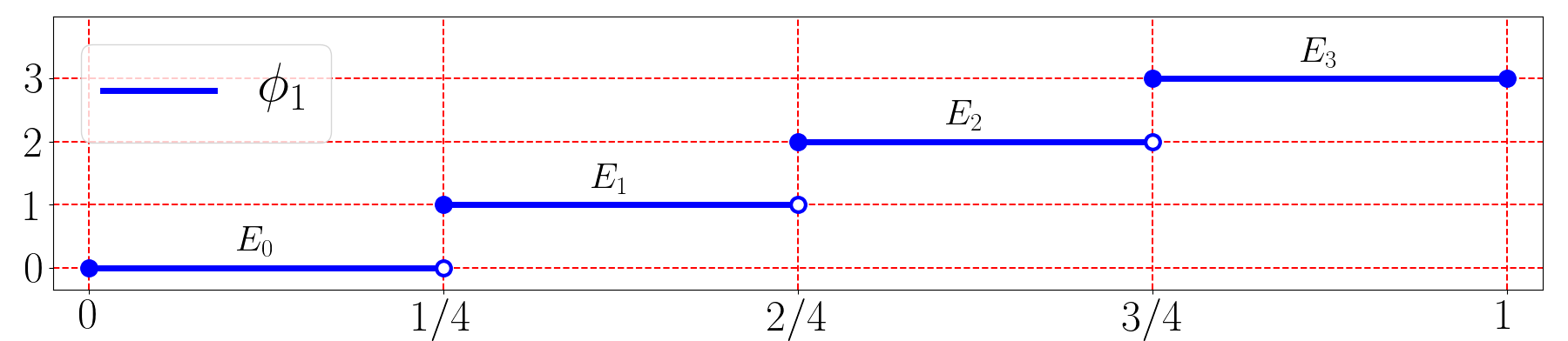
Figure 3: An illustration of $\phi_{1}$ on $[0,1]$ for the case $K=4$.

Define

$$\bm{\Phi}_{1}({\bm{x}})\coloneqq\big{(}\phi_{1}(x_{1}),\phi_{1}(x_{2}),\cdots,\phi_{1}(x_{d})\big{)},\quad\textnormal{for any ${\bm{x}}=(x_{1},x_{2},\cdots,x_{d})\in\mathbb{R}^{d}$.}$$

Clearly, we have, for ${\bm{x}}\in Q_{\bm{\beta}}$ and ${\bm{\beta}}\in\{0,1,\cdots,K-1\}^{d}$,

$$\bm{\Phi}_{1}({\bm{x}})=\big{(}\phi_{1}(x_{1}),\phi_{1}(x_{2}),\cdots,\phi_{1}(x_{d})\big{)}=(\beta_{1},\beta_{2},\cdots,\beta_{d})={\bm{\beta}}.$$

Step $3\colon$ Construct $\phi_{2}$ mapping ${\bm{\beta}}\in\{0,1,\cdots,K-1\}^{d}$ approximately to ${\widetilde{f}}({\bm{x}}_{\bm{\beta}})$.

Using the idea of $K$-ary representation, we define a linear function $\psi_{1}$ via

$$\psi_{1}({\bm{x}})\coloneqq 1+\sum_{j=1}^{d}x_{j}K^{j-1},\quad\textnormal{for any ${\bm{x}}=(x_{1},x_{2},\cdots,x_{d})\in\mathbb{R}^{d}$.}$$

Then $\psi_{1}$ is a bijection from $\{0,1,\cdots,K-1\}^{d}$ to $\{1,2,\cdots,K^{d}\}$.

Given any $i\in\{1,2,\cdots,K^{d}\}$, there exists a unique ${\bm{\beta}}\in\{0,1,\cdots,K-1\}^{d}$ such that $i=\psi_{1}({\bm{\beta}})$. Then define

$$\xi_{i}\coloneqq{\widetilde{f}}({\bm{x}}_{\bm{\beta}})\in[0,1],\quad\textnormal{for $i=\psi_{1}({\bm{\beta}})$ and ${\bm{\beta}}\in\{0,1,\cdots,K-1\}^{d}$,}$$

where ${\widetilde{f}}$ is the normalization of $f$ defined in Equation (6). It follows that there exists $\xi_{i,j}\in\{0,1\}$ for $j=1,2,\cdots,NL$ such that

$$|\xi_{i}-\textnormal{bin}\hskip 1.2pt0.\xi_{i,1}\xi_{i,2}\cdots,\xi_{i,NL}|\leq 2^{-NL},\quad\textnormal{for $i=1,2,\cdots,K^{d}$.}$$

By $K^{d}=(N^{L})^{d}=N^{dL}$ and Proposition 3.2, there exists a function $\psi_{2,j}$ implemented by a Floor-ReLU network with width $2N+2$ and depth $7dL-2$, for each $j=1,2,\cdots,NL$, such that

$$\psi_{2,j}(i)=\xi_{i,j},\quad\textnormal{for $i=1,2,\cdots,K^{d}$.}$$

Define

$$\psi_{2}\coloneqq\sum_{j=1}^{NL}2^{-j}\psi_{2,j}\quad\textnormal{and}\quad\phi_{2}\coloneqq\psi_{2}\circ\psi_{1}.$$

Then, for $i=\psi_{1}({\bm{\beta}})$ and ${\bm{\beta}}\in\{0,1,\cdots,K-1\}^{d}$, we have

$$\begin{split}|{\widetilde{f}}({\bm{x}}_{\bm{\beta}})-\phi_{2}({\bm{\beta}})|=|{\widetilde{f}}({\bm{x}}_{\bm{\beta}})-\psi_{2}(\psi_{1}({\bm{\beta}}))|&=|\xi_{i}-\psi_{2}(i)|=|\xi_{i}-\sum_{j=1}^{NL}2^{-j}\psi_{2,j}(i)|\\ &=|\xi_{i}-\textnormal{bin}\hskip 1.2pt0.\xi_{i,1}\xi_{i,2}\cdots\xi_{i,NL}|\leq 2^{-NL}.\end{split}$$ (7)

Step $4\colon$ Determine the final network to implement the desired function $\phi$.

Define ${\widetilde{\phi}}\coloneqq\phi_{2}\circ\bm{\Phi}_{1}$, i.e., for any ${\bm{x}}=(x_{1},x_{2},\cdots,x_{d})\in\mathbb{R}^{d}$,

$${\widetilde{\phi}}({\bm{x}})=\phi_{2}\circ\bm{\Phi}_{1}({\bm{x}})=\phi_{2}\big{(}\phi_{1}(x_{1}),\phi_{1}(x_{2}),\cdots,\phi_{1}(x_{d})\big{)}.$$

Note that $|{\bm{x}}-{\bm{x}}_{\bm{\beta}}|\leq\tfrac{\sqrt{d}}{K}$ for any ${\bm{x}}\in Q_{\bm{\beta}}$ and ${\bm{\beta}}\in\{0,1,\cdots,K-1\}^{d}$. Then we have, for any ${\bm{x}}\in Q_{\bm{\beta}}$ and ${\bm{\beta}}\in\{0,1,\cdots,K-1\}^{d}$,

$$\begin{split}|{\widetilde{f}}({\bm{x}})-{\widetilde{\phi}}({\bm{x}})|&\leq|{\widetilde{f}}({\bm{x}})-{\widetilde{f}}({\bm{x}}_{\bm{\beta}})|+|{\widetilde{f}}({\bm{x}}_{\bm{\beta}})-\widetilde{\phi}({\bm{x}})|\\ &\leq\omega_{\widetilde{f}}(\tfrac{\sqrt{d}}{K})+|{\widetilde{f}}({\bm{x}}_{\bm{\beta}})-\phi_{2}(\bm{\Phi}_{1}({\bm{x}}))|\\ &\leq\omega_{\widetilde{f}}(\tfrac{\sqrt{d}}{K})+|{\widetilde{f}}({\bm{x}}_{\bm{\beta}})-\phi_{2}({\bm{\beta}})|\leq\omega_{\widetilde{f}}(\tfrac{\sqrt{d}}{K})+2^{-NL},\end{split}$$

where the last inequality comes from Equation (7).

Note that ${\bm{x}}\in Q_{\bm{\beta}}$ and ${\bm{\beta}}\in\{0,1,\cdots,K-1\}^{d}$ are arbitrary. Since $[0,1]^{d}=\bigcup_{{\bm{\beta}}\in\{0,1,\cdots,K-1\}^{d}}Q_{\bm{\beta}}$, we have

$$|{\widetilde{f}}({\bm{x}})-{\widetilde{\phi}}({\bm{x}})|\leq\omega_{\widetilde{f}}(\tfrac{\sqrt{d}}{K})+2^{-NL},\quad\textnormal{for any ${\bm{x}}\in[0,1]^{d}$.}$$

Define

$$\phi\coloneqq 2\omega_{f}(\sqrt{d}){\widetilde{\phi}}+f({\bm{0}})-\omega_{f}(\sqrt{d}).$$

By $K=N^{L}$ and $\omega_{f}(r)=2\omega_{f}(\sqrt{d})\cdot\omega_{\widetilde{f}}(r)$ for any $r\geq 0$, we have, for any ${\bm{x}}\in[0,1]^{d}$,

$$\begin{split}|f({\bm{x}})-\phi({\bm{x}})|=2\omega_{f}(\sqrt{d})\big{|}{\widetilde{f}}({\bm{x}})-{\widetilde{\phi}}({\bm{x}})\big{|}&\leq 2\omega_{f}(\sqrt{d})\Big{(}\omega_{\widetilde{f}}(\tfrac{\sqrt{d}}{K})+2^{-NL}\Big{)}\\ &\leq\omega_{f}(\tfrac{\sqrt{d}}{K})+2\omega_{f}(\sqrt{d})2^{-NL}\\ &\leq\omega_{f}(\sqrt{d}\,N^{-L})+2\omega_{f}(\sqrt{d})2^{-NL}.\end{split}$$

It remains to determine the width and depth of the Floor-ReLU network implementing $\phi$. Clearly, $\phi_{2}$ can be implemented by the architecture in Figure 4.

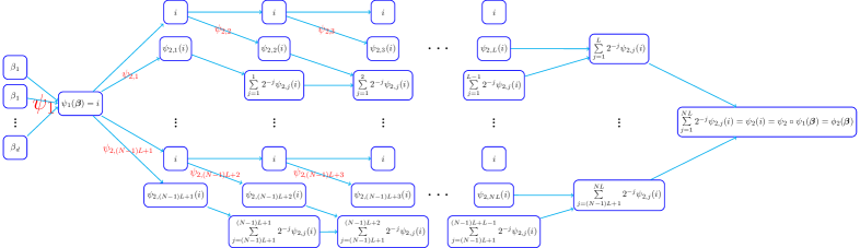
Figure 4: An illustration of the desired network architecture implementing $\phi_{2}=\psi_{2}\circ\psi_{1}$ for any input ${\bm{\beta}}\in\{0,1,\cdots,K-1\}^{d}$, where $i=\psi_{1}({\bm{\beta}})$.

As we can see from Figure 4, $\phi_{2}$ can be implemented by a Floor-ReLU network with width $N(2N+2+3)=2N^{2}+5N$ and depth $L(7dL-2+1)+2=L(7dL-1)+2$. With the network architecture implementing $\phi_{2}$ in hand, ${\widetilde{\phi}}$ can be implemented by the network architecture shown in Figure 5.

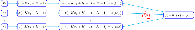
Figure 5: An illustration of the network architecture implementing ${\widetilde{\phi}}=\phi_{2}\circ{\bm{\Phi}}_{1}$.

Note that $\phi$ is defined via re-scaling and shifting ${\widetilde{\phi}}$. As shown in Figure 5, $\phi$ and ${\widetilde{\phi}}$ can be implemented by a Floor-ReLU network with width $\max\{d,\,2N^{2}+5N\}$ and depth $1+1+L(7dL-1)+2\leq 7dL^{2}+3$. So we finish the proof.

∎

4 Proof of Proposition 3.2

The proof of Proposition 3.2 mainly relies on the “bit extraction” technique. As we shall see later, our key idea is to apply the Floor activation function to make “bit extraction” more powerful to reduce network sizes. In particular, Floor-ReLU networks can extract much more bits than ReLU networks with the same network size.

Let us first establish a basic lemma to extract $1/N$ of the total bits of a binary number; the result is again stored in a binary number.

Lemma 4.1.

Given any $J,N\in\mathbb{N}^{+}$, there exists a function $\phi:\mathbb{R}^{2}\to\mathbb{R}$ that can be implemented by a Floor-ReLU network with width $2N$ and depth $4$ such that, for any $\theta_{j}\in\{0,1\}$, $j=1,\cdots,NJ$, we have

$$\phi(\textnormal{bin}\hskip 1.2pt0.\theta_{1}\cdots\theta_{NJ},\,n)=\textnormal{bin}\hskip 1.2pt0.\theta_{(n-1)J+1}\cdots\theta_{nJ},\quad\textnormal{for $n=1,2,\cdots,N$}.$$

Proof.

Given any $\theta_{j}\in\{0,1\}$ for $j=1,\cdots,NJ$, denote

$$s=\textnormal{bin}\hskip 1.2pt0.\theta_{1}\cdots\theta_{NJ}\quad\textnormal{and}\quad s_{n}=\textnormal{bin}\hskip 1.2pt0.\theta_{(n-1)J+1}\cdots\theta_{nJ},\quad\textnormal{for $n=1,2,\cdots,N$.}$$

Then our goal is to construct a function $\phi:\mathbb{R}^{2}\to\mathbb{R}$ computed by a Floor-ReLU network with the desired width and depth that satisfies

$$\phi(s,\,n)=s_{n},\quad\textnormal{for $n=1,2,\cdots,N$.}$$

Based on the properties of the binary representation, it is easy to check that

$$s_{n}=\lfloor 2^{nJ}s\rfloor\big{/}2^{{\color[rgb]{0,0,0}J}}-\lfloor 2^{(n-1)J}s\rfloor,\quad\textnormal{for $n=1,2,\cdots,N$}.$$ (8)

Even with the above formulas to generate $s_{1},s_{2},\cdots,s_{N}$, it is still technical to construct a network outputting $s_{n}$ for a given index $n\in\{1,2,\cdots,N\}$.

Set $\delta=2^{-{\color[rgb]{0,0,0}J}}$ and define $g$ (see Figure 6) as

$$g(x)\coloneqq\sigma\big{(}\sigma(x)-\sigma(\tfrac{x+\delta-1}{\delta})\big{)},\quad\textnormal{where $\sigma(x)=\max\{0,x\}$}.$$

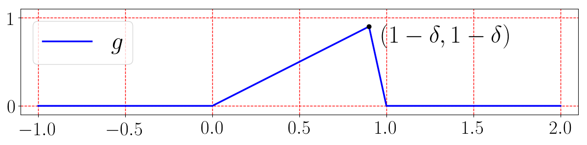
Figure 6: An illustration of $g(x)=\sigma\big{(}\sigma(x)-\sigma(\tfrac{x+\delta-1}{\delta})\big{)}$, where $\sigma(x)=\max\{0,x\}$ is the ReLU activation function.

Since $s_{n}\in[0,1-\delta]$ for $n=1,2,\cdots,N$, we have

$$s_{n}=\sum_{k=1}^{N}g(s_{k}+k-n),\quad\textnormal{for $n=1,2,\cdots,N$.}$$ (9)

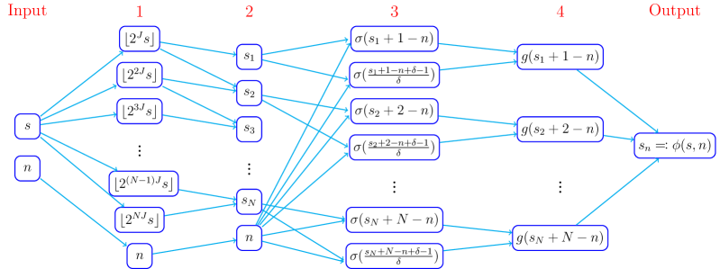
Figure 7: An illustration of the desired network architecture implementing $\phi$ based on Equation (8) and (9). We omit some ReLU ($\sigma$) activation functions when inputs are obviously non-negative. All parameters in this network are essentially determined by Equation (8) and (9), which are valid no matter what $\theta_{1},\cdots,\theta_{NJ}\in\{0,1\}$ are. Thus, the desired function $\phi$ implemented by this network is independent of $\theta_{1},\cdots,\theta_{NJ}\in\{0,1\}$.

As shown in Figure 7, the desired function $\phi$ can be computed by a Floor-ReLU network with width $2N$ and depth $4$. Moreover, it holds that

$$\phi(s,\,n)=s_{n},\quad\textnormal{for $n=1,2,\cdots,N$.}$$

So we finish the proof. ∎

The next lemma constructs a Floor-ReLU network that can extract any bit from a binary representation according to a specific index.

Lemma 4.2.

Given any $N,L\in\mathbb{N}^{+}$, there exists a function $\phi:\mathbb{R}^{2}\to\mathbb{R}$ implemented by a Floor-ReLU network with width $2N+2$ and depth $7L-3$ such that, for any $\theta_{m}\in\{0,1\}$, $m=1,2,\cdots,N^{L}$, we have

$$\phi(\textnormal{bin}\hskip 1.2pt0.\theta_{1}\theta_{2}\cdots\theta_{N^{L}},\,m)=\theta_{m},\quad\textnormal{for $m=1,2,\cdots,N^{L}$.}$$

Proof.

The proof is based on repeated applications of Lemma 4.1. Specifically, we inductively construct a sequence of functions $\phi_{1},\phi_{2},\cdots,\phi_{L}$ implemented by Floor-ReLU networks to satisfy the following two conditions for each $\ell\in\{1,2,\cdots,L\}$.

1. $\phi_{\ell}:\mathbb{R}^{2}\to\mathbb{R}$ can be implemented by a Floor-ReLU network with width $2N+2$ and depth $7\ell-3$.

2. For any $\theta_{m}\in\{0,1\}$, $m=1,2,\cdots,N^{\ell}$, we have

   $$\phi_{\ell}(\textnormal{bin}\hskip 1.2pt0.\theta_{1}\theta_{2}\cdots\theta_{N^{\ell}},\,m)=\textnormal{bin}\hskip 1.2pt0.\theta_{m},\quad\textnormal{for $m=1,2,\cdots,N^{\ell}$.}$$

Firstly, consider the case $\ell=1$. By Lemma 4.1 (set $J=1$ therein), there exists a function $\phi_{1}$ implemented by a Floor-ReLU network with width $2N\leq 2N+2$ and depth $4=7-3$ such that, for any $\theta_{m}\in\{0,1\}$, $m=1,2,\cdots,N$, we have

$$\phi_{1}(\textnormal{bin}\hskip 1.2pt0.\theta_{1}\theta_{2}\cdots\theta_{N},\,m)=\textnormal{bin}\hskip 1.2pt0.\theta_{m},\quad\textnormal{for $m=1,2,\cdots,N$.}$$

It follows that Condition (i) and (ii) hold for $\ell=1$.

Next, assume Condition (i) and (ii) hold for $\ell=k$. We would like to construct $\phi_{k+1}$ to make Condition (i) and (ii) true for $\ell=k+1$. By Lemma 4.1 (set $J=N^{k}$ therein), there exists a function $\psi$ implemented by a Floor-ReLU network with width $2N$ and depth $4$ such that, for any $\theta_{m}\in\{0,1\}$, $m=1,2,\cdots,N^{k{\color[rgb]{0,0,0}+1}}$, we have

$$\psi(\textnormal{bin}\hskip 1.2pt0.\theta_{1}\cdots\theta_{N^{k+1}},\,n)=\textnormal{bin}\hskip 1.2pt0.\theta_{(n-1)N^{k}+1}\cdots\theta_{(n-1)N^{k}+N^{k}},\quad\textnormal{for $n=1,2,\cdots,N$.}$$ (10)

By the hypothesis of induction, we have

• $\phi_{k}:\mathbb{R}^{2}\to\mathbb{R}$ can be implemented by a Floor-ReLU network with width $2N+2$ and depth $7k-3$.

• For any $\theta_{j}\in\{0,1\}$, $j=1,2,\cdots,N^{k}$, we have

  $$\phi_{k}(\textnormal{bin}\hskip 1.2pt0.\theta_{1}\theta_{2}\cdots\theta_{N^{k}},\,j)=\textnormal{bin}\hskip 1.2pt0.\theta_{j},\quad\textnormal{for $j=1,2,\cdots,N^{k}$.}$$ (11)

Given any $m\in\{1,2,\cdots,N^{k+1}\}$, there exist $n\in\{1,2,\cdots,N\}$ and $j\in\{1,2,\cdots,N^{k}\}$ such that $m=(n-1)N^{k}+j$, and such $n,j$ can be obtained by

$$n=\lfloor(m-1)/N^{k}\rfloor+1\quad\textnormal{and}\quad j=m-(n-1)N^{k}.$$ (12)

Then the desired architecture of the Floor-ReLU network implementing $\phi_{k+1}$ is shown in Figure 8.

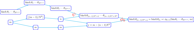
Figure 8: An illustration of the desired network architecture implementing $\phi_{k+1}$ based on (10), (11), and (12). We omit ReLU ($\sigma$) for neurons with non-negative inputs.

Note that $\psi$ can be computed by a Floor-ReLU network of width $2N$ and depth $4$. By Figure 8, we have

• $\phi_{k+1}:\mathbb{R}^{2}\to\mathbb{R}$ can be implemented by a Floor-ReLU network with width $2N+2$ and depth $2+4+1+(7k-3)=7(k+1)-3$, which implies Condition (i) for $\ell=k+1$.

• For any $\theta_{m}\in\{0,1\}$, $m=1,2,\cdots,N^{k+1}$, we have

  $$\phi_{k+1}(\textnormal{bin}\hskip 1.2pt0.\theta_{1}\theta_{2}\cdots\theta_{N^{k+1}},\,m)=\textnormal{bin}\hskip 1.2pt0.\theta_{m},\quad\textnormal{for $m=1,2,\cdots,N^{k+1}$.}$$

  That is, Condition (ii) holds for $\ell=k+1$.

So we finish the process of induction.

By the principle of induction, there exists a function $\phi_{L}:\mathbb{R}^{2}\to\mathbb{R}$ such that

• $\phi_{L}$ can be implemented by a Floor-ReLU network with width $2N+2$ and depth $7L-3$.

• For any $\theta_{m}\in\{0,1\}$, $m=1,2,\cdots,N^{L}$, we have

  $$\phi_{L}(\textnormal{bin}\hskip 1.2pt0.\theta_{1}\theta_{2}\cdots\theta_{{\color[rgb]{0,0,0}N}^{L}},\,m)=\textnormal{bin}\hskip 1.2pt0.\theta_{m},\quad\textnormal{for $m=1,2,\cdots,N^{L}$.}$$

Finally, define $\phi\coloneqq 2\phi_{L}$. Then $\phi$ can also be implemented by a Floor-ReLU network with width $2N+2$ and depth $7L-3$. Moreover, for any $\theta_{m}\in\{0,1\}$, $m=1,2,\cdots,N^{L}$, we have

$$\phi(\textnormal{bin}\hskip 1.2pt0.\theta_{1}\theta_{2}\cdots\theta_{N^{L}},\,m)=2\cdot\phi_{L}(\textnormal{bin}\hskip 1.2pt0.\theta_{1}\theta_{2}\cdots\theta_{N^{L}},\,m)=2\cdot\textnormal{bin}\hskip 1.2pt0.\theta_{m}=\theta_{m},$$

for $m=1,2,\cdots,N^{L}$. So we finish the proof. ∎

With Lemma 4.2 in hand, we are ready to prove Proposition 3.2.

Proof of Proposition 3.2.

By Lemma 4.2, there exists a function ${\widetilde{\phi}}:\mathbb{R}^{2}\to\mathbb{R}$ computed by a Floor-ReLU network with a fixed architecture with width $2N+2$ and depth $7L-3$ such that, for any $z_{m}\in\{0,1\}$, $m=1,2,\cdots,N^{L}$, we have

$${\widetilde{\phi}}(\textnormal{bin}\hskip 1.2pt0.z_{1}z_{2}\cdots z_{N^{L}},\,m)=z_{m},\quad\textnormal{for $m=1,2,\cdots,N^{L}$.}$$

Based on $\theta_{m}\in\{0,1\}$ for $m=1,2,\cdots,N^{L}$ given in Proposition 3.2, we define the final function $\phi$ as

$$\phi(x)\coloneqq{\widetilde{\phi}}\big{(}\sigma(x\cdot 0+\textnormal{bin}\hskip 1.2pt0.\theta_{1}\theta_{2}\cdots\theta_{N^{L}}),\sigma(x)\big{)},\quad\textnormal{where $\sigma(x)=\max\{0,x\}$.}$$

Clearly, $\phi$ can be implemented by a Floor-ReLU network with width $2N+2$ and depth $(7L-3)+1=7L-2$. Moreover, we have, for any $m\in\{1,2,\cdots,N^{L}\}$,

$$\phi(m)\coloneqq\widetilde{\phi}\big{(}\sigma(m\cdot 0+\textnormal{bin}\hskip 1.2pt0.\theta_{1}\theta_{2}\cdots\theta_{N^{L}}),\sigma(m)\big{)}=\widetilde{\phi}(\textnormal{bin}\hskip 1.2pt0.\theta_{1}\theta_{2}\cdots\theta_{N^{L}},m)=\theta_{m}.$$

So we finish the proof. ∎

We finally point out that only the properties of Floor on $[0,\infty)$ are used in our proof. Thus, the Floor can be replaced by the truncation function that can be easily computed by truncating the decimal part.

5 Conclusion

This paper has introduced a theoretical framework to show that deep network approximation can achieve root exponential convergence and avoid the curse of dimensionality for approximating functions as general as (Hölder) continuous functions. Given a Lipschitz continuous function $f$ on $[0,1]^{d}$, it was shown by construction that Floor-ReLU networks with width $\max\{d,\,5N+13\}$ and depth $64dL+3$ can achieve a uniform approximation error bounded by $3\lambda\sqrt{d}\,N^{-\sqrt{L}}$, where $\lambda$ is the Lipschitz constant of $f$. More generally for an arbitrary continuous function $f$ on $[0,1]^{d}$ with a modulus of continuity $\omega_{f}(\cdot)$, the approximation error is bounded by $\omega_{f}(\sqrt{d}\,N^{-\sqrt{L}})+2\omega_{f}(\sqrt{d}){N^{-\sqrt{L}}}$. The results in this paper provide a theoretical lower bound of the power of deep network approximation. Whether or not this bound is achievable in actual computation relies on advanced algorithm design as a separate line of research.

Acknowledgments. Z. Shen is supported by Tan Chin Tuan Centennial Professorship. H. Yang was partially supported by the US National Science Foundation under award DMS-1945029.

References

- Allen-Zhu et al., (2019) Allen-Zhu, Z., Li, Y., and Liang, Y. (2019). Learning and generalization in overparameterized neural networks, going beyond two layers. ArXiv, abs/1811.04918.
- Arnold, (1957) Arnold, V. I. (1957). On functions of three variables. Dokl. Akad. Nauk SSSR, pages 679–681.
- Arora et al., (2019) Arora, S., Du, S. S., Hu, W., Li, Z., and Wang, R. (2019). Fine-grained analysis of optimization and generalization for overparameterized two-layer neural networks. In ICML.
- Bao et al., (2019) Bao, C., Li, Q., Shen, Z., Tai, C., Wu, L., and Xiang, X. (2019). Approximation analysis of convolutional neural networks. Semantic Scholar e-Preprint, page Corpus ID: 204762668.
- Barron, (1993) Barron, A. R. (1993). Universal approximation bounds for superpositions of a sigmoidal function. IEEE Transactions on Information Theory, 39(3):930–945.
- Bartlett et al., (1998) Bartlett, P., Maiorov, V., and Meir, R. (1998). Almost linear VC-dimension bounds for piecewise polynomial networks. Neural Computation, 10:217–3.
- Bengio et al., (2013) Bengio, Y., Léonard, N., and Courville, A. (2013). Estimating or propagating gradients through stochastic neurons for conditional computation. arXiv e-prints, page arXiv:1308.3432.
- Berner et al., (2018) Berner, J., Grohs, P., and Jentzen, A. (2018). Analysis of the generalization error: Empirical risk minimization over deep artificial neural networks overcomes the curse of dimensionality in the numerical approximation of Black-Scholes partial differential equations. CoRR, abs/1809.03062.
- Bölcskei et al., (2019) Bölcskei, H., Grohs, P., Kutyniok, G., and Petersen, P. (2019). Optimal approximation with sparsely connected deep neural networks. SIAM Journal on Mathematics of Data Science, 1(1):8–45.
- Boo et al., (2020) Boo, Y., Shin, S., and Sung, W. (2020). Quantized neural networks: Characterization and holistic optimization. ArXiv, abs/2006.00530.
- Braun and Griebel, (2009) Braun, J. and Griebel, M. (2009). On a constructive proof of kolmogorov’s superposition theorem. Constructive Approximation, 30:653–675.
- Cao and Gu, (2019) Cao, Y. and Gu, Q. (2019). Generalization bounds of stochastic gradient descent for wide and deep neural networks. CoRR, abs/1905.13210.
- Carrillo et al., (2019) Carrillo, J. A. T., Jin, S., Li, L., and Zhu, Y. (2019). A consensus-based global optimization method for high dimensional machine learning problems. arXiv:1909.09249.
- Chen and Wu, (2019) Chen, L. and Wu, C. (2019). A note on the expressive power of deep rectified linear unit networks in high-dimensional spaces. Mathematical Methods in the Applied Sciences, 42(9):3400–3404.
- (15) Chen, M., Jiang, H., Liao, W., and Zhao, T. (2019a). Efficient approximation of deep ReLU networks for functions on low dimensional manifolds. In Wallach, H., Larochelle, H., Beygelzimer, A., d'Alché-Buc, F., Fox, E., and Garnett, R., editors, Advances in Neural Information Processing Systems 32, pages 8174–8184. Curran Associates, Inc.
- (16) Chen, Z., Cao, Y., Zou, D., and Gu, Q. (2019b). How much over-parameterization is sufficient to learn deep ReLU networks? CoRR, arXiv:1911.12360.
- Chui et al., (2018) Chui, C. K., Lin, S.-B., and Zhou, D.-X. (2018). Construction of neural networks for realization of localized deep learning. Frontiers in Applied Mathematics and Statistics, 4:14.
- Cybenko, (1989) Cybenko, G. (1989). Approximation by superpositions of a sigmoidal function. MCSS, 2:303–314.
- Devore, (1989) Devore, R. A. (1989). Optimal nonlinear approximation. Manuskripta Math, pages 469–478.
- E et al., (2019) E, W., Ma, C., and Wu, L. (2019). A priori estimates of the population risk for two-layer neural networks. Communications in Mathematical Sciences, 17(5):1407 – 1425.
- E and Wang, (2018) E, W. and Wang, Q. (2018). Exponential convergence of the deep neural network approximation for analytic functions. CoRR, abs/1807.00297.
- E and Wojtowytsch, (2020) E, W. and Wojtowytsch, S. (2020). Representation formulas and pointwise properties for barron functions.
- Gribonval et al., (2019) Gribonval, R., Kutyniok, G., Nielsen, M., and Voigtlaender, F. (2019). Approximation spaces of deep neural networks. arXiv e-prints, page arXiv:1905.01208.
- Gühring et al., (2019) Gühring, I., Kutyniok, G., and Petersen, P. (2019). Error bounds for approximations with deep ReLU neural networks in norms. arXiv e-prints, page arXiv:1902.07896.
- Guliyev and Ismailov, (2018) Guliyev, N. J. and Ismailov, V. E. (2018). Approximation capability of two hidden layer feedforward neural networks with fixed weights. Neurocomputing, 316:262 – 269.
- Harvey et al., (2017) Harvey, N., Liaw, C., and Mehrabian, A. (2017). Nearly-tight VC-dimension bounds for piecewise linear neural networks. In Kale, S. and Shamir, O., editors, Proceedings of the 2017 Conference on Learning Theory, volume 65 of Proceedings of Machine Learning Research, pages 1064–1068, Amsterdam, Netherlands. PMLR.
- Holland, (1992) Holland, J. H. (1992). Genetic algorithms. Scientific American, 267(1):66–73.
- Hornik et al., (1989) Hornik, K., Stinchcombe, M., and White, H. (1989). Multilayer feedforward networks are universal approximators. Neural Networks, 2(5):359 – 366.
- Hubara et al., (2017) Hubara, I., Courbariaux, M., Soudry, D., El-Yaniv, R., and Bengio, Y. (2017). Quantized neural networks: Training neural networks with low precision weights and activations. J. Mach. Learn. Res., 18(1):6869–6898.
- Igelnik and Parikh, (2003) Igelnik, B. and Parikh, N. (2003). Kolmogorov’s spline network. IEEE Transactions on Neural Networks, 14(4):725–733.
- Jacot et al., (2018) Jacot, A., Gabriel, F., and Hongler, C. (2018). Neural tangent kernel: Convergence and generalization in neural networks. CoRR, abs/1806.07572.
- Ji and Telgarsky, (2020) Ji, Z. and Telgarsky, M. (2020). Polylogarithmic width suffices for gradient descent to achieve arbitrarily small test error with shallow ReLU networks. ArXiv, abs/1909.12292.
- Kennedy and Eberhart, (1995) Kennedy, J. and Eberhart, R. (1995). Particle swarm optimization. In Proceedings of ICNN’95 - International Conference on Neural Networks, volume 4, pages 1942–1948 vol.4.
- Kirkpatrick et al., (1983) Kirkpatrick, S., Gelatt, C. D., and Vecchi, M. P. (1983). Optimization by simulated annealing. Science, 220(4598):671–680.
- Kolmogorov, (1956) Kolmogorov, A. N. (1956). On the representation of continuous functions of several variables by superposition of continuous functions of a smaller number of variables. Dokl. Akad. Nauk SSSR, pages 179–182.
- Kolmogorov, (1957) Kolmogorov, A. N. (1957). On the representation of continuous functions of several variables by superposition of continuous functions of one variable and addition. Dokl. Akad. Nauk SSSR, pages 953–956.
- Kůrková, (1992) Kůrková, V. (1992). Kolmogorov’s theorem and multilayer neural networks. Neural Networks, 5(3):501 – 506.
- Li et al., (2019) Li, Q., Lin, T., and Shen, Z. (2019). Deep learning via dynamical systems: An approximation perspective. arXiv e-prints, page arXiv:1912.10382.
- Liang and Srikant, (2016) Liang, S. and Srikant, R. (2016). Why deep neural networks? CoRR, abs/1610.04161.
- Lin et al., (2019) Lin, Y., Lei, M., and Niu, L. (2019). Optimization strategies in quantized neural networks: A review. In 2019 International Conference on Data Mining Workshops (ICDMW), pages 385–390.
- Lu et al., (2020) Lu, J., Shen, Z., Yang, H., and Zhang, S. (2020). Deep network approximation for smooth functions. arXiv e-prints, page arXiv:2001.03040.
- Luo and Yang, (2020) Luo, T. and Yang, H. (2020). Two-layer neural networks for partial differential equations: Optimization and generalization theory. ArXiv, abs/2006.15733.
- Maiorov and Pinkus, (1999) Maiorov, V. and Pinkus, A. (1999). Lower bounds for approximation by MLP neural networks. Neurocomputing, 25(1):81 – 91.
- Montanelli and Du, (2019) Montanelli, H. and Du, Q. (2019). New error bounds for deep ReLU networks using sparse grids. SIAM Journal on Mathematics of Data Science, 1(1):78–92.
- Montanelli and Yang, (2020) Montanelli, H. and Yang, H. (2020). Error bounds for deep ReLU networks using the Kolmogorov-Arnold superposition theorem. Neural Networks, 129:1 – 6.
- Montanelli et al., (2020) Montanelli, H., Yang, H., and Du, Q. (2020). Deep ReLU networks overcome the curse of dimensionality for bandlimited functions. Journal of Computational Mathematics.
- Nakada and Imaizumi, (2019) Nakada, R. and Imaizumi, M. (2019). Adaptive approximation and estimation of deep neural network with intrinsic dimensionality. arXiv:1907.02177.
- Nelder and Mead, (1965) Nelder, J. and Mead, R. (1965). A simplex method for function minimization. Comput. J., 7:308–313.
- Opschoor et al., (2019) Opschoor, J. A. A., Schwab, C., and Zech, J. (2019). Exponential ReLU DNN expression of holomorphic maps in high dimension. Technical Report 2019-35, Seminar for Applied Mathematics, ETH Zürich, Switzerland. https://math.ethz.ch/sam/research/reports.html?id=839.
- Petersen and Voigtlaender, (2018) Petersen, P. and Voigtlaender, F. (2018). Optimal approximation of piecewise smooth functions using deep ReLU neural networks. Neural Networks, 108:296 – 330.
- Pinnau et al., (2017) Pinnau, R., Totzeck, C., Tse, O., and Martin, S. (2017). A consensus-based model for global optimization and its mean-field limit. Mathematical Models and Methods in Applied Sciences, 27(01):183–204.
- Poggio et al., (2017) Poggio, T., Mhaskar, H. N., Rosasco, L., Miranda, B., and Liao, Q. (2017). Why and when can deep—but not shallow—networks avoid the curse of dimensionality: A review. International Journal of Automation and Computing, 14:503–519.
- (53) Shen, Z., Yang, H., and Zhang, S. (2019a). Nonlinear approximation via compositions. Neural Networks, 119:74 – 84.
- (54) Shen, Z., Yang, H., and Zhang, S. (2019b). Deep network approximation characterized by number of neurons. arXiv e-prints, page arXiv:1906.05497.
- Suzuki, (2019) Suzuki, T. (2019). Adaptivity of deep ReLU network for learning in Besov and mixed smooth Besov spaces: optimal rate and curse of dimensionality. In International Conference on Learning Representations.
- Wang et al., (2018) Wang, P., Hu, Q., Zhang, Y., Zhang, C., Liu, Y., and Cheng, J. (2018). Two-step quantization for low-bit neural networks. In 2018 IEEE/CVF Conference on Computer Vision and Pattern Recognition, pages 4376–4384.
- Yang and Wang, (2020) Yang, Y. and Wang, Y. (2020). Approximation in shift-invariant spaces with deep ReLU neural networks. arXiv e-prints, page arXiv:2005.11949.
- Yarotsky, (2017) Yarotsky, D. (2017). Error bounds for approximations with deep ReLU networks. Neural Networks, 94:103 – 114.
- Yarotsky, (2018) Yarotsky, D. (2018). Optimal approximation of continuous functions by very deep ReLU networks. In Bubeck, S., Perchet, V., and Rigollet, P., editors, Proceedings of the 31st Conference On Learning Theory, volume 75 of Proceedings of Machine Learning Research, pages 639–649. PMLR.
- Yarotsky and Zhevnerchuk, (2019) Yarotsky, D. and Zhevnerchuk, A. (2019). The phase diagram of approximation rates for deep neural networks. arXiv e-prints, page arXiv:1906.09477.
- Yin et al., (2019) Yin, P., Lyu, J., Zhang, S., Osher, S., Qi, Y., and Xin, J. (2019). Understanding straight-through estimator in training activation quantized neural nets. ArXiv, abs/1903.05662.
- Zhou, (2020) Zhou, D.-X. (2020). Universality of deep convolutional neural networks. Applied and Computational Harmonic Analysis, 48(2):787 – 794.